1. INTRODUCTION
The study of relativistic dynamics of a charged particle in electromagnetic fields is of prime importance in high intensity laser-matter interaction. Integrability and chaos are the key to predicting conditions for stochastic heating that can take place when very nonlinear regimes are reached. Recently, particle-in-cell (PIC) code simulations results published by Tajima et al. (Reference Tajima, Kishimoto and Masaki2001) and theoretical results obtained by Mulser et al. (Reference Mulser, Kanapathipillai and Hoffmann2005) and Ziaja et al. (Reference Ziaja, Weckert and Moller2007) have shown that the irradiation of very high intensity lasers on clustered matter leads to a very efficient heating of electrons. Tajima et al. (Reference Tajima, Kishimoto and Masaki2001) and Kanapathipillai (Reference Kanapathipillai2006) have shown that chaos seems to be the origin of the strong laser coupling with clusters. It was confirmed in PIC code simulations, in the case of two counter-propagating laser pulses, that stochastic heating can lead to efficient electron acceleration (Sheng et al., Reference Sheng, Mima, Zhang and Meyer-Ter-Vehn2004, Reference Sheng, Mima, Sentoku, Jovanovic, Taguchi, Zhang and Meyer-Ter-Vehn2002; Bourdier et al., Reference Bourdier, Patin and Lefebvre2007, Reference Bourdier, Patin and Lefebvre2005a; Patin, Reference Patin2006; Patin et al., Reference Patin, Lefebvre, Bourdier and D'humieres2006, Reference Patin, Bourdier and Lefebvre2005a, Reference Patin, Bourdier and Lefebvre2005b). In this field, many issues need to be studied. Those that we will address below are mainly the stability of the electron motion in the fields of one electromagnetic wave propagating in vacuum or in plasma, and the conditions for stochastic heating to take place. At very high intensities, the motion of a charged particle in a wave is highly nonlinear. The situations when the motion is integrable are exceptional. The solutions corresponding to these situations deserve to be studied as they are strong as predicted by the Kolmogorov-Arnold-Moser (KAM) theorem (Lichtenberg & Liebermann, Reference Lichtenberg and Liebermann1983; Arnold, Reference Arnold1988; Rasband, Reference Rasband1983; Ott, Reference Ott1993; Tabor, Reference Tabor1989; Walker & Ford, Reference Walker and Ford1969). In some situations, they are necessary to predict resonances, build-up perturbation calculations, and predict conditions to trigger stochastic heating.
The dynamic of a charged particle in a linearly or almost linearly polarized traveling high intensity wave is studied when it propagates in a nonmagnetized medium first. The problem is shown to be Liouville integrable when the wave propagates in vacuum. In this situation, the equation of Hamilton-Jacobi is also solved showing the integrability of the system again and also giving resonance conditions when a perturbing wave is taken into account (Bourdier et al., Reference Bourdier, Patin and Lefebvre2007, Reference Bourdier, Patin and Lefebvre2005a, Reference Bourdier and Patin2005b; Patin, Reference Patin2006; Patin et al., Reference Patin, Lefebvre, Bourdier and D'humieres2006, Reference Patin, Bourdier and Lefebvre2005a, Reference Patin, Bourdier and Lefebvre2005b; Rax, Reference Rax1992). When the wave propagates in plasma, the plasma response is partly taken into account by introducing an index, n, in the equations. Then, the problem is still integrable. The effect of the full plasma response is studied next by considering plasma wave equations. In their paper, Kaw et al. (Reference Kaw, Sen and Valeo1983) shown an apparent absence of chaos for the system that was thus promoted to a good position in the list of systems waiting for the proof of their integrability. An exhaustive numerical study of the system allowed us to witness chaotic trajectories, showing that the system is not integrable. The stochastic behavior of trajectories was first seen in the laboratory frame by performing Poincaré maps and confirmed by calculating a nonzero Lyapunov exponent (Bourdier, Reference Bourdier2009). The same kind of numerical work was achieved in a special Lorentz frame where the variables that describe the waves are space independent (Winkles & Eldridge, Reference Winkles and Eldridge1972). The numerical work happens to be easier in this frame as, at least some chaotic trajectories, fill larger volumes in phase space.
Then, the wave is assumed to propagate along a constant homogeneous magnetic field in vacuum or in plasma. In a first part, the electromagnetic wave is assumed to propagate in vacuum. It is shown that the synchronous solution discussed by Roberts and Buchsbaum (Reference Roberts and Buchsbaum1964) in the case of a circularly polarized wave still exists when the wave is linearly polarized. One of the constants of motion is present in the resonance condition (Davydovski, Reference Davydovski1963); it implies that when the charged particle is initially resonant, it gains energy indefinitely. Two constants that are canonically conjugate are found. This property is used to reduce the initially three degrees of freedom problem to two degrees of freedom problem. The system that was shown to be Liouville integrable (Lichtenberg & Liebermann, Reference Lichtenberg and Liebermann1983; Arnold, Reference Arnold1988; Rasband, Reference Rasband1983; Ott, Reference Ott1993; Tabor, Reference Tabor1989; Bouquet & Bourdier, Reference Bouquet and Bourdier1998; Bourdier et al., Reference Bourdier, Patin and Lefebvre2007, Reference Bourdier, Patin and Lefebvre2005a, Reference Bourdier and Patin2005b) is integrated in this paper. Then, in order to study the plasma response in the case of a very high intensity wave propagating in low-density plasma, it is assumed that the wave remains linearly polarized. Performing a Lorentz transformation eliminates the space variable corresponding to the direction of propagation of the wave (Winkles & Eldridge, Reference Winkles and Eldridge1972). Just like above, two canonically conjugate constants are used to reduce the initially three degrees of freedom problem to two degrees of freedom problem. Thus, Poincaré maps are performed. Lyapunov exponents are also calculated to confirm the chaotic nature of some trajectories (Lichtenberg & Liebermann, Reference Lichtenberg and Liebermann1983; Ott, Reference Ott1993; Tabor, Reference Tabor1989; Bourdier & Michel-Lours, Reference Bourdier and Michel-Lours1994). Chaos appears when a secondary resonance and a primary resonance overlap (Bourdier et al., Reference Bourdier, Patin and Lefebvre2007, Reference Bourdier, Patin and Lefebvre2005a, Reference Bourdier and Patin2005b; Patin, Reference Patin2006; Patin et al., Reference Patin, Lefebvre, Bourdier and D'humieres2006, Reference Patin, Bourdier and Lefebvre2005b; Kwon & Lee, Reference Kwon and Lee1999; Van Der Weele et al., Reference Van Der Weele, Capel, Valkering and Post1998). Consequently, the system is not integrable and chaos appears as soon as the plasma response is taken into account.
The interaction of low density plasma with a high intensity plane wave perturbed by another plane wave is studied next. The stability of a single particle interacting with two waves is studied first. The solution of Hamilton-Jacobi equation, in the case of a single particle interacting with one wave, is used to identify resonances. The effect of the different parameters is shortly described by using the Chirikov (Reference Chirikov1979) criterion. Stochastic heating is seen by computing single particle energies. At last, considering plasma, PIC code simulations results obtained with the code CALDER (Lefebvre et al., Reference Lefebvre, Cochet, Fritzler, Malka, Aleonard, Chemin, Darbon, Disdier, Faure, Fedotoff, Landoas, Malka, Meot, Morel, Rabec Le Gloahec, Rouyer, Rubbelynck, Tikhonchuk, Wrobel, Audebert and Rousseaux2003) are presented in order to validate the theoretical model for experimentally relevant parameters. The stochastic acceleration that is shown in this part can explain how the Wakefield acceleration can be boosted by using a counter-propagating wave (Davoine et al., 2008). For example, in the work published by Mikhailov et al. (Reference Mikhailov, Nikitina, Sklizkov, Starodub and Zhurovich2008), the fact that an efficient electron heating takes place when a counter-propagating wave is reflected from the critical density can be partially explained with this model.
Finally, let us point out that a lot of experimental work is being achieved in order to use stochastic acceleration and also, for instance, on laser interaction with clusters, where stochastic heating is predicted to play an important role (Faenov et al., Reference Faenov, Magunov, Pikuz, Skobelev, Giulietti, Betti, Galimberti, Gamucci, Giulietti, Gizzi, Labate, Levato, Tomassini, Marques, Bourgeois, Dobosz Dufrenoy, Ceccotti, Monot, Reau, Popescu, D'oliveira, Martin, Fukuda, Boldarev, Gasilov and Gasilov2008).
2. DYNAMICS OF A CHARGED PARTICLE IN A LINEARLY POLARIZED ELECTROMAGNETIC TRAVELING WAVE PROPAGATING IN A NON-MAGNETIZED MEDIUM
2.1. The Wave Propagates in Vacuum
2.1.1. Hamiltonian Formulation of the Problem: Integrability of the System
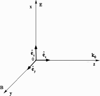
Let us consider a charged particle in an electromagnetic plane wave propagating along the z direction (Fig. 1). The following four-potential is chosen for the wave

where E0, ω0, k0 are constants and  is the unit vector along the x-axis.
Frame of reference.

When time is treated as a parameter entirely distinct from the spatial coordinates, the relativistic Hamiltonian of a charged particle in an electromagnetic wave is given by:  , where −e, m, and P are, respectively, the particle's charge, its rest mass, and its canonical momentum. In the present situation, it reads

where the Pi (i = x, y, z) are the canonical momentum components. This system has three degrees of freedom. The following dimensionless variables and parameter are introduced next
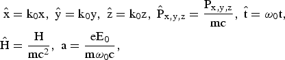
and the canonical transformation,  , given by the type-2 generating function

is performed (Lichtenberg & Liebermann, Reference Lichtenberg and Liebermann1983; Arnold, Reference Arnold1988; Rasband, Reference Rasband1983; Ott, Reference Ott1993; Tabor, Reference Tabor1989; Bourdier & Gond, Reference Bourdier and Gond2000; Bouquet & Bourdier, Reference Bouquet and Bourdier1998). Let us recall that when performing a canonical transformation  defined by a type-2 generating function
 , where
 and
 are the new coordinates, and pi and qi are the old ones, the canonical transformation is given by (Lichtenberg & Liebermann, Reference Lichtenberg and Liebermann1983; Arnold, Reference Arnold1988; Rasband, Reference Rasband1983; Ott, Reference Ott1993; Tabor, Reference Tabor1989)
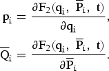
Consequently, the generating function defined by Eq. (4) yields the canonical spatial transformation

This canonical transformation keeps  unchanged and yields a new normalized Hamiltonian given by
 , that is to say,

This Hamiltonian is autonomous as it is a function of the three momenta  ,
 ,
 , and ς which are space coordinate (we have called the value of the Hamiltonian Ĉ),
 ,
 , and
 are three constants of motion, which are independent and in involution and, as a consequence, the system is completely integrable (Lichtenberg & Liebermann, Reference Lichtenberg and Liebermann1983; Arnold, Reference Arnold1988; Rasband, Reference Rasband1983; Ott, Reference Ott1993; Tabor, Reference Tabor1989).
2.1.2. Integration of the Hamilton-Jacobi Equation
When using the proper time of the particle to parameterize the motion in the extended phase space, the Hamiltonian of the charged particle in the wave reads (Jackson, Reference Jackson1975)

where γ is the Lorentz factor. Within the scope of this Hamiltonian formulation one has H = 0 (Jackson, Reference Jackson1975). This zero-value Hamiltonian is satisfactory in the sense that it allows us to derive the right equations of motion. Then, the dimensionless variables and parameter defined by equations (3) are used again, a normalized proper time:  and a normalized vector potential: a = eA/mc are also introduced. The normalized Hamiltonian reads

It is assumed that the electron motion is restricted to the plane of polarization of the wave (the y degree of freedom is assumed not to be excited). We look for a set of actions (P⊥, P//, E) and angles (θ, φ, ϕ), instead of the configuration (r, t), and momentum, (P, −γ) in the  phase space. In other words, we seek a canonical transformation
 , such that the new momenta are constants of motion. It will be shown further that P⊥ and P// represent the drift motion of the charged particle and E its average energy normalized to mc2. To do so, we look for a generating function,
 such that
 ,
 , γ = ∂F2/∂t that is a solution of the Hamilton-Jacobi equation (Arnold, Reference Arnold1988; Rasband, Reference Rasband1983; Ott, Reference Ott1993; Tabor, Reference Tabor1989; Goldstein, Reference Goldstein1980; Landau & Lifshitz, Reference Landau and Lifshitz1975)


Following Landau and Lifshitz (Reference Landau and Lifshitz1975), it is assumed that F2 has the following form

where the quantities α1, α2, and α3 are chosen to be three independent constants of integration in order to select three new constant momenta. Letting  , Eq. (11) becomes

Solving this equation leads to
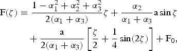
where F0 is a constant with respect to ζ, which is assumed to vanish as only partial derivatives of F(ζ) are considered. Letting
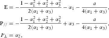
as: α1 + α3 = P// − E, the following expression is found for F2 (Landau & Lifshitz, Reference Landau and Lifshitz1975; Rax, Reference Rax1992)
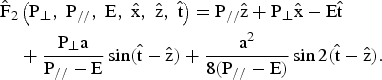
The old configuration variables expressed in terms of the new ones are given by (Rax, Reference Rax1992)
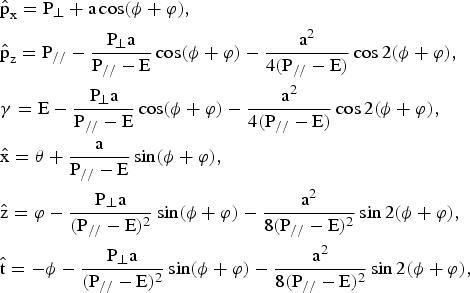
where  and
 are the components of the normalized momentum of the charged particle
 . It is straightforward to check that,
 ,
 , E = 〈γ〉 ( <> stands for averaging over the oscillations), and Ĉ = E − P//. All the former constants of motion are found again. P// and P⊥ describe the uniform motion of translation that is obtained by averaging out the oscillatory part of the motion. The new Hamiltonian in terms of the action variables reads (Rax, Reference Rax1992)

where M2 = 1 + a 2/2. As  (Jackson, Reference Jackson1975), the energy momentum dispersion relation is given by

The solution of Hamilton equations is

Finding the solution of Hamilton-Jacobi equation is another way to prove that the problem is integrable. This solution is also very useful to predict resonances when a perturbing mode is considered (Bourdier et al., Reference Bourdier, Patin and Lefebvre2007, Reference Bourdier, Patin and Lefebvre2005a, Reference Bourdier and Patin2005b; Patin, Reference Patin2006; Patin et al., Reference Patin, Lefebvre, Bourdier and D'humieres2006, Reference Patin, Bourdier and Lefebvre2005b; Rax, Reference Rax1992).
2.2. The Wave Propagates in Plasma
2.2.1. The Plasma Index of Refraction is Introduced to Describe a Part of the Plasma Influence
A part of the influence of the plasma is taken into account first by simply introducing the index of the medium in the equation of propagation of waves in vacuum. It is shown in Section 3, in the case of a plane wave propagating along a constant homogeneous magnetic field, that including an index of refraction in this very simple way is enough to make the system non-integrable (Bourdier et al., Reference Bourdier, Patin and Lefebvre2007, Reference Bourdier, Patin and Lefebvre2005a, Reference Bourdier and Patin2005b; Patin, Reference Patin2006). The wave vector potential is supposed to be given by Eq. (1). The dimensionless variables and parameters previously defined are used again. The normalized equations can be derived through the normalized Hamiltonian: Ĥ = nγ = nH/mc2, where n is the index of refraction of the plasma. This Hamiltonian reads

 ,
 , and
 are still three constants of motion. As they are independent and in involution, the system is still integrable.
2.2.2. The Full plasma Response is Taken into Account Through Plasma Wave Equations
Following Akhiezer and Polovin (Reference Akhiezer and Polovin1956), the propagation of a relativistically strong wave in cold relativistic electron plasma is described with Maxwell and Lorentz equations. All the variables entering into these equations are assumed not to be functions of space and time separately, but only of the combination i · r − Vt, where i is a constant unit vector parallel to the direction of propagation of the wave, and V is a constant. Then, the equations describing nonlinear traveling waves propagating in the absence of the external magnetic field are as follows:
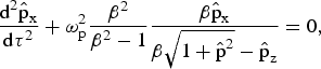
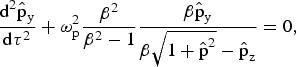

where  is the normalized hydrodynamic momentum, τ = t − i · r/V, β = V/c, and ωp is the plasma frequency. Letting θ = ωp(β2 − 1)−1/2 τ, these equations read
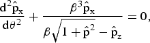
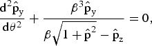

When considering that the electron motion is in the x-z plane  , we let
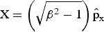 and
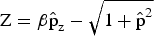 , then, Eq. (23) become
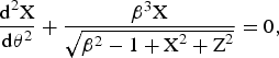

Eqs. (24a and 24b) can obviously be derived from the Hamiltonian

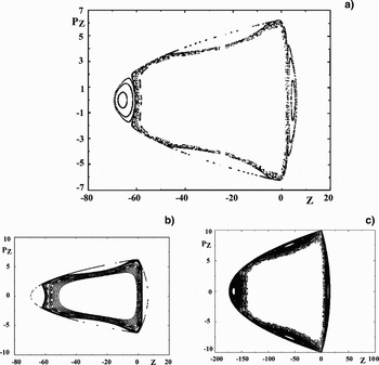
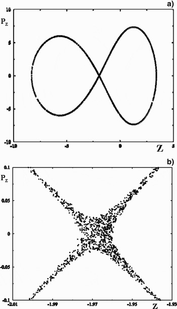
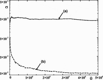
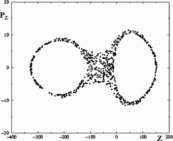
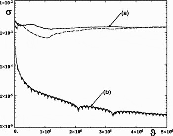
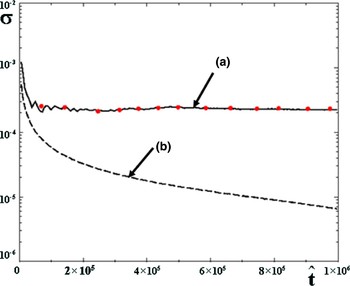
where PX = dX/dθ and PZ = dZ/dθ. Then, the coupled stationary wave problem can be treated as a two-degree-of-freedom conservative problem. Consequently, Poincaré maps can be performed. Since the Hamiltonian is symmetric in X, the X-oscillator can be used as a clock and PZversus Z can be plotted each time X = 0 and PX > 0. The problem looks integrable; most of the Poincaré maps obtained are regular (Fig. 2) and most of theLyapunov exponents calculated go to zero (Kaw et al., Reference Kaw, Sen and Valeo1983; Bourdier, Reference Bourdier2009). Still, chaos was found considering one trajectory for which chaos takes place in a very small volume in phase space (Fig. 3). Chaos appears when enlarging a lot the place where it takes place; therefore, it was difficult to know if it were numerical chaos or real chaos (Fig. 3b). Consequently, the Lyapunov exponent of this trajectory was carefully calculated by using Benettin's method (Lichtenberg & Liebermann, Reference Lichtenberg and Liebermann1983; Tabor, Reference Tabor1989; Bourdier & Michel-Lours, Reference Bourdier and Michel-Lours1994). To do this, two very close trajectories are considered, the very small distance between them being initially d0. A sequence dn corresponding to these trajectories is calculated numerically. For every fixed time Δt, or for every fixed distance ratio dn/d0 ≈ 2, dn is renormalized to d0. The two ways to renormalize are used and compared, Figure 4 shows the good agreement obtained for the nonzero the Lyapunov exponent calculated when using the two ways. It shows that it is real chaos and that, consequently, the problem is not integrable.
Poincaré surface of section plots in the laboratory frame: PZversus Z (X = 0, Px > 0). H = 20, β = 1.2. (a, b): Several trajectories are considered. H = 50, β = 1.2. (c): Several trajectories are considered.

Poincaré surface of section plots in the laboratory frame: PZ versus Z (X = 0, Px > 0). H = 248.824, β = 3.24. (a) One trajectory is considered. (b) Enlargement of part of the stochastic orbit.

Lyapunov exponents: (a) Lyapunov exponents calculated for the same initial conditions as those of the trajectory shown in Figures 3a, 3b. The two renormalization techniques are performed, they give almost the same results. (b) Lyapunov exponent corresponding to a regular trajectory.

Introducing ϑ = β3θ, n = 1/β, Eqs. (24a and 24b) become
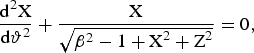

Letting,  and
 , dropping the tildes for the sake of simplicity, Eqs. (26a and 26b) can be derived from the following Hamiltonian

Then, the problem is under the form studied by Grammaticos et al. (Reference Grammaticos, Ramani and Yoshida1987). In their paper, they claim that this system is not integrable. Following their paper very high energies are considered (X2 + Z2 ≫ β2 − 1), then Eqs. (26a and 26b) read
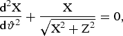
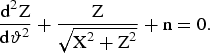
These equations can be derived from the Hamiltonian

with

This system corresponds to the limit of infinite energy. Hamiltonian (29a and 29b) is Hamiltonian (27) when β2 = 1. It was shown that if Hamiltonian (27) were meromorphic, then system (27) would not be integrable when system (29a and 29b) is not (Juillard Tosel, Reference Juillard Tosel2000, Reference Juillard Tosel1999). It is not clear a priori whether this property can be applied to our problem as Hamiltonian (27) is not meromorphic. Still, the right system is described by this Hamiltonian (Eqs. 29a and 29b) plus a small quantity that depends on β (in the limit of high energies). Then, if system (29a and 29b) is not integrable, system (27) is probably not integrable for an arbitrary value of this parameter; in other words, the exact system that corresponds to an arbitrary energy is likely to be nonintegrable. Poincaré maps have been performed within this high energy limit system. They show that the system defined by Hamiltonian (29a and 29b) exhibit chaotic trajectories in some conditions (Fig. 5).
Poincaré surface of section plots in the laboratory frame: PZ versus Z (X = 0, Px > 0). H = 248.824, β = 3.24. One trajectory is considered.

The Lyapunov exponent for the trajectory corresponding to Figure 5 is calculated by using Benettin's method (Eqs 6, 10, 21). The two ways to renormalize are used and compared; Figure 6 shows the good agreement obtained for the nonzero Lyapunov exponent when using the two renormalization techniques. The fact that the system (29a and 29b) is not integrable backs up the previous assertion that says that the exact system is not integrable.
Lyapunov exponents: (a) Lyapunov exponents calculated for the same initial conditions as those of the trajectory shown in Figure 5. The two renormalizations are performed; they give almost the same results. (b) Lyapunov exponent corresponding to a regular trajectory.

Then, another frame is considered to look for chaotic trajectories. This is to make absolutely sure that this very important result concerning the integrability of the problem is right. Following Winkles and Eldridge (Reference Winkles and Eldridge1972) and Romeiras (Reference Romeiras1989), a new frame (L*) that moves uniformly along the z-axis with velocity U relative to the laboratory frame is introduced. The Lorentz transformation of the four-momentum is given by (Jackson, Reference Jackson1975; Landau & Lifshitz, Reference Landau and Lifshitz1975)

where Γ = (1 − U2/c2)−1/2 and E = γmc2 are the energy of the charged particle. In the extended phase space, where time is treated on a common basis with other coordinates, a fully covariant Hamiltonian formulation of the problem can be constructed. In this space, the Lorentz transformation defined above is identical to the canonical transformation generated by the following type-2 generating function

As a consequence, if the hydrodynamic motion is not integrable in the frame (L*), it is also not integrable in the laboratory frame. The phase of the wave that is an invariant takes, in the moving frame, the following form (Jackson, Reference Jackson1975; Landau & Lifshitz, Reference Landau and Lifshitz1975)

When the phase velocity of the wave is greater than the speed of light, there exists one special frame (L*) in which the phase does not depend on the variable z′. This frame has the following drift velocity: U/c = k0c/ω0 = n (Winkles & Eldridge, Reference Winkles and Eldridge1972). Still considering that the electron motion is in the x–z plane  , the wave Eqs. (23a, 23b, 23c) read
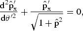
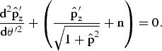
where θ′ = ω′pt′ (ω′p is the plasma frequency in (L*)). Introducing  ,
 , P′X′ = dX′/dθ′ and P′Z′ = dZ′/dθ′, dropping the primes for convenience, Eqs. (33a and 33b) can be derived from the following Hamiltonian

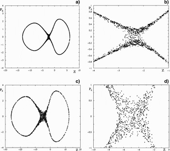
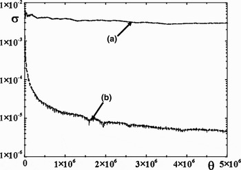
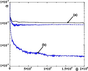
Then, the problem is under the form studied by Grammaticos et al. (Reference Grammaticos, Ramani and Yoshida1987) again. Poincaré maps are performed, PZversus Z is plotted each time X = 0 and PX > 0. Figures 7 show chaotic trajectories. In one case, chaos is confirmed by calculating a nonzero Lyapunov exponent (Fig. 8). In short, it has been shown numerically that in both the laboratory frame and in (L*), the problem is not integrable.
Poincaré surface of section plots in (L*): PZversus Z (X = 0, Px > 0). H = 10, n = 0.3. (a) One trajectory is considered. (b) Enlargement of part of the stochastic orbit H = 20, n = 0.3. (c) One trajectory is considered. (d) Enlargement of part of the stochastic orbit

Lyapunov exponents: (a) Lyapunov exponents calculated for the same initial conditions as those of the trajectory shown in Figures 7c, 7d. The two renormalizations techniques are performed and give almost the same results. (b) Lyapunov exponent corresponding to a regular trajectory.

3. DYNAMICS OF A CHARGED PARTICLE IN A LINEARLY POLARIZED ELECTROMAGNETIC TRAVELING WAVE PROPAGATING ALONG A CONSTANT HOMOGENEOUS MAGNETIC FIELD
3.1. The Wave Propagates in Vacuum
3.1.1. Hamiltonian and Symmetries of the System
Let us consider a charged particle in an electromagnetic plane wave propagating along the z direction (the wave vector k0 is parallel to the z direction). The constant magnetic field B0 is supposed to be along the z-axis. The traveling wave is assumed to be linearly polarized. It has a propagation vector k0 parallel to B0.
The following vector potential is chosen for the electromagnetic field

The scalar potential is assumed to vanish. The relativistic Hamiltonian for the motion is
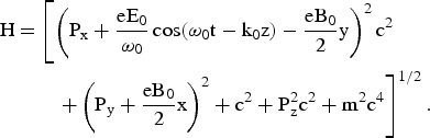
This is a time-dependent system with three degrees of freedom. It can be easily checked that

is a constant of motion for this system. Combining the equations of Hamilton allows us to easily find two other constants of motion

These two constants are such that
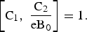
The three constants just found are not in involution and, at this stage, one cannot conclude that the problem is integrable.
The normalized equations of motion are obtained by introducing the normalized variables and parameters defined by Eq. (3) and Ω0 = eB0/mω0. The following three normalized constants are also introduced Ĉ = C/mc2, Ĉ1 = C1/mc, and Ĉ2 = C2/mc.
3.1.2. Reduction to a Two Degrees of Freedom Problem Integration of the System
The canonical transformation  :
 , is performed first (Bourdier & Gond, Reference Bourdier and Gond2000; Bouquet & Bourdier, Reference Bouquet and Bourdier1998). The Hamiltonian expressed in terms of the new variables is
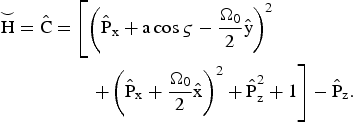
In this new system, ς plays the part of a space coordinate. The new Hamiltonian is a constant as it does not depend explicitly on time.
The fact that the two constants Ĉ1 and Ĉ1/Ω0 are canonically-conjugate is used to reduce the system. To do so, a canonical transformation:  , which is the product of two canonical transformations is performed (Bourdier & Gond, Reference Bourdier and Gond2000; Bourdier et al., Reference Bourdier, Valentini and Valat1996; Michel-Lours et al., Reference Michel-Lours, Bourdier and Buzzi1992). The first canonical transformation:
 is defined by the following type-2 generating functions:


In these variables C1 and C2 become:  and
 . The second transformation:
 , is generated by


The resulting transformation, which is the product of the two transformations, is given by
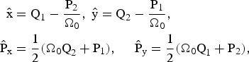
With these new variables, one has: Q2 = Ĉ1/Ω0 and P2 = Ĉ2. The degree of freedom associated to the conjugate variables (Q2, P2) is eliminated. Thus, the initially three degrees of freedom system is reduced to a two degree of freedom system. In terms of the new conjugate variables: (Q1, P1) and  , the new Hamiltonian is

The equations of Hamilton are
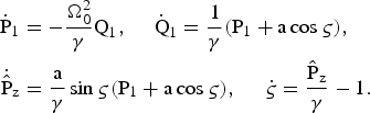
The equation of Hamilton for ς, can be put in the form 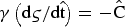 . As a consequence, indicating differentiation with respect to ς by a prime in this paragraph, we can write
 , which implies that
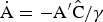 . Thus, the equations of Hamilton (Eqs. (45)) become
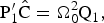



Differentiating a second time the second equation leads to the following equation of motion for Q1
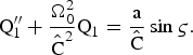
The following equation for P1 is obtained in the same way
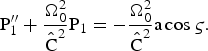
These two equations (47a and 47b) are the equations of two driven oscillators. One has a resonance when  . This resonance condition contains a first integral of the system, this implies that when the particle is initially resonant it remains resonant forever (Roberts & Buchsbaum, Reference Roberts and Buchsbaum1964; Davydovski, Reference Davydovski1963; Bourdier & Gond, Reference Bourdier and Gond2001, Reference Bourdier and Gond2000). These equations can be easily solved analytically whether the resonance condition is satisfied or not. Then Eq. (46c) is used to determine Pz and γ is derived through Eq. (46d). The Liouville integrability of this problem can also be shown easily (Bourdier et al., Reference Bourdier, Patin and Lefebvre2007, Reference Bourdier, Patin and Lefebvre2005a, Reference Bourdier and Patin2005b; Patin, Reference Patin2006).
3.2. The Wave Propagates in Plasma
3.2.1. Existence of an Almost Linearly Polarized Solution at Very High Intensities
Here again, all the variables entering into these equations describing nonlinear traveling waves are assumed not to be functions of space and time separately, but only of the combination i · r – Vt. Then, the equations describing waves propagating along a constant homogeneous external magnetic field are the following (Akhiezer & Polovin, Reference Akhiezer and Polovin1956)
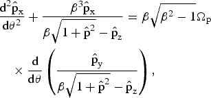
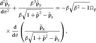

where Ωp = ωc/ωp with ωc = eB0/m.
Let us consider transverse solutions (solutions such that:  ). Eq. (48c) implies that
 is a constant. The transverse solution has to be a solution of the following set of two equations
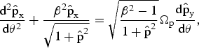
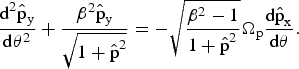
One can look for transverse monochromatic plane waves (fixing ω0) which are solution of this set of equation. The following left-handed circularly polarized wave
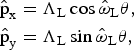
is a solution of Eqs. (49a and 49b) if
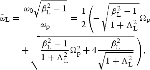
where ω0 is the time-frequency fixed by the light source.
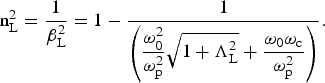
The index of refraction for this mode is given by
The following transverse right-handed circularly polarized wave
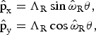
is a solution when

This implies that
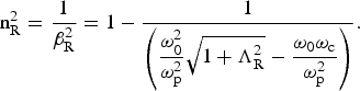
Equations (51b, 53b) allows us to find again the well-known indexes of refraction for the left-handed wave and the right-handed wave when ΛL,R → 0 (Swanson, Reference Swanson1989).
As two different phase velocities correspond to these two solutions, one cannot conclude that their sum represents a slow rotating wave solution of Eqs. (49a and 49b). Thus, we now look for almost linearly solutions which are plane waves that is to say solutions corresponding to one given phase velocity (β is fixed). When introducing the complex quantity 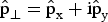 and assuming for simplicity that the index of refraction of the medium is close to unity, Eqs. (49) are equivalent to the following complex equation

where 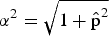 and
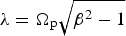 . The solution is given by
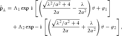
where Λ1, Λ2, φ1, and φ2 are real constants which depend on the initial conditions. This leads to


This solution contains two frequencies. Taking into account the fact that 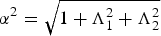 ,
 and
 read
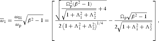
and
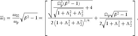
Let us consider a frame of reference rotating slowly clockwise with an angular velocity—Ω. In this new frame, the solution in the plane perpendicular to the propagation direction is the solution given by Eq. (55) multiplied by expiΩθ. The solution reads


Assuming that Λ1 = Λ2 and φ1 = φ2 = 0,  equals zero when Ω = (ω2 − ω1)/2, then, the solution of by Eq. (55) becomes


where  and
 . This solution represents a rotating wave in the plane perpendicular to its direction of propagation with the following angular velocity
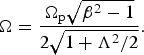
This rotation is not the classical Faraday rotation as the field rotates for a given value of z. The rotation rate versus τ is
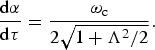
It decreases when the intensity of the wave increases. As a consequence, almost linearly polarized plane waves can propagate when very high intensities are considered. This legitimates the fact that the Faraday rotation is ignored in the next paragraph.
3.2.2. Only the Plasma Index of Refraction is Introduced to Describe the Plasma Influence: The Wave is Assumed to Remain Linearly Polarized when Propagating in Plasma
In this part, the influence of plasma is taken into account. The wave is assumed to remain linearly polarized. The wave vector potential is supposed to be given by Eq. (35). The dimensionless variables and parameters previously defined are used again. The normalized Hamiltonian of the system,  , where n is the index of refraction of the plasma, reads

The Hamilton equations allow us to readily find two constants of motion
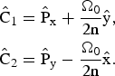
It can be noted that the two constants Ĉ1 and nĈ2/Ω0 are canonically conjugate.  is still a constant of motion. These three constants of motion are not in involution and one cannot conclude that the problem is integrable.
Then, the frame (L*), previously defined is considered again. In (L*), the vector potential is assumed to be

The equations of motion are generated by the following Hamiltonian
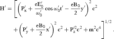
Let us now introduce the following dimensionless variables and parameters
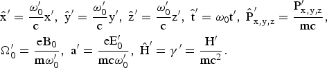
The following normalized Hamiltonian

leads to the normalized equations of motion.
Dropping the primes for convenience, it can be shown very easily that this system has three constants of motion

The first two constants (Ĉ1 and Ĉ2/Ω0) are canonically conjugate.
Let us reduce the system in order to perform Poincaré maps. To do so, let us choose the two constants Ĉ1 and Ĉ2 as new momentum and coordinate conjugate. The canonical transformation defined by Eqs. (43) is performed. The new Hamiltonian is

This is a time-dependent system with only two degrees of freedom. As  is an obvious first integral, one can evacuate the conjugate variable Ẑ and say, even if it is not academic, that we have a time-dependent system with one degree of freedom.
Let us perform now the following canonical transformation

generated by

The Hamiltonian in terms of the new variables is

This is still a time-dependent system with only two degrees of freedom.  is still a constant of motion. The equations of Hamilton read
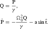
This set of equations is similar to the one found by Kwon and Lee (Reference Kwon and Lee1999) when describing the motion of a particle in a constant and homogeneous magnetic field and an oscillating electric field of arbitrary polarization. These equations of motion are solved numerically. We have assumed that  in every case. Chaos is evidenced first by performing Poincaré maps. The plane P − Q with
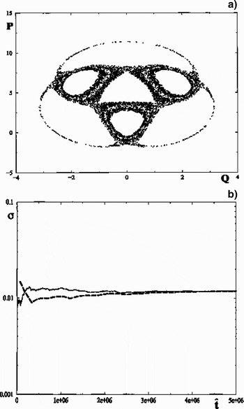
 (mod2π) is chosen to be the Poincaré surface of section. Figure 9a shows Poincaré maps for only one trajectory. The chaotic nature of this trajectory is confirmed by calculating a nonzero Lyapunov exponent by using Benettin's method (Lichtenberg & Liebermann, Reference Lichtenberg and Liebermann1983; Tabor, Reference Tabor1989; Bourdier & Michel-Lours, Reference Bourdier and Michel-Lours1994). The two ways to renormalize are used and compared, Figure 9b shows the good agreement obtained for the Lyapunov exponents when using the two renormalization techniques. The fact that we have chaotic trajectories shows that the system is not integrable.
a = 4.03, Ω0 = 2. (a) Surface of section plots for one trajectory. (b) Lyapunov exponent calculated with the same trajectory, the two renormalization methods are compared.

When going back to the laboratory frame, the equations of Hamilton must be derived through Hamiltonian (62). In order to reduce the system, two canonical transformations defined by the following type-2 generating functions  and
 are performed. The new Hamiltonian reads

The equations of Hamilton are
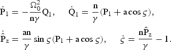
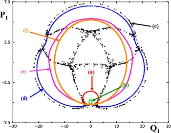
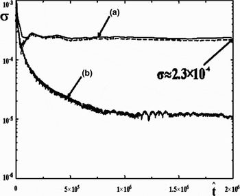
When the index of refraction is very close to unity, chaotic trajectories were evidenced by performing Poincaré maps and calculating Lyapunov exponents (Figs. 10, 11). Figure 10 shows Poincaré maps obtained with the same initial conditions in the integrable case when n = 1 and in nonintegrable cases. The trajectory of the charged particle changes dramatically when n is close to unity. Figure 11 shows the Lyapunov exponents calculated through Eqs. (75) for the chaotic trajectory (n = 0.99) and the integrable one (n = 1).
(Color online) Surface of section plots. Ω0 = 0.282, a = 4.03. (a) n = 1. (b) n = 0.999. (c) n = 0.99. (d) n = 0.988. (e) n = 0.95. (f): n = 0.8.

Lyapunov exponents for two trajectories. Ω0 = 0.282, a = 4.03. (a) n = 0.99 (the two ways to renormalize are used). (b) n = 1.

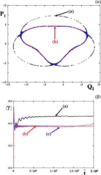
Considering that the index of refraction of the plasma and the magnetic field are fixed, when varied in the range (3.88 to 3.9), the trajectory becomes chaotic and suddenly visits a larger phase space and reaches a higher average energy (Fig. 12).
(Color online) Ω0 = 0.282, n = 0.99. (a) a = 3.9. (b) a = 3.88. (c) a = 3.86. (α): Surface of section plots for two trajectories. (β): Average Lorentz factor of the particle versus time.

A nonzero Lyapunov exponent is also calculated in the laboratory frame in terms of the  variables confirming the nonintegrability of the problem (Fig. 13).
(Color online) Lyapunov exponent calculated for one trajectory in the laboratory frame in terms of the 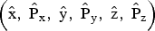 variables. Ω0 = 0.282, a = 4.03. (a) n = 0.99, the two renormalization methods are used, the red circles are obtained by renormalizing dn to d0 every fixed distance ratio d/d0. (b) n = 0.2.

In order to estimate the effect of the Faraday rotation very crudely, a slow varying phase is introduced in the expression of the electromagnetic field. The following Hamiltonian is considered
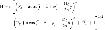
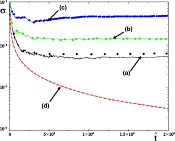
The phase φ is assumed to be given by φ = εz where ε is a small quantity. Different Lyapunov exponents are calculated for different values of ε and are compared to the Lyapunov exponent of a regular trajectory (n = 0.2). For one trajectory, assuming that ε is in the range [0–10−3], the Lyapunov exponent increases when ε increases; chaos increases as the Faraday rotation becomes more significant (Fig. 14).
(Color online) Lyapunov exponent calculated for some initial conditions. Ω0 = 0.282, a = 2.85. The two renormalization methods are used; the circles are obtained by renormalizing dn to d0 every fixed distance ratio d/d0. (a) n = 0.99, ε = 0. (b) n = 0.99, ε = 10−4, (c) n = 0.99, ε = 10−3, (d) n = 0.2, ε = 0.

3.2.3. The Full Plasma Response Is Taken Into Account through Plasma Wave Equations
Letting  and
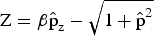 , Eqs. (48) become
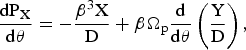
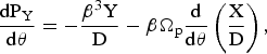
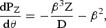
where  , PX = dX/dθ, PY = dY/dθ, and PZ = dZ/dθ. When Ωp = 0, Eqs. (77) can obviously be derived from the following Hamiltonian

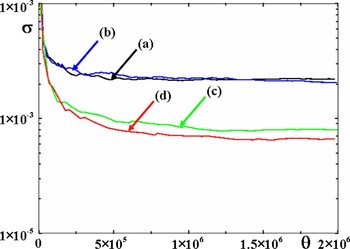
Positive Lyapunov exponents were also calculated for initial conditions very close to those for which chaos is seen when only n is considered to take into account the plasma response (Fig. 15). The fact that the entire plasma response is taken into consideration spreads out the initial conditions for chaos to take place (Fig. 16).
(Color online) Lyapunov exponents. (a) Positive Lyapunov exponents calculated by using the two ways to renormalize. H0 = 248.824 [calculated with Eq. (80)], Ωp = 0.01 and β = 3.24. (b) Lyapunov exponent corresponding to a regular trajectory.

(Color online) Positive Lyapunov exponents calculated when Ωp = 1.999. Each time the distance ratio dn/d0 ≈ 2, the distance dn is renormalized to d0. (a) H 0 = 0.442, β = 1.0101. (b) H0 = 0.449, β = 1.012. (c) H0 = 0.814, β = 1.1. (d) H0 = 1.664, β = 1.25.

4. DYNAMICS OF A CHARGED PARTICLE IN TWO LINEARLY POLARIZED TRAVELING ELECTROMAGNETIC WAVES PROPAGATING IN A NONMAGNETIZED VACUUM
4.1. Compton Resonances
Let us consider a charged particle in a high intensity electromagnetic plane wave propagating along the z direction (the wave vector k0 is parallel to the z direction) perturbed by a low intensity wave. The high intensity mode 4-potential is given by Eq. (1).
In this theoretical part, the perturbing wave is assumed to have its electric fields in the polarization plane of the high intensity wave. Considering that the polarization plane of the high intensity mode is the plane of reference, this situation is called the P–polarization case.
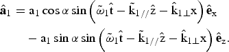
The Hamiltonian of an electron in the two waves is given by:

and is approximated by:

with
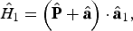
A straightforward but cumbersome calculation shows that (Patin, 2006; Bourdier et al., 2005a, 2005b; Rax, 1992)

where N is a negative integer. When the phase of the sine is stationary, the perturbation calculation fails to converge because of the occurrence of a small denominator. On the basis of the solution of Hamilton-Jacobi in the case of one wave, this stationary condition gives the Compton resonance condition

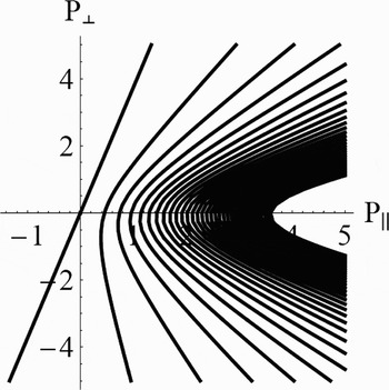
Figure 17 displays P⊥ versus P// restricted to the energy surface Eq. (19).
Compton resonances. α = 5π/6, a = 1,  .

4.2. Influence of the Different Parameters. Chirikov Criterion
Let us show how to choose the different parameters in order to optimize the stochastic heating. Trajectories are chaotic when their initial conditions stand in the overlapping region of two or several resonances.
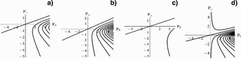
Figure 18 display the Compton resonances (P⊥versus P//) for different situations. They show their influence on the resonance pattern. Only the first resonances are shown in these figures. The resonance lines become closer for growing values of α and  while higher values of a have the opposite effect. The resonance lines become symmetric with respect to the P // axis when α grows. Figures 17 and 18 seem to show that chaos will be optimum when α is close to π.
Compton resonances for different values of the parameters. (a) α = π/6, a = 1,  , (b) α = π/4, a = 1,
 , (c) α = π/6, a = 4,
 , (d) α = π/6, a = 1,


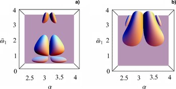
At this level, one cannot come to a conclusion as these behaviors must be compared to the one of the resonance widths. Only the ratio of the sum of the half-widths of two resonances over the distance separating them allows a conclusion. When this ration is higher than unity, the two resonances overlap, the Chirikov threshold criterion is fulfilled and trajectories which have their initial conditions in overlapping region are chaotic. Chaos will be widely spread in phase space when the Chirikov criterion is satisfied for many resonances. Then stochastic heating can take place. Two resonances only, were considered and conditions for the Chirikov threshold to be reached were explored. To do so, the ratio  where ΔP⊥,//,N + ΔP⊥,//,N′ is the sum of the half-widths of the resonances and dN,N′ is the distance which separates them was calculated (Bourdier et al., 2007, 2005a, 2005b; Patin, 2006; Patin et al., 2006, 2005b). Figure 19 show that the Chirikov criterion is better satisfied when α in is close to π, in the range (5π/6, 7π/6). The best choice is for resonances N = −1 and N = −2, when
 is in the range (1, 2). The criterion is also satisfied when
 and α ∈ [9π/10, 11π/10]. With respect to the resonances N = −2 and N = −3, a higher value of
 must be considered, one must have
 .
(Color online) Chirikov criterion: RN,N′ as a function of different parameters when P⊥ = 0. a = 1, a1 = 0.1, (a) Resonances N = −1 and N = −2, (b) N = −2 and N = −3.

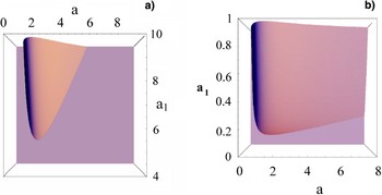
Figure 20 show the influence on the Chirikov criterion of a and a1. When α = π/6 (Fig. 20a), the Chirikov threshold can be reached only outside the scope of this model (a 1 < a). It can be reached, for instance, for a = 4 and a 1 = 0.4 when α = 5π/6 (Fig. 20b).
(Color online) Chirikov criterion: RN,N′ in function of electric field amplitudes when P⊥ = 0. Resonances N = −1 and N = −2. (a)  , α = π/6, (b)
 , α = 5π/6.

In summary, the Chirikov criterion will be satisfied when α is close to π and almost only the resonances N = −1 and N = −2 can overlap when P⊥ does not equal zero. Extended chaos can take place in a banana-like surface in the (P⊥, P//) phase space.
4.3. Numerical Evidence of Stochastic Heating by Considering a Single Particle or Plasma
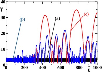
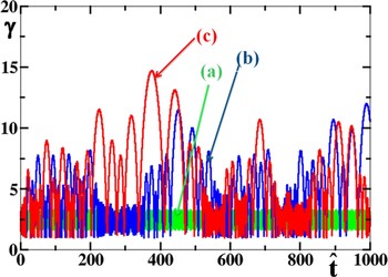
First, stochastic acceleration was seen by considering a single particle. The normalized energy of the particle was calculated with a fourth order Runge-Kutta, Figure 21 shows its evolution considering one and two waves. Figure 21a shows the Lorentz factor when the total intensity is in one wave. Figures 21b and 21c show the same when the total intensity is in two waves. Figures 21b and 21c were obtained for two different integration step sizes (h), the difference between the two curves is a signature of chaos. Thus, Figure 21 displays heating associated to chaos.
(Color online) Energy of one particle versus time. P-polarization.  , α = 5π/6,
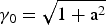 , (γ0 is the initial Lorentz factor). (a) one wave case, a = 4.0112, a1 = 0. (b) two waves case, a = 4, a1 = 0.3, h = 10−3, (c) two waves case a = 4, a1 = 0.3, h = 10−4

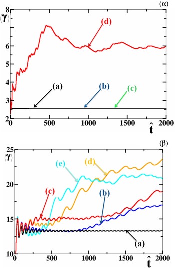
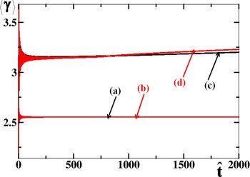
As it has been shown above that stochastic heating is close to maximum when α is close to π, consequently, the case of two counter-propagating waves was specially considered. Moreover, this 1D configuration allowed us to perform rapid PIC code simulations. Figure 22 shows the existence of a threshold for stochastic heating. For one given value of a, there is a threshold value for a 1 so that significant stochastic heating may take place. For two different initial conditions (the initial Lorentz factor is 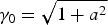 and γ0 = 1) when a = 3, substantial stochastic heating takes place when a1 is greater than about 0.1 (Figs. 22 and 23).
(Color online) Energy of one particle in two waves versus time. P-polarization. a = 3,  , α = π,
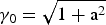 . (a) a1 = 0.1. (b) a1 = 0.25. (c) a1 = 0.3.

(Color online) Average energy of one particle versus time. P-polarization.  , α = π. (α):
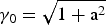 . (a) One wave case: a = 3.0016, a1 = 0. (b) Two waves case: a = 3, a1 = 0.1. (c) Two waves case: a = 3, a1 = 0.2. (d) Two waves case: a = 3, a 1 = 0.3. (β): γ0 = 1, a = 3. (a) a1 = 0. (b) a1 = 0.08. (c) a1 = 0.1, (d): a1 = 0.2, (e): a1 = 0.3

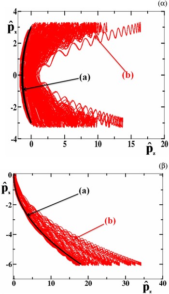
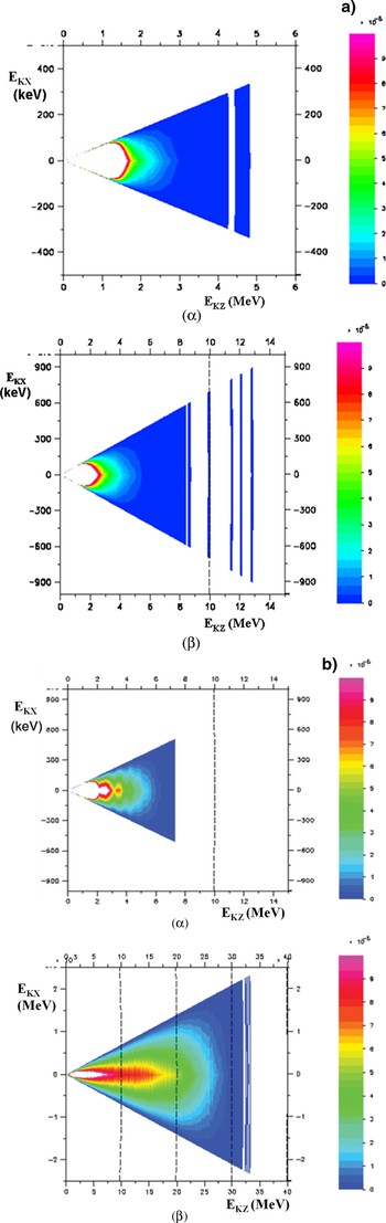
Figure 24 show the phase space visited by a single particle when considering two different initial conditions. They show that when the low intensity counter-propagating wave is taken into account, particles undergo a stochastic acceleration in the direction of propagation of the high intensity wave. Low density plasma kinetic 1Dz3Dv (one spatial coordinate and three velocity coordinates) PIC simulations were achieved with the code CALDER partly in order to confirm the acceleration mechanism predicted by the single particle approach. A trapezoidal electronic density profile plasma with a 10 c/ω0 slope and a homogeneous slab which occupies a region of 100 µm step with a density, Ne = 10−2Nc (Nc is the critical density for a 1 µm laser wavelength), is considered. The plasma is assumed to have an initial temperature of 1 keV, ions are supposed to be a continuous neutralizing background. A quadratic interpolation shape factor ensuring optimal energy conservation (ΔE/E < 10−3) given the ratio Δx/λD ≈ 0.25 (Δx is the spatial step size of each mesh and λD the Debye length) is used. A very good sampling of the phase space is performed using two hundred particles per mesh. The laser pulses are assumed to be two semi-infinite steps with the same 1 µm wavelength; the peak intensity is reached after some time: t L. A smooth intensity profile was considered here: t L = 50 τ0, where τ0 is the time of a laser cycle. Figures 25 exhibit electron phase space when considering respectively one semi-infinite laser wave with a = 3 or two colliding waves with a = 3 and a 1 = 0.3, that is to say, when the maximum intensities are I = 1.23 1019 W/cm2 and I = 1.23 1017 W/cm2, respectively, for the high and low intensity wave. Figure 25b shows higher densities than Figure 25a along the E k,z axis thus confirming acceleration along the propagation direction of the high intensity wave.
(Color online) Phase space. P-polarization.  , α = π, (α):
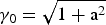 . (a) One wave case: a = 3.015, a1 = 0. (b): Two waves case: a = 3, a1 = 0.3. (β): γ0 = 1. (a) One wave case: a = 3.0016, a1 = 0. (b) Two waves case: a = 3, a1 = 0.1.

(Color online) (a) Energy spectrum in the case of one wave at two different times. a = 3, a1 = 0,  ,α = π. tL = 50 τ0. (α): τ = 756 ω0−1. (β): τ = 2916ω0−1. t. (b) Energy spectrum at two different times in the case of two waves. P-polarization. a = 3, a1 = 0.3,
 , α = π. tL = 50 τ0. (α): τ = 756 ω0−1. (β): τ = 2916 ω0−1.

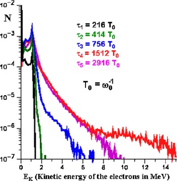
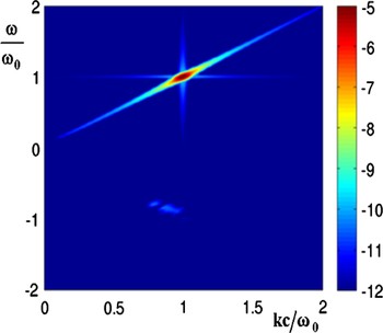
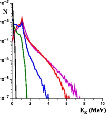
Figure 26 shows the electron energy distribution at five different times, when considering a single semi-infinite laser pulse with a = 3. In this case, the peak intensity of the laser pulse is assumed to be reached after t L = 9.77 τ0. The first time τ1 = 216 T0 (T 0 = ω0−1) is when the wave has covered about 25% of the plasma, the second time τ2 = 414 T 0 is when the wave has run through about the half of the plasma, at τ3 = 756 T 0 the wave has reached the plasma boundary. The two last times τ4 = 1512 T 0 and τ5 = 2916 T 0 correspond to situations when the plasma really interacts with two plane waves. The hot electron tail reaches a maximum energy well after the wave has crossed the entire plasma at times close to τ4 = 1512 T 0. The maximum energy reached by the distribution function drops with times as evidenced by the pink curve at τ4 = 2916 T 0. In the physical situation considered here some electrons are trapped in the wakefield until the wave comes to the plasma-vacuum boundary, this phenomenon is responsible for the hot electron tail observed in Figure 26 at 1512 T 0. The steep laser pulse gradient creates a wakefield which is responsible for some electron trapping and acceleration. The wakefield acceleration is almost ruled out when considering a smoother laser pulse gradient or lower electron densities. It is also ruled out at lower intensities. The intensity of Raman backscattering remains about four orders of magnitude below the one of the high intensity wave (Fig. 27); consequently, it plays no role in this hot tail generation.
(Color online) Electron energy distribution from 1D PIC simulations at different times. P-polarization. The plasma slab is with a thickness of L = 100 µm and a density at Ne = 0.01 Nc. tL = 9.77 τ0. A semi-infinite laser pulse is incident with a peak amplitude a = 3.

(Color online) Color map in log scale of the space – time Fourier transform of the transverse electromagnetic field. P polarization. The plasma slab is with a thickness of L = 100 µm and a density at Ne = 0.01 Nc. tL = 50 τ0. A semi-infinite laser pulse is incident with a peak amplitude a = 3.

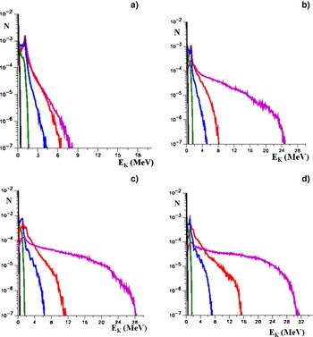
When considering two counter-propagating laser pulses (with P polarization), the wakefield acceleration is overwhelmed when strong stochastic-heating takes place. Figures 28b, 28c, 28d, show that the threshold amplitude of the counter-propagating mode is close to a 1 = 0.1 in good agreement with the value predicted by the single particle approach. Strong stochastic heating is observed when a 1 = 0.3 (Fig. 28d).
(Color online) Electron energy distribution from 1D PIC simulations at different time. P polarization. The plasma slab is 100 µm thick and has a density Ne = 0.01 Nc, tL = 50 τ0. Two semi-infinite laser pulses collide with maximum peak amplitudes a = 3. (a) a1 = 0.01, (b) a1 = 0.1, (c) a1 = 0.2, (d) a1 = 0.3.

The case when the perturbing mode is polarized perpendicularly to the polarization plane of the high intensity wave is also considered (S-polarization) (Bourdier et al., 2005). This polarization rules out electron acceleration due to the Kapitza-Dirac effect (Kapitza & Dirac, 1933; Kotaki et al., 2004). First, the case when a = 3 and a 1 is close to 0.2 was considered. In this case, considering a single particle and many initial conditions, no significant stochastic heating was found (Fig. 29).
(Color online) Average energy of one particle in two waves versus time. S-polarization.  , α = π,
 .
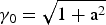 : (a) a = 3.0066, a1 = 0. (b) a = 3, a1 = 0.2. γ0 = 1: (c) a = 3;0066, a1 = 0, (d) a = 3, a1 = 0.2.

No significant stochastic heating is found performing 1D (1Dz3Dv ) PIC code simulation considering the same conditions and parameters as in the previous P-polarization study (Fig. 30).
(Color online) Electron energy distribution from 1D PIC simulations at different times. S-polarization. The plasma slab is 100 µm thick and has a density Ne = 0.01 Nc, tL = 50 τ0. Two semi-infinite laser pulses collide with peak amplitudes. a = 3, a1 = 0.2.

5. CONCLUSION
The dynamic of a charged particle in a linearly or almost linearly polarized traveling high intensity wave that propagates in a medium has been studied. The problem was shown to be integrable when the wave propagates in vacuum. When the wave propagates in plasma, the full plasma response was taken into account by considering plasma wave equations. Until now, the apparent absence of chaos for the system would make it hold pending for the proof of its integrability. Here, an exhaustive and cumbersome numerical work allowed us to see chaotic trajectories in the laboratory frame, showing that the system is not integrable. The same kind of numerical work was achieved in a special Lorentz frame where the variables that describe the waves are space independent. In this frame, at least some chaotic trajectories fill large volumes in phase space. One very important consequence of the nonintegrability of the plasma wave equations is that the Hamilton-Jacobi equation cannot be solved. This implies that, when introducing a perturbing wave in order to generate stochastic heating, one cannot use a classical perturbation method to predict resonances and apply Chirikov criterion.
Then, the wave was assumed to propagate along a constant homogeneous magnetic field in vacuum or in plasma. Two constants, which are canonically conjugate, were found. This property was used to reduce the initially three degrees of freedom problem to two degrees of freedom problem. The system was integrated. Then, in order to study the plasma response in the case of a very high intensity wave propagating in low-density plasma, it was assumed first, that the wave remains linearly polarized. Performing a Lorentz transformation eliminated the space variable corresponding to the direction of propagation of the wave. Just like in the laboratory frame, two canonically conjugate constants were used to reduce the initially three degrees of freedom problem to two degrees of freedom problem. Thus, Poincaré maps are performed. Lyapunov exponents are also calculated to confirm the chaotic nature of some trajectories. Consequently, the system is not integrable and chaos appears when the plasma response is taken into account.
Finally, the interaction of low density plasma with a high intensity plane wave perturbed by a counter-propagating electromagnetic plane wave has been studied. The stability of a single particle interacting with two waves was studied first. The solution of Hamilton-Jacobi equation, in the case of a single particle interacting with one wave, is used to identify resonances. The effect of the different parameters was briefly described by using the Chirikov criterion. Stochastic heating is seen by computing single particle energies. Finally, considering plasma, PIC simulations results obtained with the code CALDER validate the theoretical model for experimentally relevant parameters. Significant stochastic heating can take place in the P-polarization case. Considering the same parameters, no stochastic heating was seen in the S-polarization case. It was shown that a threshold in intensity exists for the low intensity wave when the intensity of the high intensity mode is fixed.