1 Introduction
The flow in rotating drums is of interest for several branches of fluid mechanics when the drum is completely or partially filled with an incompressible Newtonian liquid, a particle-seeded liquid or a granular medium. The importance of these types of flows for industrial applications was first pointed out by Malkin (Reference Malkin1937), who considered the condensation mechanism in paper machine driers. Successive studies extended this work by investigating the transformation of wood pulp into final-stage paper (White Reference White1956; White & Higgins Reference White and Higgins1958). Rotating drums are also employed for carrying coating material in the form of a liquid film (Seiden & Thomas Reference Seiden and Thomas2011), as bio-reactors for solid-state fermentation (Marsh et al. Reference Marsh, Stuart, Mitchell and Howes2000), for rheological measurements (Kaitna & Rickenmann Reference Kaitna and Rickenmann2007a ,Reference Kaitna and Rickenmann b ) and for mixing of granular material (Ottino & Khakhar Reference Ottino and Khakhar2000).
Apart from industrial applications, the rotating drum has become an important configuration to study fundamental phenomena such as instabilities of coating flows and falling films (Yih & Kingman Reference Yih and Kingman1960; Melo Reference Melo1993; Thoroddsen & Mahadevan Reference Thoroddsen and Mahadevan1997; Vallette, Jacobs & Gollub Reference Vallette, Jacobs and Gollub1997; Hosoi & Mahadevan Reference Hosoi and Mahadevan1999). Compared to other flow configurations, the rotating drum offers the advantage of a confined set-up, which, in the case of infinite axial extension, allows for strictly periodic flows. Therefore, the flow in a rotating drum partially filled with a Newtonian liquid has been extensively studied experimentally, theoretically and numerically (Phillips Reference Phillips1960; Balmer Reference Balmer1970; Moffatt Reference Moffatt1977; Orr & Scriven Reference Orr and Scriven1978; Lin Reference Lin1986; Matson, Ackerson & Tong Reference Matson, Ackerson and Tong2003; Thoroddsen & Tan Reference Thoroddsen and Tan2004; Chen et al. Reference Chen, Tsai, Liu and Wu2007). Of primary interest have been the different hydrodynamic instabilities of rimming flows involving substantial interfacial deformations and the existence ranges of different types of flows as a function of the Reynolds, Froude and capillary numbers, the viscosity ratio and the filling ratio, which is defined as the ratio of the volume occupied by the fluid to the total cylindrical volume of the drum. A multitude of flow patterns have been observed between the two extremes of a liquid pool at low Reynolds numbers and a coating film at high Reynolds numbers. The patterns range from hygrocysts (Balmer Reference Balmer1970) over sloshing, shark-teeth interfaces, metastable states, counter-flowing jets and hydraulic jumps to fluid curtains and fingering instabilities (Thoroddsen & Mahadevan Reference Thoroddsen and Mahadevan1997; Thoroddsen & Tan Reference Thoroddsen and Tan2004).
In the present work we investigate the three-dimensional flow in a partially liquid-filled rotating drum in the limit in which the liquid–gas interface remains flat and perpendicular to the gravity vector. We compute finite-amplitude axially periodic steady flows for an infinitely extended cylinder. These flows arise in the form of steady cells for Reynolds numbers beyond the first critical value at which the axial translation invariance is broken. Such periodic flows also dominate the flow in long but finite-size systems (see e.g. Neitzel Reference Neitzel1984; Siegmann-Hegerfeld, Albensoeder & Kuhlmann Reference Siegmann-Hegerfeld, Albensoeder and Kuhlmann2008) found in applications, except for a region near the endwalls. Attention is focused on the unknown streamline structure and the location of regular and chaotic regions of the flow. These flow properties are of key importance for the transport of particles with a small density mismatch relative to the fluid and their accumulation by particle–boundary interactions (Mukin & Kuhlmann Reference Mukin and Kuhlmann2013; Romanò, Albensoeder & Kuhlmann Reference Romanò, Albensoeder and Kuhlmann2017). Moreover, the mixing properties of the flow are important for rheological measurements utilising rotating drums (Kaitna & Rickenmann Reference Kaitna and Rickenmann2007a ,Reference Kaitna and Rickenmann b ).
In the limit considered, the partially filled rotating drum corresponds to a driven cavity bounded by a flat stress-free surface and a circular arch in steady tangential motion. Several studies of chaotic advection have been carried out for cavity flows driven by tangentially moving walls. Most of these were concerned with time-dependent two-dimensional flows in the Stokes-flow regime, because the computational cost required for investigating chaotic advection in spatially three-dimensional Navier–Stokes flows is very high, even for steady flows. Topological studies of other flow systems have mostly been carried out for conditions in which either a marching technique in time can be used (Oteski et al. Reference Oteski, Duguet, Pastur and Quéré2015; Contreras, de la Cruz & Ramos Reference Contreras, de la Cruz and Ramos2016), for which closed-form solutions of the Navier–Stokes or the Euler equations are available (ABC flow; Dombre et al. Reference Dombre, Frisch, Greene, Hénon, Mehr and Soward1986; Haller Reference Haller2001), or for Stokes flows, which can be constructed using the superposition principle (see e.g. Kroujiline & Stone Reference Kroujiline and Stone1999). The topology of a non-trivial Stokes flow was investigated by Speetjens, Clercx & Heijst (Reference Speetjens, Clercx and Van Heijst2004). They computed and measured the transport in a finite-length cylinder in which the creeping flow was induced by tangential motion of the plane bounding endwalls according to a different time protocol. Depending on the protocol for the wall motion, they classified three fundamental states of tracer motion, being non-chaotic, two-dimensional locally chaotic or three-dimensional globally chaotic. Other studies have been conducted for model flows obtained by perturbation expansions in which weak nonlinearities induce the chaotic advection (for Rayleigh–Bénard convection, see e.g. Arter (Reference Arter1983) and Chernikov & Schmidt (Reference Chernikov and Schmidt1992)). Using an analytical model, Broomhead & Ryrie (Reference Broomhead and Ryrie1988) found chaotic flow regions at the onset of wavy vortices in the Taylor–Couette problem, which they related to the breakup of heteroclinic connections between two hyperbolic points on the cylindrical walls separating individual Taylor vortices.
Only a limited number of investigations are available based on three-dimensional flow computations. An early example is the work of Rudman (Reference Rudman1998), who considered the numerical solution of the Navier–Stokes equations for fully nonlinear wavy Taylor-vortex flows, extending the work of Broomhead & Ryrie (Reference Broomhead and Ryrie1988). They characterised the chaotic mixing by an axial diffusion coefficient and investigated the effect of the chaotic mixing on the axial dispersion of settling of inertial particles. Other examples of chaotic mixing in numerical three-dimensional Navier–Stokes flows have been reported only recently. Sotiropoulos, Ventikos & Lackey (Reference Sotiropoulos, Ventikos and Lackey2001) considered the flow in a cylinder driven by a rotating lid. The onset of chaotic motion was traced back to Shil’nikov’s mechanism (Shil’nikov Reference Shil’nikov1965) by which the heteroclinic connection of the two free stagnation points of the vortex breakdown bubble in two-dimensional flows is destroyed by three-dimensional flow perturbations. Mukin & Kuhlmann (Reference Mukin and Kuhlmann2013) investigated the flow in a thermocapillary liquid bridge after the onset of a three-dimensional hydrothermal wave. They identified very slender Kolmogorov–Arnold–Moser (KAM) tori for different Reynolds numbers and discussed the implications of the flow topology with respect to particle transport and accumulation. Romanò et al. (Reference Romanò, Albensoeder and Kuhlmann2017) computed the flow structure in a two-sided lid-driven cavity and analysed its Lagrangian structure. The breakup of a degenerate heteroclinic connection and the abundance of complex saddle foci was identified as the origin of chaos, which sets in globally just above the threshold to the three-dimensional flow. With a perspective towards applications, Speetjens et al. (Reference Speetjens, Demissie, Metcalfe and Clercx2014) studied inline mixing by rotating arc mixers. In these systems the fluid is driven through a straight pipe with periodic windows in the wall at which the fluid is exposed to an azimuthal wall motion realised by an outer rotating cylinder snugly fitted to the pipe. The authors characterised the nature of the mixing by computing the flow topology including fluid inertia.
Apart from clarifying the local and global transport in the present partially filled rotating drum, our investigation is also motivated by the importance of the regions of regular versus chaotic streamlines for the transport and accumulation of finite-size non-inertial particles when their motion is affected by boundaries (Hofmann & Kuhlmann Reference Hofmann and Kuhlmann2011; Mukin & Kuhlmann Reference Mukin and Kuhlmann2013; Muldoon & Kuhlmann Reference Muldoon and Kuhlmann2016). The novelty of this particle accumulation phenomenon is that it does not rely on particle inertia, but only on the particle size. This class of coherent structures has originally been found in thermocapillary flows (Schwabe, Hintz & Frank Reference Schwabe, Hintz and Frank1996) and has recently been reported for a mechanically driven system (Kuhlmann et al. Reference Kuhlmann, Romanò, Wu, Albensoeder, Ivey, Zhou, Jones and Draper2016). In boundary-driven flows certain KAM tori can be located very close to the moving boundary such that particles can be transferred from chaotic to regular regions of the flow by way of particle–boundary collisions, leading to a trapping of particles inside the regular flow structures. Therefore, an understanding of this particle accumulation mechanism (Schwabe et al. Reference Schwabe, Hintz and Frank1996; Kuhlmann et al. Reference Kuhlmann, Romanò, Wu, Albensoeder, Ivey, Zhou, Jones and Draper2016) requires an accurate description of the flow topology.
The incompressible flow in a partially liquid-filled horizontally rotating drum has not received much attention for the case in which a liquid pool at the bottom of the cavity is formed. We compute the nonlinear three-dimensional flow for a ratio of pool depth to radius of
 $h=0.2$
in the limit in which the free liquid–gas interface is plane and non-deformable. In § 2 the problem under investigation is formulated mathematically. Section 3 presents the numerical methods used to simulate the fluid flow and to characterise its streamlines. Results in terms of KAM structures and Lagrangian chaos in the steady three-dimensional cellular flow are presented in § 4. Conclusions are drawn in § 5, in which the results are also compared with other fluid-dynamical systems.
2 Problem formulation
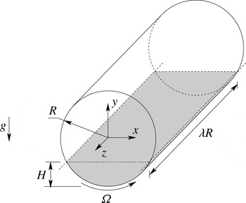
A drum with circular cross-section of radius
 $R$
is partially filled with an incompressible Newtonian liquid of constant density
 $\unicode[STIX]{x1D70C}$
and kinematic viscosity
 $\unicode[STIX]{x1D708}$
and with a passive gas. The cylindrical cavity is assumed to be infinitely extended in the horizontal
 $z$
-direction with the acceleration of gravity
 $g$
acting perpendicular to the axis. When the liquid and the drum are at rest, the maximum liquid depth is
 $H$
. The flow is driven by rotation of the drum about its axis with constant angular velocity
 $\unicode[STIX]{x1D6FA}$
. Figure 1 shows a sketch of the set-up.
Sketch of the partially filled rotating drum. The region in grey represents the liquid phase.

The problem is governed by the Reynolds, capillary and Froude numbers (Thoroddsen & Mahadevan Reference Thoroddsen and Mahadevan1997)
 $$\begin{eqnarray}Re=\frac{\unicode[STIX]{x1D6FA}R^{2}}{\unicode[STIX]{x1D708}},\quad Ca=\frac{\unicode[STIX]{x1D70C}\unicode[STIX]{x1D708}\unicode[STIX]{x1D6FA}R}{\unicode[STIX]{x1D70E}},\quad Fr=\frac{\unicode[STIX]{x1D6FA}^{2}R}{g},\end{eqnarray}$$
where
 $\unicode[STIX]{x1D70E}$
is the surface tension, and by the normalised pool depth
 $h=H/R$
. We consider the limit in which gravity forces dominate over centrifugal and capillary forces and in which capillary forces dominate over inertia forces. This requires
 $Fr\ll 1$
,
 $Fr/(CaRe)\ll 1$
and
 $CaRe\ll 1$
, respectively, and leads to the dedicated limit
 $Fr,Ca\rightarrow 0$
with
 $Fr/Ca\rightarrow 0$
such that
 $Re=O(1)$
. In the asymptotic limit, the interface remains flat and perpendicular to the gravity vector, and the meniscus near the contact line can be neglected.
The above conditions are approximately met when the rotation rate is sufficiently small and the radius and the surface tension are large. For instance, in a drum with
 $R=3.25~\text{cm}$
and axial length
 $L=48.75~\text{cm}$
using a 20 cSt silicone oil filled up to
 $H=1.85~\text{cm}$
we experimentally observed an essentially flat interface safely up to
 $Re=2500$
. The liquid film pulled out of the pool was very thin. Numerical volume-of-fluid (VOF) simulations of the combined liquid–gas flow confirmed the interface to be flat except for small menisci near the contact line (Hajisharifi Reference Hajisharifi2016).
In the dedicated limit, the flow in the liquid phase is governed by the Navier–Stokes and continuity equations,
 $$\begin{eqnarray}\displaystyle & \displaystyle (\unicode[STIX]{x2202}_{t}+\boldsymbol{u}\boldsymbol{\cdot }\unicode[STIX]{x1D735})\boldsymbol{u}=-\unicode[STIX]{x1D735}p+Re^{-1}\unicode[STIX]{x1D6FB}^{2}\boldsymbol{u}, & \displaystyle\end{eqnarray}$$
 $$\begin{eqnarray}\displaystyle & \displaystyle \unicode[STIX]{x1D735}\boldsymbol{\cdot }\boldsymbol{u}=0, & \displaystyle\end{eqnarray}$$
 $\boldsymbol{u}=(u,v,w)$
and
 $p$
are the velocity vector with Cartesian components and the pressure, respectively, and
 $t$
and
 $\boldsymbol{x}=(x,y,z)$
denote the temporal and spatial Cartesian coordinates. Alternatively, cylindrical coordinates
 $(r,\unicode[STIX]{x1D711},z)$
are used in which
 $z$
is directed parallel to the cylinder’s axis. The common origin of both coordinate systems is located on the axis and the unit vectors
 $\boldsymbol{e}_{x}$
and
 $\boldsymbol{e}_{y}$
are, respectively, oriented parallel and perpendicular to the interface as shown in figure 1. Equations (2.2) have been made dimensionless using the scales
 $R$
,
 $\unicode[STIX]{x1D6FA}^{-1}$
,
 $\unicode[STIX]{x1D6FA}R$
and
 $\unicode[STIX]{x1D70C}\unicode[STIX]{x1D6FA}^{2}R^{2}$
for lengths, time, velocity and pressure, respectively.
To close the problem, no-slip and no-penetration boundary conditions are enforced along the moving wall. Owing to the small viscosity of the gas as compared to the liquid, free-stress boundary conditions are imposed on the flat interface, leading to
 $$\begin{eqnarray}\displaystyle & \displaystyle r=1:\quad \boldsymbol{u}=\boldsymbol{e}_{\unicode[STIX]{x1D711}}, & \displaystyle\end{eqnarray}$$
 $$\begin{eqnarray}\displaystyle & \displaystyle y=h-1:\quad v=\frac{\unicode[STIX]{x2202}u}{\unicode[STIX]{x2202}y}=\frac{\unicode[STIX]{x2202}w}{\unicode[STIX]{x2202}y}=0. & \displaystyle\end{eqnarray}$$
 $h=0.2$
, the basic flow becomes unstable to a spatially periodic steady three-dimensional cellular flow with wavelength
 $\unicode[STIX]{x1D706}_{c}$
, which exhibits mirror-symmetry planes at
 $z=\text{const.}$
on which
 $w=0$
. In order to investigate the properties of the steady supercritical flow, we restrict the analysis to periodic boundary conditions:
 $$\begin{eqnarray}\boldsymbol{u}(z=\unicode[STIX]{x1D706}_{c}/2)=\boldsymbol{u}(z=-\unicode[STIX]{x1D706}_{c}/2).\end{eqnarray}$$
3 Methods of investigation
3.1 Fluid flow
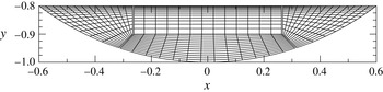
The numerical simulations are carried out using the collocated finite-volume solver icoFoam included in the open-source software package OpenFOAM. The domain is discretised such that each cross-section encompasses 67 600 finite volumes, distributed in the
 $(x,y)$
-plane as shown in figure 2. In the
 $z$
-direction 450 equidistant layers of finite volumes are used, resulting in a total of approximately 31 million finite volumes.
Standard second-order discretisation schemes are employed in both space and time. Spatial derivatives are treated using central schemes, while time is advanced implicitly (backward of OpenFOAM). The PISO algorithm is adjusted to involve two correction steps, each of which is internally corrected twice to take care of the non-orthogonality of the grid (nCorrectors=2 and nNonOrthogonalCorrectors=2). The resulting algebraic systems are all solved using iterative relaxation methods. The relative residuals are required to be less than
 $10^{-7}$
. For the momentum equation the selected iterative solver is based on the symmetric Gauss–Seidel method, whereas for the pressure-projection step a geometric–algebraic multi-grid Gauss–Seidel solver is adopted.
Distribution of the computational cells in the
 $(x,y)$
-plane for each cross-section. The double lines indicate the blockMesh boundaries defined in OpenFOAM. Unless noted otherwise, the grid for the simulation is 10 times finer than the one shown.

For the temporal discretisation a time step of
 $\unicode[STIX]{x0394}t=10^{-5}$
is used. Time stepping is continued up to steadiness, which is assumed once the termination criterion
 $$\begin{eqnarray}\max _{\boldsymbol{x},i}\frac{|u_{i}(\boldsymbol{x},t)-u_{i}(\boldsymbol{x},t-\unicode[STIX]{x0394}t)|}{\unicode[STIX]{x0394}t}\leqslant 10^{-7}\end{eqnarray}$$
is satisfied.
For cavity-type flows OpenFOAM has been well verified (see also Mukin & Kuhlmann Reference Mukin and Kuhlmann2013). Moreover, grid convergence has been obtained for all supercritical Reynolds numbers considered.
3.2 Streamlines
The streamline topology of the three-dimensional steady cellular flow is calculated by integrating the advection equation. Denoting with
 $\boldsymbol{X}$
the position of a fluid particle, its motion is governed by
 $$\begin{eqnarray}\displaystyle \frac{\text{D}\boldsymbol{X}}{\text{D}t}=\boldsymbol{u}(\boldsymbol{X}),\end{eqnarray}$$
with initial condition
 $\boldsymbol{X}(t=0)=\boldsymbol{X}_{0}$
.
A Runge–Kutta Dormand–Prince method (Dormand & Prince Reference Dormand and Prince1980) is employed for the integration of (3.2). It is based on fourth- and fifth-order Runge–Kutta schemes and uses the difference between the two solutions to estimate the integration error at each time step. The time step
 $\unicode[STIX]{x0394}t$
is adaptive to ensure that the predicted absolute and relative numerical errors are always less than
 $10^{-7}$
. The flow-field interpolation required for evaluating
 $\boldsymbol{u}(\boldsymbol{X})$
is obtained consistently with the order of accuracy of the finite-volume method, i.e. quadratic on each element of the discretisation.
4 Results
4.1 Critical conditions
In order to determine the critical conditions at which the basic flow becomes unstable to three-dimensional perturbations, three-dimensional simulations have been carried out for different Reynolds numbers
 $Re$
and wavelengths
 $\unicode[STIX]{x1D706}$
. For these simulations, a relatively coarse grid was used, which was only twice as fine as the one shown in figure 2 using 50 finite volumes in the
 $z$
-direction. All simulations were extended until a steady state was reached. From the steady states, the maximum
 $A=\max _{z}w(x_{0},y_{0},z)$
of
 $w(z)$
was determined along the ray
 $(x_{0},y_{0})=(0,-0.95)$
. The maxima of
 $w(z)$
for
 $Re=900$
, 1000 and 1250 have been fitted, for each wavelength
 $\unicode[STIX]{x1D706}$
, to the square-root law
 $A=c\sqrt{Re-Re_{n}}$
using least squares. From these fits the neutral curve
 $Re_{n}(\unicode[STIX]{x1D706})$
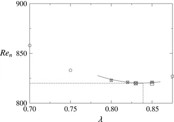
was obtained. The result is shown in figure 3. A quadratic best fit to the neutral Reynolds numbers yields the critical point
 $(Re_{c},\unicode[STIX]{x1D706}_{c})=(820\pm 50,0.839\pm 0.01)$
. To check the accuracy of this result, the simulations are repeated for two values of
 $\unicode[STIX]{x1D706}$
, doubling the mesh size in each direction. The finer-resolution results are shown in figure 3 as squares, essentially confirming the low-resolution results. Since we aim at the nonlinear supercritical flow and not at a linear stability analysis, for which numerical simulation is not the method of choice due to the critical slowing down, we did not further refine the mesh. Based on the results obtained, the period of the flow is fixed to
 $\unicode[STIX]{x1D706}_{c}=0.839$
in order to study the topology of the supercritical flow at higher Reynolds numbers using a much higher grid resolution.
Neutral Reynolds numbers
 $Re_{n}$
(symbols) obtained from square-root fits of the maxima of
 $w(x_{0}=0,y_{0}=-0.95,z)$
for constant
 $\unicode[STIX]{x1D706}$
and Reynolds numbers
 $Re=900$
,
 $1000$
and
 $1250$
. The neutral curve is approximated by a quadratic fit (full line) to the four smallest neutral Reynolds number (crosses). Squares represent neutral Reynolds numbers obtained on the refined mesh and dashed lines indicate
 $\unicode[STIX]{x1D706}_{c}$
and
 $Re_{c}$
.

4.2 General structure of the flow field
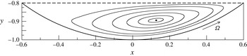
The two-dimensional steady basic flow
 $\boldsymbol{u}_{0}(x,y)$
arises as a single vortex. Owing to inertia, its centre is slightly shifted downstream of the moving cylindrical wall. As an example, we show in figure 4 the near-critical flow structure at
 $Re=780$
, which is within the error margins of the critical Reynolds number.
Streamlines of the basic two-dimensional flow at
 $Re=780$
, very close to criticality. The dot indicates the elliptic point at the vortex centre. The dashed line marks the stress-free surface.

At
 $Re=820\pm 50$
the flow becomes three-dimensional via a steady supercritical pitchfork bifurcation. The saturated steady perturbation flow
 $\boldsymbol{u}(x,y,z)$
is characterised by pairs of vortices, periodic in
 $z$
, which are primarily aligned with the
 $x$
-axis. In a system infinitely extended in
 $z$
, such steady bifurcating flows have periodic mirror-symmetry planes at
 $z=\text{const.}$
, which are equally spaced at a distance
 $\unicode[STIX]{x0394}z=\unicode[STIX]{x1D706}/2$
. Therefore, calculations have been carried out using the periodic boundary conditions (2.4), enforcing
 $\unicode[STIX]{x1D706}=\unicode[STIX]{x1D706}_{c}$
. One period of the flow field comprises two mirror-symmetric convection cells. We restrict the discussion to the flow within a single cell bounded by two neighbouring symmetry planes and occupying the interval
 $z\in [-\unicode[STIX]{x1D706}_{c}/4,\unicode[STIX]{x1D706}_{c}/4]$
. The mirror-symmetry planes
 $z=\pm \unicode[STIX]{x1D706}_{c}/4$
on which the axial velocity vanishes
 $(w=0)$
represent barriers to the transport. The two-dimensional flow
 $(u,v)$
on these cell boundaries is not incompressible.
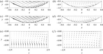
Projection of the velocity vectors for
 $Re=1000$
onto the planes
 $z=-\unicode[STIX]{x1D706}/4$
(a,b),
 $z=\unicode[STIX]{x1D706}/4$
(c,d) and
 $x=0.2$
(e,f). Panels (a,c,e) show the full three-dimensional flow, whereas panels (b,d,f) show the deviation from the two-dimensional part of the flow, i.e. from the average in the
 $z$
-direction
 $(2/\unicode[STIX]{x1D706})\int _{-\unicode[STIX]{x1D706}/4}^{\unicode[STIX]{x1D706}/4}\boldsymbol{u}\,\text{d}z$
.

An example of the three-dimensional flow field is given in figure 5 for
 $Re=1000$
. Figure 5(a,c,e) shows the structure of the full flow field
 $\boldsymbol{u}$
in different planes. Figure 5(b,d,f) shows the deviation (perturbation) from the two-dimensional part of the flow, i.e.
 $\boldsymbol{u}-(2/\unicode[STIX]{x1D706})\int _{-\unicode[STIX]{x1D706}/4}^{\unicode[STIX]{x1D706}/4}\boldsymbol{u}\,\text{d}z$
. The perturbation flow in the planes
 $z=\pm \unicode[STIX]{x1D706}_{c}/4$
(figure 5
b,d) arises as a vortex with the opposite sense of rotation to the two-dimensional basic vortex (not shown, but see figure 4). The location of the apparent vortex centre of the full three-dimensional flow in these planes (figure 5
a,c) is significantly influenced by the three-dimensional perturbation flow: the vortex centre at
 $z=\unicode[STIX]{x1D706}_{c}/4$
is located quite close to and downstream of the moving cylinder. The vortex centre at
 $z=-\unicode[STIX]{x1D706}_{c}/4$
is less affected. Moreover, at
 $x=0.2$
, there is a strong downwelling between the two convection cells at
 $z=\unicode[STIX]{x1D706}/4$
(figure 5
e,f) as a result of the perturbation vorticity in the
 $x$
-direction. Note that the perturbation vortex in planes
 $x=\text{const.}$
changes the sense of rotation depending on
 $x$
.
The qualitative features of the supercritical flow discussed are very robust. The apparent centre of the perturbation vortex flow in the plane
 $x=0.2$
moves closer to the mirror-symmetry plane
 $z=\unicode[STIX]{x1D706}/4$
as the Reynolds number is increased. In the following, the three-dimensional flow is analysed in more detail for five supercritical Reynolds numbers,
 $Re=900$
, 950, 1000, 1500 and 2000.
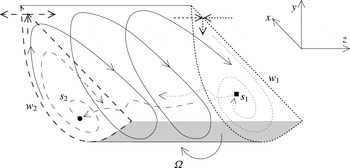
Sketch of the topological elements of the supercritical flow in a partially filled rotating drum. Shown are the spiralling-in (square) and spiralling-out (circle) saddle foci with fixed points
 $s_{1}$
and
 $s_{2}$
, respectively, the corresponding one-dimensional unstable and stable manifolds, and the saddle limit cycles
 $w_{1}$
on
 $z=\unicode[STIX]{x1D706}/4$
(dotted line) and
 $w_{2}$
on
 $z=-\unicode[STIX]{x1D706}/4$
(dashed line).

4.3 Broken heteroclinic connection
The supercritical flow in a periodic cell is typically organised around two critical points, two limit cycles, and their respective stable and unstable manifolds as sketched in figure 6. The critical points are the two free stagnation points
 $s_{1}$
and
 $s_{2}$
on the cell boundaries at
 $z=\pm \unicode[STIX]{x1D706}/4$
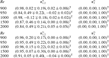
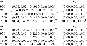
. Their coordinates are provided in table 1. The critical points are double spiralling-in
 $(z=+\unicode[STIX]{x1D706}/4)$
and double spiralling-out
 $(z=-\unicode[STIX]{x1D706}/4)$
saddle foci. This is confirmed by the eigenvalues of the velocity-gradient tensor at the critical points, which are also listed in table 1. The corresponding normalised eigenvectors of the velocity-gradient tensor at the saddle foci are provided in table 2.
Location of the stagnation points
 $s_{1,2}$
and corresponding eigenvalues
 $\unicode[STIX]{x1D706}_{i}$
(
 $i=1,2,3$
) of the velocity-gradient tensor.

Normalised eigenvectors
 $\boldsymbol{v}_{i}$
of the velocity-gradient tensor at the two saddle foci
 $s_{1,2}$
on the cell boundaries.
The limit cycles are saddle limit cycles on the edges of the two cell boundaries, which are attracting on the cell boundary
 $z=-\unicode[STIX]{x1D706}/4$
and repelling on
 $z=+\unicode[STIX]{x1D706}/4$
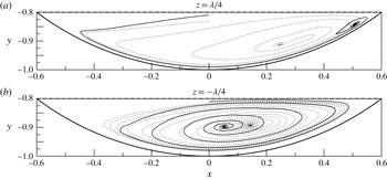
. The inward- and outward-spiralling motion on the cell boundaries at
 $z=\pm \unicode[STIX]{x1D706}/4$
is shown in figure 7 for
 $Re=1000$
and
 $Re=2000$
. The saddle limit cycles are degenerate and of higher order, because the stable manifold of the limit cycle on
 $z=+\unicode[STIX]{x1D706}/4$
and the unstable manifold of the limit cycle on
 $z=-\unicode[STIX]{x1D706}/4$
are made of the cylindrical wall and the free surface.
Spiralling-in (a) and spiralling-out (b) motion on the cell boundary towards and from the saddle focus, respectively, for
 $Re=2000$
(full line) and
 $Re=1000$
(dotted).

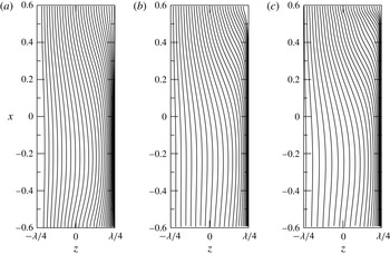
Streamlines on the free surface for
 $Re=1000$
(a),
 $1500$
(b) and
 $2000$
(c). The flow direction is from top to bottom.

For
 $Re>Re_{c}$
fluid is transported in the
 $z$
-direction. From the real eigenvalues of the saddle foci it is clear that for
 $Re\geqslant 950$
fluid is transported in the bulk in the negative
 $z$
-direction from the cell boundary at
 $z=+\unicode[STIX]{x1D706}/4$
to the cell boundary at
 $z=-\unicode[STIX]{x1D706}/4$
(figure 5
f). This transport is compensated by a transport along the two-dimensional manifold heteroclinically connecting the two limit cycles. While the transport along the cylindrical wall is purely azimuthal, the transport in the
 $z$
-direction along the manifold is determined by the free-surface flow. From the streamlines in figure 8, the net transport of fluid elements along the free surface from the contact line at
 $x=0.6$
to the one at
 $x=-0.6$
is always in the positive
 $z$
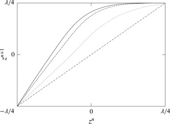
-direction. The map
 $z^{n+1}=P(z^{n})$
of the
 $z$
-coordinate of a fluid element between the two contact lines and along the free surface is shown in figure 9 for the three Reynolds numbers
 $\mathit{Re}=1000,1500,2000$
. For each map, only two fixed points exist at
 $z=\pm \unicode[STIX]{x1D706}/4$
corresponding to the saddle limit cycles on the cell boundaries.
Mapping from edge to edge of the
 $z$
-coordinates connected by streamlines on the free surface for
 $Re=1000$
(dotted line),
 $1500$
(dashed line) and
 $2000$
(solid line). The dashed–dotted line indicates the bisector.

The transport in the bulk is more complicated, because the one-dimensional stable and unstable manifolds of the saddle foci at
 $z=-\unicode[STIX]{x1D706}/4$
and
 $z=+\unicode[STIX]{x1D706}/4$
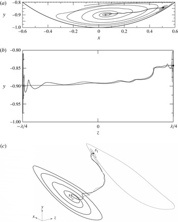
, respectively, are distinct for all supercritical Reynolds numbers investigated. As an example, approximations to the one-dimensional manifolds of both saddle foci are shown in figure 10 for
 $Re=2000$
. They have been obtained by integrating (3.2) forwards and backwards in time for a time span
 $T$
using as initial conditions
 $\boldsymbol{X}_{0}$
the best estimates of the saddle focus points
 $\boldsymbol{x}_{s_{1}}$
and
 $\boldsymbol{x}_{s_{2}}$
, respectively. As the Reynolds number is decreased, the two manifolds approach each other. Thus they are expected to merge at
 $Re=Re_{c}$
to a degenerate heteroclinic connection made of an infinite sequence of elliptic points. In this sense, the two distinct manifolds for
 $Re>Re_{c}$
represent a broken heteroclinic connection.
The topology is richer for
 $Re=900$
. At this comparatively low Reynolds number, we find an additional free stagnation point near the cell boundary at
 $z=-\unicode[STIX]{x1D706}/4$
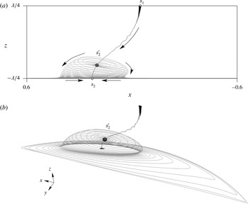
. Characteristic streamlines are shown in figure 11. The new stagnation point
 $s_{2}^{\prime }$
, which is a spiralling-out saddle focus, is located downstream of the one-dimensional unstable manifold of the spiralling-in saddle focus
 $s_{1}$
. The unstable two-dimensional manifold of the spiralling-out saddle focus is found to end on the cell boundary at
 $z=-\unicode[STIX]{x1D706}/4$
, demarcating a separation bubble. The locus where the manifold ends on the cell boundary is a saddle limit cycle
 $w_{b}$
(see grey line in figure 13). As a result the singular point
 $s_{2}$
is a spiralling-in saddle focus for
 $Re=900$
. Within the numerical accuracy
 $s_{1}$
and
 $s_{2}^{\prime }$
are not connected with each other (figure 11). Whether or not
 $s_{2}$
and
 $s_{2}^{\prime }$
are connected cannot be definitely clarified. It is known, however, that homoclinic connections such as
 $s_{2}$
–
 $s_{2}^{\prime }$
–
 $w_{b}$
are structurally unstable (Arneodo, Coullet & Tresser Reference Arneodo, Coullet and Tresser1982; Gaspard & Nicolis Reference Gaspard and Nicolis1983).
One-dimensional unstable and stable manifolds of the spiralling-in (
 $s_{1}$
, square, black line,
 $T=50$
) and spiralling-out (
 $s_{2}$
, dot, grey line,
 $T=30$
) saddle focus, respectively, for
 $Re=2000$
. Shown are projections onto the
 $(x,y)$
-plane (a) and
 $(y,z)$
-plane (b). A three-dimensional view of the broken connection is shown in (c).

One-dimensional stable (black line) and unstable (grey line) manifolds of the spiralling-out saddle focus (
 $s_{2}^{\prime }$
, marker) for
 $Re=900$
. Shown are projections onto the
 $(x,z)$
-plane (a) and a three-dimensional visualisation (b).

The clear distinction of the one-dimensional manifolds of
 $s_{1}$
and
 $s_{2}$
for
 $Re\geqslant 950$
and of
 $s_{1}$
and
 $s_{2}^{\prime }$
for
 $Re=900$
together with the global recirculating flow structure provides a return mechanism for fluid elements that is highly sensitive to the initial conditions in the vicinity of the hyperbolic points. Therefore, chaotic streamlines are expected to grow from the broken connection and from the boundaries.
4.4 KAM tori and chaotic sea
The steady three-dimensional supercritical flow corresponds to the flux in phase space of a Hamiltonian system with 1.5 degrees of freedom (Bajer Reference Bajer1994). Therefore, chaotic and regular regions may coexist depending on the system and flow parameters. The regular regions arise as KAM tori (Ottino Reference Ottino1989; Schuster Reference Schuster2005). Since the region occupied by chaotic streamlines typically grows from the boundaries (Arter Reference Arter1983; Aref Reference Aref2002; Biemond et al. Reference Biemond, de Moura, Károlyi, Grebogi and Nijmeijer2008) and from the broken heteroclinic connection, the KAM tori will shrink as the Reynolds number is increased from its critical value for the onset of three-dimensional flow.
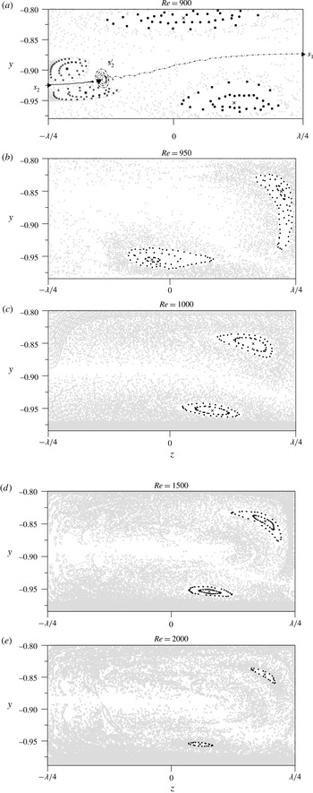
Poincaré sections on
 $x=0.2$
of streamlines for
 $Re=900$
(a) and on
 $x=0.15174$
for
 $Re=950$
(b), 1000 (c), 1500 (d) and 2000 (e). Poincaré points for streamlines on KAM tori are shown as black symbols, and points for chaotic streamlines are shown in grey. The simply periodic closed orbits inside the KAM tori are marked by a cross or an asterisk. The dashed–dotted and solid lines in (a) are projections of the one-dimensional manifolds emerging from
 $s_{1}$
and
 $s_{2}$
, respectively. Saddle foci are shown as full triangles.

To find the KAM tori, we consider a total of 1000 streamlines initialised in the plane
 $x=0$
very close to the rotating cylinder. The initial points are equidistantly spaced in
 $z\in [-\unicode[STIX]{x1D706}/4,\unicode[STIX]{x1D706}/4]$
with 200 points on each of the five rays
 $(x,y)=(0,-1+n\times 10^{-4})$
, where
 $n=1,2,3,4,5$
. The trajectories are integrated up to
 $t=50$
and classified as either chaotic or regular by means of Poincaré sections. Once a KAM torus has been identified from a trajectory, it is computed more accurately using a smaller error tolerance. In such a case the absolute and relative tolerances of the Dormand–Prince scheme are reduced to
 $10^{-9}$
and the maximum time step size is constrained to
 $\unicode[STIX]{x0394}t\leqslant 10^{-6}$
.
For Reynolds numbers
 $Re\geqslant 950$
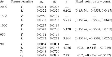
only a single set of nested KAM tori could be identified. The higher the Reynolds number, the smaller the regular regions become. The largest reconstructible KAM tori are illustrated in figure 12(b–e) by Poincaré sections on the plane
 $x=0.15174$
for
 $Re=950$
, 1000, 1500 and 2000. For these Reynolds numbers, the KAM tori are located in the same region
 $z>0$
and in proximity of the spiralling-in saddle focus. In all cases the largest KAM torus approaches the boundaries closely, always passing the free surface closer than the rotating wall.
For
 $Re=900$
, we use 50 dedicated initial conditions to create a Poincaré section on
 $x=0.2$
. The result is shown in figure 12(a). Owing to the separated region, two sets of KAM tori exist. Both regular regions are much larger than the regular regions found at higher Reynolds numbers. Apart from the expected chaotic region around the broken connection between
 $s_{1}$
and
 $s_{2}^{\prime }$
, we find a clear but relatively narrow chaotic region between
 $s_{2}$
and
 $s_{2}^{\prime }$
.
To further characterise the regular regions, the closed streamlines inside of the KAM tori are calculated for each Reynolds number. They play a key role in the accumulation of finite-size particles (Mukin & Kuhlmann Reference Mukin and Kuhlmann2013; Kuhlmann et al.
Reference Kuhlmann, Romanò, Wu, Albensoeder, Ivey, Zhou, Jones and Draper2016). A Newton–Raphson method was employed to localise one of the two elliptic fixed points in the Poincaré plane at
 $x=0.15174$
. The iteration was terminated when the distance between two successive Poincaré points became less than
 $10^{-4}$
.
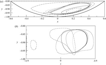
Projections of the closed streamlines onto the
 $(x,y)$
- and
 $(y,z)$
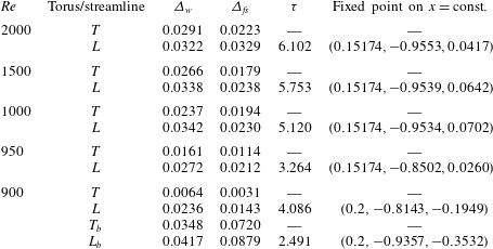
-planes are shown in figure 13. The minimum distances of the closed streamlines from the free surface and the rotating wall, the fixed points in the plane at
 $x=\text{const.}$
and the periods
 $\unicode[STIX]{x1D70F}$
of the closed orbits are listed in table 3.
Simply periodic closed streamlines projected to the plane
 $z=0$
(a) and
 $x=0$
(b). The double dotted–dashed, dotted–dashed, dotted, dashed and solid lines refer to
 $Re=900$
, 950, 1000, 1500 and 2000, respectively. The grey line denotes the saddle limit cycle
 $w_{b}$
on the cell boundary.

Minimum distance of the largest reconstructible KAM surface
 $T$
and of the closed streamline
 $L$
from the moving wall
 $(\unicode[STIX]{x1D6E5}_{w})$
and from the free surface
 $(\unicode[STIX]{x1D6E5}_{fs})$
. Also listed are the turnover time
 $\unicode[STIX]{x1D70F}$
of the periodic orbit and one of its two fixed points in the Poincaré plane
 $x=\text{const}$
. The subscript
 $b$
refers to the KAM torus inside the separation bubble near the cell boundary.
5 Discussion and conclusions
The topology of the steady three-dimensional flow in a partially filled horizontal rotating drum has been investigated for a ratio of pool depth to radius of
 $h=0.2$
. By a series of numerical simulations, the critical conditions for the onset of three-dimensional flow in an infinitely extended drum were obtained as
 $Re_{c}=820\pm 50$
and
 $\unicode[STIX]{x1D706}_{c}=0.839\pm 0.01$
. Accurate spatially periodic supercritical flows were calculated for Reynolds numbers
 $Re=900$
, 950, 1000, 1500 and 2000, fixing the wavelength to
 $\unicode[STIX]{x1D706}=\unicode[STIX]{x1D706}_{c}$
.
The supercritical flows arise in the form of steady cellular convection cells. The convection cells are separated by mirror-symmetry planes at constant
 $z$
on which
 $w=0$
. For large Reynolds number,
 $Re\geqslant 950$
, two singular points exist, one per cell boundary. Their character is alternating in the
 $z$
-direction between a double spiralling-in and a double spiralling-out saddle focus, while the cell boundaries represent the two-dimensional manifolds of the saddle foci. The saddle foci are heteroclinically connected along the cell boundaries with saddle limit cycles located on the edges of the convection cell. These saddle limit cycles, in turn, are heteroclinically connected with each other along the boundary made by the rotating drum and the free surface. For
 $Re\geqslant 950$
chaotic streamlines occupy a considerable subvolume of each cell. The streamline chaos is traced back to the broken heteroclinic connection between the one-dimensional manifolds of the two saddle foci (see also Weiss Reference Weiss1991; Biemond et al.
Reference Biemond, de Moura, Károlyi, Grebogi and Nijmeijer2008). It seems natural to assume that this connection gets broken at the onset of three-dimensional flow.
An interesting detail of the present flow system is the existence of a free stagnation point at
 $Re=900$
, only approximately 10 % above the critical onset, which defines a separation bubble that ends on the cell boundary at
 $z=-\unicode[STIX]{x1D706}/4$
. In this type of flow, streamline chaos is caused by two mechanisms: (i) the broken heteroclinic connection between
 $s_{1}$
and
 $s_{2}^{\prime }$
and (ii) a Shil’nikov bifurcation, which breaks the homoclinic loop between
 $s_{2}$
,
 $s_{2}^{\prime }$
and the limit cycle on the cell boundary. The latter mechanism is very similar to that in perturbed vortex breakdown bubbles (Sotiropoulos et al.
Reference Sotiropoulos, Ventikos and Lackey2001). It is clearly observed here by the thin layer of chaotic streamlines around the perturbed connection between
 $s_{2}$
and
 $s_{2}^{\prime }$
.
The flow structure around the internal spiralling-out saddle focus
 $s_{2}^{\prime }$
is reminiscent of a vortex breakdown phenomenon (Escudier Reference Escudier1984; Brøns, Voigt & Sørensen Reference Brøns, Voigt and Sørensen1999; Sotiropoulos et al.
Reference Sotiropoulos, Ventikos and Lackey2001), which can arise in swirling flows when the pressure increases downstream of the swirling vortex (Lugt Reference Lugt1996). We anticipate the breakdown bubble to be absent just above the critical point, because the forward bifurcating flow must be dominated by the normal mode of the linear problem, which is harmonic in
 $z$
. Therefore, the separated region is expected to exist only within a certain range of supercritical Reynolds numbers. The creation and annihilation of the separated region as a function of the Reynolds number would be interesting to study, but it is computationally too expensive with the present approach due to the divergence of time scales as the Reynolds number approaches the critical value.
Apart from identifying the main topological elements of the system, we computed the chaotic and regular regions determined by the KAM tori, the central closed streamlines embedded in the KAM tori, and their periods for all Reynolds numbers considered. Furthermore, the minimum distances of the closed orbits and of the outermost KAM surfaces from the free surface and the rotating wall have been evaluated. These latter properties are key parameters when investigating the transport of suspended finite-size particles instead of streamlines (Hofmann & Kuhlmann Reference Hofmann and Kuhlmann2011; Mukin & Kuhlmann Reference Mukin and Kuhlmann2013). Since the closed streamlines approach the free surface closely, in particular for
 $Re=900$
, the present rotating drum holds promise for observing particle accumulation structures.