1 Introduction
In the geophysical context, up to now non-stationary boundary layers (BLs) were considered when describing the linear evolution of Rossby waves in basins with lateral boundaries (Lighthill Reference Lighthill1969; Il’in Reference Il’in1970, Reference Il’in1972; Anderson & Gill Reference Anderson and Gill1975; Kamenkovich & Kamenkovich Reference Kamenkovich and Kamenkovich1993). In this case the BL is a narrow domain arising near the western boundary at large times. With increasing time the BL’s width tends to zero and the cross-gradient of the quasigeostrophic streamfunction in the BL tends to infinity. Reznik (Reference Reznik2013, Reference Reznik2014, Reference Reznik2017) revealed that similar boundary layers exist also in a stratified fluid. These BLs are related to internal waves and arise as a result of free linear evolution of an initial perturbation. In a stably stratified fluid the BLs can be located near the fluid surface and/or bottom. In a stable neutrally stratified configuration of homogeneous and stratified fluids the BL can develop also near the interface between the fluids. Similar to the Rossby wave problem, in stratified fluid the boundary layer width tends to zero and the vertical gradients of buoyancy and horizontal velocity tend to infinity as
 $t\rightarrow \infty$
.
Mathematical description of such a BL is a non-standard problem in the sense that the governing equations do not possess a naturally occurring small parameter and cannot be treated via the standard methods of matched asymptotics (see, e.g. Kevorkian & Cole Reference Kevorkian and Cole1981, Nayfeh Reference Nayfeh1981). An important step in the study of non-stationary BLs was made by Il’in (Reference Il’in1970, Reference Il’in1972), suggesting the use of special variables – fields averaged over the time interval
 $[0,t]$
for each moment
 $t$
.
This paper is a development of the theory suggested in Reznik (Reference Reznik2013, Reference Reznik2014, Reference Reznik2017). First we obtain exact solutions of corresponding linear problems in the form of expansions in vertical wave modes. Then we determine asymptotic solutions for the averaged fields, which are uniformly valid through the whole domain (including the boundary layers) at large times. Finally, we compare the exact expansions for the averaged fields with the asymptotic solutions.
The paper consists of two parts. In the first one (part I) we discuss the free evolution of an initial perturbation in a stably stratified fluid of constant depth bounded by a rigid bottom and surface (see also Reznik Reference Reznik2017). A statement of the problem is given in § 2.1 and the exact solution is obtained in § 2.2. In § 2.3 the asymptotic solution at large times is presented, and in § 2.4 the asymptotic solution is compared with the exact one.
In the second part (part II) we consider the BL arising in a viscous stably stratified fluid under the action of tangential stress exerted on the fluid surface. The friction boundary layer is analysed in § 3.1, in § 3.2 the solution in the inner domain (outside the friction layer) is discussed. The wave BL developing near the surface along with the friction layer is considered in § 3.3. In § 3.4 the asymptotic and exact solutions are studied numerically. In § 3.5 effects of viscosity and nonlinearity on the wave BL are discussed.
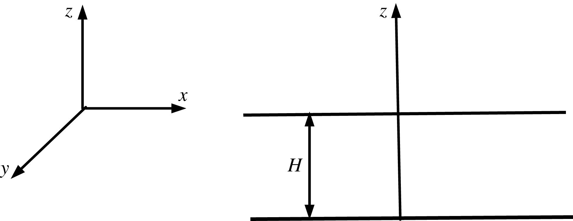
Schematic representation of the stably stratified fluid.

The conclusion contains a summary and a discussion of results. Some technical details of the calculations are given in appendices A and B.
2 Part I. Free wave BL in a stratified fluid
2.1 Statement of the problem and some general properties of the solution
We now consider a continuously stratified fluid confined between two parallel rigid lids
 $z=0,-H$
(figure 1). In the linear approximation the system is described by the equations:
 $$\begin{eqnarray}\boldsymbol{u}_{t}+\boldsymbol{e}_{z}b=-\unicode[STIX]{x1D735}p,\quad b_{t}-N^{2}w=0,\quad \unicode[STIX]{x1D735}\boldsymbol{\cdot }\boldsymbol{u}=0,\end{eqnarray}$$
with the no-flux boundary conditions and initial conditions:
 $$\begin{eqnarray}w|_{z=0,-H}=0;\quad (u,v,b)_{t=0}=(u_{I},v_{I},b_{I}).\end{eqnarray}$$
Here
 $\boldsymbol{u}=(u,v,w)$
is the velocity with components
 $u,v,w$
along the
 $x$
-,
 $y$
-,
 $z$
-axes, respectively;
 $b=g\unicode[STIX]{x1D70C}/\unicode[STIX]{x1D70C}_{0}$
is the buoyancy;
 $\unicode[STIX]{x1D70C}/\unicode[STIX]{x1D70C}_{0}$
,
 $p$
are the variations of density and pressure from their hydrostatic profiles divided by the reference density
 $\unicode[STIX]{x1D70C}_{0}$
;
 $N$
is the buoyancy frequency;
 $\boldsymbol{e}_{x},\boldsymbol{e}_{y},\boldsymbol{e}_{z}$
are the unit vectors along the axes
 $x,y,z$
, respectively; here and below the subscript ‘
 $I$
’ denotes initial values.
Let us discuss some general properties of solution to the problem (2.1), (2.2). The system (2.1) conserves the vertical component of vorticity:
 $$\begin{eqnarray}\unicode[STIX]{x1D6FA}^{z}=v_{x}-u_{y}=\unicode[STIX]{x1D6FA}_{I}^{z}=v_{Ix}-u_{Iy},\end{eqnarray}$$
and, in view of (2.1b
) and (2.2a,b
), the buoyancy at the boundaries
 $z=0,-H$
:
 $$\begin{eqnarray}b|_{z=0,-H}=b_{I}|_{z=0,-H}.\end{eqnarray}$$
The behaviour of
 $u,v,b$
at large times depends strongly on the buoyancy boundary fields
 $b_{I}|_{z=0,-H}$
. For example, assuming that all fields and their derivatives are bounded in time, we have from (2.1), (2.3) the following equations for the time means
 $\bar{u},\bar{v},\bar{w},\bar{p},\bar{b}$
:
 $$\begin{eqnarray}\bar{w}=\bar{p}_{x}=\bar{p}_{y}=0,\quad \bar{p}_{z}=-\bar{b},\quad \bar{u}_{x}+\bar{v}_{y}=0,\quad \bar{v}_{x}-\bar{u}_{y}=v_{Ix}-u_{Iy},\end{eqnarray}$$
where
 $$\begin{eqnarray}\bar{a}=\lim _{T_{0}\rightarrow \infty }\frac{1}{T_{0}}\int _{0}^{T_{0}}a\,\text{d}t.\end{eqnarray}$$
It follows from (2.5a,b
) that
 $\unicode[STIX]{x1D6FB}_{2}\bar{b}=0$
(
 $\unicode[STIX]{x1D6FB}_{2}=\boldsymbol{e}_{x}\unicode[STIX]{x2202}_{x}+\boldsymbol{e}_{y}\unicode[STIX]{x2202}_{y}$
) therefore in the case
 $$\begin{eqnarray}\unicode[STIX]{x1D6FB}_{2}b_{I}|_{z=0,-H}\neq 0\end{eqnarray}$$
the boundary condition (2.4) for the buoyancy does not agree with (2.5a,b ).
Similar discrepancies also occur for the horizontal velocities. Under the condition (2.7) the vertical gradients of horizontal velocities grow linearly in time in the vicinity of the boundaries since it follows from (2.1a ) and (2.4) that
 $$\begin{eqnarray}(u_{z},v_{z})_{z=0,-H}=t\unicode[STIX]{x1D6FB}_{2}(b_{I})_{z=0,-H}+(u_{Iz},v_{Iz})_{z=0,-H}.\end{eqnarray}$$
By virtue of (2.8)
 $(\bar{u}_{z},\bar{v}_{z})_{z=0,-H}=\infty$
, that, obviously, does not agree with equations (2.5c,d
) which determine
 $\bar{u},\bar{v}$
in a unique way given the initial fields
 $u_{I},v_{I}$
.
These peculiarities indicate that at large
 $t$
the fields
 $u,v,b$
have a boundary layer structure near the boundaries when, for example, the buoyancy
 $b$
near
 $z=0$
is represented as:
 $$\begin{eqnarray}b=b(x,y,zt),\end{eqnarray}$$
where the right-hand side tends to zero for any
 $z<0$
,
 $t\rightarrow \infty$
but
 $b(x,y,0)\neq 0$
. The boundary layer will be considered in § 2.3; in § 2.2 we derive the solution to (2.1), (2.2) in the form of expansions in vertical wave modes.
2.2 Expansions in vertical wave modes
In this subsection we obtain an exact solution to the problem (2.1), (2.2) in the form of expansions in vertical wave modes. For simplicity, the buoyancy frequency
 $N$
is assumed to be constant. First we consider the vertical velocity
 $w$
. Using the length and time scales
 $H$
and
 $1/N$
, the non-dimensional problem for
 $w$
(see, e.g. Miropol’sky Reference Miropol’sky2001) is reduced to the equation
 $$\begin{eqnarray}\unicode[STIX]{x1D6FB}^{2}w_{tt}+\unicode[STIX]{x1D6FB}_{2}^{2}w=0,\end{eqnarray}$$
with the no-flux condition (2.2a ) and initial conditions
 $$\begin{eqnarray}(w,w_{t})_{t=0}=(w_{I},{\dot{w}}_{I}),\quad w_{I}=-\int _{-1}^{z}(\unicode[STIX]{x2202}_{x}u_{I}+\unicode[STIX]{x2202}_{y}v_{I})\,\text{d}z.\end{eqnarray}$$
The initial field
 ${\dot{w}}_{I}$
in (2.11a
) can be expressed in terms of
 $b_{I}$
(see appendix A).
The solution to (2.10), (2.11) is written as the Fourier integral in the horizontal coordinates,
 $$\begin{eqnarray}w=\int {\hat{w}}(\unicode[STIX]{x1D73F},z,t)\text{e}^{\text{i}(kx+ly)}\text{d}\unicode[STIX]{x1D73F},\quad \unicode[STIX]{x1D73F}=(k,l),\end{eqnarray}$$
and for the Fourier amplitude
 ${\hat{w}}$
we have:
 $$\begin{eqnarray}({\hat{w}}_{zz}-\unicode[STIX]{x1D705}^{2}{\hat{w}})_{tt}-\unicode[STIX]{x1D705}^{2}{\hat{w}}=0,\quad {\hat{w}}|_{z=0,-1}=0,\quad ({\hat{w}},{\hat{w}}_{t})_{t=0}=({\hat{w}}_{I},\hat{{\dot{w}}}_{I}).\end{eqnarray}$$
Here and below the hat denotes the corresponding Fourier amplitude. The solution
 ${\hat{w}}$
is represented as the expansion in vertical wave modes:
 $$\begin{eqnarray}{\hat{w}}=\mathop{\sum }_{n=1}^{\infty }[{\hat{w}}_{In}\cos (\unicode[STIX]{x1D70E}_{n}t)+(\hat{{\dot{w}}}_{In}/\unicode[STIX]{x1D70E}_{n})\sin (\unicode[STIX]{x1D70E}_{n}t)]\sin n\unicode[STIX]{x03C0}z,\end{eqnarray}$$
where
 ${\hat{w}}_{In},\hat{{\dot{w}}}_{In}$
are the coefficients in analogous expansions for
 ${\hat{w}}_{I},\hat{{\dot{w}}}_{I}$
,
 $$\begin{eqnarray}({\hat{w}}_{In},\hat{{\dot{w}}}_{In})=2\int _{-1}^{0}({\hat{w}}_{I},\hat{{\dot{w}}}_{I})\sin n\unicode[STIX]{x03C0}z\,\text{d}z,\end{eqnarray}$$
 $\unicode[STIX]{x1D70E}_{n}=\unicode[STIX]{x1D705}/\sqrt{\unicode[STIX]{x1D705}^{2}+n^{2}\unicode[STIX]{x03C0}^{2}}$
is the frequency of the
 $n$
th vertical mode.
Knowing
 ${\hat{w}}$
we can find the Fourier amplitudes
 $\hat{u} ,\hat{v}$
of the horizontal velocities:
 $$\begin{eqnarray}(\hat{u} ,\hat{v})=(\hat{\bar{u}},\hat{\bar{v}})+(\hat{\tilde{u} },\hat{\tilde{v}}),\quad (\hat{\tilde{u} },\hat{\tilde{v}})=\text{i}(k,l){\hat{w}}_{z}/\unicode[STIX]{x1D705}^{2};\end{eqnarray}$$
here
 $(\hat{\bar{u}},\hat{\bar{v}})$
are the Fourier amplitudes of the stationary components
 $(\bar{u},\bar{v})$
determined from (2.5c,d
). Differentiation of (2.14) with respect to
 $z$
gives:
 $$\begin{eqnarray}{\hat{w}}_{z}=\unicode[STIX]{x03C0}\mathop{\sum }_{n=1}^{\infty }n[{\hat{w}}_{In}\cos (\unicode[STIX]{x1D70E}_{n}t)+(\hat{{\dot{w}}}_{In}/\unicode[STIX]{x1D70E}_{n})\sin (\unicode[STIX]{x1D70E}_{n}t)]\cos n\unicode[STIX]{x03C0}z.\end{eqnarray}$$
The problem for the buoyancy is very similar to that for
 $w$
:
 $$\begin{eqnarray}\unicode[STIX]{x1D6FB}^{2}b_{tt}+\unicode[STIX]{x1D6FB}_{2}^{2}b=0,\quad b|_{z=0,-1}=b_{I}|_{z=0,-1},\quad (b,b_{t})_{t=0}=(b_{I},w_{I}).\end{eqnarray}$$
The solution to (2.18) in terms of the Fourier amplitude
 $\hat{b}$
has the form (cf. (2.14)):
 $$\begin{eqnarray}\displaystyle & \displaystyle \hat{b}=\hat{b}_{I}+\mathop{\sum }_{n=1}^{\infty }\{\hat{b}_{In}[\cos (\unicode[STIX]{x1D70E}_{n}t)-1]+({\hat{w}}_{In}/\unicode[STIX]{x1D70E}_{n})\sin (\unicode[STIX]{x1D70E}_{n}t)\}\sin n\unicode[STIX]{x03C0}z, & \displaystyle\end{eqnarray}$$
 $$\begin{eqnarray}\displaystyle & \displaystyle \hat{b}_{In}=2\int _{-1}^{0}\hat{b}_{I}\sin n\unicode[STIX]{x03C0}z\,\text{d}z. & \displaystyle\end{eqnarray}$$
The formulae (2.14), (2.15), (2.16), (2.17) and (2.19) represent the exact solution in the form of expansions in vertical wave modes.
Let us compare the expansion (2.14) for
 ${\hat{w}}$
with the expansion (2.19) for
 $\hat{b}$
. Convergence of the expansions each depends on the asymptotic behaviour of the
 $n$
th term of the expansion for
 $n\rightarrow \infty$
. By virtue of the conditions
 $(w_{I},{\dot{w}}_{I})_{z=0,-1}=0$
the coefficients
 ${\hat{w}}_{In},\hat{{\dot{w}}}_{In}$
decay rapidly with increasing
 $n$
:
 $$\begin{eqnarray}{\hat{w}}_{In}=O(n^{-3}),\quad \hat{{\dot{w}}}_{In}=O(n^{-3}),\quad n\rightarrow \infty .\end{eqnarray}$$
Since
 $\unicode[STIX]{x1D70E}_{n}=O(n^{-1}),n\rightarrow \infty$
, the
 $n$
th term in (2.14) is
 $O(n^{-2})$
, independent of
 $t$
, and the series (2.14) converges absolutely and uniformly in the domain
 $[-1\leqslant z\leqslant 0]\times [0\leqslant t\leqslant \infty ]$
. Therefore the vertical velocity
 $w$
is a smooth function of
 $z$
at any time
 $t$
(see the numerical example below in this subsection).
The behaviour of the expansion (2.19) for the buoyancy is somewhat different. If
 $b_{I}|_{z=0,-1}=0$
then
 $\hat{b}_{In}=O(n^{-3}),n\rightarrow \infty$
, and the buoyancy, like
 $w$
, is a smooth function of
 $z$
at any time
 $t$
. However, in the case (2.7) we have
 $$\begin{eqnarray}\hat{b}_{In}=O(n^{-1}),\quad n\rightarrow \infty ,\end{eqnarray}$$
and the
 $n$
th term in (2.19a
) is
 $O(n^{-3}),n\rightarrow \infty$
for any finite fixed
 $t$
. At the same time, this estimate is not uniform in
 $t$
since
 $\unicode[STIX]{x1D70E}_{n}t\sim t/n$
for large
 $n$
, therefore the series (2.19a
) converges absolutely and uniformly in the domain
 $[-1\leqslant z\leqslant 0]\times [0\leqslant t\leqslant t_{0}]$
for any finite fixed
 $t_{0}$
, but, generally, not in the domain
 $[-1\leqslant z\leqslant 0]\times [0\leqslant t\leqslant \infty ]$
. A similar situation takes place for the horizontal velocities
 $\hat{\tilde{u} },\hat{\tilde{v}}$
since in (2.17)
 $n\hat{{\dot{w}}}_{In}/\unicode[STIX]{x1D70E}_{n}=O(n^{-1})$
,
 $n\rightarrow \infty$
. One can say, therefore, that at large
 $t$
the expansions (2.17) and (2.19) for the horizontal velocities and buoyancy converge worse than the expansion (2.14) for
 $w$
.
The ‘bad’ convergence of the series (2.17), (2.19a
) results in non-stationary BLs in the fields of horizontal velocity and buoyancy at large times. Any partial sum in the series (2.17), (2.19a
) has no ‘boundary layer’ form (2.9) and the time mean (2.6) of the sum is always zero. This means that such a BL is a result of the joint impact of the low-frequency wave harmonics with numbers
 $1\ll n\leqslant \infty$
in the series (2.17), (2.19a
). That is why the non-stationary BL will be called the wave boundary layer.
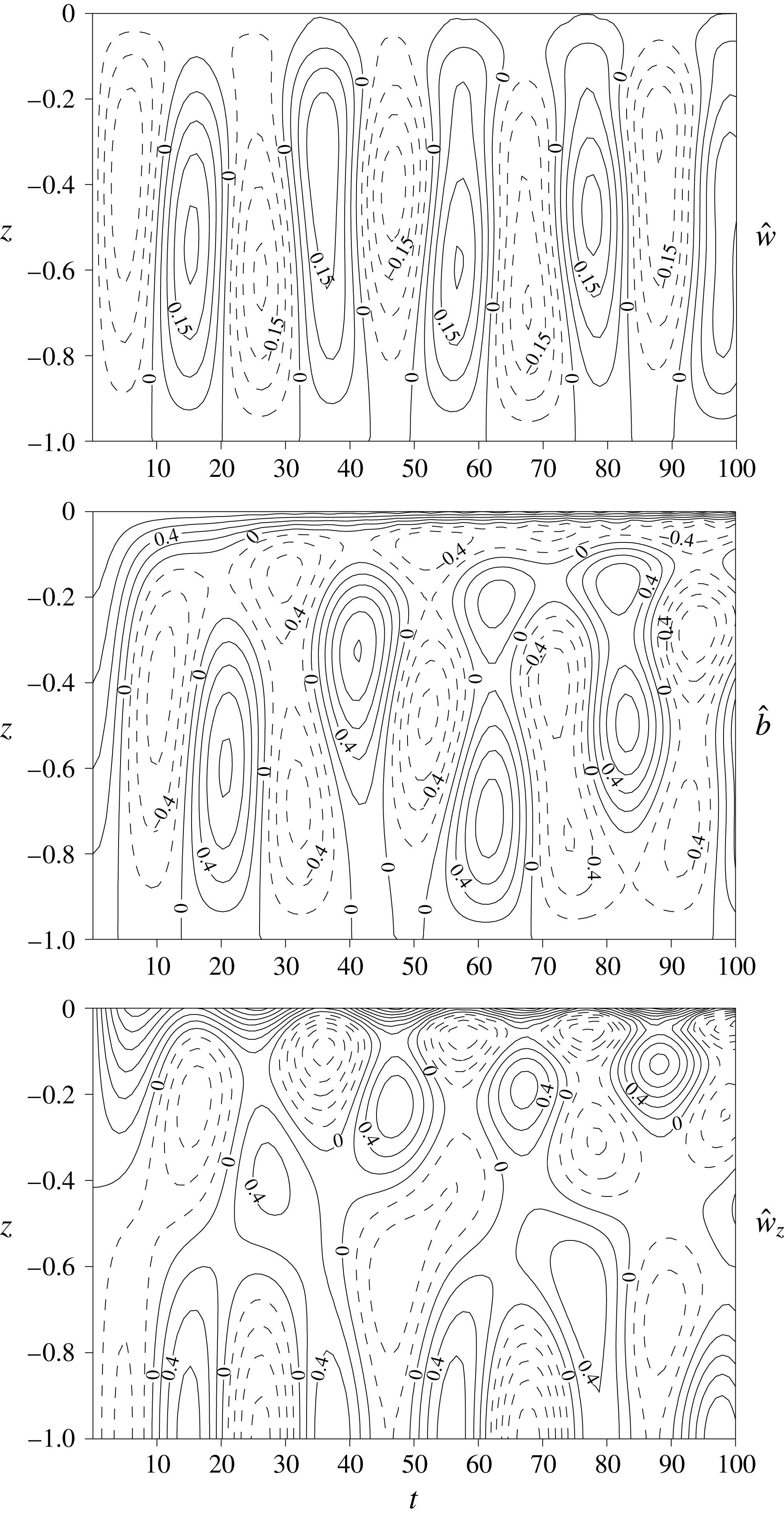
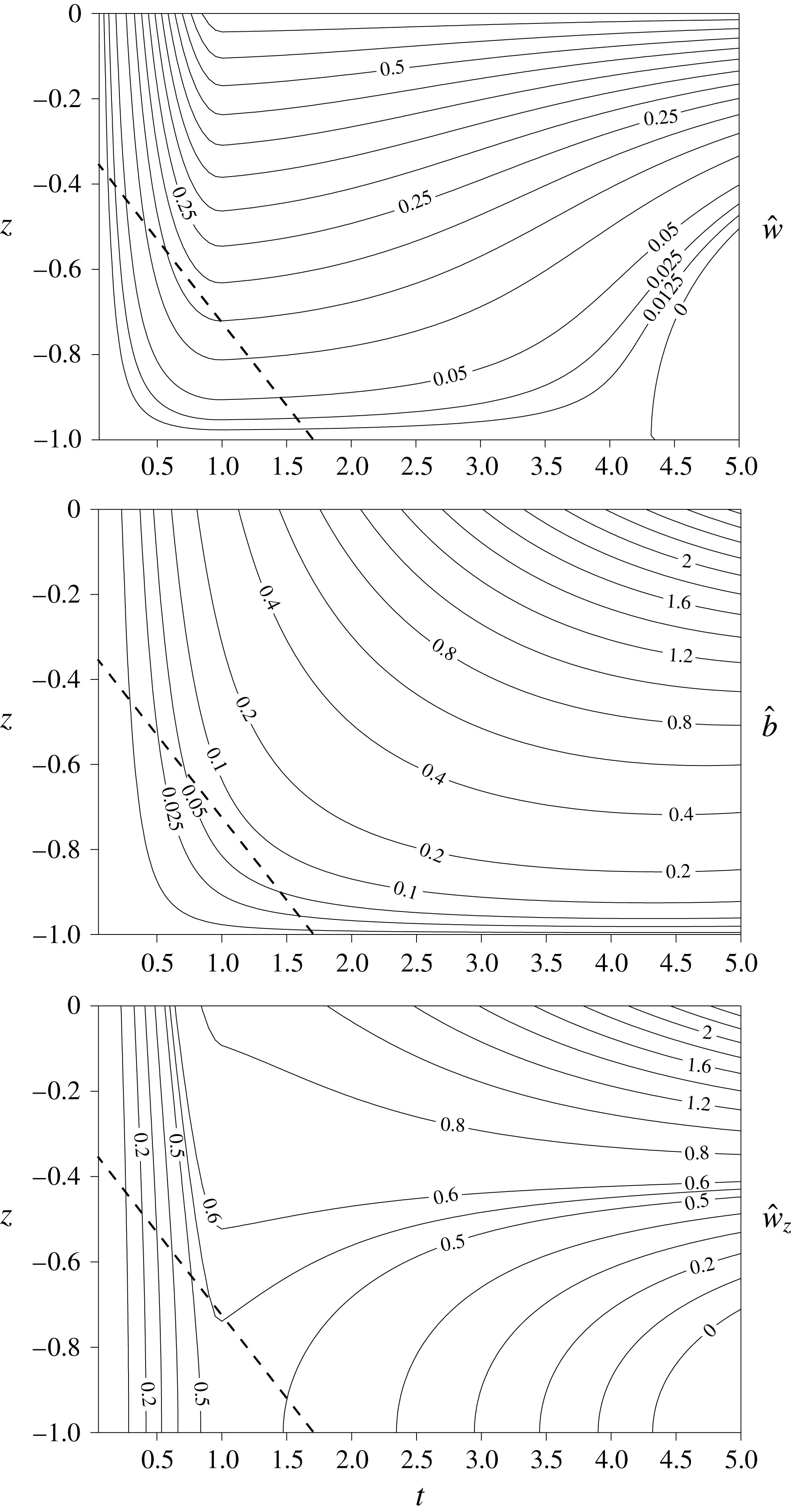
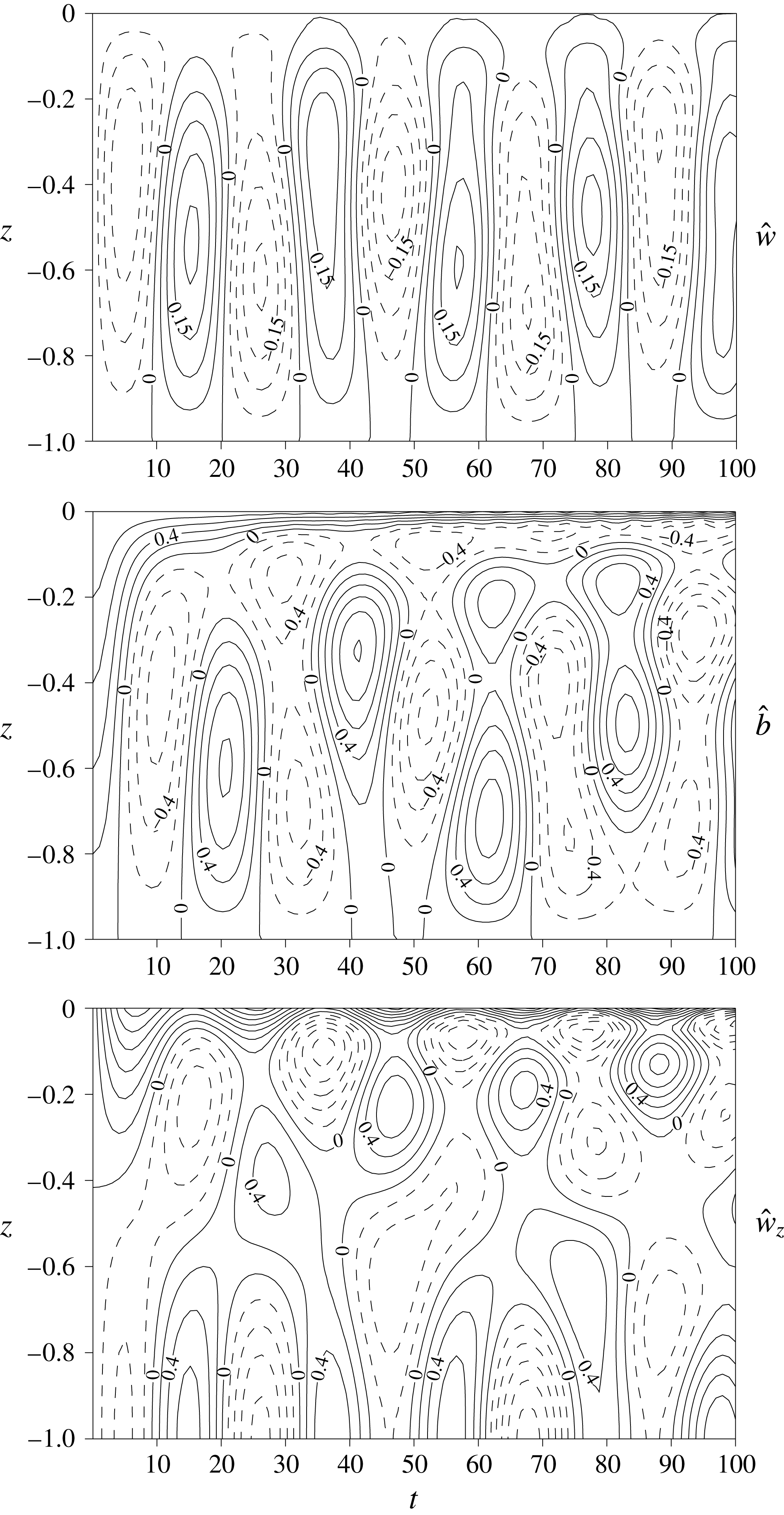
Isolines of the functions
 ${\hat{w}}(z,t),\hat{b}(z,t),{\hat{w}}_{z}(z,t)$
; contour intervals in the fields
 ${\hat{w}},\hat{b},{\hat{w}}_{z}$
are 0.05, 0.2, 0.2 respectively. The dashed isolines are negative.
To illustrate development of the BL we consider the solution to (2.1), (2.2) corresponding to the initial condition
 $$\begin{eqnarray}u_{I}=v_{I}=0,b_{I}=\exp [\text{i}(kx+ly)](z+1).\end{eqnarray}$$
In this case
 $w_{I}=0$
and the buoyancy vanishes at the bottom
 $z=-1$
, therefore the BL exists only near the surface
 $z=0$
. The solutions for
 $w,b$
are sought in the form:
 $$\begin{eqnarray}w={\hat{w}}(z,t)\exp [\text{i}(kx+ly)],\quad b=\hat{b}(z,t)\exp [\text{i}(kx+ly)],\end{eqnarray}$$
and the corresponding expansions for
 ${\hat{w}},\hat{b},{\hat{w}}_{z}$
can be found in appendix A. Isolines of the functions
 ${\hat{w}}(z,t),\hat{b}(z,t),{\hat{w}}_{z}(z,t)$
are shown in figure 2. The BL is absent in the vertical velocity field
 ${\hat{w}}$
which oscillates almost periodically in time at any
 $z=\text{const.}$
with a frequency near to the frequency of the first baroclinic mode
 $\unicode[STIX]{x1D70E}_{1}=\unicode[STIX]{x1D705}/\sqrt{\unicode[STIX]{x1D705}^{2}+\unicode[STIX]{x03C0}^{2}}$
(
 $\unicode[STIX]{x1D70E}_{1}\cong 0.3$
for
 $\unicode[STIX]{x1D705}=1$
). In the buoyancy field
 $\hat{b}$
the BL is the narrow domain near the surface
 $z=0$
characterized by sharp vertical gradients of
 $\hat{b}$
; the domain thickness decreases and the gradients increase with increasing time. An analogous boundary layer develops in the field of the derivative
 ${\hat{w}}_{z}$
; its thickness oscillates in time unlike the BL in the buoyancy. Below the BLs the fields
 $\hat{b},{\hat{w}}_{z}$
oscillate in time like the vertical velocity
 ${\hat{w}}$
. In the next section we obtain asymptotic solutions for the BL fields.
2.3 Wave boundary layer
The expansions (2.14), (2.17) and (2.19a
) are poorly suited to describing boundary layer structures which rapidly change in space with the scale decreasing with increasing time: the vertical scale of
 $n$
th partial sum of the series cannot be smaller than
 $H/n$
for all times. To construct an asymptotic BL solution valid on large times we apply the method used in Il’in (Reference Il’in1970, Reference Il’in1972), Kamenkovich & Kamenkovich (Reference Kamenkovich and Kamenkovich1993) to study Rossby waves in a bounded basin. We consider the problem (2.18) for the buoyancy and introduce a new variable
 $B$
– the buoyancy averaged over the time interval
 $[0,t]$
for each
 $t$
(cf. Il’in Reference Il’in1970, Reference Il’in1972; Kamenkovich & Kamenkovich Reference Kamenkovich and Kamenkovich1993):
 $$\begin{eqnarray}B=\frac{1}{t}\int _{0}^{t}b\,\text{d}t,\quad b=(tB)_{t}.\end{eqnarray}$$
The meaning of the variable
 $B$
is that the contribution of the rapidly oscillating part of the field
 $b$
to
 $B$
becomes negligible at large times
 $t\gg 1$
, as seen from (2.19a
). In what follows
 $b$
and
 $B$
will be referred to as the instantaneous and averaged field, respectively; similarly for other physical quantities. In terms of
 $B$
the problem (2.18a,b
) takes the form:
 $$\begin{eqnarray}\unicode[STIX]{x1D6FB}^{2}B_{tt}+\frac{2}{t}\unicode[STIX]{x1D6FB}^{2}B_{t}+\unicode[STIX]{x1D6FB}_{2}^{2}B=\frac{1}{t}\unicode[STIX]{x1D6FB}^{2}w_{I},\quad B|_{z=0,-1}=b_{I}|_{z=0,-1}.\end{eqnarray}$$
Let us consider the solution to (2.25) at large times. Far from the boundaries the vertical scale is assumed to be of the order of the layer depth and the solution here is sought in the following asymptotic form:
 $$\begin{eqnarray}B=\frac{1}{t}B_{1}(x,y,z)+\frac{1}{t^{2}}B_{2}(x,y,z)+\cdots \,.\end{eqnarray}$$
Substitution of (2.26) into (2.25a ) gives:
 $$\begin{eqnarray}\unicode[STIX]{x1D6FB}_{2}^{2}B_{1}=\unicode[STIX]{x1D6FB}^{2}w_{I}.\end{eqnarray}$$
Generally, the lowest-order inner solution
 $B_{1}/t$
does not satisfy the boundary conditions (2.25b
); this discrepancy is corrected by boundary layers confined to narrow regions near the boundaries. The solution near
 $z=0$
is sought in the form of the following expansion:
 $$\begin{eqnarray}B=D_{0}(x,y,\unicode[STIX]{x1D709})+\frac{1}{t}D_{1}(x,y,\unicode[STIX]{x1D709})+\cdots \,,\quad \unicode[STIX]{x1D709}=-zt,\end{eqnarray}$$
where
 $\unicode[STIX]{x1D709}$
is the ‘stretched’ coordinate in the boundary layer.
At the leading order we have the equation:
 $$\begin{eqnarray}\unicode[STIX]{x1D709}^{2}D_{0}^{(4)}+6\unicode[STIX]{x1D709}D_{0}^{(3)}+6D_{0}^{\prime \prime }+\unicode[STIX]{x1D6FB}_{2}^{2}D_{0}=0,\end{eqnarray}$$
where the superscripts and primes mean differentiation with respect to
 $\unicode[STIX]{x1D709}$
. The function
 $D_{0}$
satisfies the boundary conditions:
 $$\begin{eqnarray}D_{0}|_{\unicode[STIX]{x1D709}=0}=b_{I}|_{z=0};\quad D_{0}\rightarrow 0,\quad \unicode[STIX]{x1D709}\rightarrow \infty .\end{eqnarray}$$
The corresponding equations for the Fourier amplitude
 $\hat{D}_{0}$
have the form:
 $$\begin{eqnarray}\unicode[STIX]{x1D709}^{2}\hat{D}_{0}^{(4)}+6\unicode[STIX]{x1D709}\hat{D}_{0}^{(3)}+6\hat{D^{\prime \prime }}_{0}-\unicode[STIX]{x1D705}^{2}\hat{D}_{0}=0;\quad \hat{D}_{0}|_{\unicode[STIX]{x1D709}=0}=\hat{b}_{I}|_{z=0};\quad \hat{D}_{0}\rightarrow 0,\unicode[STIX]{x1D709}\rightarrow \infty .\end{eqnarray}$$
The regular solution to (2.31) can be written as (Kamke Reference Kamke1976):
 $$\begin{eqnarray}\hat{D}_{0}=\frac{\hat{b}_{I}|_{z=0}}{\sqrt{\unicode[STIX]{x1D705}\unicode[STIX]{x1D709}}}\text{J}_{1}(2\sqrt{\unicode[STIX]{x1D705}\unicode[STIX]{x1D709}}),\end{eqnarray}$$
where here and below
 $\text{J}_{n}$
is the Bessel function of the
 $n$
th order. Thus at large times the averaged buoyancy is equal to
 $$\begin{eqnarray}\hat{B}=\frac{\hat{b}_{I}|_{z=0}}{\sqrt{\unicode[STIX]{x1D705}\unicode[STIX]{x1D709}}}\text{J}_{1}(2\sqrt{\unicode[STIX]{x1D705}\unicode[STIX]{x1D709}})+O(1/t).\end{eqnarray}$$
Non-stationary components of the horizontal velocities are determined by the vertical derivative
 $w_{z}$
(see (2.16b
). It follows from (2.1b
) and (2.24) that
 $$\begin{eqnarray}W_{z}=\frac{1}{t}\int _{0}^{t}w_{z}\,\text{d}t=B_{zt}+\frac{1}{t}B_{z}-\frac{b_{Iz}}{t};\end{eqnarray}$$
using (2.33) one finds the Fourier amplitude of
 $W_{z}$
:
 $$\begin{eqnarray}{\hat{W}}_{z}=\frac{\unicode[STIX]{x1D705}\hat{b}_{I}|_{z=0}}{\sqrt{\unicode[STIX]{x1D705}\unicode[STIX]{x1D709}}}\text{J}_{1}(2\sqrt{\unicode[STIX]{x1D705}\unicode[STIX]{x1D709}})-\frac{\hat{b}_{Iz}}{t}.\end{eqnarray}$$
In (2.33), (2.35) the stretched coordinate
 $\unicode[STIX]{x1D709}$
is multiplied by the non-dimensional horizontal wavenumber
 $\unicode[STIX]{x1D705}$
, therefore boundary layers for different Fourier harmonics in (2.12) differ from each other. With increasing
 $\unicode[STIX]{x1D705}$
(i.e. for shorter harmonics), the corresponding BL develops faster and the vertical gradients in it become sharper. The near-bottom BL can be treated in the same way.
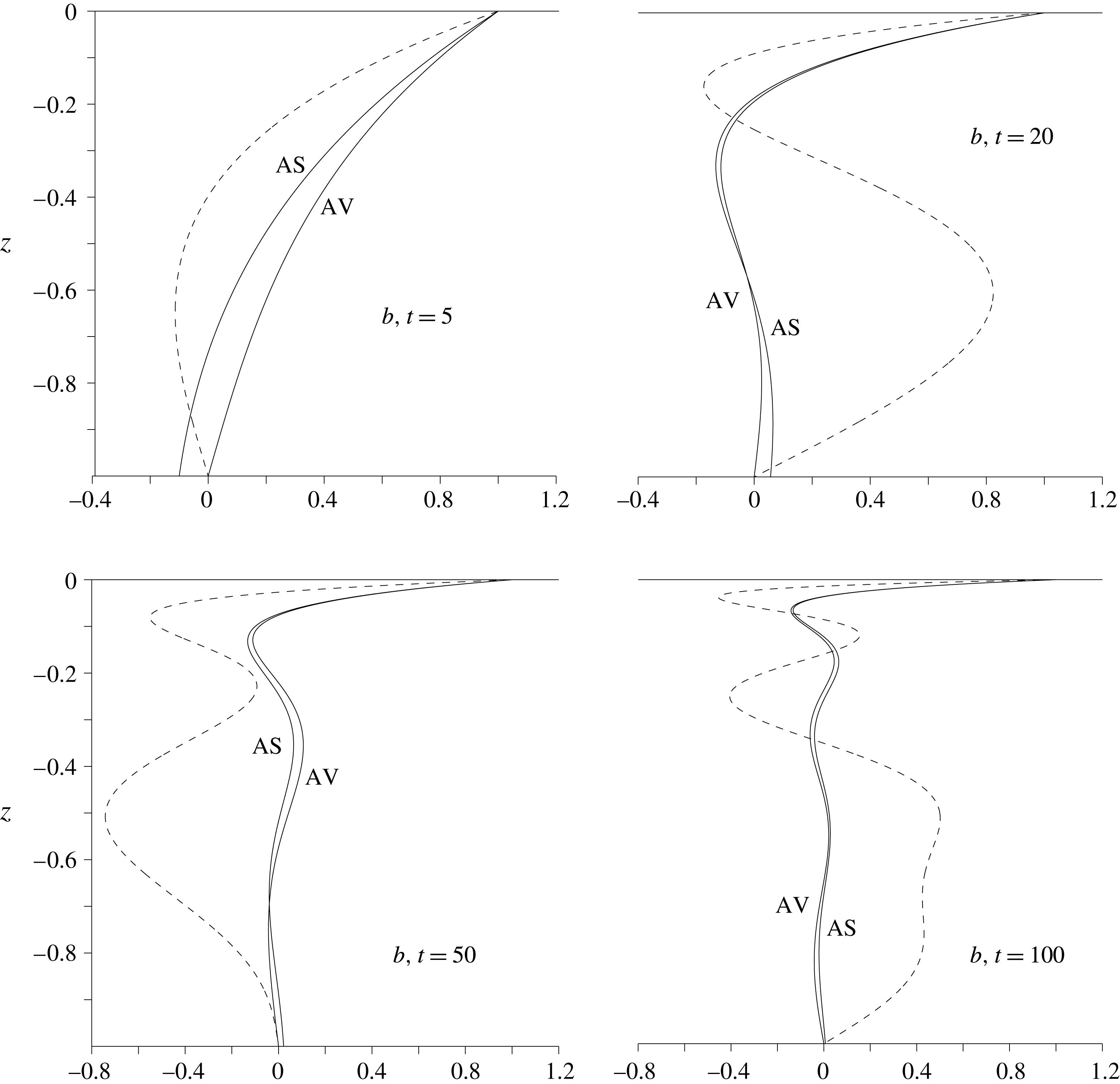
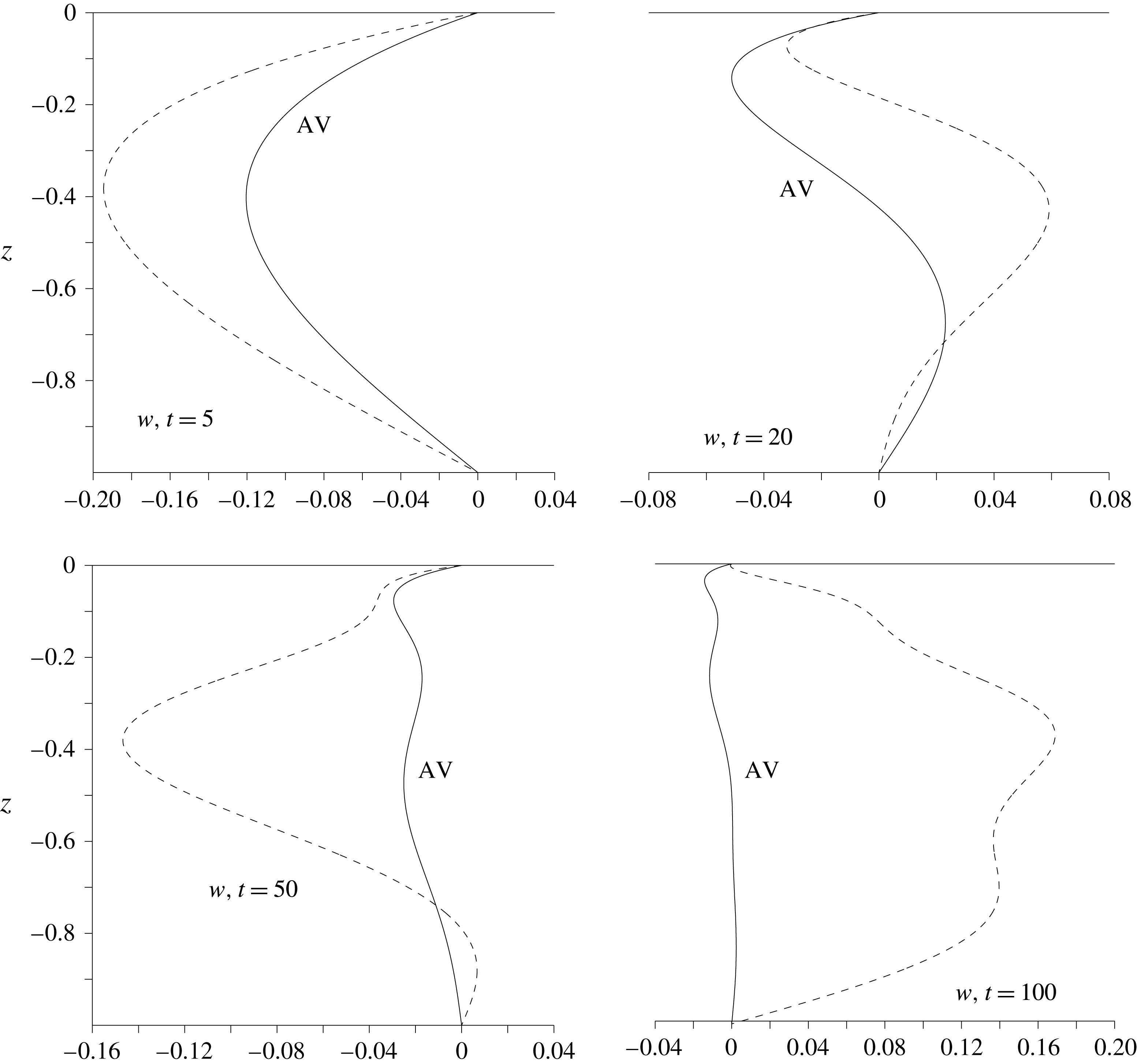
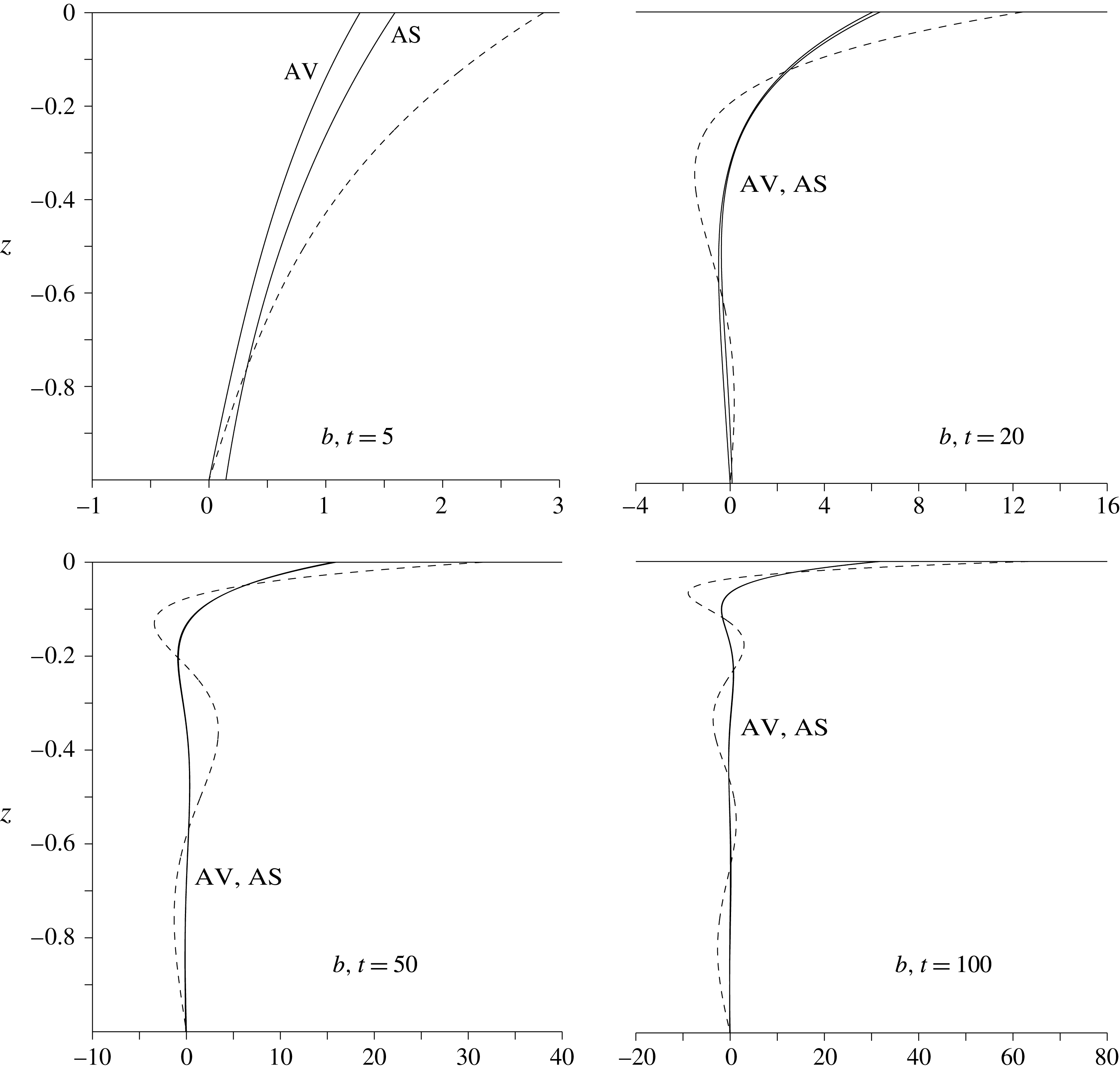
Vertical profiles of the Fourier amplitude of the buoyancy
 $b$
at different times. The instantaneous profiles of
 $\hat{b}$
are given by the dashed lines, the solid lines represent the asymptotic (AS) and exact (AV) profiles of the averaged fields
 $\hat{B}$
;
 $N=\text{const.}$
,
 $\unicode[STIX]{x1D705}=1$
.

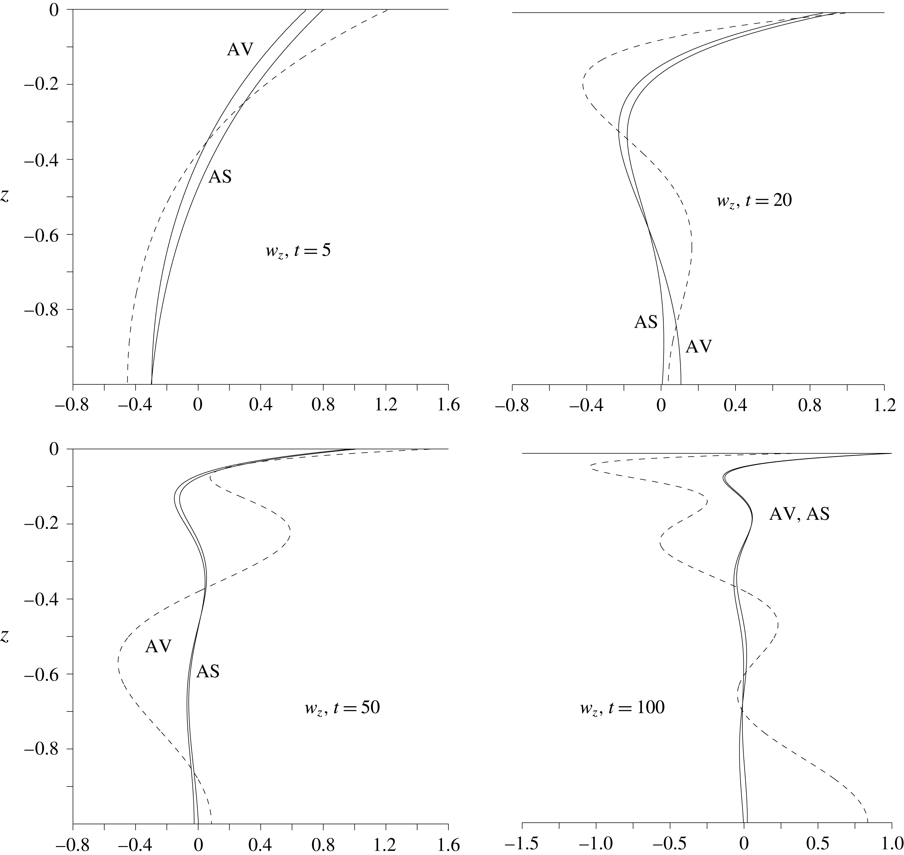
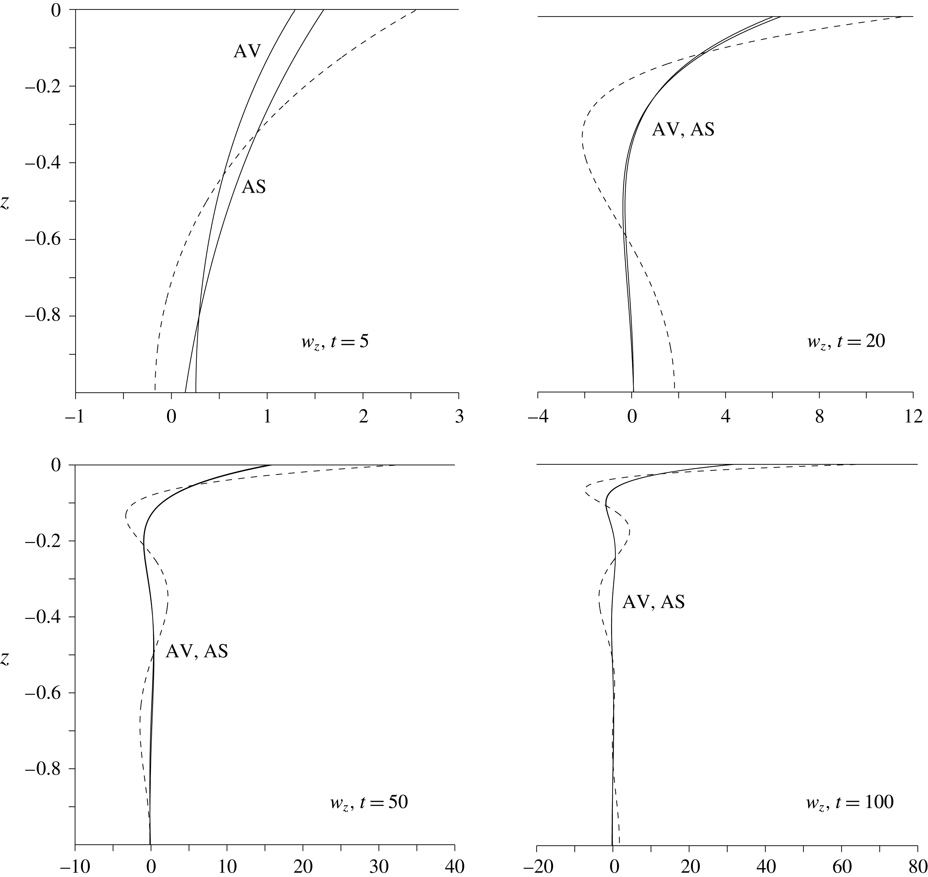
The same as in figure 3 but for the derivative
 $w_{z}$
.

The same as in figure 3 but for the vertical velocity
 $w$
.

Exact fields
 $\hat{B}$
and
 ${\hat{W}}_{z}$
can be found from (2.14), (2.19a
):
 $$\begin{eqnarray}\displaystyle & \displaystyle \hat{B}=\hat{b}_{I}+\mathop{\sum }_{n=1}^{\infty }\left\{\hat{b}_{In}\left[\frac{\sin (\unicode[STIX]{x1D70E}_{n}t)}{\unicode[STIX]{x1D70E}_{n}t}-1\right]+{\hat{w}}_{In}\frac{1-\cos (\unicode[STIX]{x1D70E}_{n}t)}{\unicode[STIX]{x1D70E}_{n}^{2}t}\right\}\sin n\unicode[STIX]{x03C0}z, & \displaystyle\end{eqnarray}$$
 $$\begin{eqnarray}\displaystyle & \displaystyle {\hat{W}}_{z}=\unicode[STIX]{x03C0}\mathop{\sum }_{n=1}^{\infty }n\left[{\hat{w}}_{In}\frac{\sin (\unicode[STIX]{x1D70E}_{n}t)}{\unicode[STIX]{x1D70E}_{n}t}+\hat{{\dot{w}}}_{In}\frac{1-\cos (\unicode[STIX]{x1D70E}_{n}t)}{\unicode[STIX]{x1D70E}_{n}^{2}t}\right]\cos n\unicode[STIX]{x03C0}z. & \displaystyle\end{eqnarray}$$
So, we have the exact solutions (2.36) and approximate asymptotic solutions (2.33) and (2.35). In the next section we numerically compare the exact and asymptotic solutions for the initial conditions (2.22).
2.4 Comparison of asymptotic and exact solutions
To check validity of the asymptotics (2.33), (2.35) and to estimate how rapidly the asymptotic regime is reached (if at all), we performed numerical experiments with the solution obeying the initial conditions (2.22). The corresponding averaged fields
 $\hat{B},{\hat{W}}_{z}$
are given in appendix A. To compare the fields with their asymptotic representations (2.33), (2.35) and the instantaneous fields
 $\hat{b},{\hat{w}},{\hat{w}}_{z}$
, we calculated numerically the obtained solutions at different times. Examples of the calculations are shown in figures 3–5.
One can see that the instantaneous profiles differ strongly from the profiles of the averaged fields. At the same time, the asymptotics (2.33), (2.35) describe the exact fields (2.36) fairly well even at
 $t=5$
, and are very close to them after
 $t=20$
. The time-averaged fields actually have a boundary layer structure, becoming more and more concentrated near the upper boundary and tending to zero in the inner domain with increasing time, in line with the asymptotic solution. The process is accompanied by a strong increase of vertical gradients of the buoyancy (figure 3) and horizontal velocity (
 $\hat{u} ,\hat{v}\sim {\hat{w}}_{z}$
, figure 4) near the surface
 $z=0$
. The instantaneous profiles do not decay anywhere with increasing time and oscillate in time below the BL domain, the maximal vertical gradients (more sharp than in the time-averaged fields) developing near the upper boundary. For comparison the instantaneous and time-averaged vertical velocity profiles are shown in figure 5; in these profiles elements of boundary layer structure are absent (cf. figure 2).
3 Part II. Forced wave BL in a stratified fluid
In part I the motion was assumed to be unforced and non-viscous, but one can expect that the viscosity and forcing can have a pronounced effect on the BL evolution. In part II we examine dynamics of the wave BL in a viscous stratified fluid driven by tangential stresses exerted on the fluid surface.
3.1 Governing equations
For simplicity we take into account only the vertical diffusion of the horizontal momentum, choose the no-slip conditions on the fluid bottom and assume that
 $N=N_{0}=\text{const}$
. In this case the governing equations take the following form:
 $$\begin{eqnarray}u_{t}+p_{x}-\unicode[STIX]{x1D707}u_{zz}=0,\quad v_{t}+p_{y}-\unicode[STIX]{x1D707}v_{zz}=0,\quad w_{t}+b=-p_{z},\end{eqnarray}$$
 $$\begin{eqnarray}b_{t}-N_{0}^{2}w=0,\quad u_{x}+v_{y}+w_{z}=0.\end{eqnarray}$$
The boundary and initial conditions are written as follows:
 $$\begin{eqnarray}w|_{z=0,-H}=0,\quad \unicode[STIX]{x1D707}(u_{z},v_{z})_{z=0}=(\unicode[STIX]{x1D70F}_{x},\unicode[STIX]{x1D70F}_{y}),\quad (u_{z},v_{z})_{z=-H}=0,\end{eqnarray}$$
 $$\begin{eqnarray}u_{I}=v_{I}=b_{I}=0.\end{eqnarray}$$
Here
 $\unicode[STIX]{x1D707}$
is the kinematic viscosity,
 $\unicode[STIX]{x1D749}=(\unicode[STIX]{x1D70F}_{x},\unicode[STIX]{x1D70F}_{y})$
is the vector of surface stress.
We now introduce the scales of time
 $T_{s}$
, length
 $L_{s}$
, velocity
 $U_{s}$
, pressure
 $P_{s}$
and buoyancy
 $B_{s}$
:
 $$\begin{eqnarray}T_{s}=N_{0}^{-1},\quad L_{s}=H,\quad U_{s}=\unicode[STIX]{x1D70F}/\sqrt{\unicode[STIX]{x1D707}N_{0}},\quad P_{s}=U_{s}HN_{0},\quad B_{s}=U_{s}N_{0},\end{eqnarray}$$
and write (3.1), (3.2) in the non-dimensional form:
 $$\begin{eqnarray}u_{t}+p_{x}-\unicode[STIX]{x1D700}^{2}u_{zz}=0,\quad v_{t}+p_{y}-\unicode[STIX]{x1D700}^{2}v_{zz}=0,\quad w_{t}+b=-p_{z},\end{eqnarray}$$
 $$\begin{eqnarray}b_{t}-w=0,\quad u_{x}+v_{y}+w_{z}=0;\end{eqnarray}$$
 $$\begin{eqnarray}w|_{z=0,-1}=0,\quad \unicode[STIX]{x1D700}(u_{z},v_{z})_{z=0}=(\unicode[STIX]{x1D70F}_{x},\unicode[STIX]{x1D70F}_{y}),\quad (u_{z},v_{z})_{z=-1}=0,\end{eqnarray}$$
 $$\begin{eqnarray}u_{I}=v_{I}=b_{I}=0.\end{eqnarray}$$
Here
 $\unicode[STIX]{x1D700}$
is a small parameter,
 $$\begin{eqnarray}\unicode[STIX]{x1D700}=h_{B}/H\ll 1,\quad h_{B}=\sqrt{\unicode[STIX]{x1D707}/N_{0}};\end{eqnarray}$$
 $h_{B}$
is the typical depth of friction layer which is assumed to be much smaller than the fluid depth
 $H$
.
The smallness of
 $\unicode[STIX]{x1D700}$
allows us to seek for the solution as a sum of an inner solution and a solution for friction layer (FL) confined to a narrow domain near the fluid surface. The inner solution is smooth in
 $z$
and does not depend on friction at the lowest order. The FL solution depends on the stretched coordinate
 $\unicode[STIX]{x1D70D}=z/\unicode[STIX]{x1D700}$
in the boundary layer. Formally, the solution is sought in the following asymptotic form:
 $$\begin{eqnarray}\displaystyle & \displaystyle (u,v,w,p,b)=(u^{F},v^{F},w^{F},p^{F},b^{F})+(u^{in},v^{in},w^{in},p^{in},b^{in}), & \displaystyle\end{eqnarray}$$
 $$\begin{eqnarray}\displaystyle & \displaystyle (u^{F},v^{F})=(u_{0}^{F},v_{0}^{F})(x,y,\unicode[STIX]{x1D70D},t)+\unicode[STIX]{x1D700}(u_{1}^{F},v_{1}^{F})+\cdots \,, & \displaystyle\end{eqnarray}$$
 $$\begin{eqnarray}\displaystyle & \displaystyle (w^{F},b^{F})=\unicode[STIX]{x1D700}(w_{0}^{F},b_{0}^{F})(x,y,\unicode[STIX]{x1D70D},t)+\unicode[STIX]{x1D700}^{2}(w_{1}^{F},b_{1}^{F})+\cdots \,, & \displaystyle\end{eqnarray}$$
 $$\begin{eqnarray}\displaystyle & \displaystyle p^{F}=\unicode[STIX]{x1D700}^{2}p_{0}^{F}(x,y,\unicode[STIX]{x1D70D},t)+\unicode[STIX]{x1D700}^{3}p_{1}^{F}+\cdots \,, & \displaystyle\end{eqnarray}$$
 $$\begin{eqnarray}\displaystyle & \displaystyle (u^{in},v^{in},w^{in},p^{in},b^{in})=\unicode[STIX]{x1D700}(u_{0}^{in},v_{0}^{in},w_{0}^{in},p_{0}^{in},b_{0}^{in})+\unicode[STIX]{x1D700}^{2}(u_{1}^{in},v_{1}^{in},w_{1}^{in},p_{1}^{in},b_{1}^{in})+\cdots \,.\qquad & \displaystyle\end{eqnarray}$$
The superscripts ‘
 $F$
’ and ‘in’ denote the fields in friction layer and inner domains, respectively.
To the lowest order we have:
 $$\begin{eqnarray}u_{0t}^{F}-u_{0\unicode[STIX]{x1D70D}\unicode[STIX]{x1D70D}}^{F}=0,\quad v_{0t}^{F}-v_{0\unicode[STIX]{x1D70D}\unicode[STIX]{x1D70D}}^{F}=0,\quad w_{0t}^{F}+b_{0}^{F}=-p_{0\unicode[STIX]{x1D70D}}^{F},\end{eqnarray}$$
 $$\begin{eqnarray}b_{0t}^{F}-w_{0}^{F}=0,\quad u_{0x}^{F}+v_{0y}^{F}+w_{0\unicode[STIX]{x1D70D}}^{F}=0;\end{eqnarray}$$
 $$\begin{eqnarray}u_{0t}^{in}+p_{0x}^{in}=0,\quad v_{0t}^{in}+p_{0y}^{in}=0,\quad w_{0t}^{in}+b_{0}^{in}=-p_{0z}^{in},\end{eqnarray}$$
 $$\begin{eqnarray}b_{0t}^{in}-w_{0}^{in}=0,\quad u_{0x}^{in}+v_{0y}^{in}+w_{0z}^{in}=0.\end{eqnarray}$$
The initial conditions for all fields are zero and the boundary conditions take the form:
 $$\begin{eqnarray}(u_{0\unicode[STIX]{x1D70D}}^{F},v_{0\unicode[STIX]{x1D70D}}^{F})_{\unicode[STIX]{x1D70D}=0}=(\unicode[STIX]{x1D70F}_{x},\unicode[STIX]{x1D70F}_{y});\quad u_{0}^{F},v_{0}^{F}\rightarrow 0\quad \text{as }\unicode[STIX]{x1D70D}\rightarrow -\infty ;\end{eqnarray}$$
 $$\begin{eqnarray}(w_{0}^{F}+w_{0}^{in})_{z=0}=0,\quad w_{0}^{in}|_{z=-1}=0.\end{eqnarray}$$
We will be interested in the inner solution which can be determined without detailed calculation of the FL solution. Integrating (3.8a,b,e
) with respect to
 $\unicode[STIX]{x1D70D}$
from
 $-\infty$
to 0 and taking into account (3.10a,b
) we derive the equations:
 $$\begin{eqnarray}U_{0t}^{F}=\unicode[STIX]{x1D70F}_{x},\quad V_{0t}^{F}=\unicode[STIX]{x1D70F}_{y},\quad U_{0x}^{F}+V_{0y}^{F}+w_{0}^{F}|_{\unicode[STIX]{x1D70D}=0}=0,\end{eqnarray}$$
where
 $$\begin{eqnarray}(U_{0}^{F},V_{0}^{F})=\int _{-\infty }^{0}(u_{0}^{F},v_{0}^{F})\,\text{d}\unicode[STIX]{x1D70D}.\end{eqnarray}$$
It readily follows from (3.11) that:
 $$\begin{eqnarray}w_{0}^{F}|_{\unicode[STIX]{x1D70D}=0}=-\int _{0}^{t}\text{div}\unicode[STIX]{x1D749}\,\text{d}t,\end{eqnarray}$$
whence, taking into account (3.10c ), one obtains the boundary condition for the inner vertical velocity:
 $$\begin{eqnarray}w_{0}^{in}|_{z=0}=\int _{0}^{t}\text{div}\unicode[STIX]{x1D749}\,\text{d}t.\end{eqnarray}$$
We note that the condition (3.14) can be valid if the motion is turbulent and the viscous stresses
 $\unicode[STIX]{x1D707}u_{zz},\unicode[STIX]{x1D707}v_{zz}$
in (3.1a,b
) are replaced by the
 $z$
-derivatives of the momentum density fluxes
 $\unicode[STIX]{x2202}\unicode[STIX]{x1D70F}_{xz}/\unicode[STIX]{x2202}z,\unicode[STIX]{x2202}\unicode[STIX]{x1D70F}_{yz}/\unicode[STIX]{x2202}z$
, respectively. If the fluxes
 $\unicode[STIX]{x1D70F}_{xz},\unicode[STIX]{x1D70F}_{yz}$
are confined to a narrow turbulent layer near the surface
 $z=0$
and are negligibly small outside the layer, then the integration of (3.1a,b,e
) over the layer depth gives (3.14) as the boundary condition for domain under the turbulent layer.
3.2 Problem for the inner domain
In this section we obtain the inner solution in the form of expansions in vertical wave modes (cf. § 2.2) and discuss some properties of the solution. Equations (3.9), (3.10d
) and (3.14) are reduced to the following problem for
 $w_{0}^{in}$
(the subscript ‘0’ and superscript ‘in’ are omitted):
 $$\begin{eqnarray}\unicode[STIX]{x1D6FB}^{2}w_{tt}+\unicode[STIX]{x1D6FB}_{2}^{2}w=0,\quad w|_{z=0}=\int _{0}^{t}\text{div}\unicode[STIX]{x1D749}\,\text{d}t,\quad w|_{z=-1}=0,\quad w_{I}={\dot{w}}_{I}=0.\end{eqnarray}$$
We now represent
 $w$
as the sum
 $$\begin{eqnarray}w=F(x,y,t)(z+1)+w^{a},\quad F=\int _{0}^{t}\text{div}\unicode[STIX]{x1D749}\,\text{d}t,\end{eqnarray}$$
where
 $w^{a}$
obeys the equations:
 $$\begin{eqnarray}\unicode[STIX]{x1D6FB}^{2}w_{tt}^{a}+\unicode[STIX]{x1D6FB}_{2}^{2}w^{a}=-(z+1)\unicode[STIX]{x1D6FB}_{2}^{2}(F_{tt}+F),\quad w^{a}|_{z=0,-1}=0,\quad w_{I}^{a}={\dot{w}}_{I}^{a}=0.\end{eqnarray}$$
The condition
 ${\dot{w}}_{I}^{a}=0$
is obtained on the assumption that
 $\unicode[STIX]{x1D749}|_{t=0}=0$
.
Let the tangential stress
 $\unicode[STIX]{x1D749}$
be proportional to the separate horizontal harmonic with the wavenumbers
 $k,l$
; in this case we have:
 $$\begin{eqnarray}(\unicode[STIX]{x1D749},F,w^{a})=(\hat{\unicode[STIX]{x1D749}}(t),\hat{F}(t),{\hat{w}}^{a}(z,t))\exp [\text{i}(kx+ly)].\end{eqnarray}$$
The amplitude
 ${\hat{w}}^{a}$
obeys the equations:
 $$\begin{eqnarray}({\hat{w}}_{zz}^{a}-\unicode[STIX]{x1D705}^{2}{\hat{w}}^{a})_{tt}-\unicode[STIX]{x1D705}^{2}{\hat{w}}^{a}=\unicode[STIX]{x1D705}^{2}(z+1)(\hat{F}_{tt}+\hat{F}),\quad {\hat{w}}^{a}|_{z=0,-1}=0,\quad {\hat{w}}_{I}^{a}=\hat{{\dot{w}}}_{I}^{a}=0.\end{eqnarray}$$
Representing
 ${\hat{w}}^{a}$
as the following expansion in the vertical wave modes,
 $$\begin{eqnarray}{\hat{w}}^{a}=\mathop{\sum }_{n=1}^{\infty }{\hat{w}}_{n}^{a}(t)\sin n\unicode[STIX]{x03C0}z,\end{eqnarray}$$
and using the expansion
 $$\begin{eqnarray}z+1=-\frac{2}{\unicode[STIX]{x03C0}}\mathop{\sum }_{n=1}^{\infty }\frac{1}{n}\sin n\unicode[STIX]{x03C0}z,\end{eqnarray}$$
one obtains from (3.19a
) the equation for
 ${\hat{w}}_{n}^{a}$
:
 $$\begin{eqnarray}{\hat{w}}_{ntt}^{a}+\unicode[STIX]{x1D70E}_{n}^{2}{\hat{w}}_{n}^{a}=\frac{2}{n\unicode[STIX]{x03C0}}\unicode[STIX]{x1D70E}_{n}^{2}(\hat{F}_{tt}+\hat{F})=R_{n},\quad \unicode[STIX]{x1D70E}_{n}=\frac{\unicode[STIX]{x1D705}}{\sqrt{\unicode[STIX]{x1D705}^{2}+n^{2}\unicode[STIX]{x03C0}^{2}}}.\end{eqnarray}$$
The solution satisfying the zero initial conditions (3.19c ) has the form:
 $$\begin{eqnarray}{\hat{w}}_{n}^{a}=\frac{1}{\unicode[STIX]{x1D70E}_{n}}\int _{0}^{t}R_{n}\sin \unicode[STIX]{x1D70E}_{n}(t-t^{\prime })\,\text{d}t^{\prime }=\frac{2\unicode[STIX]{x1D70E}_{n}}{n\unicode[STIX]{x03C0}}\int _{0}^{t}(\hat{F}_{t^{\prime }t^{\prime }}+\hat{F})\sin \unicode[STIX]{x1D70E}_{n}(t-t^{\prime })\,\text{d}t^{\prime }.\end{eqnarray}$$
Knowing
 ${\hat{w}}^{a}$
one can find
 ${\hat{w}},{\hat{w}}_{z}$
and
 $\hat{b}$
; the corresponding expansions are written as follows:
 $$\begin{eqnarray}\displaystyle & \displaystyle {\hat{w}}=\hat{F}(t)(z+1)+\mathop{\sum }_{n=1}^{\infty }{\hat{w}}_{n}^{a}(t)\sin n\unicode[STIX]{x03C0}z, & \displaystyle\end{eqnarray}$$
 $$\begin{eqnarray}\displaystyle & \displaystyle {\hat{w}}_{z}=\hat{F}(t)+\unicode[STIX]{x03C0}\mathop{\sum }_{n=1}^{\infty }n{\hat{w}}_{n}^{a}(t)\cos n\unicode[STIX]{x03C0}z, & \displaystyle\end{eqnarray}$$
 $$\begin{eqnarray}\displaystyle & \displaystyle \hat{b}=\int _{0}^{t}{\hat{w}}\,\text{d}t=(z+1)\int _{0}^{t}\hat{F}(t^{\prime })\,\text{d}t^{\prime }+\mathop{\sum }_{n=1}^{\infty }\sin n\unicode[STIX]{x03C0}z\int _{0}^{t}{\hat{w}}_{n}^{a}(t^{\prime })\,\text{d}t^{\prime }. & \displaystyle\end{eqnarray}$$
In what follows we assume that the surface stress
 $\unicode[STIX]{x1D749}$
vanishes for
 $t>t_{0}$
(‘burst’ of wind); in this case we have:
 $$\begin{eqnarray}F=\left\{\begin{array}{@{}ll@{}}\displaystyle \int _{0}^{t}\text{div}\unicode[STIX]{x1D749}\,\text{d}t,\quad & t\leqslant t_{0},\\ \displaystyle \int _{0}^{t_{0}}\text{div}\unicode[STIX]{x1D749}\,\text{d}t,\quad & t>t_{0}.\end{array}\right.\end{eqnarray}$$
As seen from (3.15b
),
 $w|_{z=0}$
does not depend on time for
 $t>t_{0}$
, therefore for
 $t>t_{0}$
the problem (3.15) is very close to the problem (2.18) for the buoyancy in part I, i.e. in this case the wave boundary layer also should arise. As this takes place, the boundary layer is much more intense than in part I, since here
 $w_{z}$
and
 $b$
are of the order of
 $t$
as
 $t\rightarrow \infty$
; therefore the horizontal velocity and buoyancy
 ${\sim}t$
and their vertical gradients
 ${\sim}t^{2}$
as
 $t\rightarrow \infty$
.
The amplitude
 ${\hat{w}}_{n}^{a}$
can be written in the form:
 $$\begin{eqnarray}{\hat{w}}_{n}^{a}=\frac{2\unicode[STIX]{x1D70E}_{n}}{n\unicode[STIX]{x03C0}}(w_{1n}+w_{2n}),\end{eqnarray}$$
where
 $$\begin{eqnarray}w_{1n}=\int _{0}^{t_{0}}(\hat{F}_{t^{\prime }t^{\prime }}+\hat{F})\sin \unicode[STIX]{x1D70E}_{n}(t-t^{\prime })\,\text{d}t^{\prime },\quad w_{2n}=\hat{F}_{0}\int _{t_{0}}^{t}\sin \unicode[STIX]{x1D70E}_{n}(t-t^{\prime })\,\text{d}t^{\prime },\end{eqnarray}$$
 $$\begin{eqnarray}\hat{F}_{0}=\text{i}\int _{0}^{t_{0}}(k\hat{\unicode[STIX]{x1D70F}}_{x}+l\hat{\unicode[STIX]{x1D70F}}_{y})\,\text{d}t.\end{eqnarray}$$
The parameter
 $w_{1n}$
is bounded in absolute value uniformly in
 $t$
for
 $0\leqslant t\leqslant \infty$
:
 $$\begin{eqnarray}\left|w_{1n}\right|\leqslant \int _{0}^{t_{0}}\left|\hat{F}_{t^{\prime }t^{\prime }}+\hat{F}\right|\text{d}t^{\prime }\Rightarrow \frac{2\unicode[STIX]{x1D70E}_{n}}{n\unicode[STIX]{x03C0}}w_{1n}\sim \frac{1}{n^{2}},\quad n\rightarrow \infty .\end{eqnarray}$$
For
 $w_{2n}$
we have:
 $$\begin{eqnarray}w_{2n}=\frac{\hat{F}_{0}}{\unicode[STIX]{x1D70E}_{n}}[1-\cos \unicode[STIX]{x1D70E}_{n}(t-t_{0})]\Rightarrow \frac{2\unicode[STIX]{x1D70E}_{n}}{n\unicode[STIX]{x03C0}}w_{2n}=\frac{2\hat{F}_{0}}{n\unicode[STIX]{x03C0}}[1-\cos \unicode[STIX]{x1D70E}_{n}(t-t_{0})].\end{eqnarray}$$
The term
 $(2\unicode[STIX]{x1D70E}_{n}/n\unicode[STIX]{x03C0})w_{2n}\sim 1/n$
for any fixed
 $n$
as
 $t\rightarrow \infty$
, therefore sharpening vertical gradients at large times occurs due to the term
 ${\sim}w_{2n}$
in (3.26).
3.3 Wave boundary layer
In this section asymptotic solutions for the averaged amplitudes
 ${\hat{W}},{\hat{W}}_{z}$
and
 $\hat{B}$
in the forced BL are obtained. As was mentioned above, in the case (3.25) the problem (3.15) for
 $t>t_{0}$
coincides with the problem (2.18) for buoyancy therefore the asymptotic solution for the amplitude
 ${\hat{W}}$
at large times has the form (cf. (2.33)):
 $$\begin{eqnarray}{\hat{W}}=\frac{1}{t}\int _{0}^{t}{\hat{w}}\,\text{d}t=\frac{\hat{F}_{0}}{\sqrt{\unicode[STIX]{x1D705}\unicode[STIX]{x1D709}}}\text{J}_{1}(2\sqrt{\unicode[STIX]{x1D705}\unicode[STIX]{x1D709}}),\quad \unicode[STIX]{x1D709}=-zt.\end{eqnarray}$$
Correspondingly, for the
 $z$
-derivative
 ${\hat{W}}_{z}$
we have:
 $$\begin{eqnarray}{\hat{W}}_{z}=-\frac{\hat{F}_{0}}{z}\text{J}_{2}(2\sqrt{\unicode[STIX]{x1D705}\unicode[STIX]{x1D709}}).\end{eqnarray}$$
To obtain asymptotic for the amplitude of time-averaged buoyancy
 $\hat{B}$
one uses the relationship
 $\hat{b}=t{\hat{W}}$
. In this case we have:
 $$\begin{eqnarray}\hat{B}=\frac{1}{t}\int _{0}^{t}t{\hat{W}}\,\text{d}t=-\frac{1}{z\unicode[STIX]{x1D709}}\int _{0}^{\unicode[STIX]{x1D709}}\unicode[STIX]{x1D709}{\hat{W}}(\unicode[STIX]{x1D709})\,\text{d}\unicode[STIX]{x1D709}=-\frac{\hat{F}_{0}}{\sqrt{\unicode[STIX]{x1D705}}z\unicode[STIX]{x1D709}}\int _{0}^{\unicode[STIX]{x1D709}}\sqrt{\unicode[STIX]{x1D709}}\text{J}_{1}(2\sqrt{\unicode[STIX]{x1D705}\unicode[STIX]{x1D709}})\,\text{d}\unicode[STIX]{x1D709},\end{eqnarray}$$
whence it follows that (Gradshteyn et al. Reference Gradshteyn, Ryzhik, Geronimus, Tseytlin and Jeffrey1966)
 $$\begin{eqnarray}\hat{B}=-\frac{\hat{F}_{0}}{\unicode[STIX]{x1D705}z}\text{J}_{2}(2\sqrt{\unicode[STIX]{x1D705}\unicode[STIX]{x1D709}}).\end{eqnarray}$$
The asymptotics (3.30) for
 ${\hat{W}}_{z}$
and (3.32) for
 $\hat{B}$
coincide for
 $\unicode[STIX]{x1D705}=1$
.
One can readily check that for
 $\unicode[STIX]{x1D709}=\text{const.}$
the functions
 ${\hat{W}}\sim 1$
;
 $\hat{B}$
,
 ${\hat{W}}_{z}\sim t$
and
 $\hat{B}_{z}$
,
 ${\hat{W}}_{zz}\sim t^{2}$
, i.e. in the forced wave BL the buoyancy and horizontal velocity grow linearly and their vertical derivatives quadratically in time.
3.4 Numerical experiments
For numerical calculations we choose
 $\hat{\unicode[STIX]{x1D70F}}_{x},\hat{\unicode[STIX]{x1D70F}}_{y}$
in (3.18) as follows:
 $$\begin{eqnarray}\text{i}(k\hat{\unicode[STIX]{x1D70F}}_{x}+l\hat{\unicode[STIX]{x1D70F}}_{y})=\left\{\begin{array}{@{}ll@{}}\sin \unicode[STIX]{x1D714}t,\quad & t\leqslant t_{0},\\ 0,\quad & t>t_{0},\end{array}\right.,\quad \unicode[STIX]{x1D714}=\unicode[STIX]{x03C0}/t_{0}.\end{eqnarray}$$
In this case we have from (3.25):
 $$\begin{eqnarray}\hat{F}=\frac{1}{\unicode[STIX]{x1D714}}\left\{\begin{array}{@{}ll@{}}1-\cos \unicode[STIX]{x1D714}t,\quad & t\leqslant t_{0},\\ 2,\quad & t>t_{0}.\end{array}\right.\end{eqnarray}$$
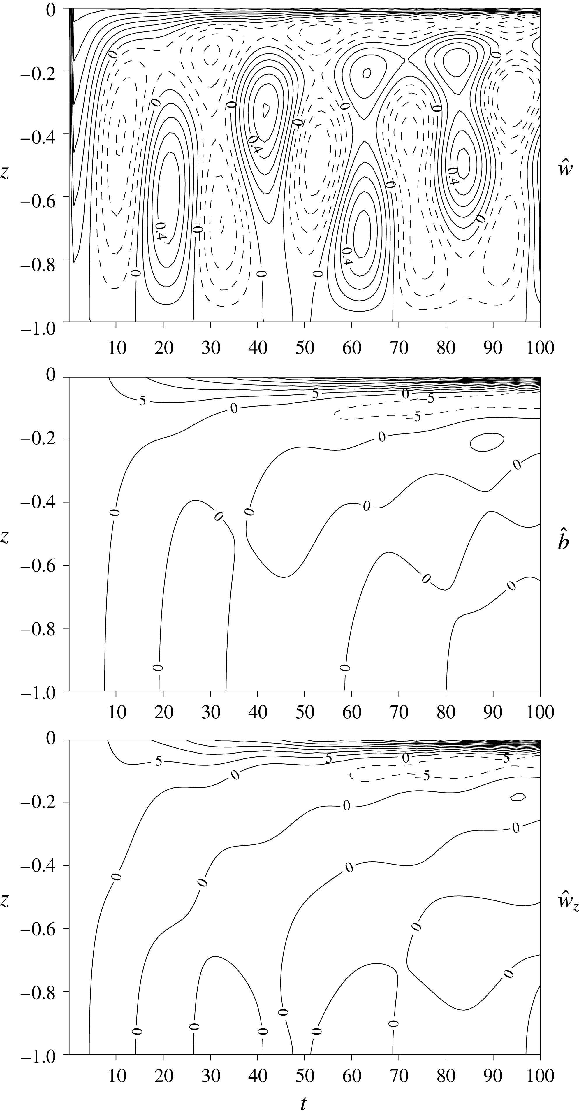
Figures 6 and 7 represent isolines of the functions
 ${\hat{w}}(z,t),\hat{b}(z,t),{\hat{w}}_{z}(z,t)$
(cf. figure 2). The slope of the isolines characterizes the propagation speed of signal: a negative (positive) slope corresponds to downward (upward) propagation. Initial stage of the evolution of the fields is shown in figure 6. At the very initial stage (
 $t<0.5$
) the signals in all fields propagate downwards almost uniformly (the isolines are practically straight lines) and very rapidly; the propagation speed greatly exceeds the maximum group velocity
 $c_{gr}^{max}$
corresponding to the dispersion relation
 $\unicode[STIX]{x1D70E}=\unicode[STIX]{x1D705}/\sqrt{\unicode[STIX]{x1D705}^{2}+m^{2}}$
for (3.19a
) (
 $m$
is the vertical wavenumber in the wave solution
 ${\sim}\text{exp}[\text{i}(mz-\unicode[STIX]{x1D70E}t)]$
, see appendix B). Moreover, the propagation speed tends to infinity as
 $t\rightarrow 0$
. Probably, such a non-standard behaviour is related to the fact that in the boundary value problem (3.19) the lines
 $t=\text{const.}$
and
 $z=\text{const.}$
are characteristics of the hyperbolic equation (3.19a
).
Isolines of the functions
 ${\hat{w}}(z,t),\hat{b}(z,t),{\hat{w}}_{z}(z,t)$
in the time interval [0,5];
 $\unicode[STIX]{x1D705}=1$
,
 $t_{0}=1$
. The dashed straight line corresponds to uniform downward propagation with the maximal group speed
 $c_{gr}^{max}=-2/3\sqrt{3}$
(see appendix B).

Isolines of the functions
 ${\hat{w}}(z,t),\hat{b}(z,t),{\hat{w}}_{z}(z,t)$
in the time interval [0, 100];
 $\unicode[STIX]{x1D705}=1$
,
 $t_{0}=1$
. Contour intervals in the fields
 ${\hat{w}},\hat{b},{\hat{w}}_{z}$
are 0.1, 5, 5 respectively. The dashed isolines are negative.

With increasing time, for
 $t>t_{0}=1$
, the downward propagation of signal moderates and gradually changes into an upward propagation resulting in the formation of boundary layer. Long-term evolution of the BL is represented in figure 7. Contrary to part I the BL presents in all the fields
 ${\hat{w}},\hat{b},{\hat{w}}_{z}$
, and not only in
 $\hat{b},{\hat{w}}_{z}$
. The field
 ${\hat{w}}$
is very similar to the buoyancy field
 $\hat{b}$
from part I (cf. figure 2) excluding the initial stage
 $t\leqslant 1$
. Obviously, this is related to the fact that the problem (2.18), (2.22) for
 $\hat{b}$
coincides (within to a constant multiplier and small initial fields) with the problem (3.15) for
 ${\hat{w}}$
at
 $t>t_{0}$
. At the same time, the boundary layers in
 $\hat{b},{\hat{w}}_{z}$
and in
 ${\hat{w}}$
, are very different in their structure and intensity. The vertical velocity at the surface does not depend on time for
 $t>t_{0}$
, therefore
 ${\hat{w}}$
remains bounded in time, only
 ${\hat{w}}_{z}$
grows in the boundary layer. Isolines of
 ${\hat{w}}(z,t)$
in the boundary layer do not intersect the surface
 $z=0$
and follow along the boundary gradually coming up to it. On the contrary, the fields
 $\hat{b},{\hat{w}}_{z}$
grow
 ${\sim}t$
at
 $z=0$
, therefore the isolines
 $\hat{b}=\text{const.}$
,
 ${\hat{w}}_{z}=\text{const.}$
‘start’ at the surface, slightly displace downwards and then gradually return to the boundary forming the BL. The fields
 $\hat{b},{\hat{w}}_{z}$
below the BL are much weaker than in the BL.
To verify the above asymptotic solutions (3.29), (3.30) and (3.32) we compare them with the exact solutions for
 ${\hat{W}},{\hat{W}}_{z},\hat{B}$
which are readily obtained from (3.24):
 $$\begin{eqnarray}\displaystyle & \displaystyle {\hat{W}}=\frac{1}{t}\int _{0}^{t}{\hat{w}}(t)\,\text{d}t=(z+1)\frac{1}{t}\int _{0}^{t}\hat{F}(t)\,\text{d}t+\frac{1}{t}\mathop{\sum }_{n=1}^{\infty }\sin n\unicode[STIX]{x03C0}z\int _{0}^{t}{\hat{w}}_{n}^{a}\,\text{d}t, & \displaystyle\end{eqnarray}$$
 $$\begin{eqnarray}\displaystyle & \displaystyle {\hat{W}}_{z}=\frac{1}{t}\int _{0}^{t}{\hat{w}}_{z}(t)\,\text{d}t=\frac{1}{t}\int _{0}^{t}\hat{F}(t)\,\text{d}t+\frac{\unicode[STIX]{x03C0}}{t}\mathop{\sum }_{n=1}^{\infty }n\cos n\unicode[STIX]{x03C0}z\int _{0}^{t}{\hat{w}}_{n}^{a}\text{d}t, & \displaystyle\end{eqnarray}$$
 $$\begin{eqnarray}\displaystyle & \displaystyle \hat{B}=\frac{1}{t}\int _{0}^{t}\hat{b}(t)\,\text{d}t=(z+1)\frac{1}{t}\int _{0}^{t}\text{d}t^{\prime }\int _{0}^{t^{\prime }}\hat{F}\text{d}t^{\prime \prime }+\frac{1}{t}\mathop{\sum }_{n=1}^{\infty }\sin n\unicode[STIX]{x03C0}z\int _{0}^{t}\text{d}t^{\prime }\int _{0}^{t^{\prime }}{\hat{w}}_{n}^{a}\,\text{d}t^{\prime \prime }.\qquad & \displaystyle\end{eqnarray}$$
The formulae for
 ${\hat{w}}_{n}^{a}$
and
 ${\hat{W}},{\hat{W}}_{z},\hat{B}$
corresponding to the choice (3.33), (3.34) are rather cumbersome and given in appendix B.
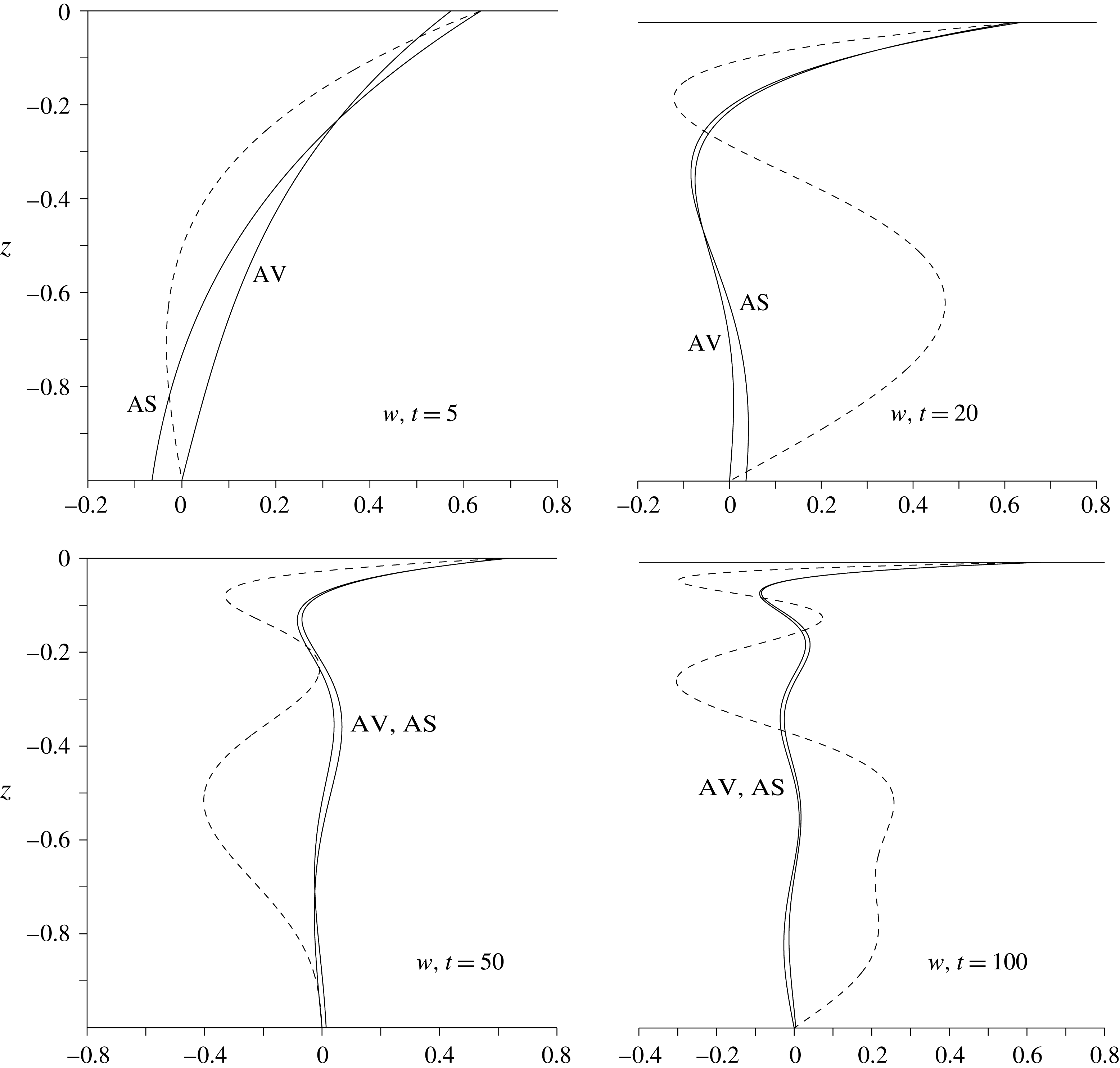
The comparison between the exact and asymptotic solutions is represented in figures 8–10.
The same as in figure 3 but for the vertical velocity
 $w$
in the forced problem.

The correspondence between the solutions is even somewhat better than in part I: the asymptotics (3.29), (3.30), (3.32) describe the exact fields fairly well at
 $t=5$
, and practically coincide with them after
 $t=20$
. As expected, the profiles of the vertical velocity
 ${\hat{W}}$
are very similar to the profiles of the buoyancy
 $\hat{B}$
from part I. The profiles of
 ${\hat{W}}_{z},\hat{B}$
demonstrate a very strong concentration in the BL, much stronger than in part I, because in the BL these quantities grow linearly in time. Due to this growth the surface values of instantaneous fields are two times larger than ones of the time-averaged fields.
The same as in figure 3 but for the buoyancy
 $b$
in the forced problem.

The same as in figure 3 but for the derivative
 $w_{z}$
in the forced problem.

3.5 Effects of viscosity and nonlinearity
In general, the linear solutions discussed above are valid until the viscous and/or nonlinear effects become of importance. Therefore, the ‘large’ times for which the asymptotic solutions remain valid, are still less than the typical nonlinear and viscous time scales. For example, the sharpening vertical gradients should result in that the viscous effects become important in the BL. This means that in equations (3.9a,b
) for the domain outside the friction layer one should take into account the friction terms
 $\unicode[STIX]{x1D700}^{2}u_{0zz}^{in},\unicode[STIX]{x1D700}^{2}v_{0zz}^{in}$
(see (3.4a,b
)). Using (3.30) one can show that at large times
 $$\begin{eqnarray}u_{0t}^{in}\sim \unicode[STIX]{x1D705}\quad \text{and}\quad \unicode[STIX]{x1D700}^{2}u_{0zz}^{in}\sim \unicode[STIX]{x1D700}^{2}\unicode[STIX]{x1D705}^{3}t^{3}.\end{eqnarray}$$
The non-viscous approximation works well if
 $u_{0t}^{in}\gg \unicode[STIX]{x1D700}^{2}u_{0zz}^{in}$
, i.e. if
 $$\begin{eqnarray}\unicode[STIX]{x1D700}^{2}\unicode[STIX]{x1D705}^{2}t^{3}\ll 1.\end{eqnarray}$$
In dimensional form the condition (3.37) is written as
 $$\begin{eqnarray}t^{3}\ll L^{2}/\unicode[STIX]{x1D707}N_{0}^{2},\end{eqnarray}$$
where
 $L=H/\unicode[STIX]{x1D705}$
is the horizontal scale of motion. The condition (3.38) is well satisfied if
 $$\begin{eqnarray}t<T_{\unicode[STIX]{x1D707}}=0.46(L^{2}/\unicode[STIX]{x1D707}N_{0}^{2})^{1/3},\end{eqnarray}$$
i.e. the non-viscous approximation can be considered as valid up to the moment
 $t=T_{\unicode[STIX]{x1D707}}$
. With increasing horizontal scale
 $L$
and decreasing stratification (the buoyancy frequency
 $N_{0}$
) the time
 $T_{\unicode[STIX]{x1D707}}$
increases, i.e. the viscous effect on the wave BL decreases.
Nonlinearity can affect the BL in two ways. First, sufficiently strong vertical shear can become unstable if the corresponding Richardson number
 $Ri=N_{0}^{2}/U_{z}^{2}<0.25$
, where
 $U$
is the horizontal velocity. Second, in the course of time, the nonlinear terms neglected in the governing equations (3.1) will become of the same order as the non-stationary terms
 $u_{t},v_{t},w_{t},b_{t}$
due to the temporal growth of the horizontal velocity and buoyancy. Using the asymptotic solutions (3.29), (3.30) and (3.32) we obtain the following dimensional estimates:
 $$\begin{eqnarray}U_{t}\sim w_{s}N_{0},\quad U_{z}\sim \unicode[STIX]{x1D705}w_{s}N_{0}^{2}t^{2},\quad U_{x}\sim \unicode[STIX]{x1D705}w_{s}N_{0}t,\end{eqnarray}$$
where
 $U$
is any horizontal velocity component (
 $u$
or
 $v$
),
 $w_{s}$
is the typical surface vertical velocity due to external forcing (the exact surface vertical velocity is equal to
 $\int _{0}^{t_{0}}\text{div}\unicode[STIX]{x1D749}\,\text{d}t$
). It follows from these estimates that the nonlinearity ceases to be weak at
 $$\begin{eqnarray}t=T_{non}=(L/w_{s}N_{0})^{1/2},\end{eqnarray}$$
and the instability begins (
 $Ri=0.25$
) somewhat later, at
 $t=\sqrt{2}T_{non}$
. Similar to viscosity, the nonlinear effects on the wave BL decrease with increasing
 $L$
and decreasing
 $N_{0}$
.
For the characteristic geophysical parameters
 $L=10^{3}~\text{m}$
,
 $N_{0}=2\times 10^{-3}~\text{s}^{-1}$
and
 $\unicode[STIX]{x1D707}=10^{-6}~\text{m}^{2}~\text{s}^{-1}$
, the viscous time
 $T_{\unicode[STIX]{x1D707}}\cong 0.3\times 10^{6}~\text{s}\cong 6\times 10^{2}N_{0}^{-1}$
. Estimation of the nonlinear time (3.41) is less reliable because of uncertainty in
 $w_{s}$
. For example, if we assume that typical wind stress
 $\unicode[STIX]{x1D70F}=10^{-4}~\text{m}^{2}~\text{s}^{-2}$
acts during
 $t_{0}=10^{4}~\text{s}$
then the typical
 $w_{s}=10^{-3}~\text{m}~\text{s}^{-1}$
(seems to be too large!) and the nonlinear time
 $T_{non}\cong 2.2\times 10^{4}~\text{s}\cong 40N_{0}^{-1}$
. The estimates demonstrate that wave BL can become well developed before the viscosity and nonlinearity significantly affect it. The same is valid for the BL arising under the boundary of turbulent subsurface layer at which the turbulent momentum fluxes vanish. However it is of importance to note that eventually, for sufficiently long times, the nonlinearity should destroy the BL resulting in strong mixing and instability.
4 Summary and conclusions
We have demonstrated that in a stratified non-rotating fluid there exist non-stationary boundary layers closely resembling those forming near the western shore of ocean in the course of evolution of the forced Rossby waves (see e.g. Lighthill Reference Lighthill1969; Il’in Reference Il’in1970, Reference Il’in1972; Anderson & Gill Reference Anderson and Gill1975; Kamenkovich & Kamenkovich Reference Kamenkovich and Kamenkovich1993). In our case of a continuously stratified fluid confined between two parallel rigid lids the BL is a narrow domain near the fluid surface or/and bottom. The BL width tends to zero and the vertical gradients of at least some fields in the BL tend to infinity as
 $t\rightarrow \infty$
.
The non-stationary BL can arise both as a result of linear evolution of initial perturbation and under the action of an external force (tangential stress exerted on the fluid surface in our case). We have analysed both variants and found that the ‘forced’ BLs are much more intense than the ‘free’ ones. In the ‘free’ BL all fields are bounded and gradients of the buoyancy and horizontal velocity grow linearly in time, whereas in the ‘forced’ BL only the vertical velocity is bounded and the buoyancy and horizontal velocity grow linearly in time. As to the gradients in the ‘forced’ BL, the vertical velocity gradient grows in time linearly and the gradients of buoyancy and horizontal velocity quadratically.
To give an analytical description of BL we used special variables which were introduced originally in Il’in (Reference Il’in1970, Reference Il’in1972), Kamenkovich & Kamenkovich (Reference Kamenkovich and Kamenkovich1993) to study forced Rossby waves: the fields averaged over the interval
 $[0,t]$
for each moment
 $t$
. With these variables we found asymptotic solutions describing development of the non-stationary BL in stratified fluid and compared the solutions with exact solutions written in the form of expansions in the vertical wave modes. The comparison showed that each the BL consists of an infinite number of the internal wave modes with large vertical numbers
 $n\gg 1$
. Therefore we called these boundary layers the wave boundary layers.
It is believed that the existence of a limit point in the frequency spectrum (when the wave frequency tends to a finite limit as the wavenumber tends to infinity) plays an important role in the development of the wave BL. In our case the limit frequency is zero and the wavenumber is vertical (the horizontal wavenumber is fixed); for Rossby waves the limit frequency is also zero but the wavenumber is horizontal. The key point is that the phase and group speeds of waves with large wavenumbers have opposite signs (probably, this is a typical situation when the limit point exists). One can say that the boundary oscillating with the limit frequency acts as a source of a wave signal with phase speeds directed out of the boundary and group speeds directed towards the boundary. Such signals cannot move far from the boundary and form the boundary layer in the course of time. This qualitative scheme is confirmed by the numerical calculations in part II.
With rotation the dispersion relation for internal waves takes the form (see, e.g. Miropol’sky Reference Miropol’sky2001):
 $$\begin{eqnarray}\unicode[STIX]{x1D70E}_{n}=\sqrt{\frac{n^{2}\unicode[STIX]{x03C0}^{2}f^{2}}{n^{2}\unicode[STIX]{x03C0}^{2}+\unicode[STIX]{x1D705}^{2}H^{2}}+\frac{\unicode[STIX]{x1D705}^{2}H^{2}N^{2}}{n^{2}\unicode[STIX]{x03C0}^{2}+\unicode[STIX]{x1D705}^{2}H^{2}}},\end{eqnarray}$$
where
 $f$
is the Coriolis parameter. In this case the inertial frequency
 $f$
is a limiting point of
 $\unicode[STIX]{x1D70E}_{n}$
for fixed
 $\unicode[STIX]{x1D705}$
and
 $n\rightarrow \infty$
. This means that similar wave boundary layers can exist in the field of inertial oscillations. The ‘free’ wave BLs in rotating fluid were considered briefly in Reznik (Reference Reznik2014, Reference Reznik2015) in the context of geostrophic adjustment. More interesting and complicated problem of the ‘forced’ BL in inertial oscillations needs a special examination which will be done elsewhere.
Obviously, the growth of fields and their gradients with time results in a rise of the role of viscosity and nonlinearity in the dynamics of the BL. Estimates show that the viscous and nonlinear effects on the wave BL decrease with increasing
 $L$
and decreasing
 $N_{0}$
, and the BL, under some conditions, can reach a well-developed stage in the presence of these factors. However, one can assume that after a sufficiently long time the nonlinearity should destroy the BL resulting in strong mixing and instability.
The formation of wave BL is an effective linear mechanism of generation of a domain with strong gradients of the buoyancy and horizontal velocity fields, the generation speeding up with increasing buoyancy frequency
 $N$
and the horizontal wavenumber
 $\unicode[STIX]{x1D705}$
. In turn, the sharp gradients can cause instability and mixing in the BL. Such a mechanism, for example, can contribute to formation of the upper homogeneous layer in the ocean and entrainment of the fluid under the layer into a turbulent motion.
For observation of the wave BL in laboratory one can use a tank with a stably stratified fluid. To obtain the ‘free’ BL a horizontally non-uniform surface buoyancy field should be produced at the initial moment. The ‘forced’ BL can be induced by a horizontally non-uniform surface stress exerted on the fluid surface during a finite time.
Acknowledgements
This work was funded by the Russian Science Foundation grant no. 14-50-00095 (part I), the Ministry of Education and Science of Russian Federation grant no. 14.W03.31.0006 (part II) and the Russian Foundation for Basic Research grant no. 17-05-00094 (numerical calculations).
Appendix A
To obtain the initial field
 ${\dot{w}}_{I}$
given
 $b_{I}$
, we express
 $p_{I}$
in terms of
 $b_{I}$
using the equations
 $$\begin{eqnarray}\unicode[STIX]{x1D6FB}^{2}p_{I}=-b_{Iz},\quad p_{Iz}|_{z=0,-1}=b_{I}|_{z=0,-1},\end{eqnarray}$$
which simply follow from equations (2.1), (2.2) written in non-dimensional form with the length scale
 $H$
and the time scale
 $1/N$
. Knowing
 $p_{I}$
we find
 ${\dot{w}}_{I}$
from the vertical momentum equation in (2.1a
):
 $$\begin{eqnarray}{\dot{w}}_{I}=-p_{Iz}-b_{I}.\end{eqnarray}$$
In the case of
 $b_{I}$
given in (2.22) one finds from (A 1):
 $$\begin{eqnarray}p_{I}=\left[\frac{1}{\unicode[STIX]{x1D705}^{2}}-\frac{\text{ch}[\unicode[STIX]{x1D705}(z+1)]}{\unicode[STIX]{x1D705}\text{sh}\unicode[STIX]{x1D705}}\right]\exp [\text{i}(kx+ly)].\end{eqnarray}$$
Substituting (A 3) and (2.22) into (A 2) one obtains:
 $$\begin{eqnarray}\hat{{\dot{w}}}_{I}=\frac{\text{sh}[\unicode[STIX]{x1D705}(z+1)]}{\text{sh}\unicode[STIX]{x1D705}}-(z+1).\end{eqnarray}$$
Now we determine the solutions (2.14), (2.17), (2.19) and (2.36) satisfying the initial conditions (2.22). The solution to (2.13) obeying
 ${\hat{w}}_{I}=0$
and (A 4) can be written as:
 $$\begin{eqnarray}{\hat{w}}=\mathop{\sum }_{n=1}^{\infty }\frac{2\unicode[STIX]{x1D70E}_{n}}{n\unicode[STIX]{x03C0}}\sin \unicode[STIX]{x1D70E}_{n}t\sin n\unicode[STIX]{x03C0}z.\end{eqnarray}$$
The corresponding expansions (2.17), (2.19) for
 $\hat{b},{\hat{w}}_{z}$
are readily derived:
 $$\begin{eqnarray}\hat{b}=z+1+\mathop{\sum }_{n=1}^{\infty }\frac{2}{n\unicode[STIX]{x03C0}}(1-\cos \unicode[STIX]{x1D70E}_{n}t)\sin n\unicode[STIX]{x03C0}z,\end{eqnarray}$$
 $$\begin{eqnarray}{\hat{w}}_{z}=2\mathop{\sum }_{n=1}^{\infty }\unicode[STIX]{x1D70E}_{n}\sin \unicode[STIX]{x1D70E}_{n}t\cos n\unicode[STIX]{x03C0}z.\end{eqnarray}$$
The averaged fields (2.36) simply follow from (A 6), (A 7):
 $$\begin{eqnarray}\displaystyle & \displaystyle {\hat{W}}_{z}=\frac{1}{t}\int _{0}^{t}{\hat{w}}_{z}\,\text{d}t=\frac{2}{t}\mathop{\sum }_{n=1}^{\infty }(1-\cos \unicode[STIX]{x1D70E}_{n}t)\cos n\unicode[STIX]{x03C0}z, & \displaystyle\end{eqnarray}$$
 $$\begin{eqnarray}\displaystyle & \displaystyle \hat{B}=\frac{1}{t}\int _{0}^{t}\hat{b}\,\text{d}t=z+1+\mathop{\sum }_{n=1}^{\infty }\frac{2}{n\unicode[STIX]{x03C0}}\left(1-\frac{\sin \unicode[STIX]{x1D70E}_{n}t}{\unicode[STIX]{x1D70E}_{n}t}\right)\sin n\unicode[STIX]{x03C0}z. & \displaystyle\end{eqnarray}$$
Appendix B
Let us consider the group speed for the wave solution of equation (2.13a
) of the form
 ${\hat{w}}=A\exp [\text{i}(mz-\unicode[STIX]{x1D70E}t)]$
with the dispersion relation
 $\unicode[STIX]{x1D70E}=\unicode[STIX]{x1D705}/\sqrt{\unicode[STIX]{x1D705}^{2}+m^{2}}$
. The corresponding group speed is equal to
 $c_{gr}=\unicode[STIX]{x2202}\unicode[STIX]{x1D70E}/\unicode[STIX]{x2202}m=-m\unicode[STIX]{x1D705}/(\unicode[STIX]{x1D705}^{2}+m^{2})^{3/2}$
and for
 $\unicode[STIX]{x1D705}=1$
it reaches the maximum absolute value
 $|c_{gr}^{max}|=2/3\sqrt{3}$
at
 $m=1/\sqrt{2}$
.
The instantaneous and averaged fields (3.24) and (3.35) are determined by the coefficient
 ${\hat{w}}_{n}^{a}$
in (3.23). First we simplify the integral in (3.23) taking into account (3.25):
 $$\begin{eqnarray}\displaystyle & & \displaystyle \int _{0}^{t}(\hat{F}_{t^{\prime }t^{\prime }}+\hat{F})\sin \unicode[STIX]{x1D70E}_{n}(t-t^{\prime })\,\text{d}t^{\prime }\nonumber\\ \displaystyle & & \displaystyle \quad =\left\{\begin{array}{@{}ll@{}}\displaystyle \unicode[STIX]{x1D70E}_{n}\hat{F}+(1-\unicode[STIX]{x1D70E}_{n}^{2})\int _{0}^{t}\hat{F}\sin \unicode[STIX]{x1D70E}_{n}(t-t^{\prime })\,\text{d}t^{\prime },\quad & t\leqslant t_{0},\\ \displaystyle \hat{F}_{t}(t_{0})\sin \unicode[STIX]{x1D70E}_{n}(t-t_{0})+\unicode[STIX]{x1D70E}_{n}\hat{F}_{0}\cos \unicode[STIX]{x1D70E}_{n}(t-t_{0})\quad \\ \displaystyle +\frac{\hat{F}_{0}}{\unicode[STIX]{x1D70E}_{n}}[1-\cos \unicode[STIX]{x1D70E}_{n}(t-t_{0})]+(1-\unicode[STIX]{x1D70E}_{n}^{2})\int _{0}^{t_{0}}\hat{F}\sin \unicode[STIX]{x1D70E}_{n}(t-t^{\prime })\,\text{d}t^{\prime },\quad & t>t_{0}.\end{array}\right.\end{eqnarray}$$
In the case (3.34) one obtains:
 $$\begin{eqnarray}\displaystyle & & \displaystyle c_{n}=\unicode[STIX]{x1D70E}_{n}\int _{0}^{t}(\hat{F}_{t^{\prime }t^{\prime }}+\hat{F})\sin \unicode[STIX]{x1D70E}_{n}(t-t^{\prime })\,\text{d}t^{\prime }\nonumber\\ \displaystyle & & \displaystyle \quad =\left\{\begin{array}{@{}ll@{}}\displaystyle \frac{\unicode[STIX]{x1D70E}_{n}^{2}(1-\unicode[STIX]{x1D714}^{2})\cos \unicode[STIX]{x1D714}t+\unicode[STIX]{x1D714}^{2}-\unicode[STIX]{x1D70E}_{n}^{2}-\unicode[STIX]{x1D714}^{2}(1-\unicode[STIX]{x1D70E}_{n}^{2})\cos \unicode[STIX]{x1D70E}_{n}t}{\unicode[STIX]{x1D714}(\unicode[STIX]{x1D714}^{2}-\unicode[STIX]{x1D70E}_{n}^{2})},\quad & t\leqslant t_{0},\\ \displaystyle \frac{[\unicode[STIX]{x1D714}^{2}(1+\unicode[STIX]{x1D70E}_{n}^{2})-2\unicode[STIX]{x1D70E}_{n}^{2}]\cos \unicode[STIX]{x1D70E}_{n}(t-t_{0})-\unicode[STIX]{x1D714}^{2}(1-\unicode[STIX]{x1D70E}_{n}^{2})\cos \unicode[STIX]{x1D70E}_{n}t}{\unicode[STIX]{x1D714}(\unicode[STIX]{x1D714}^{2}-\unicode[STIX]{x1D70E}_{n}^{2})}\quad \\ \displaystyle +\frac{2}{\unicode[STIX]{x1D714}}[1-\cos \unicode[STIX]{x1D70E}_{n}(t-t_{0})],\quad & t>t_{0}.\end{array}\right.\end{eqnarray}$$
Using (B 2) one can calculate the coefficients in the expansions (3.24) and (3.35):
 $$\begin{eqnarray}\displaystyle & & \displaystyle {\hat{w}}_{n}^{a}=\frac{2c_{n}}{n\unicode[STIX]{x03C0}},\end{eqnarray}$$
 $$\begin{eqnarray}\displaystyle & & \displaystyle \int _{0}^{t}{\hat{w}}_{n}^{a}\,\text{d}t^{\prime }=\frac{2}{n\unicode[STIX]{x03C0}}\int _{0}^{t}c_{n}\,\text{d}t^{\prime },\end{eqnarray}$$
 $$\begin{eqnarray}\displaystyle & & \displaystyle \int _{0}^{t}\hat{F}(t^{\prime })\,\text{d}t^{\prime }=\frac{1}{\unicode[STIX]{x1D714}}\left\{\begin{array}{@{}ll@{}}t-\sin \unicode[STIX]{x1D714}t/\unicode[STIX]{x1D714},\quad & t\leqslant t_{0},\\ 2t-t_{0},\quad & t>t_{0},\end{array}\right.\end{eqnarray}$$
 $$\begin{eqnarray}\displaystyle & & \displaystyle \int _{0}^{t}c_{n}\,\text{d}t={\displaystyle \frac{1}{\unicode[STIX]{x1D714}(\unicode[STIX]{x1D714}^{2}-\unicode[STIX]{x1D70E}_{n}^{2})}}\nonumber\\ \displaystyle & & \displaystyle \quad \times \left\{\begin{array}{@{}ll@{}}{\displaystyle \frac{\unicode[STIX]{x1D70E}_{n}^{2}(1-\unicode[STIX]{x1D714}^{2})}{\unicode[STIX]{x1D714}}}\sin \unicode[STIX]{x1D714}t+(\unicode[STIX]{x1D714}^{2}-\unicode[STIX]{x1D70E}_{n}^{2})t-{\displaystyle \frac{\unicode[STIX]{x1D714}^{2}(1-\unicode[STIX]{x1D70E}_{n}^{2})}{\unicode[STIX]{x1D70E}_{n}}}\sin \unicode[STIX]{x1D70E}_{n}t,\quad & t\leqslant t_{0},\\ (\unicode[STIX]{x1D714}^{2}-\unicode[STIX]{x1D70E}_{n}^{2})(2t-t_{0})-{\displaystyle \frac{\unicode[STIX]{x1D714}^{2}(1-\unicode[STIX]{x1D70E}_{n}^{2})}{\unicode[STIX]{x1D70E}_{n}}}[\sin \unicode[STIX]{x1D70E}_{n}(t-t_{0})+\sin \unicode[STIX]{x1D70E}_{n}t],\quad & t>t_{0},\end{array}\right.\end{eqnarray}$$
 $$\begin{eqnarray}\displaystyle & & \displaystyle \int _{0}^{t}\text{d}t^{\prime }\int _{0}^{t^{\prime }}\hat{F}(t^{\prime \prime })\,\text{d}t^{\prime \prime }={\displaystyle \frac{1}{\unicode[STIX]{x1D714}}}\left\{\begin{array}{@{}ll@{}}{\displaystyle \frac{t^{2}}{2}}-{\displaystyle \frac{1-\cos \unicode[STIX]{x1D714}t}{\unicode[STIX]{x1D714}^{2}}},\quad & t\leqslant t_{0},\\ t^{2}-tt_{0}+{\displaystyle \frac{t_{0}^{2}}{2}}-{\displaystyle \frac{2}{\unicode[STIX]{x1D714}^{2}}},\quad & t>t_{0},\end{array}\right.\end{eqnarray}$$
 $$\begin{eqnarray}\displaystyle & & \displaystyle \int _{0}^{t}\text{d}t^{\prime }\int _{0}^{t^{\prime }}{\hat{w}}_{n}^{a}\,\text{d}t^{\prime \prime }={\displaystyle \frac{2}{n\unicode[STIX]{x03C0}}}\int _{0}^{t}\text{d}t^{\prime }\int _{0}^{t^{\prime }}c_{n}\,\text{d}t^{\prime \prime },\end{eqnarray}$$
 $$\begin{eqnarray}\displaystyle & & \displaystyle \int _{0}^{t}\text{d}t^{\prime }\int _{0}^{t^{\prime }}c_{n}\,\text{d}t^{\prime \prime }={\displaystyle \frac{1}{\unicode[STIX]{x1D714}(\unicode[STIX]{x1D714}^{2}-\unicode[STIX]{x1D70E}_{n}^{2})}}\nonumber\\ \displaystyle & & \displaystyle \quad \times \left\{\begin{array}{@{}ll@{}}{\displaystyle \frac{\unicode[STIX]{x1D70E}_{n}^{2}(1-\unicode[STIX]{x1D714}^{2})}{\unicode[STIX]{x1D714}^{2}}}(1-\cos \unicode[STIX]{x1D714}t)+(\unicode[STIX]{x1D714}^{2}-\unicode[STIX]{x1D70E}_{n}^{2}){\displaystyle \frac{t^{2}}{2}}\quad \\ \quad -{\displaystyle \frac{\unicode[STIX]{x1D714}^{2}(1-\unicode[STIX]{x1D70E}_{n}^{2})}{\unicode[STIX]{x1D70E}_{n}^{2}}}(1-\cos \unicode[STIX]{x1D70E}_{n}t),\quad & t\leqslant t_{0},\\ {\displaystyle \frac{2[\unicode[STIX]{x1D70E}_{n}^{4}-\unicode[STIX]{x1D714}^{4}+\unicode[STIX]{x1D714}^{2}\unicode[STIX]{x1D70E}_{n}^{2}(\unicode[STIX]{x1D714}^{2}-\unicode[STIX]{x1D70E}_{n}^{2})]}{\unicode[STIX]{x1D714}^{2}\unicode[STIX]{x1D70E}_{n}^{2}}}\quad \\ \quad +(\unicode[STIX]{x1D714}^{2}-\unicode[STIX]{x1D70E}_{n}^{2})\left(t^{2}-t_{0}t+{\displaystyle \frac{t_{0}^{2}}{2}}\right)\quad \\ \quad +{\displaystyle \frac{\unicode[STIX]{x1D714}^{2}(1-\unicode[STIX]{x1D70E}_{n}^{2})}{\unicode[STIX]{x1D70E}_{n}^{2}}}[\cos \unicode[STIX]{x1D70E}_{n}t+\cos \unicode[STIX]{x1D70E}_{n}(t-t_{0})],\quad & t>t_{0}.\end{array}\right.\end{eqnarray}$$