







1 Introduction
The idea to extend the Poisson transform to an operation defined on differential forms goes back to the work [Reference Gaillard12] of P.-Y. Gaillard. He defined a transform on differential forms on a sphere with values in real hyperbolic space of one higher dimension in order to construct differential forms on hyperbolic space which are coclosed and harmonic. This transform is equivariant for the natural actions of
$SO_0(n+1,1)$
 by conformal transformations on
$S^n$
 and by isometries of the hyperbolic metric on hyperbolic space, and representation theory plays an important role in the construction.
It is natural to study the asymptotics of the values of the transform towards infinity and it turns out this depends crucially on the degree of differential forms. For sufficiently small degree, these values admit a smooth extension to the boundary, while for high degrees they diverge towards the boundary. Particularly interesting behaviour occurs in the case that n is odd, for forms whose degree is exactly half the dimension of the interior hyperbolic space. In this case, the transform leads to
$L^2$
 -harmonic forms on hyperbolic space, which only exist in this specific degree. The subspace of
$L^2$
 -harmonic forms is invariant under the action of
$SO_0(n+1,1)$
 and realizes the direct sum of the two discrete series representations of this group with trivial infinitesimal character. Building on Gaillard’s work, J. Lott showed in [Reference Lott22] that these discrete series representations can be identified with spaces of closed forms on the boundary sphere of Sobolev regularity
$H^{-1/2}$
 .
There were several attempts to generalize these methods to the other symmetric spaces of real rank one, i.e. the complex and quaternionic hyperbolic spaces and the octonionic hyperbolic plane. But it quickly turned out that the real case is deceivingly simple. For
$SO_0(n+1,1)$
 there is essentially only one possible transform in each degree, which makes it easy to relate the transform to natural differential operators in the interior. Already in the complex case, corresponding to
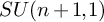
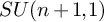
$\operatorname {\mathrm {SU}}(n+1,1)$
 , there are many different choices for Poisson transforms on differential forms, not all of which produce harmonic values, and so on. The question of harmonic values turns out to be very nicely related to the geometry of the sphere in each case. In the complex case, which is mainly considered in this article, one obtains the sphere
$S^{2n+1}$
 with the CR structure coming from the embedding into
$\mathbb {C}^{n+1}$
 . This admits a natural interpretation as the structure on the boundary at infinity of complex hyperbolic space, which is a complete Kähler-Einstein manifold. In the quaternionic case, one obtains a sphere
$S^{4n+3}$
 endowed with a so-called quaternionic contact structure which comes from the embedding into
$\mathbb H^{n+1}$
 . This structure can be interpreted as coming from being a boundary at infinity of quaternionic hyperbolic space, which is a complete quaternion-Kähler manifold, see [Reference Biquard3] for both the complex and the quaternionic case.
The geometries on the spheres one obtains all fall into the class of so-called parabolic geometries, which makes a large set of efficient tools for their study available, see [Reference Čap and Slovák8]. Except for the real case, this structure leads to a refinement of the de Rham complex, which in the complex case is known as the Rumin complex. Writing the sphere as
$G/P$
 for the appropriate semisimple group G and parabolic subgroup
$P\subset G$
 , the representations of P which induce the bundles of differential forms are not completely reducible in this case, but one can form completely reducible subquotients in a natural way. These induce subquotient bundles and there is a construction of natural differential operators (partly of higher order) acting between sections of those. This can be done in such a way that one obtains a complex that computes the de Rham cohomology. This is a very special case of the construction of Bernstein-Gelfand-Gelfand (BGG) sequences, whence we refer to the resulting complexes as BGG complexes. In [Reference Harrach14] it was shown (in a much more general setting) that a Poisson transform for differential forms has harmonic values if and only if it descends to the BGG complex in an appropriate sense, see also Section 2.1 below.
Building on the work in the second author’s thesis [Reference Harrach15], we have constructed in the article [Reference Čap, Harrach and Julg7] Poisson transforms that descend to the BGG complex in the complex case. This was based on an analysis of all possible Poisson transforms and rather extensive computations to find appropriate combinations. In Section 2 of the current article, we use representation theory to devise a construction of appropriate Poisson transforms, which applies to all cases of real rank one (and partly in more generality). In particular, we prove for all cases of real rank one that the values of the resulting transforms are not only harmonic but also coclosed and analyze their compatibility with the exterior derivative on hyperbolic space and the operators in the BGG complex on the sphere.
Starting from Section 3, we specialize to the complex case
$G=\operatorname {\mathrm {SU}}(n+1,1)$
 . In this case, we study harmonic Poisson transforms in detail, analyzing their compatibility with the operations coming from the Kähler structure on complex hyperbolic space. In particular, we show that the transforms in different degrees can be normalized in such a way that one obtains a chain map from the BGG complex on the sphere to the de Rham complex of complex hyperbolic space. Next, we use the Poincaré ball model to realize the sphere as the boundary (at infinity) of complex hyperbolic space and study the boundary asymptotics of the values of the transforms in this picture. This builds on a careful analysis of the restrictions of the transform to isotypic components for the action of the maximal compact subgroup. In particular, we prove that on
$S^{2n+1}$
 , for forms of degree
$\leq n$
 , the values under the transform admit continuous extensions to the boundary. This is in turn used to analyze the composition of d with the transform in degree n, showing in particular that its values are
$L^2$
 -harmonic forms. This leads to Theorem 28, which is the main result of the article: we show that this composition isomorphically embeds the quotient of the degree n part of the BGG complex by the image of the BGG-operator landing in this space onto a dense subspace of the space of
$L^2$
 -harmonic forms of degree
$n+1$
 in the interior, which is known to be the direct sum of the discrete series representations of
$SU(n+1,1)$
 with trivial infinitesimal character.
A major motivation for studying Poisson transforms in our setting is the programme put forward by the third author to use them to prove special cases of the Baum-Connes conjecture with coefficients. We briefly describe this here, referring to [Reference Gomez Aparicio, Julg and Valette13] and [Reference Julg16] for more details.
The Baum-Connes conjecture for a locally compact group G aims to describe the K-theory of the reduced
$C^*$
 -algebra of G in geometrical terms. From the non-commutative geometry point of view, the group
$K_*(C^*_r(G))$
 is the K-theory of the space of unitary representations of G which appear in the left regular representation
$L^2(G)$
 . Baum, Connes and Higson have constructed an assembly map from the K-homology of the classifying space for proper actions of G to the group
$K_*(C^*_r(G))$
 . The conjecture says that this map is an isomorphism. It is important to note that the case where G is a semisimple Lie group is well understood, since representation theory is well understood. See the work of A. Wassermann (using Harish-Chandra theory and the Knapp-Stein intertwining operators) or more recently the beautiful approach of A. Afgoustidis (using D. Vogan’s theory of minimal K-types).
On the other hand, the case of discrete groups is much more problematic, since no theory of representations is available. However, an interesting (and in general still open) problem is the following: given a connected semisimple Lie group G, we would like to prove the Baum-Connes conjecture for any discrete subgroup
$\Gamma $
 of G. This leads to a technical generalization of the conjecture, namely the Baum-Connes conjecture with coefficients for a locally compact group G acting by automorphisms on a
$C^*$
 -algebra A, which is the analogue of the original conjecture for the K-theory groups
$K_*(C^*_r(G,A))$
 . Using the techniques of bivariant K-theory of G. Kasparov, one can show that if a group satisfies BC with coefficients (i.e. for any action on a
$C^*$
 -algebra), then so do all its closed subgroups. This applies to our case: if a connected semisimple group G satisfies the Baum-Connes conjecture with coefficients, then any discrete subgroup
$\Gamma $
 of G satisfies the Baum-Connes conjecture.
We are therefore led to investigate the conjecture with coefficients for connected semisimple Lie groups. Using the geometry of symmetric spaces, Kasparov proves that the assembly map is always injective, and describes the condition for surjectivity in terms of a certain element, denoted
$\gamma $
 , of a ring of bivariant K-theory. More precisely, there is an abelian ring
$KK_G(\mathbb {C},\mathbb {C})$
 which acts by endomorphisms on all the K-theory groups
$K_*(C^*_r(G,A))$
 . Kasparov constructs an idempotent element
$\gamma \in KK_G(\mathbb {C},\mathbb {C})$
 which has the following property: the assembly map to
$K_*(C^*_r(G,A))$
 is surjective if and only if
$\gamma $
 acts by the identity on
$K_*(C^*_r(G,A))$
 .
Let us be a little more precise. An element of
$KK_G(\mathbb {C},\mathbb {C})$
 is a homotopy class of a G-Fredholm module. By a G-Fredholm module, we mean the following data: two Hilbert spaces
$H_0$
 and
$H_1$
 equipped with unitary representations
$\pi _0$
 and
$\pi _1$
 of G, and a Fredholm map
$H_0\rightarrow H_1$
 such that the commutators
$F\pi _0(g)-\pi _1(g)F$
 are compact operators.
The work of many people (J. Fox, P. Haskell, G. Kasparov, Z. Q. Chen and the third author) in the 1980s and 1990s has consisted in constructing an explicit Fredholm module representing the element
$\gamma $
 in the case of the groups
$SO_0(n+1,1)$
 and
$SU(n+1,1)$
 , and eventually proving the conjecture in these cases. The third author has generalized such a construction to
$Sp(n,1)$
 , see [Reference Julg16], and hopes to provide a proof of the BC-conjecture with coefficients for that group. The interesting point is that the unitary representations appearing in the Fredholm module are sums of a finite number of irreducible representations. Those irreducible components are either discrete series or principal series representations. More precisely:
1) The discrete series appearing in the representative of
$\gamma $
 are the components of the
$L^2$
 -cohomology of the symmetric space
$G/K$
 , i.e. the Hilbert space of square-integrable harmonic forms on
$G/K$
 . They are absent for
$G=SO_0(2n+1,1)$
 ; there are 2 components in the case of
$SO_0(2n,1)$
 and
$n+2$
 components in the cases of
$SU(n+1,1)$
 and
$Sp(n+1,1)$
 .
2) The principal series appearing in
$\gamma $
 are also very specific ones. In the case of
$SO_0(n+1,1)$
 , they are exactly the differential forms on the boundary sphere
$G/P$
 (made unitary after twisting by some density line bundle). But the general case is more subtle. Let us explain that: let
$P=MAN$
 be the Iwasawa decomposition of the parabolic group P. A principal series representation is induced from P to G of a representation of P which is trivial on the nilpotent group N (equivalently a representation of
$M\times A$
 ). The representation of G on the spaces of differential forms splits into principal series if and only if the adjoint action of N on its Lie algebra is trivial, i.e. iff N is abelian. This is the case for
$SO_0(n+1,1)$
 since N is isomorphic to
$\mathbb {R}^n$
 , but not for
$SU(n+1,1)$
 where N is the Heisenberg group
$\mathbb {C}^n\oplus i\mathbb {R}$
 . The same occurs in the case of
$Sp(n+1,1)$
 , where
$N = \mathbb {H}^n \oplus \operatorname {\mathrm {im}}(\mathbb {H})$
 . This forces us to replace the bundle of forms on
$G/P$
 by a subquotient on which the action of N is trivial: this means exactly to replace the de Rham complex by the BGG complex.
The last ingredient in the construction of the G-Fredholm module is a Poisson map between the BGG complex on
$G/P$
 (more precisely the component below the middle) and the
$L^2$
 -harmonic forms of
$G/K$
 . In the
$SO_0(n+1,1)$
 case this is exactly the map from
$\Omega ^n(G/P)$
 to
$\Omega ^{n+1}(G/K)$
 given by composition of P.-Y. Gaillard’s Poisson transform in degree n with the de Rham operator on
$G/K$
 as mentioned above. In the current paper, we sort out the case of
$\operatorname {\mathrm {SU}}(n+1,1)$
 , and make precise the link with the computations in [Reference Julg and Kasparov17]. As mentioned above, Section 2 provides several ingredients needed for attacking the case of
$Sp(n+1,1)$
 .
2 General theory of Poisson transforms
2.1 Harmonic Poisson transforms
Throughout this section let
$\mathfrak {g}$
 be a non-compact real semisimple Lie algebra with Cartan involution
$\theta $
 and corresponding Cartan decomposition
$\mathfrak {g} = \mathfrak {k} \oplus \mathfrak {q}$
 so that
$\mathfrak {q} \neq \{0\}$
 . Choose a maximal abelian subspace
$\mathfrak {a}_0 \subset \mathfrak {q}$
 and let
$\Delta _r \subset \mathfrak {a}_0^*$
 be the set of restricted roots of
$\mathfrak {g}$
 with respect to
$\mathfrak {a}_0$
 . For
$\lambda \in \Delta _r$
 let
$\mathfrak {g}_{\lambda }$
 be its restricted root space and define
$\mathfrak {m}_0$
 as the centralizer of
$\mathfrak {a}_0$
 in
$\mathfrak {k}$
 . Choose subsets
$\Delta _r^+$
 and
$\Sigma _0$
 of positive and simple roots, respectively, and let
$\mathfrak {n}_0 = \bigoplus _{\lambda \in \Delta _r^+} \mathfrak {g}_{\lambda }$
 . Then
$\mathfrak {p}_0 := \mathfrak {m}_0 \oplus \mathfrak {a}_0 \oplus \mathfrak {n}_0$
 is a Borel subalgebra of
$\mathfrak {g}$
 . Let
$\mathfrak {p}$
 be a standard parabolic subalgebra of
$\mathfrak {g}$
 with respect to
$\mathfrak {p}_0$
 and let
$\Sigma \subset \Sigma _0$
 be its corresponding subset of simple roots. Let
$\mathfrak {g} = \mathfrak {g}_{-k} \oplus \dotso \oplus \mathfrak {g}_k$
 be the
$|k|$
 -grading of
$\mathfrak {g}$
 induced by
$\Sigma $
 -height. Define
$\mathfrak {p}_+$
 and
$\mathfrak {g}_-$
 to be the sum of all positive and negative grading components, respectively; then by construction, we have
$\mathfrak {p} = \mathfrak {g}_0 \oplus \mathfrak {p}_+$
 . Put
$\mathfrak {m} := \mathfrak {k} \cap \mathfrak {p} = \mathfrak {k} \cap \mathfrak {g}_0$
 as well as
$\mathfrak {a} := \mathfrak {q} \cap \mathfrak {g}_0$
 . Let G be a connected semisimple Lie group with Lie algebra
$\mathfrak {g}$
 and assume that the centre of G is finite. Let K be the maximal compact subgroup with Lie algebra
$\mathfrak {k}$
 ,
$P = N_G(\mathfrak {p})$
 be the parabolic subgroup of G with Lie algebra
$\mathfrak {p}$
 and let
$P_+ \subset P$
 be its unipotent radical whose Lie algebra coincides with
$\mathfrak {p}_+$
 . We identify the quotient group
$G_0 := P/P_+$
 with a subgroup of G so that the Lie algebra of
$G_0$
 coincides with
$\mathfrak {g}_0$
 .
We briefly recall the construction of a G-equivariant operator mapping between vector-valued differential forms on
$G/P$
 and
$G/K$
 as presented in [Reference Harrach14], see also [Reference Harrach15]. The Iwasawa decomposition yields a diffeomorphism
$G/M \cong G/K \times G/P$
 of G-manifolds, where
$M := K \cap P$
 . Denoting the natural projections from
$G/M$
 to
$G/K$
 and
$G/P$
 by
$\pi _K$
 and
$\pi _P$
 , respectively, we obtain an induced decomposition of the tangent bundle of
$G/M$
 into the direct sum of
$T_K := \ker (T\pi _P)$
 and
$T_P := \ker (T\pi _K)$
 . Next, for an irreducible G-representation
$\mathbb {V}$
 and a closed subgroup H of G we denote by
$V_H := G \times _H \mathbb {V}$
 its associated vector bundle over
$G/H$
 . Now for another irreducible G-representation
$\mathbb {W}$
 we obtain a decomposition

where the elements in
$\Lambda ^{k_1,k_2}$
 vanish unless exactly
$k_1$
 of their entries come from
$T_K$
 and the remaining
$k_2$
 entries are from
$T_P$
 .
Assuming that
$G/P$
 is oriented and
$\dim (G/P) = N$
 , we fix a G-invariant
$(0,N)$
 -form
$\operatorname {\mathrm {vol}}_M$
 on
$G/M$
 , which is unique up to multiples, and normalize it so that the fibre
$\pi _K^{-1}(eK)$
 has unit volume. Then each G-equivariant bundle map

induces, via integration along fibers, a G-equivariant integral operator

called a Poisson transform. Equivalently, any such bundle map induces a G-invariant differential form
$\varphi $
 of bidegree
$(\ell , N-k)$
 on
$G/M$
 with values in
$L(V_M, W_M)$
 via the relation

For each closed subgroup H of G the homogeneous bundle
$V_H = G \times _H \mathbb {V}$
 carries a canonical G-invariant flat connection
$\nabla ^{V_H}$
 , which induces a covariant exterior derivative
$d^{V_H}$
 on
$\Omega ^*(G/H, V_H)$
 in the usual way. Additionally, we can find an inner product on
$\mathbb {V}$
 so that
$\langle X v_1, v_2 \rangle = \langle v_1, \theta (X) v_2\rangle $
 for all
$X \in \mathfrak {g}$
 and
$v_1$
 ,
$v_2 \in \mathbb {V}$
 . By construction, this inner product is K-invariant and thus yields a G-invariant bundle metric on
$V_K \to G/K$
 . Next, we define
$\nabla ^{\theta }$
 as the dual connection to
$\nabla ^{V_K}$
 with respect to this bundle metric, which is again flat. Moreover, we obtain an induced covariant exterior derivative
$d^{\theta }$
 on
$\Omega ^*(G/K,V_K)$
 and we define
$\delta ^{V_K}$
 as the formal adjoint of
$d^{\theta }$
 with respect to the induced
$L^2$
 -norm. Finally, define the Laplace operator
$\Delta ^{V_K}$
 via
$\Delta ^{V_K} := \delta ^{V_K}d^{V_K} + d^{V_K}\delta ^{V_K}$
 . In [Reference Harrach14, Theorem 6] the following was proven.
Proposition 1. For each Poisson transform
$\Phi \colon \Omega ^k(G/P, V_P)\to \Omega ^\ell (G/K, W_K)$
 the compositions
$\Phi \circ d^{V_P}$
 ,
$d^{W_K} \circ \Phi $
 ,
$\delta ^{W_K} \circ \Phi $
 and
$\Delta ^{W_K} \circ \Phi $
 are again Poisson transforms.
In the next step we recall the BGG-calculus on
$G/P$
 and afterwards consider Poisson transforms which are naturally linked to BGG complexes. Consider the standard complex
$(C^*(\mathfrak {g}_-, \mathbb {V}), \mathfrak {d})$
 for computing Lie algebra cohomology of the nilpotent Lie algebra
$\mathfrak {g}_-$
 with values in a
$\mathfrak {g}$
 -representation
$\mathbb {V}$
 . Each chain space is naturally a
$G_0$
 -module, and the differentials are
$G_0$
 -equivariant. On the other hand, under the identification
$\mathfrak {g}_-^* \cong \mathfrak {p}_+$
 the Kostant codifferential
$\mathfrak {d}^* \colon C^k(\mathfrak {g}_-, \mathbb {V}) \to C^{k-1}(\mathfrak {g}_-, \mathbb {V})$
 introduced originally in [Reference Kostant20] is defined via

for all
$Z_i \in \mathfrak {p}_+$
 and
$v \in \mathbb {V}$
 , where the hat denotes omission. It is immediate that this map is P-equivariant and squares to zero. Therefore, the induced homology spaces
$H_k := H_k(\mathfrak {p}_+, \mathbb {V}) := \ker (\mathfrak {d}^*)/\operatorname {\mathrm {im}}(\mathfrak {d}^*)$
 are naturally P-modules which are completely reducible, c.f. [Reference Čap and Slovák8, Corollary 3.3.1]. Let
$\Box = \mathfrak {d} \mathfrak {d}^* + \mathfrak {d}^* \mathfrak {d}$
 be the Kostant Laplacian on
$C^k(\mathfrak {g}_-, \mathbb {V})$
 , which is
$G_0$
 -equivariant. We obtain a
$G_0$
 -invariant decomposition

and the sums of the first two and the last two summands coincide with
$\ker (\mathfrak {d})$
 and
$\ker (\mathfrak {d}^*)$
 , respectively. In particular, the homology spaces
$H_k$
 are isomorphic to
$\ker (\Box )$
 as
$G_0$
 -modules.
Denote the G-equivariant bundle map on
$\Lambda ^* T^*(G/P)\otimes V_P$
 induced by
$\mathfrak {d}^*$
 by the same symbol. Moreover, let
$\mathcal {H}_k = \mathcal {H}_k(G/P, V_P)$
 be the homogeneous vector bundle over
$G/P$
 associated to
$H_k$
 . Since the operator
$\Box $
 is
$G_0$
 -equivariant, we obtain an induced tensorial operator on the associated graded of
$\Lambda ^k T^*(G/P)\otimes V_P$
 , and the decomposition (4) globalizes only to this space. To remedy this fact, let
$\Box ^R := d^{V_P}\mathfrak {d}^* + \mathfrak {d}^* d^{V_P}$
 be the curved Box operator; then from [Reference Calderbank and Diemer6, Theorem 5.2] we know that
$\Box ^R$
 is invertible on sections of the subbundle induced by
$\operatorname {\mathrm {im}}(\mathfrak {d}^*)$
 , and the inverse
$Q^R$
 can be written as a universal polynomial in
$\mathfrak {d}^*d^{V_P}$
 by [Reference Čap and Souček11, Theorem 3.9]. Using this, it can be shown that

(c.f. [Reference Harrach14, p. 24]) and the projection
$\Pi ^R \colon \Omega ^k(G/P, V_P) \to \ker (\Box ^R)$
 onto the middle summand is given by

for all
$\alpha \in \Omega ^k(G/P, V_P)$
 . From the definition of
$Q^R$
 , one easily concludes that (6) implies
$\mathfrak {d}^* \circ \Pi ^R = 0$
 . In particular,
$\Pi ^R$
 factors to an operator
$L \colon \Gamma (\mathcal {H}_k) \to \Gamma (\ker (\mathfrak {d}^*))$
 , which is a G-equivariant splitting operator for the canonical projection
$\pi _{\mathcal {H}}:\Gamma (\ker (\mathfrak {d}^*))\to \Gamma (\mathcal {H}_k)$
 and it is characterized by
$\mathfrak {d}^*d^{V_P}L = 0$
 . We define the k-th BGG-operator
$D_k \colon \Gamma (\mathcal {H}_{k-1}) \to \Gamma (\mathcal {H}_k)$
 as the composition
$D_k := \pi _{\mathcal {H}} d^{V_P} L$
 . Since the connection
$\nabla ^{V_P}$
 on
$V_P$
 is flat, it follows that the BGG-sequence

is a complex which computes the twisted de Rham cohomology of
$G/P$
 with values in the vector bundle
$V_P$
 , c.f. [Reference Čap, Slovák and Souček9, Corollary 4.15].
Our aim is to construct Poisson transforms which satisfy
$\Phi \circ \mathfrak {d}^* = 0$
 as well as
$\Phi \circ d^{V_P} \circ \mathfrak {d}^* = 0$
 . By the first property,
$\Phi $
 naturally factors to an operator
$\underline {\Phi } \colon \Gamma (\mathcal {H}_k) \to \Omega ^\ell (G/K, W_K)$
 defined by
$\underline {\Phi }(\sigma ) := \Phi (\alpha )$
 , where
$\alpha \in \Gamma (\ker (\mathfrak {d}^*))$
 is any representative of
$\sigma \in \Gamma (\mathcal {H}_k)$
 . The second property yields compatibility with the k-th BGG-operator, i.e. for all
$\tau \in \Gamma (\mathcal {H}_{k-1})$
 the value
$\underline {\Phi }(D_k\tau )$
 coincides with
$\Phi (d^{V_P}\beta )$
 for any representative
$\beta \in \Gamma (\ker (\mathfrak {d}^*))$
 of
$\tau $
 , c.f. [Reference Harrach14, Section 3.1].
In order to relate the BGG complex to the geometry of
$G/K$
 , recall that for each homogeneous vector bundle
$E \to G/H$
 we have a natural G-action on
$\Gamma (E)$
 . Infinitesimally, one obtains an action of the universal enveloping algebra
$\mathcal {U}(\mathfrak {g})$
 on sections of E, so in particular the Casimir element
$\mathcal {C} \in \mathcal {U}(\mathfrak {g})$
 induces a G-invariant differential operator
$\Gamma (E) \to \Gamma (E)$
 which we denote by the same symbol.
Theorem 2. Let
$\Phi \colon \Omega ^k(G/P, V_P) \to \Omega ^{\ell }(G/K, W_K)$
 be a Poisson transform.
-
(i) Let $c_{\mathbb {V}}$
 and
$c_{\mathbb {W}}$
be the Casimir eigenvalues of
$\mathbb {V}$
and
$\mathbb {W}$
, respectively. Then $$ \begin{align*} 2\Phi(\Box^R\alpha) + \Delta^{W_K}\Phi(\alpha) = (c_{\mathbb{W}} - c_{\mathbb{V}}) \Phi(\alpha). \end{align*} $$
In particular, if $\Phi \circ \Box ^R = 0$
, then for any
$\alpha \in \Omega ^k(G/P,V_P)$
the element
$\Phi (\alpha )$
is an eigenform of
$\Delta ^{W_K}$
with eigenvalue
$(c_{\mathbb {W}} - c_{\mathbb {V}})$
, or equivalently, an eigenform of
$\mathcal {C}$
with eigenvalue
$c_{\mathbb {V}}$
. -
(ii) The following are equivalent:
-
(a) $\Phi \circ \Box ^R = 0$
, -
(b) $\Phi \circ \mathfrak {d}^* = 0$
and
$\Phi \circ d^{V_P} \circ \mathfrak {d}^* = 0$
, -
(c) $\Phi = \Phi \circ \Pi ^R$
.
If these are satisfied, $\Phi $
is uniquely determined by its induced operator
$\underline {\Phi }$
on
$\Gamma (\mathcal {H}_k)$
. -


Proof. (i) From [Reference Čap and Souček10, Corollary 1] we know that on
$\Omega ^k(G/P, V_P)$
 we have
$\mathcal {C} = 2 \Box ^R + c_{\mathbb {V}}$
 . On the other hand, in [Reference Matsushima and Murakami25, p. 385, formula (6.9)] it was proven that
$\mathcal {C} = -\Delta ^W + c_{\mathbb {W}}$
 on
$\Omega ^*(G/K, W_K)$
 . Since Poisson transforms are G-equivariant, they commute with
$\mathcal {C}$
 , implying the claim.
(ii) The decomposition (5) immediately implies the equivalence of
$(b)$
 and
$(c)$
 , whereas the equivalence of
$(a)$
 and
$(b)$
 was shown in [Reference Harrach14, Theorem 4]. Finally, for the uniqueness result note that the splitting operator is an isomorphism
$\Gamma (\mathcal {H}_k) \to \Gamma (\ker (\Box ^R))$
 and satisfies
$\underline {\Phi } = \Phi \circ L$
 .
Part (i) of the previous theorem shows that for
$\mathbb {W} = \mathbb {V}$
 the condition
$\Phi \circ \Box ^R = 0$
 is equivalent to
$\Delta ^{V_K} \circ \Phi = 0$
 . In light of this we have the following definition.
Definition 1. We say that a Poisson transform
$\Phi \colon \Omega ^k(G/P,V_P) \to \Omega ^{\ell }(G/K, W_K)$
 is harmonic if it satisfies one of the three equivalent properties of part (ii) in Theorem 2.
2.2 BGG-compatibility and equivariant maps
A crucial feature of the approach to Poisson transforms introduced above is that, in view of the homogeneity of
$G/M$
 , G-equivariant bundle maps as in (1) are in bijective correspondence with M-equivariant maps between the representations inducing the bundles. We next describe harmonic Poisson transforms in this language.
We start with some general observations. Since
$M=K\cap P$
 , any representation
$\mathbb {V}$
 of K restricts to a representation of M and hence gives rise to a homogeneous bundle
$G\times _M\mathbb {V}\to G/M$
 , which can be identified with the pullback along
$\pi _K$
 of the homogeneous bundle
$G\times _K\mathbb {V}\to G/K$
 . Natural bundle maps between homogeneous bundles over
$G/K$
 come from K-equivariant maps between the inducing representations and hence lift to natural bundle maps between the pullback bundles. This also applies to the projection to
$G/P$
 , but in this case, more is true. Since
$M\subset G_0\subset P$
 , also representations of
$G_0$
 give rise to natural bundles over
$G/M$
 , and
$G_0$
 -equivariant maps induce natural bundle maps between such homogeneous bundles. In the case of representations of
$G_0$
 which are not restrictions of representations of P, one has to be careful with the pullback interpretation, though. This is available for associated bundles to the principal
$G_0$
 -bundle
$G/P_+\to G/P$
 which can be interpreted as homogeneous bundles corresponding to completely reducible representations of P.
The M-representation inducing
$T(G/M)$
 is
$\mathfrak {g}/\mathfrak {m}$
 . The subbundle
$T_K$
 corresponds to
$(\mathfrak {g}/\mathfrak {m})^{1,0} := \mathfrak {p}/\mathfrak {m}$
 , which is isomorphic to the restriction to M of the K-representation
$\mathfrak {g}/\mathfrak {k}$
 . Likewise,
$T_P$
 corresponds to
$(\mathfrak {g}/\mathfrak {m})^{0,1} := \mathfrak {k}/\mathfrak {m}$
 , which is isomorphic to the restriction of the P-representation
$\mathfrak {g}/\mathfrak {p}$
 . For the induced decomposition of the dual, there is a more natural point of view as
$(\mathfrak {g}/\mathfrak {m})^*=(\mathfrak {g}/\mathfrak {k})^*\oplus (\mathfrak {g}/\mathfrak {p})^*$
 . Viewing
$(\mathfrak {g}/\mathfrak {m})^*$
 as the annihilator of
$\mathfrak {m}$
 in
$\mathfrak {g}^*$
 , the summands are naturally contained as annihilators of bigger subalgebras. Hence
$\Lambda ^{k_1,k_2} (\mathfrak {g}/\mathfrak {m})^* := \Lambda ^{k_1} (\mathfrak {g}/\mathfrak {k})^* \otimes \Lambda ^{k_2} (\mathfrak {g}/\mathfrak {p})^*$
 is the M-module underlying
$\Lambda ^{k_1,k_2} T^*(G/M)$
 . The above observations on restrictions of
$G_0$
 -representations to M apply to the chain spaces
$C^k(\mathfrak {g}_-, \mathbb {V})$
 and the equivariant maps
$\mathfrak {d}$
 ,
$\mathfrak {d}^*$
 and
$\Box $
 , for which we denote the induced natural bundle maps by
$\mathfrak {d}_P$
 ,
$\mathfrak {d}_P^*$
 and
$\Box _P$
 . The splitting (4) then reads as

and the sum of the first and last two modules coincide with
$\ker (\mathfrak {d}_P)$
 and
$\ker (\mathfrak {d}_P^*)$
 , respectively. Finally,
$H_k = H_k(\mathfrak {p}_+, \mathbb {V})\cong _M\ker (\Box _P)$
 , so over
$G/M$
 we can identify
$\Gamma (\mathcal {H}_k)$
 with
$\Gamma (\ker (\Box _P))$
 , and its elements are described by M-equivariant maps
$G\to \ker (\Box _P)$
 .
Theorem 3. Let
$\Phi \colon \Omega ^k(G/P, V_P) \to \Omega ^{\ell }(G/K, W_K)$
 be a Poisson transform.
-
(i) The compositions $\Phi \circ \mathfrak {d}^*$
and
$\Phi \circ \Pi ^R$
are again Poisson transforms. -
(ii) If $\Phi \circ \mathfrak {d}^* = 0$
, then
$\Psi := \Phi \circ \Pi ^R$
is a harmonic Poisson transform which induces the same transform on
$\Gamma (\mathcal {H}_k)$
as
$\Phi $
. Moreover, if
$\sigma \in \Gamma (\mathcal {H}_k)$
corresponds to
$\underline {\sigma } \in \Gamma (\ker (\Box _P))$
, then where $\psi $
is the M-equivariant map underlying
$\Psi $
. Therefore, harmonic Poisson transforms are in bijective correspondence with
$\operatorname {\mathrm {Hom}}_M(\ker (\Box _P), \Lambda ^{\ell ,0}(\mathfrak {g}/\mathfrak {m})^* \otimes \mathbb {W})$
.


Proof. (i) By construction,
$\mathfrak {d}_P^*\pi _P^*\alpha $
 coincides with
$\pi _P^*\mathfrak {d}^*\alpha $
 for all
$\alpha \in \Omega ^k(G/P, V_P)$
 , and thus
$\Phi \circ \mathfrak {d}^*$
 is a Poisson transform. Since
$\Phi \circ d^{V_P}$
 is a Poisson transform due to Proposition 1, the same is true for
$\Phi \circ \Pi ^R$
 as
$\Pi ^R$
 is a polynomial in
$\mathfrak {d}^*d^{V_P}$
 .
(ii) From Theorem 2(ii), we know that the operator
$\Psi = \Phi \circ \Pi ^R$
 is harmonic. Moreover, given
$\sigma \in \Gamma (\mathcal {H}_k)$
 with representative
$\alpha \in \Gamma (\ker (\mathfrak {d}^*))$
 , then
$\Pi ^R(\alpha )$
 is also a representative of
$\sigma $
 . This implies that the maps induced by
$\Phi $
 and
$\Psi $
 on
$\Gamma (\mathcal {H}_k)$
 coincide, and uniqueness follows directly from Theorem 2(ii). Next,
$\Psi \circ \mathfrak {d}^* = 0$
 implies that
$\psi $
 is trivial on
$\operatorname {\mathrm {im}}(\mathfrak {d}_P^*)$
 , so from the decomposition (7) it is immediate that
$\psi (\pi _P^*\alpha )$
 coincides with
$\psi (\underline {\sigma })$
 . This also shows that
$\Psi $
 is fully determined by the restriction of
$\psi $
 to
$\ker (\Box _P)$
 .
Recall that for any G-representation
$\mathbb {V}$
 , the homology space
$H_k = H_k(\mathfrak {p}_+, \mathbb {V})$
 decomposes into a direct sum of irreducible P-representations
$\mathbb {E}_i^k$
 and we denote by
$\pi ^k_i$
 the projection onto the component
$\mathbb {E}_i^k$
 . In the same way, the M-representation
$\ker (\Box _P)$
 decomposes into irreducible components that we also denote by
$\mathbb {E}_i^k$
 . Correspondingly
$\mathcal {H}_k = G \times _P H_k=\oplus _iE_i^k$
 , where
$E_i^k := G \times _P \mathbb {E}_i^k$
 , and the projection onto one summand is a G-equivariant bundle map. We also denote this bundle map and the induced tensorial operator on sections by
$\pi _i^k$
 . This leads to a splitting of the kth BGG-operator into components
$D^{j,i}_k$
 defined by
$D^{j,i}_k := \pi _i^k \circ D_k\circ \pi _j^{k-1}$
 .
Now suppose that we are given a harmonic Poisson transform
$\Phi :\Omega ^k(G/P,V_P)\to \Omega ^\ell (G/K,W_K)$
 induced by
$\phi \in \operatorname {\mathrm {Hom}}_M(\ker (\Box _P), \Lambda ^{\ell ,0} (\mathfrak {g}/\mathfrak {m})^*\otimes \mathbb {W})$
 . Then we define
$\phi _i:=\phi \circ \pi _i^k$
 and this induces a harmonic Poisson transform
$\Phi _i$
 acting between the same spaces as
$\Phi $
 . Part (ii) of Theorem 3 readily shows that for the induced transform we get
$\underline {\Phi }_i=\underline {\Phi }\circ \pi _i^k$
 . Using this, we can now show that harmonic Poisson transforms are well behaved with respect to compositions with components of BGG-operators.
Proposition 4. Let
$\Phi \colon \Omega ^k(G/P,V_P) \to \Omega ^{\ell }(G/K, W_K)$
 be a harmonic Poisson transform and let
$\Phi _i$
 be the component corresponding to
$E_i^k \subset \mathcal {H}_k$
 . Consider the kth BGG-operator
$D_k$
 and a component
$D^{j,i}_k$
 with values in
$\Gamma (E_i^k)$
 .
-
(i) The transform $\underline {\Phi }\circ D$
on
$\Gamma (\mathcal {H}_{k-1})$
is induced by a harmonic Poisson transform defined on
$\Omega ^{k-1}(G/P,V_P)$
. -
(ii) Let $\Psi $
be a harmonic Poisson transform which in the setting of (i) induces
$\underline {\Phi }_i\circ D$
. Then the harmonic Poisson transform
$\Psi _j$
induces
$\underline {\Phi }\circ D^{i,j}_k:\Gamma (\mathcal {H}_{k-1})\to \Omega ^{\ell }(G/K, W_K)$
.


Proof. (i) By definition of the BGG-operators, for any
$\alpha \in \Gamma (\mathcal {H}_{k-1})$
 , the differential form
$d^{V_P}(L(\alpha ))$
 is a representative for
$D(\alpha )\in \Gamma (\mathcal {H}_k)$
 , and hence
$\Phi \circ d^{V_P}\circ \Pi ^R$
 induces
$\underline {\Phi }\circ D$
 on homology bundles. Now
$\Phi \circ d^{V_P}$
 is a Poisson transform by Proposition 1, and since
$\Phi $
 is harmonic, we get
$(\Phi \circ d^{V_P})\circ \mathfrak {d}^*=0$
 . By part (i) of Theorem 3 this implies that
$\Phi \circ d^{V_P}\circ \Pi ^R$
 is a harmonic Poisson transform.
(ii) By construction, we have
$\underline {\Psi }(\beta )=\underline {\Phi }(\pi ^k_iD(\beta ))$
 and
$\underline {\Psi }_j(\beta )=\underline {\Psi }(\pi^{k-1}_j(\beta ))$
 , which implies the claim.
2.3 A specific family of transforms
We now specialize to a family of transforms that will be used in what follows. We do this only in the case that
$\mathbb {V}$
 and
$\mathbb {W}$
 are
$\mathbb {R}$
 or
$\mathbb {C}$
 and that
$\mathfrak {g}$
 is of real rank one. This implies that
$\mathfrak {p}\subset \mathfrak {g}$
 is a minimal parabolic subalgebra and that
$\mathfrak {a}=\mathfrak {q}\cap \mathfrak {g}_0$
 is a one-dimensional abelian subalgebra spanned by the grading element E. This element is characterized by
$[E, X] = jX$
 for all
$X \in \mathfrak {g}_j$
 , which implies that M acts trivially on
$\mathfrak {a}$
 .
It is well known that
$\mathfrak {p}_+$
 is the annihilator of
$\mathfrak {p}$
 under the Killing form B, so one obtains an isomorphism
$(\mathfrak {g}/\mathfrak {p})^*\cong \mathfrak {p}_+$
 . This is P-equivariant and hence M-equivariant and thus can also be viewed as an isomorphism
$\Lambda ^{0,1}(\mathfrak {g}/\mathfrak {m})^*\cong _M\mathfrak {p}_+$
 . Similarly,
$\mathfrak {q}$
 is the annihilator of
$\mathfrak {k}$
 under the Killing form, so we get an isomorphism
$(\mathfrak {g}/\mathfrak {k})^*\cong \mathfrak {q}$
 . This is K-equivariant and hence M-equivariant, so
$\Lambda ^{1,0}(\mathfrak {g}/\mathfrak {m})^*\cong _M\mathfrak {q}$
 . But now
$\mathfrak {q}\cap (\mathfrak {g}_-\oplus \mathfrak {p}_+)$
 is an M-invariant complement to
$\mathfrak {a}$
 in
$\mathfrak {q}$
 , and any element in there can be uniquely written as
$\theta (Z)-Z$
 for some
$Z\in \mathfrak {p}_+$
 . Thus, we conclude that
$\Lambda ^{1,0}(\mathfrak {g}/\mathfrak {m})^*\cong \mathfrak {a}\oplus \mathfrak {p}_+$
 as a representation of M. Otherwise put, sending
$Z\in \mathfrak {p}_+$
 to the map
$Y\mapsto B(Y,\theta (Z)-Z)$
 defines an M-equivariant injection
$\mathfrak {p}_+\to \Lambda ^{1,0}(\mathfrak {g}/\mathfrak {m})^*$
 . Together with the above, this defines an M-equivariant injection
$\iota _1:\Lambda ^{0,1}(\mathfrak {g}/\mathfrak {m})^*\to \Lambda ^{1,0}(\mathfrak {g}/\mathfrak {m})^*$
 . Taking exterior powers, we obtain M-equivariant maps
$\iota _k:\Lambda ^{0,k}(\mathfrak {g}/\mathfrak {m})^*\to \Lambda ^{k,0}(\mathfrak {g}/\mathfrak {m})^*$
 .
It is easy to make this map explicit. An element
$\alpha \in \Lambda ^{0,k}(\mathfrak {g}/\mathfrak {m})^*$
 is a k-linear alternating map
$\mathfrak {g}^k\to \mathbb {K}$
 , where
$\mathbb {K}=\mathbb {R}$
 or
$\mathbb {C}$
 , which vanishes if one of its entries is from
$\mathfrak {p}$
 . Invariance of the Killing form readily implies that for
$Z\in \mathfrak {p}_+$
 and
$Y\in \mathfrak {g}$
 we get
$B(Y,\theta (Z)-Z)=B(\theta (Y)-Y,Z)$
 . Passing to exterior powers, we readily conclude that

Observe that, as expected, this vanishes if one of its entries is in
$\mathfrak {k}$
 . As an element of
$\Lambda ^{k,0}(\mathfrak {g}/\mathfrak {m})^*$
 ,
$\iota _k(\alpha )$
 is uniquely determined by its value on entries from
$\mathfrak {p}$
 , and for
$Y_i\in \mathfrak {p}$
 , the formula simplifies to

which explains our choice of sign for the map
$\iota _1$
 .
Definition 2. Take
$\mathbb {K}=\mathbb {R}$
 or
$\mathbb {C}$
 and let
$\mathbb {E}^k_i\subset \ker (\square _P)\cong H_k(\mathfrak {p}_+,\mathbb {K})$
 be an irreducible component. Then we define a map
$\phi ^k_i := \iota _k\circ \pi ^k_i\in \operatorname {\mathrm {Hom}}_M(\ker (\square _P),\Lambda ^{k,0}(\mathfrak {g}/\mathfrak {m})^*)$
 . By
$\Phi ^k_i:\Omega ^k(G/P,\mathbb {K})\to \Omega ^k(G/K,\mathbb {K})$
 we denote the corresponding Poisson transform, which is harmonic by Theorem 3.
From Section 2.2 we know that the transform
$\Phi ^k_i$
 defines a map
$\Gamma (E^k_i)\to \Omega ^k(G/K,\mathbb {K})$
 and we next compute
$d\circ \Phi ^k_i$
 and
$\delta \circ \Phi ^k_i$
 . By Theorem 6 of [Reference Harrach14] these compositions are Poisson transforms induced by the kernels
$d_K\varphi ^k_i$
 and
$\delta _K\varphi ^k_i$
 , respectively, where
$\varphi ^k_i$
 is the kernel of
$\Phi ^k_i$
 . Here
$d_K$
 is the component of the exterior derivative which raises the bidegree by
$(1,0)$
 , and
$\delta _K$
 corresponds to the codifferential on
$G/K$
 , see [Reference Harrach14] for details. Since
$\varphi ^k_i$
 is a G-invariant differential form, these operations can be computed purely algebraically from the inducing M-invariant elements.
To do this, we use the Lie algebra cohomology differential
$\mathfrak {d}_{\mathfrak {g}}:\Lambda ^k\mathfrak {g}^*\to \Lambda ^{k+1}\mathfrak {g}^*$
 for
$\mathfrak {g}$
 with values in the trivial representation
$\mathbb {K}$
 . For
$\alpha \in \Lambda ^k\mathfrak {g}^*$
 this is explicitly given by

where the hats denote omission. Now we first prove a technical lemma.
Lemma 5. Suppose that
$\alpha \in \Lambda ^{0,k}(\mathfrak {g}/\mathfrak {m})^*$
 satisfies
$\mathfrak {d}_P\alpha =0$
 and
$\beta \in \Lambda ^{0,\ell }(\mathfrak {g}/\mathfrak {m})^*$
 satisfies
$E\cdot \beta =\nu \beta $
 for
$\nu \in \mathbb {Z}$
 , and consider
$\gamma :=\mathfrak {d}_{\mathfrak {g}}(i_k(\alpha )\wedge \beta )\in \Lambda ^{k+\ell +1}\mathfrak {g}^*$
 . Take elements
$Y_0,\dots , Y_{k+\ell }\in \mathfrak {p}_+$
 such that
$Y_j\in \mathfrak {g}_{s_j}$
 for
$j>k$
 and put
$\tilde Y_i:=\theta (Y_i)+Y_i$
 .
Then
$\gamma (Y_0,\dots ,Y_k,\tilde Y_{k+1},\dots ,\tilde Y_{k+\ell })=0$
 provided that
$s_{j+1}+\dots +s_{k+\ell }\leq \nu $
 . Moreover, we get

Proof. Computing
$\gamma (Y_0,\dots ,Y_k,\tilde Y_{k+1},\dots ,\tilde Y_{k+\ell })$
 via formula (10), we have to distinguish cases according to which types of elements go into the Lie bracket. We know that
$i_k(\alpha )$
 vanishes if one of its entries is from
$\mathfrak {k}$
 while
$\beta $
 vanishes if one of its entries is from
$\mathfrak {p}$
 . Now
$[\tilde Y_i,\tilde Y_j]\in \mathfrak {k}$
 , so in the corresponding terms we feed
$k+1$
 entries from
$\mathfrak {p}_+$
 and
$\ell -1$
 entries from
$\mathfrak {k}$
 into
$i_k(\alpha )\wedge \beta $
 , which automatically gives zero. Similarly,
$[Y_i,Y_j]\in \mathfrak {p}$
 , and hence for the corresponding summands, all the
$\tilde Y$
 ’s have to be inserted into
$\beta $
 . Thus, for these summands, we have to consider

Using formula (9) and that
$\theta ([Y_i,Y_j])=[\theta (Y_i),\theta (Y_j)]$
 , we conclude that these terms add up to zero since
$\mathfrak {d}_P\alpha =0$
 . Thus, we are left with the summands that contain
$[Y_i,\tilde Y_j]$
 , for which there are k more entries from
$\mathfrak {p}_+$
 . Hence all the remaining Y’s have to go into
$i_k(\alpha )$
 while the bracket term and the remaining
$\tilde Y$
 ’s have to be inserted into
$\beta $
 . Now
$[Y_i,\tilde Y_j]=[Y_i,\theta (Y_j)]+[Y_i,Y_j]$
 and the second summand lies in
$\mathfrak {p}_+$
 and hence inserts trivially into
$\beta $
 . For the same reason we can also replace the remaining entries of
$\beta $
 by
$\theta (Y_r)$
 instead of
$\tilde Y_r$
 .
By assumption,
$\theta (Y_r)\in \mathfrak {g}_{-s_r}$
 , and since
$Y_i\in \mathfrak {p}_+$
 , the bracket
$[Y_i,\theta (Y_j)]$
 is a sum of elements of
$\mathfrak {g}_i$
 with
$i>-s_j$
 . Hence the degrees of the elements inserted into
$\beta $
 add up to a number which is
$>-s_{k+1}-\dots -s_{k+\ell }\geq -\nu $
 . But since we have assumed that
$E\cdot \beta =\nu \beta $
 ,
$\beta $
 can only be non-zero on a family of elements if these degrees add up exactly to
$-\nu $
 . Hence these terms do not contribute either, and the proof of the first part is complete.
For the second part, we first observe that E inserts trivially into
$i_k(\alpha )\wedge \beta $
 , so in the expansion according to (10), we only have to consider the terms in which E gets inserted into the Lie bracket. Moreover,
$[E,Y_i]\in \mathfrak {p}$
 , so this bracket has to go into
$i_k(\alpha )$
 together with the other Y’s, while all the
$\tilde Y$
 ’s have to go into
$\beta $
 . So we have to consider

Using that
$\theta ([E,Y_i])=-[E,\theta (Y_i)]$
 , we see that this sum equals
$-(E\cdot \alpha )(\theta (Y_1),\dots ,\theta (Y_k))$
 . So the first k summands in (10) add up to
$-(i_k(E\cdot \alpha )\wedge \beta )(Y_1,\dots ,\tilde Y_{k+\ell })$
 . For the remaining terms,
$[E,\tilde Y_j]=[E,\theta (Y_j)]+[E,Y_j]$
 has to be inserted into
$\beta $
 , so the second summand does not contribute, while all the
$Y_i$
 have to go into
$i_k(\alpha )$
 . Thus, we have to consider the sum

so these summands provide the rest of the claimed formula.
Viewed as an element of
$\mathfrak {a}\subset \Lambda ^{1,0}(\mathfrak {g}/\mathfrak {m})$
 , the grading element E defines an M-invariant element
$E^*\in \Lambda ^{1,0}(\mathfrak {g}/\mathfrak {m})^*$
 and hence an element of
$\Omega ^{1,0}(G/M)^G$
 that we denote by the same symbol. Using this, we can now formulate the following theorem.
Theorem 6. Let
$\Phi _i^k$
 be one of the transforms from Definition 2 induced by the homomorphism
$\phi _i^k$
 . Then we have
-
(i) $\delta \circ \underline {\Phi }_i^k=0$
. -
(ii) The homomorphism underlying $d \circ \underline {\Phi }_i^k$
is given by
$2(\rho - \mu _i) E^* \wedge \phi _i^k$
, where
$2\rho $
and
$\mu _i \in \mathbb {Z}$
are the eigenvalues of E on
$\Lambda ^N \mathfrak {p}_+$
and on
$\mathbb {E}^k_i$
, respectively.


Proof. As we have observed above already, it suffices to show that the kernel
$\varphi _i^k$
 of
$\Phi _i^k$
 satisfies
$d_K\varphi _i^k= 2(\rho - \mu _i) E^* \wedge \varphi _i^k$
 and
$\delta _K\varphi _i^k=0$
 to complete the proof. Now it is well known (see e.g. [Reference Onishchik24]) that the map
$\mathfrak {d}_{\mathfrak {g}}$
 defined in formula (10) descends to a well-defined map
$(\Lambda ^r(\mathfrak {g}/\mathfrak {m})^*)^M\to (\Lambda ^{r+1}(\mathfrak {g}/\mathfrak {m})^*)^M$
 , which encodes the exterior derivative
$\Omega ^r(G/M)^G\to \Omega ^{r+1}(G/M)^G$
 .
We next describe the M-invariant element
$\psi _i^k\in \Lambda ^{k,N-k}(\mathfrak {g}/\mathfrak {m})^*$
 corresponding to
$\phi _i^k$
 explicitly. Recall that
$(X,Y)\mapsto B(X,\theta (Y))$
 defines a positive definite, K-invariant inner product on
$\mathfrak {g}$
 , which restricts to M-invariant inner products on
$\mathfrak {g}_-$
 and
$\mathfrak {p}_+$
 , which in turn give rise to inner products on the chain spaces
$\Lambda ^{0,*}(\mathfrak {g}/\mathfrak {m})^*$
 . The decompositions of the chain spaces corresponding to (7) are orthogonal with respect to this inner product, which we denote by
$\langle \ ,\ \rangle $
 . (Indeed, Kostant originally defined
$\mathfrak {d}^*$
 as an adjoint of
$\mathfrak {d}$
 with respect to this inner product.) Now we take an orthonormal basis
$\{\beta _s\}$
 for
$\Lambda ^{0,k}(\mathfrak {g}/\mathfrak {m})^*$
 such that the first L elements form a basis for
$\mathbb {E}_i^k\subset \ker (\square _P)$
 , the next elements extend this to a basis of
$\ker (\square _P)$
 and the remaining elements are either from
$\operatorname {\mathrm {im}}(\mathfrak {d}_P)$
 or from
$\operatorname {\mathrm {im}}(\mathfrak {d}^*_P)$
 . Then there are unique elements
$\beta _s^\#\in \Lambda ^{0,N-k}(\mathfrak {g}/\mathfrak {m})^*$
 such that
$\beta _s\wedge \beta ^\#_t=\delta _{s,t}\operatorname {\mathrm {vol}}_M$
 , where we denote by
$\operatorname {\mathrm {vol}}_M$
 also the element of
$\Lambda ^{0,N}(\mathfrak {g}/\mathfrak {m})^*$
 corresponding to the G-invariant form with the same name.
For
$\alpha \in \Lambda ^{0,k}(\mathfrak {g}/\mathfrak {m})^*$
 we conclude that
$\sum _{i=1}^L\langle \alpha ,\beta _s\rangle \beta _s$
 is the projection of
$\alpha $
 onto
$\mathbb {E}_i^k$
 used in Definition 2. This immediately implies that
$\phi _i^k(\alpha )=\sum _{s=1}^L\langle \alpha ,\beta _s\rangle i_k(\beta _s)$
 , and in turn from (2) we conclude that
$\psi _i^k=\sum _{s=1}^Li_k(\beta _s)\wedge \beta ^\#_s$
 . Thus,
$d_K\varphi _i^k$
 corresponds to the component of
$\mathfrak {d}_{\mathfrak {g}}\psi _i^k$
 in
$\Lambda ^{k+1,N-k}(\mathfrak {g}/\mathfrak {m})^*$
 . To prove (ii), we thus have to show that this component equals
$2(\rho -\mu _i)E^*\wedge \psi _i^k$
 .
To do this, we can insert elements of
$\mathfrak {g}$
 , and since both sides have the same bidegree, we can take
$k+1$
 elements of
$\mathfrak {p}$
 and
$N-\ell $
 elements of
$\mathfrak {k}$
 . Since we work modulo M, the first
$k+1$
 elements can either all come from
$\mathfrak {p}_+$
 or we can take E together with k elements of
$\mathfrak {p}_+$
 . Moreover, the last
$N-\ell $
 elements can be chosen as
$\tilde Y_j=\theta (Y_j)+Y_j$
 for
$Y_j\in \mathfrak {g}_{r_j}$
 for some
$r_j>0$
 . Now since
$\mathbb {E}_i^k\subset \ker (\square _P)$
 , we get
$\mathfrak {d}_P(\beta _s)=0$
 and, by definition,
$E\cdot \beta _s=\mu _i\beta _s$
 for any
$s=1,\dots , L$
 . Again by definition,
$E\cdot \operatorname {\mathrm {vol}}_M=2\rho \operatorname {\mathrm {vol}}_M$
 , which shows that
$E\cdot \beta ^\#_s=(2\rho -\mu _i)\beta ^\#_s$
 for each
$s=1,\dots ,L$
 . Hence we conclude that each of the summands in the formula for
$\psi _i^k$
 satisfies the assumptions of Lemma 5 with
$\nu =2\rho -\mu _i$
 . In particular,
$2(\rho -\mu _i)E^*\wedge \psi _i^k$
 can produce a non-zero value after insertions of elements
$\tilde Y_{k+1},\dots ,\tilde Y_{k+\ell }$
 only if
$r_{k+1}+\dots +r_{k+\ell }=\nu $
 . But since
$d_K\varphi _i^k$
 is the Poisson kernel of
$d\circ \Phi _i^k$
 , it follows that the component of
$\mathfrak {d}_{\mathfrak {g}}\psi _i^k$
 in
$\Lambda ^{k+1,N-k}(\mathfrak {g}/\mathfrak {m})^*$
 must have the same property. Hence Lemma 5 shows that both sides agree upon insertion of appropriate elements of
$\mathfrak {g}$
 , which completes the proof of (ii).
For part (i), we first observe that, up to a sign, we can compute
$\delta _K\varphi _i^k$
 as
$*_Kd_K*_K\varphi _i^k$
 . Now
$*_K$
 comes from the K-invariant inner product on
$\mathfrak {q}$
 for which
$\mathfrak {a}$
 is orthogonal to
$\mathfrak {q}\cap (\mathfrak {g}_-\oplus \mathfrak {p}_+)$
 . Moreover, up to a fixed factor, this inner product comes from
$\langle \ ,\ \rangle $
 on elements of the form
$i_k(\alpha )$
 . In particular, up to a fixed factor, we get
$*_Ki_k(\beta _s)=E^*\wedge i_k(\beta ^\#_s)$
 and hence
$*_K\psi _i^k=\sum _{s=1}^LE^*\wedge i_k(\beta ^\#_s)\wedge \beta ^\#_s$
 .
Now
$d_K$
 satisfies a Leibniz rule, and formula (10) easily implies that
$d_KE^*=0$
 . Now for
$\alpha \in \Lambda ^{0,k-1}(\mathfrak {g}/\mathfrak {m})^*$
 we get
$0=\langle \beta _s,\mathfrak {d}_P\alpha \rangle $
 and hence
$0=\beta ^\#_s\wedge \mathfrak {d}_P\alpha $
 . But now we know that
$\Lambda ^{0,N}(\mathfrak {g}/\mathfrak {m})^*$
 is one-dimensional and by Kostant’s theorem the subspace
$\ker (\square _P)$
 has to be nontrivial and thus coincides with
$\Lambda ^{0,N}(\mathfrak {g}/\mathfrak {m})^*$
 . This shows that
$\mathfrak {d}_P:\Lambda ^{0,N-1}(\mathfrak {g}/\mathfrak {m})^*\to \Lambda ^{0,N}(\mathfrak {g}/\mathfrak {m})^*$
 is the zero map. Together with the Leibniz rule, the above equation thus implies
$0=(\mathfrak {d}_P\beta ^\#_s)\wedge \alpha $
 , and since this holds for any
$\alpha $
 , we get
$\mathfrak {d}_P\beta ^\#_s=0$
 . Hence any of the forms
$i_k(\beta ^\#_s)\wedge \beta ^\#_s$
 satisfies the assumptions of Lemma 5, so we conclude as in the proof of part (ii) that after applying
$d_K$
 and summing up, we obtain a multiple of
$E^*$
 . But from above we know that we have to wedge this with
$E^*$
 to obtain (a multiple of)
$d_K *_K\varphi _i^k$
 . Thus,
$d_K *_K\varphi _i^k=0$
 and the proof is complete.
3 Harmonic Poisson transforms for
$\operatorname {\mathrm {SU}}(n+1,1)$

Up to this point, our results were valid for all cases of real rank one or in even greater generality. Once one gets into the underlying geometric structures and the explicit form of the BGG complex (including the orders of operators in the complex), there seems to be no hope for a uniform treatment. Hence from this point on, we only discuss the complex case, so
$G=\operatorname {\mathrm {SU}}(n+1,1)$
 for the rest of the paper.
3.1 Geometric setup
We realize
$G=\operatorname {\mathrm {SU}}(n+1,1)$
 as the stabilizer in
$\operatorname {\mathrm {GL}}(n+2, \mathbb {C})$
 of the sesquilinear form
$(z, w) \mapsto z_0\overline {w_{n+1}} + z_{n+1}\overline {w_0} + \sum _{j=1}^n z_j \overline {w_j}$
 for z,
$w \in \mathbb {C}^{n+2}$
 . The maximal compact subgroup K is isomorphic to
$S(\operatorname {\mathrm {U}}(n+1)\times \operatorname {\mathrm {U}}(1))$
 , i.e. all pairs
$(B, b) \in \operatorname {\mathrm {U}}(n+1) \times \operatorname {\mathrm {U}}(1)$
 with
$b\det (B)= 1$
 . The parabolic subgroup P is isomorphic to
$\operatorname {\mathrm {CSU}}(n+1) \rtimes (\mathbb {C}^{n} \oplus i\mathbb {R})$
 , and M is given by
$S(\operatorname {\mathrm {U}}(n) \times \operatorname {\mathrm {U}}(1))$
 , i.e. all pairs
$(B, b) \in \operatorname {\mathrm {U}}(n) \times \operatorname {\mathrm {U}}(1)$
 so that
$b^2\det (B)=1$
 . The Lie algebra
$\mathfrak {g} = \mathfrak {su}(n+1,1)$
 is naturally
$|2|$
 -graded with grading components
$\mathfrak {g}_{\pm 1} \cong \mathbb {C}^n$
 and
$\mathfrak {g}_{\pm 2} \cong i\mathbb {R}$
 , whereas the component
$\mathfrak {g}_0$
 splits into the direct sum of
$\mathfrak {a} \cong \mathbb {R}$
 and
$\mathfrak {m} \cong i\mathbb {R} \oplus \mathfrak {su}(n)$
 . Under these identifications the M-action on
$\mathfrak {g}_{\pm 1}$
 is given by
$(B, b) \cdot X = b^2BX$
 for all
$X \in \mathfrak {g}_{\pm 1} \cong \mathbb {C}^n$
 , whereas the components
$\mathfrak {g}_{\pm 2}$
 are M-invariant.
The space
$\mathbf {G/K.}$
 The symmetric space
$G/K$
 is the complex hyperbolic space of (complex) dimension
$n+1$
 , which is a Kähler manifold. The complex structure on
$G/K$
 induces a decomposition of
$\Omega ^k(G/K, \mathbb {C}) = \bigoplus _{p+q=k} \Omega ^{p,q}(G/K)$
 into
$(p,q)$
 -types, and the exterior derivative splits accordingly as
$d = \partial + \overline {\partial }$
 . Next, the Kähler metric induces an
$L^2$
 -inner product on the space of differential forms and we define
$\delta $
 ,
$\partial ^*$
 and
$\overline {\partial }^*$
 to be the formal adjoints of d,
$\partial $
 and
$\overline {\partial }$
 , respectively. Consequently, we have the Laplacian
$\Delta = d\delta +\delta d$
 and similarly
$\Box = \partial \overline {\partial } + \overline {\partial }\partial $
 and its complex conjugate
$\overline {\vphantom{1^{.}}\Box }$
 , which are all formally self-adjoint with respect to the
$L^2$
 -inner product and satisfy
$\Delta = 2\Box = 2\overline {\vphantom{1^{.}}\Box }$
 , c.f. [Reference Ballmann2, Corollary 5.26]. Additionally, the wedge product with the Kähler form
$\omega \in \Omega ^{1,1}(G/K)$
 yields the Lefschetz map L and we denote by
$L^*$
 its adjoint with respect to the induced inner product on
$\Lambda ^k T^*(G/K)$
 and call it the Co-Lefschetz map. These operators are linked via the Kähler relations
$[L^*, \partial ] = i\overline {\partial }^*$
 and
$[L^*, \overline {\partial }] = - i\partial ^*$
 , c.f. [Reference Ballmann2, Proposition 5.22]. A differential form
$\alpha \in \Omega ^k(G/K)$
 is said to be primitive if
$L^*\alpha = 0$
 , and primitive forms only exist for
$0 \le k \le n+1$
 .
We have seen that the images of the transforms from Definition 2 consist of coclosed and harmonic differential forms. Using the Kähler relations, we can prove an equivalent description of these two properties, which will significantly simplify the necessary computations.
Lemma 7. Let
$\alpha \in \Omega ^{p,q}(G/K)$
 be a primitive differential form. Then
$\alpha $
 is coclosed if and only if
$d\alpha $
 is primitive. Furthermore, if
$\alpha $
 is coclosed, then
$\alpha $
 is an eigenform of
$\Delta $
 with eigenvalue
$\lambda \in \mathbb {C}$
 if and only if
$L^*\overline {\partial }\partial \alpha = \frac {\lambda }{2i}\alpha $
 .
Proof. By primitivity of
$\alpha $
 the Kähler relations simplify to
$\partial ^*\alpha = iL^*\overline {\partial }\alpha $
 and
$\overline {\partial }^*\alpha = -iL^*\partial \alpha $
 , implying the first equivalence. Next,
$\Delta \alpha = \lambda \alpha $
 if and only if
$\Box \alpha = \frac {\lambda }{2}\alpha $
 , which by coclosedness of
$\alpha $
 is equivalent to
$\partial ^*\partial \alpha = \frac {\lambda }{2}\alpha $
 . Applying
$[L^*, \overline {\partial }] = - i\partial ^*$
 shows that this relation is equivalent to
$\frac {\lambda }{2i}\alpha = L^*\overline {\partial }\partial \alpha - \overline {\partial } L^*\partial \alpha = L^*\overline {\partial }\partial \alpha $
 , where the last equality uses the first part.
The space
$\mathbf {K/M.}$
 In the next step we describe the geometry of the homogeneous space
$G/P$
 in terms of its underlying pseudo-Hermitian structure induced by the isomorphism
$K/M \cong G/P$
 . The group M acts trivially on the grading component
$\mathfrak {g}_2 \cong i\mathbb {R}$
 , so each element induces a K-invariant
$1$
 -form
$\vartheta $
 on
$K/M$
 , which is a contact form and unique up to multiples. We define
$\zeta \in \mathfrak {X}(K/M)$
 to be the Reeb vector field corresponding to
$\vartheta $
 which is characterized by
$\vartheta (\zeta ) = 1$
 and
$\iota _{\zeta }d\vartheta = 0$
 . Then
$T(K/M)$
 is the direct sum of the contact subbundle
$H := \ker (\vartheta )$
 and the line bundle spanned by
$\zeta $
 , which is isomorphic to the quotient
$Q := T(K/M)/H$
 . Since H is associated to the M-module
$\mathfrak {g}_{-1} \cong \mathbb {C}^n$
 , it carries a canonical K-invariant complex structure J, which induces a decomposition
$H \otimes \mathbb {C} = H^{1,0} \oplus H^{0,1}$
 into holomorphic and antiholomorphic parts and accordingly a decomposition
$\Lambda ^k H^* \otimes \mathbb {C} = \bigoplus _{p+q=k} \Lambda ^{p,q} H^*$
 into
$(p,q)$
 -types. In particular, we obtain a splitting

for all
$0 \le k \le n$
 , and since
$[\mathcal {L}_{\zeta }, J] = 0$
 , this decomposition is invariant under the Lie derivative with respect to the Reeb vector field.
Since
$\vartheta $
 is a contact form, the restriction
$\omega _H\in \Gamma (\Lambda ^{1,1} H^*)$
 of
$d\vartheta $
 is nondegenerate and thus
$g_H(\ , \ ) := \omega _H(\ , J\ )$
 defines a bundle metric on H. Denote by
$\langle \ , \ \rangle _H$
 the induced pointwise inner product on
$\Lambda ^{*} H^*$
 and by
$\langle \!\langle \ , \ \rangle \!\rangle _H$
 its induced
$L^2$
 -inner product on
$\Gamma (\Lambda ^* H^*)$
 . The
$(n,n)$
 -form
$\operatorname {\mathrm {vol}}_H := \frac {1}{n!} \omega _H^n$
 is normed with respect to
$\langle \ , \ \rangle _H$
 and thus we define the H-Hodge star operator
$\ast _H \colon \Lambda ^{p,q} H^* \to \Lambda ^{n-q,n-p} H^*$
 via the relation
$\alpha \wedge \ast _H\beta = \langle \alpha , \overline {\beta }\rangle _H \operatorname {\mathrm {vol}}_H$
 for all
$\alpha \in \Lambda ^{q,p} H^*$
 .
The inclusion of H into
$T(K/M)$
 dualizes to the projection
$\pi _H \colon \Lambda ^k T^*(K/M) \to \Lambda ^k H^*$
 and we define
$d_H \colon \Gamma (\Lambda ^k H^*) \to \Gamma (\Lambda ^{k+1} H^*)$
 via
$d_H := \pi _H \circ d$
 . Since both
$H^{1,0}$
 and
$H^{0,1}$
 are involutive subbundles of
$T(K/M) \otimes \mathbb {C}$
 , we can split the complex linear extension of
$d_H$
 into the sum of
$\partial _H$
 and
$\overline {\partial }_H$
 , where the first and second operators map sections of
$\Lambda ^{p,q} H^*$
 to sections of
$\Lambda ^{p+1,q} H^*$
 and
$\Lambda ^{p,q+1} H^*$
 , respectively. Next, define
$\delta _H$
 as the (formal)
$L^2$
 -adjoint of
$d_H$
 , which again splits into
$\delta _H = \partial _H^* + \overline {\partial }_H^*$
 according to
$(p,q)$
 -types. Finally, we obtain the H-Laplacian
$\Delta _H := d_H\delta _H + \delta _H d_H$
 as well as the operator
$\Box _H := \partial _H\partial _H^* + \partial _H^*\partial _H$
 and its complex conjugate.
On sections of
$\Lambda ^{p,q} H^*$
 , define the map
$L_H$
 as the wedge product with
$\omega _H$
 and
$L_H^*$
 as its adjoint with respect to
$\langle \ , \ \rangle _H$
 . It is immediate that
$L_H$
 and
$L_H^*$
 raise and lower, respectively, the bidegree by
$(1,1)$
 , and a chase through the definitions shows that
$L_H^*$
 coincides with the Levi-bracket under the identification of Q with the line subbundle of
$T(K/M)$
 spanned by the Reeb vector field. Next, by nondegeneracy of
$\omega _H$
 we see that
$L_H$
 is injective on
$\Lambda ^{p,q}H^*$
 for all
$0 \le p + q < n$
 , which by duality also implies that
$L_H^*$
 is surjective on this bundle. Moreover, via the duality given by the H-Hodge star we deduce that
$L_H$
 is surjective and
$L_H^*$
 is injective on
$\Lambda ^{p,q}H^*$
 for
$p+q \ge n+1$
 . In the remaining case
$p+q = n$
 the kernels of
$L_H$
 and
$L_H^*$
 coincide.
Proposition 8.
-
(i) The assignment $x \mapsto L_H^*$
,
$y \mapsto L_H$
and
$h \mapsto \sum _{p,q} (n-(p+q))P_{p,q}$
defines a representation of
$\mathfrak {sl}_2(\mathbb {C})$
by vector bundle homomorphisms on
$\Lambda ^{*,*} H^*$
, where
$P_{p,q}$
is the projection from
$\Lambda ^{p+q} H^*$
onto its
$(p,q)$
-type. -
(ii) The Lie derivative along $\zeta $
satisfies
$\mathcal {L}_{\zeta }^* = - \mathcal {L}_{\zeta }$
and commutes with
$L_H$
,
$\partial _H$
,
$\overline {\partial }_H$
as well as with their formal adjoints. -
(iii) The operators $\partial _H$
,
$\overline {\partial }_H$
,
$\partial _H^*$
and
$\partial _H^*$
all square to zero and satisfy $$ \begin{align*} \partial_H \overline{\partial}_H + \overline{\partial}_H \partial_H + L_H\mathcal{L}_{\zeta} &= 0, & \partial_H^*\overline{\partial}_H^* + \overline{\partial}_H^*\partial_H^* - \mathcal{L}_{\zeta}L_H^* &= 0. \end{align*} $$
Moreover, $L_H$
commutes with
$\partial _H$
and its complex conjugate, whereas
$L_H^*$
commutes with
$\partial _H^*$
and its complex conjugate. -
(iv) We have the ‘Kähler relations’
$$ \begin{align*} [L_H^*, \partial_H] &= i \overline{\partial}_H^*, & [L_H^*, \overline{\partial}_H] &= -i \partial_H^*, & [L_H, \partial_H^*] &= i \overline{\partial}_H, & [L_H, \overline{\partial}_H^*] &= -i \partial_H. \end{align*} $$
-
(v) The partial Laplacians $\Box _H$
and
$\overline {\vphantom{1^{.}}\Box }_H$
are related to
$\Delta _H$
on
$\Gamma (\Lambda ^{p,q}H^*)$
via $$ \begin{align*} 2 \Box_H &= \Delta_H - i(n-(p+q))\mathcal{L}_{\zeta}, & 2 \overline{\vphantom{1^{.}}\Box}_H &= \Delta_H + i(n-(p+q))\mathcal{L}_{\zeta}. \end{align*} $$
In particular, for $p+q = n$
we have
$\Delta _H = 2\Box _H = 2\overline {\vphantom{1^{.}}\Box }_H$
. Moreover, all Laplacians preserve primitivity.


Proof. (i) The only nontrivial relation is
$[x,y] = h$
 , which can be easily obtained using the description of
$L_H$
 and
$L_H^*$
 in terms of a local orthonormal frame of H.
(ii) Since
$\iota _{\zeta }\omega _H = 0$
 , we deduce that
$[\mathcal {L}_{\zeta }, L_H] = 0$
 , and from
$g_H(\ , \ ) = \omega _H(\ ,J\ )$
 together with
$[\mathcal {L}_{\zeta }, J] = 0$
 we obtain
$\mathcal {L}_{\zeta }^* = -\mathcal {L}_{\zeta }$
 , which in turn implies
$[\mathcal {L}_{\zeta }, L_H^*] = 0$
 by taking adjoints. Finally, from [Reference Julg and Kasparov17, Proposition 5.10] we know that
$[\mathcal {L}_{\zeta }, d_H] = 0$
 , so splitting into
$(p,q)$
 -types and taking adjoints yields the rest.
(iii) The first relations follow from expanding
$d^2 = 0$
 together with taking adjoints, c.f. [Reference Rumin27, eqn. (5), (6)]. For the second part,
$d_H\omega _H = 0$
 immediately implies
$[L_H, \partial _H] = 0$
 and similarly for its complex conjugate, and the rest follows by taking adjoints.
(iv) Follows from [Reference Julg and Kasparov17, Lemma 5.11] by decomposition into
$(p,q)$
 -types.
(v) Using the relations from (iv), it is easy to see that
$\partial _H\overline {\partial }_H^* = - \overline {\partial }_H^*\partial _H$
 and similarly for their complex conjugates, from which
$\Delta _H = \Box _H + \overline {\vphantom{1^{.}}\Box }_H$
 follows by inserting the definition of
$\Delta _H$
 . On the other hand, [Reference Rumin27, Proposition 1] shows that
$\Box _H - \overline {\vphantom{1^{.}}\Box }_H = i((p+q)-n)\mathcal {L}_{\zeta }$
 , implying the formulae for
$\Box _H$
 and
$\overline {\vphantom{1^{.}}\Box }_H$
 . Finally, the Kähler relations in (iii) yield
$[L_H^*, \Box _H] = i \mathcal {L}_{\zeta } L_H^*$
 , implying that
$\Box _H$
 preserves primitivity. Since
$L_H^*$
 is a real operator, the rest follows by complex conjugation.
In the next step we describe the BGG complex on
$G/P$
 in terms of the operators induced by the pseudo-Hermitian structure. The group P acts on
$\mathfrak {g}_2$
 by scalars, so the subbundle
$H = \ker (\vartheta )$
 is G-invariant. Furthermore, by naturality of the exterior derivative the group G acts on the restriction
$\omega _H$
 of
$d\vartheta $
 by multiplication with positive smooth functions. In particular, for all
$0 \le k \le 2n$
 the kernel of
$L_H^*|_{\Lambda ^k H^*}$
 is an invariant subbundle which we denote by
$\Lambda ^k_0 H^*$
 . The definition of the Kostant codifferential easily implies that
$\mathfrak {d}^*\alpha $
 coincides with
$\vartheta \wedge L_H^*\alpha $
 up to a multiple. Therefore, the homology bundle
$\mathcal {H}_k$
 is isomorphic to
$\Lambda ^k_0 H^*$
 for
$k \le n$
 and to a quotient of
$\Lambda ^{k-1}H^*\otimes Q^*$
 for
$k \ge n+1$
 , cf. [Reference Čap, Harrach and Julg7, Proposition 3.1]. Additionally, on the fibre of H over the origin of
$G/P$
 the group
$P_+$
 acts trivially, whereas
$G_0$
 acts by complex linear maps, implying that the complex structure J on H and thus the decomposition of
$\Lambda ^k H^*$
 into
$(p,q)$
 -types is G-invariant. Thus, for
$k \le n$
 we obtain an induced decomposition of
$\mathcal {H}_k \otimes \mathbb {C} = \bigoplus _{p+q=k} \mathcal {H}_{p,q}$
 into
$(p,q)$
 -types, and it turns out that each of the G-invariant bundles
$\mathcal {H}_{p,q}$
 is irreducible. Accordingly, for
$1 \le k \le n$
 the k-th BGG-operator
$D = D_k \colon \Gamma (\mathcal {H}_{k-1}) \to \Gamma (\mathcal {H}_{k})$
 splits into the sum
$D = \mathcal {D} + \overline {\mathcal {D}}$
 , where
$\mathcal {D}$
 and
$\overline {\mathcal {D}}$
 map sections of
$\mathcal {H}_{p,q}$
 to sections of
$\mathcal {H}_{p+1,q}$
 and
$\mathcal {H}_{p,q+1}$
 , respectively.
Theorem 9. Let
$0\le p, q \le n$
 and define
$\lambda _{p,q} := n+1-(p+q)$
 .
-
(i) For $p+q < n$
the partial BGG-operator is given by
$\mathcal {D} = \partial _H -i \lambda _{p,q}^{-1} L_H\overline {\partial }_H^*$
. -
(ii) The BGG-operator $D_{n+1} \colon \Gamma (\mathcal {H}_n) \to \Gamma (\mathcal {H}_{n+1})$
is given by $$ \begin{align*} D_{n+1} = \vartheta \wedge\left(\mathcal{L}_{\zeta} + i d_H\overline{\partial}_H^* - id_H\partial_H^*\right). \end{align*} $$
In particular, the image of the operator $\iota _{\zeta }D_{n+1}$
consists of primitive n-forms.


Proof. [Reference Rumin27, Proposition 4].
Via the identification of
$\mathcal {H}_{p,q}$
 as a subbundle of
$\Lambda ^{p+q}_0 H^* \otimes \mathbb {C}$
 , we obtain a pointwise Hermitian product on the holonomy bundles as well as an induced
$L^2$
 -Hermitian product, which are both K-invariant. Denote by
$D^* = D^*_k \colon \Gamma (\mathcal {H}_k) \to \Gamma (\mathcal {H}_{k-1})$
 the
$L^2$
 -adjoint of the k-th BGG-operator. For
$k \le n-1$
 we can split
$D^*$
 into
$\mathcal {D}^* + \overline {\mathcal {D}}^*$
 , where the first and second operators lower the first and second degree, respectively. Using the formula for the BGG-operator in Theorem 9, we immediately deduce that
$\mathcal {D}^*$
 corresponds to
$\partial _H^*$
 under the identification
$\mathcal {H}_{p,q} \cong \Lambda ^{p,q}_0 H^*$
 , and similarly for their complex conjugates. In particular, Proposition 8(iii) implies that
$\mathcal {D}^*$
 and
$\overline {\mathcal {D}}^*$
 anticommute.
Corollary 10. For
$k \le n-1$
 the BGG-operators and their adjoints satisfy on
$\Gamma (\Lambda ^{k}_0 H^*)$
 the relations

where
$\lambda _k = n+1-k$
 .


3.2 The distinguished harmonic Poisson transform
The invariant structures on the tangent bundles of
$G/K$
 and
$G/P$
 induce corresponding structures on the subbundles
$T_K$
 and
$T_P$
 of
$T(G/M)$
 , which yield further properties of the G-equivariant operators from Definition 2.
The bundle
$T_P = \ker (\pi _K)$
 is associated to the same M-representation as
$T(K/M)$
 , implying that each tensorial object on the latter space induces analogous objects on
$T_P$
 , which we denote by the same symbol. Explicitly,
$T_P$
 contains a rank-
$2n$
 bundle H, which is endowed with an invariant complex structure J as well as a bundle metric. The fibre
$H_{eM}$
 of H at the origin
$eM \in G/M$
 is isomorphic to
$\mathbb {C}^n$
 , and the M-invariant inner product on
$H_{eM}$
 is a multiple of the standard Hermitian inner product. Moreover, there is an invariant section
$\omega _H \in \Gamma (\Lambda ^2 T_P^*)$
 , and wedging with
$\omega _H$
 defines a tensorial map
$L_H$
 with adjoint
$L_H^*$
 . The kernel
$\Lambda ^k_0 H^*$
 of the restriction of
$L_H^*$
 to
$\Lambda ^k H^*$
 is a G-invariant subbundle, whose complexification decomposes into
$(p,q)$
 -types. From the description of the homology bundles on
$G/P$
 it follows that the subbundle
$\ker (\Box _P) \subset \Lambda ^k T^*_P$
 coincides with
$\Lambda ^k_0 H^*$
 for
$0 \le k \le n$
 .
On the other hand, we have seen in Section 2.3 that the grading element
$E \in \mathfrak {a}$
 induces an invariant vector field
$\zeta _E \in \Gamma (T_K)\subset \mathfrak {X}(G/M)$
 as well as an invariant
$1$
 -form
$E^* \in \Omega ^1(G/M)$
 of bidegree
$(1,0)$
 . Denoting by
$E^*_{\mathbb {C}}:T_K\to \mathbb {C}$
 the complex linear extension of
$E^*:T_K\to \mathbb {R}$
 ,
$\ker (E^*_{\mathbb {C}}) \subseteq T_K$
 is a G-invariant subbundle whose underlying representation is isomorphic to
$\mathbb {C}^n$
 . Furthermore, the pullback of the metric and the complex structure on
$G/K$
 along the projection
$\pi _K \colon G/M \to G/K$
 yields an invariant bundle metric as well as an invariant complex structure on
$T_K$
 , respectively, and the restriction of the metric to
$\ker (E^*_{\mathbb {C}})$
 corresponds to the standard Hermitian inner product on
$\mathbb {C}^n$
 . A vector field
$\xi \in \Gamma (T_K)$
 determines sections
$\xi ^{1,0}$
 and
$\xi ^{0,1}$
 of the holomorphic and the antiholomorphic part of
$T_K\otimes \mathbb {C}$
 . The Co-Lefschetz map on
$G/K$
 is tensorial and induces a G-invariant complex linear map
$L_K^*$
 on
$\Lambda ^* T^*_K\otimes \mathbb {C}$
 . Explicitly, if
$\{\xi _{\ell }\}$
 is a complex orthonormal frame of
$\ker (E^*_{\mathbb {C}})\subset T_K$
 , then we can write
$L_K^*$
 as a linear combination of
$\iota _{\zeta _E^{1,0}}\iota _{\zeta _E^{0,1}}$
 and
$\sum _{\ell }\iota _{\xi _{\ell }^{1,0}}\iota _{\xi _{\ell }^{0,1}}$
 . Observe that after complexification,
$E^*_{\mathbb {C}}$
 induces two sections
$E^{*(1,0)}$
 and
$E^{*(0,1)}$
 of
$(T_K\otimes \mathbb {C})^*$
 , which vanish upon insertion of antiholomorphic and holomorphic vector fields, respectively.
For
$0 \le p, q \le n$
 with
$0 \le p+q=k \le n$
 we denote the Poisson transform as in Definition 2 corresponding to the irreducible subbundle
$\mathcal {H}_{p,q}$
 of
$\mathcal {H}_k \otimes \mathbb {C}$
 by
$\Phi _{p,q} \colon \Omega ^k(G/P, \mathbb {C}) \to \Omega ^k(G/K, \mathbb {C})$
 with the induced operator
$\underline {\Phi }_{p,q} \colon \Gamma (\mathcal {H}_{p,q}) \to \Omega ^k(G/K, \mathbb {C})$
 . From the construction of the underlying map
$\phi _{p,q} \in \operatorname {\mathrm {Hom}}_G(\Lambda ^{p,q}_0 H^*, \Lambda ^{p+q} T_K^* \otimes \mathbb {C})$
 it is obvious that
$\phi _{p,q}$
 preserves the
$(p,q)$
 -type and is conformal with respect to the bundle metrics on H and
$\ker (E^*_{\mathbb {C}})$
 .
Proposition 11. The maps
$\underline {\Phi }_{p,q} \colon \Gamma (\mathcal {H}_{p,q}) \to \Omega ^{p+q}(G/K, \mathbb {C})$
 satisfy the following:
-
(i) The operator $\underline {\Phi }_{p,q}$
has values in
$\Omega ^{p,q}(G/K)$
and satisfies
$\overline {\underline {\Phi }_{p,q}(\sigma )} = \underline {\Phi }_{q,p}(\overline {\sigma })$
. -
(ii) The image of $\underline {\Phi }_{p,q}$
consists of primitive, coclosed and harmonic differential forms. -
(iii) There exist complex numbers $c_{p,q} \in \mathbb {C}$
with
$c_{p,q} \neq 0$
so that $$ \begin{align*} c_{p,q} \cdot \partial \circ \underline{\Phi}_{p-1,q} &= (n+1-(p+q)) \underline{\Phi}_{p,q} \circ \mathcal{D}, \\ \overline{c_{q,p}} \cdot \overline{\partial} \circ \underline{\Phi}_{p,q-1} &= (n+1-(p+q)) \underline{\Phi}_{p,q} \circ \overline{\mathcal{D}}. \end{align*} $$
Moreover, these complex numbers satisfy $c_{p,q}\overline {c_{q,p-1}} = c_{p,q-1} \overline {c_{q,p}}$
.


Proof. (i) The operator
$\phi _{p,q}$
 preserves
$(p,q)$
 -types and satisfies
$\overline {\phi _{p,q}} = \phi _{q,p}$
 by construction; thus, the claim follows from Theorem 3(ii).
(ii) In view of Theorems 3 and 6 it remains to prove that
$L^* \circ \underline {\Phi }_{p,q} = 0$
 , which by tensoriality is equivalent to
$L_K^*\circ \phi _{p,q} = 0$
 . But by construction, the vector fields
$\zeta _{E}^{1,0}$
 and
$\zeta _E^{0,1}$
 insert trivially into
$\phi _{p,q}(\alpha )$
 for all
$\alpha \in \Gamma (\Lambda ^{p,q}_0 H^*)$
 , whereas
$\sum _{\ell } \iota _{\xi _{\ell }^{1,0}}\iota _{\xi _{\ell }^{0,1}}\phi _{p,q}(\alpha )$
 is a multiple of
$\phi _{p-1,q-1}(L_H^* \alpha ) = 0$
 for each complex orthonormal frame
$\{\xi _{\ell }\}$
 of
$\ker (E^*_{\mathbb {C}})\subset T_K$
 .
(iii) By definition, the bundles
$\Lambda ^{p,q} T_K^*$
 are induced by the restriction to M of a representation of K, and the bundle map
$L_K^*$
 is induced by a K-equivariant map. Hence also
$\Lambda ^{p,q}_0 T_K^*$
 is induced by the restriction to M of a representation of K, which is well known to be K-irreducible.
From (i) and (ii), we see that
$\underline {\Phi }_{p,q} \circ \mathcal {D}$
 is an equivariant operator
$\Gamma (\mathcal {H}_{p-1,q}) \to \Omega ^{p,q}(G/K)$
 whose image consists of primitive differential forms and hence lies in
$\Gamma (\Lambda ^{p,q}_0 T_K^*)$
 . Moreover, from Proposition 4 we know that this operator is again induced by a Poisson transform and hence comes from an M-equivariant map
$\psi \in \operatorname {\mathrm {Hom}}_M(\Lambda ^{p-1,q}_0 H^*_{eM}, \Lambda ^{p,q}_0 (T_K^*)_{eM})$
 . So
$\psi $
 is defined on an irreducible representation of M and has values in an irreducible representation of K, and from [Reference Baldoni Silva1, Theorem 4.4] we know that the dimension of the space of homomorphisms is at most one under these assumptions. Now
$E^{*(1,0)}\wedge \phi _{p-1,q}$
 is an M-equivariant map between the same spaces as
$\psi $
 and thus must be a multiple. In particular, if
$\varphi _{p,q}$
 is the Poisson kernel underlying
$\underline {\Phi }_{p,q}$
 , then this shows that the Poisson kernel underlying
$\underline {\Phi }_{p,q} \circ \mathcal {D}$
 is given by
$c_{p,q}E^{*(1,0)}\wedge \varphi _{p-1,q}$
 for
$c_{p,q} \in \mathbb {C}$
 , and it is easy to see that
$c_{p,q} \neq 0$
 .
Additionally, we know from Theorem 6(ii) applied for
$\mathbb {K}=\mathbb {C}$
 that the Poisson kernel underlying
$d \circ \underline {\Phi }_{p,q}$
 is given by
$2(\rho - \mu _{p,q}) E^{*(1,0)}\wedge \varphi _{p,q}$
 , where
$2\rho $
 and
$\mu _{p,q}$
 are the
$\operatorname {\mathrm {ad}}(E)$
 -eigenvalues of
$\Lambda ^{2n+1} \mathfrak {p}_+$
 and
$\Lambda ^{p,q}_0 (H^*)_{eM}$
 , respectively. Explicitly, we have
$\rho = n+1$
 and
$\mu _{p,q} = p+q$
 , and decomposing the above kernel into types implies that
$\partial \circ \underline {\Phi }_{p,q}$
 is induced by the kernel
$2(n+1-(p+q)) E^{*(1,0)}\wedge \varphi _{p,q}$
 . Comparing this to the kernel of
$\underline {\Phi }_{p-1,q} \circ \mathcal {D}$
 yields the first relation, and the second follows from (i) by complex conjugation. Finally, the relation on the coefficients follows from anticommutativity of
$\partial $
 and
$\overline {\partial }$
 and of the partial BGG-operators.
Remark. In [Reference Čap, Harrach and Julg7, Theorem 4.6] and [Reference Harrach15] a family of harmonic Poisson kernels was constructed whose induced G-equivariant maps
$\underline {\Phi }_{p,q} \colon \Gamma (\mathcal {H}_{p,q})\to \Omega ^{p,q}(G/K, \mathbb {C})$
 satisfy the properties of Proposition 11 with
$c_{p,q} = 2i(n+2-p)$
 . (The last part follows by comparing equations (4.18) and (4.19) in the proof of [Reference Čap, Harrach and Julg7, Theorem 4.10].) However, the construction of these kernels needed a significant amount of explicit computation, which we avoided completely using our general approach.
Now we can construct a family of real operators
$\underline {\Phi }_k \colon \Gamma (\mathcal {H}_k) \to \Omega ^k(G/K)$
 for
$0 \le k \le n$
 via suitable linear combinations of the operators
$\underline {\Phi }_{p,q}$
 in such a way that we obtain a chain map between the BGG complex on
$G/P$
 and the de Rham complex on
$G/K$
 .
Theorem 12. For all
$0 \le p, q \le n$
 with
$0 \le p+q \le n$
 define
$\lambda _{p,q} \in \mathbb {C}$
 via
$\lambda _{0,0} := \frac {1}{\operatorname {\mathrm {vol}}(K/M)}$
 and

where
$c_{p,q} \neq 0$
 are the constants appearing in Proposition 11(iii). Then for all
$0 \le k \le n$
 the images of the operators
$\underline {\Phi }_k \colon \Gamma (\mathcal {H}_k) \to \Omega ^k(G/K)$
 defined by
$\underline {\Phi }_k := \sum _{p+q=k} \lambda _{p,q} \underline {\Phi }_{p,q}$
 consist of primitive, coclosed and harmonic differential forms. Moreover, for all
$1 \le k \le n$
 they satisfy the relation
$d \circ \underline {\Phi }_{k-1} = \underline {\Phi }_k \circ D_{k}$
 .
Proof. Using the relations
$c_{p,q}\overline {c_{q,p-1}} = c_{p,q-1} \overline {c_{q,p}}$
 , it is easy to see that the coefficients satisfy

which by part (iii) of the previous proposition imply that these operators are chain maps.
The above construction of real Poisson transforms provides a geometric connection between the differential calculi on
$G/P$
 and
$G/K$
 in each degree. For the following developments, the cases of main interest are the middle degrees n and
$n+1$
 . In these degrees, we have the diagram

where we denote by
$\Omega ^k_{\Delta }(G/K)$
 the space of harmonic k-forms on
$G/K$
 . Now it is well known that the space
$L^2\Omega ^{n+1}_{\Delta }(G/K)$
 of
$L^2$
 -harmonic
$(n+1)$
 -forms on
$G/K$
 is a realization of the direct sum of all discrete series representations of G with trivial infinitesimal character (see [Reference Pedon26] and Section 6). Our aim for the rest of the paper is to show that the Poisson transform
$d\underline {\Phi }_n$
 maps into the space of
$L^2$
 -harmonic forms and has dense image there. On the one hand, this leads to a realization of (a dense subspace in) the sum of discrete series representations with trivial infinitesimal character on a quotient of the space
$\Gamma (\mathcal {H}_n)$
 on the boundary sphere. On the other hand, as we will prove in Theorem 28, we obtain an induced exact sequence

for which the last operator has dense image. So one can ‘cut off’ (a completion of) the BGG complex in the middle degree by the sum of discrete series representations with trivial infinitesimal character, which is important for applications towards the Baum-Connes conjecture.
4 Boundary asymptotics of Poisson transforms
It will be of crucial importance for us to prove that in some cases our Poisson transforms have
$L^2$
 -values. Thus, we have to understand the behaviour of these forms towards infinity, and in order to do this, we use the fact that
$G/P$
 can be attached to
$G/K$
 as a ‘boundary at infinity’. This is based on the Poincaré ball model of complex hyperbolic space.
Recall that we realized the group G as the stabilizer of a Lorentzian Hermitian form on
$ \mathbb {C}^{n+2}$
 . The maximal compact subgroup K corresponds to the stabilizer of a negative line
$\ell _-$
 , whereas the parabolic subgroup P is the stabilizer of a null line, which shows that
$G/K$
 and
$G/P$
 are isomorphic to the sets of negative and null lines in
$\mathbb {C}^{n+2}$
 , respectively. To see how to realize
$G/P$
 as the boundary at infinity of
$G/K$
 , fix a vector
$v_- \in \ell _-$
 of length
$-1$
 and consider the map which sends
$v \in \ell _-^{\perp }$
 to the complex line in
$\mathbb {C}^{n+2}$
 generated by
$v + v_-$
 . This restricts to a diffeomorphism from the open unit ball in
$\ell ^{\perp }_-$
 to the space of negative lines, whereas the unit sphere in
$\ell ^{\perp }$
 is mapped diffeomorphically onto the space of null lines. If we identify
$\ell _-^{\perp }$
 with
$\mathbb {C}^{n+1}$
 , this shows that
$G/K$
 is diffeomorphic to the open unit ball
$B \subset \mathbb {C}^{n+1}$
 , and the invariant Hermitian metric corresponds to the Bergman metric

for all
$z \in B$
 and
$\xi $
 ,
$\eta \in T_zB$
 , where
$\langle \ , \ \rangle $
 denotes the standard Hermitian metric on
$\mathbb {C}^{n+1}$
 . In this picture the parabolic geometry
$G/P$
 can be naturally viewed as the boundary sphere
$\partial B \cong S^{2n+1}$
 with the CR structure inherited as a hypersurface. This is a model case for compactifications of Kähler-Einstein metrics, see [Reference Biquard3].
4.1 Polar decomposition of complex hyperbolic space
In the next step we relate differential operators on
$K/M$
 and
$G/K$
 in the Poincaré ball model via the polar decomposition
$\Psi = (r,\chi ) \colon B \setminus \{ 0\} \to (0,1) \times K/M$
 given by
$r(z) := |z|$
 and
$\chi (z) := r(z)^{-1}z$
 . For fixed
$r \in (0,1)$
 the map
$\Psi ^{-1}_r := \Psi ^{-1}(r,-) \colon K/M \to B \setminus \{0\}$
 is a K-equivariant isomorphism, implying that the image
$S_r := \Psi ^{-1}_r(K/M)$
 is a K-orbit of B and coincides with the sphere of radius r. Define the distribution
$H_r \subset TS_r$
 as the image of the CR-distribution
$H \subset T(K/M)$
 under
$T\Psi ^{-1}_r$
 .
The (complex) standard basis of
$\mathbb {C}^{n+1}$
 induces complex coordinates
$z = (z_0, \dotsc , z_n)$
 of
$z \in \mathbb {C}^{n+1}$
 . Then
$\{z_j, \overline {z}_j\}$
 are real coordinates on B and we define the partial derivatives
$\partial _{z_j}$
 and
$\partial _{\overline {z}_j}$
 with respect to these coordinates. Define the holomorphic vector field
$T := \sum _{j=0}^n z_j \partial _{z_j}$
 as well as the
$(1,0)$
 -form
$\tau := \sum _{j=0}^n \overline {z}_j dz_j$
 . We obtain the relations
$\tau (T) = \overline {\tau }(\overline {T}) = r^2$
 and therefore
$\partial _r = \frac {1}{r}(T + \overline {T})$
 and
$dr = \frac {1}{2r}(\tau + \overline {\tau })$
 . Furthermore, we fix the pseudo-Hermitian structure
$\vartheta \in \Omega ^1(K/M)$
 so that its corresponding Reeb vector field
$\zeta \in \mathfrak {X}(K/M)$
 is given by
$\zeta (u) = i(T(u) - \overline {T}(u))$
 for all
$u \in S^{2n+1}$
 . Using the definition of
$\Psi ^{-1}_r$
 , a direct computation shows that
$\zeta $
 is pushed forward to the vector field
$J\partial _r = \frac {i}{r}(T-\overline {T}) \in \mathfrak {X}(B\setminus \{0\})$
 .
It is immediate that for
$z \in S_r$
 the tangent space
$T_zB\otimes \mathbb {C}$
 is the direct sum of
$H_r\otimes \mathbb {C}$
 and the complex subspace spanned by
$T(z)$
 and
$\overline {T}(z)$
 . Using this and the description (14) for the Bergman metric on B, a direct computation yields that the Kähler metric g and the Kähler form
$\omega $
 are given in terms of the polar decomposition by

Furthermore, since the distribution
$H_r$
 was defined as the pullback of
$H \subset T(G/P)$
 along the angular map, every
$(p,q)$
 -form
$\alpha $
 on
$B\setminus \{0\}$
 can be decomposed as

where
$\sigma _{s,t}$
 is a smooth map
$(0,1) \to \Gamma (\Lambda ^{s,t} H^*)$
 . In the sequel we determine an explicit formula for the image of the operator
$\underline {\Phi }_{p,q}$
 in terms of this decomposition, where we will use that this image consists of primitive, coclosed and harmonic differential forms. In view of Lemma 7 we need to determine formulae for
$\partial $
 ,
$\overline {\partial }$
 and the Co-Lefschetz map
$L^*$
 .
Proposition 13.
-
(i) The $1$
-form
$\tau $
is antiholomorphic and satisfies
$\overline {\partial }\tau = ir^2 \chi ^*\omega _H - \frac {1}{r^2}\tau \wedge \overline {\tau }$
. -
(ii) The Lie derivative along T satisfies $\mathcal {L}_T\chi ^*\sigma = \frac {1}{2i}\chi ^*\mathcal {L}_{\zeta }\sigma $
for all
$\sigma \in \Gamma (\Lambda ^{*}H^*)$
, where
$\zeta $
is the Reeb vector field on
$S^{2n+1}$
. In particular,
$\partial \chi ^*\sigma = \chi ^*\partial _H\sigma + \frac {1}{2ir^2}\tau \wedge \chi ^*\mathcal {L}_{\zeta }\sigma $
. -
(iii) If $\sigma _{s,t} \in \Gamma (\Lambda ^{s,t} H^*)$
, then the Co-Lefschetz map is determined on
$\Omega ^{p,q}(B)$
by $$ \begin{align*} L^\ast\chi^*\sigma_{p,q} &= 2r^{-2}(1-r^2) \chi^*L_H^*\sigma_{p,q}\\ L^\ast(\tau \wedge \chi^*\sigma_{p-1,q}) &= 2r^{-2} (1-r^2) \tau \wedge \chi^*L_H^*\sigma_{p-1,q}\\ L^\ast(\overline{\tau} \wedge \chi^*\sigma_{p,q-1}) &= 2r^{-2} (1-r^2) \overline{\tau} \wedge \chi^*L_H^*\sigma_{p,q-1}\\ L^\ast(\tau \wedge \overline{\tau} \wedge \chi^*\sigma_{p-1,q-1}) &= 2r^{-2}(1-r^2) \tau \wedge \overline{\tau} \wedge \chi^*L_H^*\sigma_{p-1,q-1} \\ &\quad - 2i r^2(1-r^2)^2 \chi^*\sigma_{p-1,q-1}. \end{align*} $$


Proof. (i) Follows from a direct computation using the definition of
$\tau $
 .
(ii) Since
$\iota _{\partial _r}d\chi ^*\sigma = 0$
 by naturality of the exterior derivative, it follows that
$\iota _{T}\chi ^*\sigma = -\iota _{\overline {T}}\chi ^*\sigma $
 . On the other hand, the vector field
$i(T - \overline {T})$
 is
$\chi $
 -related to the Reeb vector field
$\zeta $
 , implying the first formula. For the second formula we use naturality of the exterior derivative to write

A direct computation shows that
$\chi ^*\vartheta = \frac {1}{2ir^2}(\tau - \overline {\tau })$
 , and after inserting this into (15) and using (i), we decompose the resulting equation according to
$(p,q)$
 -types.
(iii) Using the expression for the Kähler form yields explicit formulae for the Lefschetz map and thus for
$L^*$
 by adjointness.
4.2 Boundary values of Poisson transforms
As a first step towards understanding the boundary asymptotics of the values of
$\underline {\Phi }_{p,q}$
 , we will consider the case of zeros of the initial section in the case
$p+q\leq n$
 . Given
$x \in \partial B$
 and a section
$\alpha $
 of the homology bundle with
$\alpha (x) = 0$
 , we prove that the differential form
$\underline {\Phi }_{p,q}(\alpha )$
 also tends to
$0$
 along every smooth curve on
$\overline {B}$
 that ends in x. This will be done via a norm estimate argument, for which we need to analyze the behaviour of the G-equivariant map underlying
$\Phi _{p,q}$
 along the fibres of the projection
$\pi _K \colon G/M \to G/K$
 .
In order to do so, recall that for every
$w \in \mathbb {R}$
 there is a real line bundle
$\mathcal {E}(w) = G \times _P \mathbb {R}(w) \to G/P$
 whose sections are densities of weight w, normalized so that
$\mathcal {E}(-2n-1)$
 is isomorphic to the bundle of volume densities on the oriented manifold
$G/P$
 . Given such a density
$\sigma \in \Gamma (\mathcal {E}(w))$
 with the corresponding P-equivariant map
$f \in C^{\infty }(G, \mathbb {R}(w))^P$
 , the pullback
$\pi _P^*\sigma \in C^{\infty }(G/M)$
 is the smooth function which is induced by viewing f as an M-equivariant map.
Lemma 14. Let
$G = KAN$
 be the Iwasawa decomposition of G and for
$g \in G$
 write
$g = \kappa (g) e^{\tau (g)E}\eta (g)$
 with
$\kappa (g) \in K$
 ,
$\eta (g) \in N$
 and
$\tau (g) \in \mathbb {R}$
 , where
$E \in \mathfrak {a}$
 is the grading element. Put
$\mathbf {0} := eK$
 and let
$z = gK \in G/K$
 and
$u = hP \in G/P$
 with
$h \in K$
 . Define the smooth map
$\mathcal {P} \in C^{\infty }(G/M)$
 via
$\mathcal {P}(z,u) := e^{-2\tau (g^{-1}h)}$
 using the identification of
$G/M$
 with
$G/K \times G/P$
 .
-
(i) For all $\alpha $
,
$\beta \in \Gamma (\Lambda ^k H^*)$
we have $$ \begin{align*} \langle \pi_P^*\alpha, \pi_P^*\beta \rangle_M(x,u) = \mathcal{P}(z,u)^{-k} \langle \pi_P^*\alpha, \pi_P^*\beta \rangle_M(\mathbf{0},u). \end{align*} $$
In particular, $\operatorname {\mathrm {vol}}_M(x,u) = \mathcal {P}(z,u)^{n+1}\operatorname {\mathrm {vol}}_M(\mathbf {0}, u)$
. -
(ii) The pullback $\pi _P^*\sigma $
of a w-density
$\sigma \in \Gamma (\mathcal {E}(w))$
satisfies
$\pi _P^*\sigma (x,u) = \mathcal {P}(z,u)^{\frac {w}{2}}\pi _P^*\sigma (\mathbf {0}, u)$
.


Proof. The element
$h_g := h\eta (g^{-1}h)^{-1}e^{-\tau (g^{-1}h)E}h^{-1} \in G$
 maps the point
$(\mathbf {0},u)$
 to
$(x, u)$
 and acts on
$H_u$
 by multiplication with
$e^{\tau (g^{-1}h)}$
 and on a vector
$\eta \in T_u(G/P)$
 transversal to
$H_u$
 by multiplication with
$e^{2\tau (g^{-1}h)}$
 plus addition of an element in
$H_u$
 . Applying G-invariance of
$g_M$
 and
$\operatorname {\mathrm {vol}}_M$
 as well as P-equivariance of the map underlying
$\pi _P^*\sigma $
 the claims follow immediately.
In the next step we need to analyze the asymptotics of powers of
$\mathcal {P}$
 as these govern the change of the differential form
$|\pi _P^*\alpha |_M \operatorname {\mathrm {vol}}_M$
 on
$G/M$
 along the fibres over
$G/P=S^{2n+1}$
 for all
$\alpha \in \Gamma (\Lambda ^k H^*)$
 . After expressing the induced G-actions on the Poincaré ball model and its boundary sphere an explicit computation yields for
$z = gK \in B$
 and
$u = hP \in G/P$
 with
$h \in K$
 that

In particular, by Lemma 14 the change of the volume form
$\operatorname {\mathrm {vol}}_M$
 is governed by
$\mathcal {P}(z,u)^{n+1}$
 , which is (a multiple of) the Poisson-Bergman kernel on the unit ball in
$\mathbb {C}^{n+1}$
 , c.f. [Reference Krantz21, Section 3.2.2]. It turns out that the asymptotic behaviour of
$\mathcal {P}$
 can be described via Gaussian hypergeometric functions with specific parameters, and since these will appear again later, we collect important information in the next proposition.
Proposition 15. Let a, b, c with
$c \not \in \mathbb {Z}_{\le 0}$
 and for
$z \in \mathbb {C}$
 with
$|z| < 1$
 let

be the (Gaussian) hypergeometric function, where
$(q)_n$
 is the rising Pochhammer symbol. Then
-
(i) The function ${}_2F_1(a,b,c;z)$
is the unique solution up to multiples of the hypergeometric differential equation $$ \begin{align*} z(1-z) F"(z) + (c - (a+b+1)z) F'(z) - ab F(z) &= 0 \end{align*} $$which is bounded at $z = 0$
.
-
(ii) $\frac {d}{dz} {}_2F_1(a,b,c;z) = \frac {ab}{c} {}_2F_1(a+1,b+1,c+1;z)$
. -
(iii) If $\operatorname {\mathrm {re}}(c-a-b)> 0$
, then the limit of
${}_2F_1(a,b,c;z)$
for
$z \to 1$
exists and is given by $$ \begin{align*} {}_2F_1(a,b,c;1) = \frac{\Gamma(c)\Gamma(c-a-b)}{\Gamma(c-a)\Gamma(c-b)}. \end{align*} $$
-
(iv) For $\operatorname {\mathrm {re}}(c-a-b) = 0$
we have
${}_2F_1(a,b,c;z) \in L^1([0,1])$
.


Proof. [Reference Olde Daalhuis23, ch. 15.10, 15.5.1, 15.4.20, 15.4.21].
Using this information on hypergeometric functions, we are ready to prove the asymptotic behaviour of specific powers of the function
$\mathcal {P}$
 .
Proposition 16. For all
$0 \le k \le n+1$
 we have

In particular,
$I_k(z)$
 is globally bounded for
$0 \le k \le n$
 .
Proof. First, we show that
$I_k$
 is an eigenfunction of the Laplacian, which can be done via a tedious computation of
$\Delta \mathcal {P}(z,u)^{n+1-\frac {k}{2}}$
 . However, we can avoid this by use of representation theory. Explicitly, combining parts (ii) and (iii) of Lemma 14 the integrals
$I_{-k}(z)$
 coincide with a multiple of the Poisson transform
$\Phi _0(\sigma _k)$
 of the k-density
$\sigma _{k}$
 , which is defined by the P-equivariant function
$f_{k} \colon G \to \mathbb {R}$
 given by
$f_{k}(g\exp (tE)n):= e^{-kt}$
 for any
$g\in K$
 and
$n\in N$
 . In particular, since
$\Delta $
 is the negative of the differential operator
$\mathcal {C}$
 induced by the Casimir element, G-equivariance of the Poisson transform implies that
$\Delta I_{k}(z) = -\Phi _0(\mathcal {C} \cdot \sigma _{-k})$
 . Now
$\sigma _{-k}$
 is a section of a
$1$
 -dimensional representation with highest weight
$\lambda := kE^*$
 on which
$\mathcal {C}$
 acts by the scalar
$\langle \lambda , \lambda - 2 \rho \rangle $
 , c.f. [Reference Knapp18, Proposition 5.28]. Here the inner product
$\langle \ , \ \rangle $
 on
$\mathfrak {a}^*$
 is induced by a multiple of the Killing form and normed so that the grading element is of unit length. Since the lowest form
$\rho $
 is given by
$(n+1)E^*$
 , we thus obtain that
$I_k(z)$
 is an eigenfunction of the Laplace operator on
$G/K$
 with eigenvalue
$k(2(n+1)-k)$
 .
The transformation formula for integrals shows that
$I_k(z)$
 is K-invariant and thus only depends on the norm of z. Define the smooth function
$f \colon (0,1) \to \mathbb {R}$
 via
$f(r(z)) := I_k(z)$
 ; then f is coclosed and primitive. Therefore, we can apply Lemma 7, which shows that
$I_k$
 being an eigenfunction of
$\Delta $
 is equivalent to
$L^*\overline {\partial }\partial I_k(z) = \frac {k(2(n+1)-k)}{2i}I_k(z)$
 . Expanding the left hand side using the formulae from Proposition 13 a few lines of computation yields that f has to satisfy the ordinary differential equation

After a change of variables to
$s(r) = r^2$
 this can be transformed into a hypergeometric differential equation in s with parameters
$a = b = \frac {k}{2}$
 and
$c = n+1$
 . Applying Proposition 15(i), it follows that the bounded solution of (16) is given by
$f(r) = C \cdot {}_2F_1\left (\frac {k}{2}, \frac {k}{2}, n+1;r^2\right )$
 with a constant
$C \in \mathbb {C}$
 . Forming the limit
$r \to 0$
 yields that
$C = \operatorname {\mathrm {vol}}(S^{2n+1})$
 and thus the claimed formula. Since
$c - a - b = n+1-k> 0$
 , the boundedness claim follows from Proposition 15(iii).
Using the previous result, we can prove a boundary value theorem for the operators
$\underline {\Phi }_{p,q}$
 in the case of a trivial initial value. This will also show that the boundary value of a Poisson transform at a boundary point only depends on the value of the initial data at this point.
Theorem 17. For
$0\le p, q \le n$
 with
$0 \le p+q \le n$
 let
$\alpha \in \Gamma (\mathcal {H}_{p,q})$
 with
$\alpha (u) = 0$
 for
$u \in S^{2n+1}$
 . Let
$\gamma \colon [0, a) \to \overline {B}$
 be a continuous curve with
$\gamma (0) = u$
 and
$\gamma (t) \in B$
 for
$t> 0$
 . Then

Proof. Using the identification of
$\mathcal {H}_{p,q}$
 with
$\Lambda ^{p,q}_0H^*$
 , we can find a section
$\beta $
 of the latter bundle so that
$\underline {\Phi }_{p,q}(\alpha ) = \Phi _{p,q}(\beta )$
 . Moreover, we have seen that the G-equivariant map
$\phi _{p,q}$
 underlying the Poisson transform
$\Phi _{p,q}$
 is a conformal map with respect to the inner products on
$\Gamma (\Lambda ^k_0 H^*)$
 and
$\Gamma (\Lambda ^k T_K^*)$
 whose conformal factor
$c_{p,q} \in \mathbb {R}$
 is constant on
$G/M$
 . Thus, if we denote by
$\| \ \|$
 the norm on
$\Omega ^{p,q}(G/K)$
 induced by the Kähler metric, we obtain for all
$z \in B$
 that

Next, we use Lemma 14 to move the integrand to the fibre over the origin
$\mathbf {0} \in B$
 , which produces the factor
$\mathcal {P}(z,u)^{n+1-\frac {p+q}{2}}$
 . Furthermore, along the fibre
$\pi _K^{-1}(\mathbf {0})$
 the norm of
$\pi _P^*\beta $
 coincides with the norm of
$\alpha $
 with respect to the inner product induced by the K-invariant Riemannian metric on
$S^{2n+1} \cong K/M$
 . Inserting this into (18) yields

Now let
$\varepsilon> 0$
 be arbitrary. Since
$\alpha (u) = 0$
 , we can find
$\delta> 0$
 so that for all
$v \in S^{2n+1}$
 in the
$\delta $
 -ball
$B_{\delta }(u)$
 around u we have
$\|\alpha (v)\| < \varepsilon $
 . Furthermore, since
$n+1 - \frac {p+q}{2}> 0$
 ,
$\mathcal {P}^{n+1-\frac {p+q}{2}}$
 tends to
$0$
 uniformly on every compact subset of
$S^{2n+1}$
 away from u. Therefore, since the curve
$\gamma $
 is continuous, we can find
$T> 0$
 so that for all
$t < T$
 and all
$v \in S^{2n+1}\setminus B_{\delta }(u)$
 we have
$\mathcal {P}(\gamma (t),v)^{n+1-\frac {p+q}{2}} < \varepsilon $
 . Furthermore, we have seen in Proposition 16 that the integral over
$\mathcal {P}(z,u)^{n+1-\frac {p+q}{2}}$
 is globally bounded by a constant
$C \in \mathbb {R}$
 . Therefore, by (19) we have for all
$t < T$
 that

where
$\| \alpha \|_{\infty }$
 denotes the maximum norm of
$\alpha $
 on the compact manifold
$S^{2n+1}$
 . Since
$\varepsilon $
 was arbitrary, the claim follows.
5 Poisson transform on isotypic components
Our next aim is to analyze the image of the operators
$\underline {\Phi }_{p,q} \colon \Gamma (\mathcal {H}_{p,q}) \to \Omega ^{p,q}(G/K)$
 for all
$0 \le p+q \le n$
 defined in Proposition 11. In order to do so, recall that the Peter-Weyl theorem (c.f. [Reference Knapp19, Theorem 1.12]) implies that for a representation of a compact Lie group K on a Hilbert space
$\mathbb {W}$
 the subspace
$\mathbb {W}^{fin}$
 of K-finite vectors is dense. Let
$\hat {K}$
 be the set of all isomorphism classes of finite-dimensional irreducible K-representations and for
$\mathbb {V} \in \hat {K}$
 let
$\mathbb {W}_{\mathbb {V}} \subset \mathbb {W}$
 be the
$\mathbb {V}$
 -isotypic component of
$\mathbb {W}$
 . Then by compactness of K we have
$\mathbb {W}^{fin} = \bigoplus _{\mathbb {V} \in \hat {K}} \mathbb {W}_{\mathbb {V}}$
 . Furthermore, if K acts unitarily on
$\mathbb {W}$
 , then the isotypic components are orthogonal to each other.
In order to apply this to our setting, we consider
$\Gamma (\mathcal {H}_{p,q})$
 as a pre-Hilbert space with respect to the
$L^2$
 -norm, on which the compact group K acts unitarily. Then its completion
$L^2(\mathcal {H}_{p,q})$
 is naturally a K-representation for which the space of smooth sections
$\Gamma (\mathcal {H}_{p,q})$
 is dense. Moreover, we know from [Reference Knapp19, Proposition 8.5] that K-finite vectors are smooth. Now for
$\mathbb {V} \in \hat {K}$
 we consider the isotypic component
$L^2(\mathcal {H}_{p,q})_{\mathbb {V}}$
 , which contains
$\Gamma (\mathcal {H}_{p,q})_{\mathbb {V}} := L^2(\mathcal {H}_{p,q})_{\mathbb {V}} \cap \Gamma (\mathcal {H}_{p,q})$
 as a dense subset. We will refer to
$\Gamma (\mathcal {H}_{p,q})_{\mathbb {V}}$
 as the
$\mathbb {V}$
 -isotypic component of
$\Gamma (\mathcal {H}_{p,q})$
 by abuse of terminology. In order to analyze the image of
$\underline {\Phi }_{p,q}$
 , we first restrict to an arbitrary isotypic component of
$\Gamma (\mathcal {H}_{p,q})$
 , which in our setting turns out to be irreducible. More explicitly, we have the following proposition.
Proposition 18. Let
$G = \operatorname {\mathrm {SU}}(n+1,1)$
 and K its maximal compact subgroup. Let
$\mathbb {V}$
 be a complex finite-dimensional irreducible K-representation. Then the dimension of
$\operatorname {\mathrm {Hom}}_K(\mathbb {V}, \Gamma (\mathcal {H}_{p,q}))$
 is at most one.
Proof. Follows from [Reference Baldoni Silva1, Theorem 4.4] by Frobenius reciprocity.
We refer to this result as the multiplicity
$1$
 property and call
$\sigma \in \operatorname {\mathrm {Hom}}_K(\mathbb {V}, \Gamma (\mathcal {H}_{p,q}))$
 a Frobenius form. Note that Proposition 18 implies that each element in the
$\mathbb {V}$
 -isotypic component of
$\Gamma (\mathcal {H}_{p,q})$
 can be written as
$\sigma (v)$
 , where the vector
$v \in \mathbb {V}$
 is unique up to multiples. In order to find an explicit formula for the image of
$\underline {\Phi }_{p,q}$
 on
$\Gamma (\mathcal {H}_{p,q})_{\mathbb {V}}$
 in terms of the Poincaré ball model of hyperbolic space, we first analyze the relations between Frobenius forms and the BGG-operators as well as their adjoints.
5.1 Frobenius forms and differential operators
For
$0 \le p+q\le n$
 and
$\mathbb {V} \in \hat {K}$
 let
$\sigma \in \operatorname {\mathrm {Hom}}_K(\mathbb {V}, \Gamma (\mathcal {H}_{p,q}))$
 with
$\sigma \neq 0$
 . Since the partial BGG-operators as well as their adjoints are both K-equivariant differential operators, their compositions with
$\sigma $
 are again Frobenius forms. Moreover, the kernel of
$\mathcal {D}^*$
 is closed, so since
$\mathbb {V}$
 is irreducible, we either have
$\sigma (\mathbb {V}) \subseteq \ker (\mathcal {D}^*)$
 or
$\sigma (\mathbb {V}) \cap \ker (\mathcal {D}^*) = \{0\}$
 , and similarly for
$\overline {\mathcal {D}}^*$
 . This shows that for each irreducible K-representation the subspace
$\sigma (\mathbb {V}) = \Gamma (\mathcal {H}_{p,q})_{\mathbb {V}}$
 of
$\Gamma (\mathcal {H}_{p,q})$
 falls into one of four categories, which will influence the properties of its image under
$\underline {\Phi }_{p,q}$
 .
Note that by adjointness the condition
$\sigma (\mathbb {V}) \cap \ker (\mathcal {D}^*) = \{0\}$
 implies that
$\sigma = \mathcal {D} \hat {\sigma }$
 for an element
$\hat {\sigma } \in \operatorname {\mathrm {Hom}}_K(\mathbb {V}, \Gamma (\mathcal {H}_{p-1,q}))$
 , which has to be a multiple of
$\mathcal {D}^*\sigma \neq 0$
 due to Proposition 18. If in addition
$\sigma (\mathbb {V}) \subseteq \ker (\overline {\mathcal {D}}^*)$
 , then
$\hat {\sigma }(\mathbb {V}) \subseteq \ker (\mathcal {D}^*) \cap \ker (\overline {\mathcal {D}}^*)$
 since the adjoint operators anticommute. On the other hand, if additionally
$\sigma (\mathbb {V}) \cap \ker (\overline {\mathcal {D}}^*) = \{0\}$
 , then adjointness implies that
$\hat {\sigma }$
 is a multiple of
$\mathcal {D}^*\overline {\mathcal {D}}\overline {\mathcal {D}}^*\sigma \neq 0$
 , which in turn is a nontrivial multiple of
$\overline {\mathcal {D}} \mathcal {D}^*\overline {\mathcal {D}}^*\sigma $
 due to Corollary 10. In particular, we can write
$\sigma = \mathcal {D}\overline {\mathcal {D}}\tilde {\sigma }$
 with
$\tilde {\sigma } \in \operatorname {\mathrm {Hom}}_K(\mathbb {V}, \Gamma (\mathcal {H}_{p-1,q-1}))$
 satisfying
$\tilde {\sigma }(\mathbb {V}) \subseteq \ker (\mathcal {D}^*) \cap \ker (\overline {\mathcal {D}}^*)$
 . By exchanging the roles of
$\mathcal {D}^*$
 and
$\overline {\mathcal {D}}^*$
 we obtain analogous results, implying that the case of
$\sigma (\mathbb {V})$
 being contained in the intersection of the kernels of
$\mathcal {D}^*$
 and
$\overline {\mathcal {D}}^*$
 induces all other cases by taking images of
$\sigma $
 under partial BGG-operators.
Next, Proposition 18 implies that each K-invariant differential operator
$A \colon \Gamma (\mathcal {H}_{p,q}) \to \Gamma (\mathcal {H}_{p,q})$
 satisfies
$A \circ \sigma = \mu (A)\sigma $
 with eigenvalue
$\mu (A) \in \mathbb {C}$
 . Now using the identification of
$\mathcal {H}_{p,q}$
 with
$\Lambda ^{p,q}_0 H^*$
 , we know from Proposition 8(i) that
$\mathcal {L}_{\zeta }$
 induces an invariant operator on
$\Gamma (\mathcal {H}_{p,q})$
 , and since it is skew-Hermitian with respect to the
$L^2$
 -product, it follows that
$\mu (\mathcal {L}_{\zeta })$
 is purely imaginary. Similarly, part (v) of the same proposition shows that also
$\Box _H$
 ,
$\overline {\vphantom{1^{.}}\Box }_H$
 and
$\Delta _H$
 are invariant differential operators on the homology bundles. Furthermore, by self-adjointness all their eigenvalues are positive real numbers, and by Proposition 8(v) we also have

for all
$0 \le p+q \le n$
 .
Proposition 19. Let
$0 \le p, q \le n$
 with
$0 \le p+q \le n$
 . For an irreducible K-representation
$\mathbb {V}$
 let
$\sigma \in \operatorname {\mathrm {Hom}}_K(\mathbb {V}, \Gamma (\mathcal {H}_{p,q}))$
 . Then under the identification of
$\mathcal {H}_{p,q}$
 with
$\Lambda ^{p,q}_0 H^*$
 we have:
-
(i) Let $\sigma (\mathbb {V}) \cap \ker (\mathcal {D}^*) = \{0\}$
and
$\sigma (\mathbb {V}) \subseteq \ker (\overline {\mathcal {D}}^*)$
and write
$\sigma = \mathcal {D} \hat {\sigma }$
. Then the
$\mathcal {L}_{\zeta }$
-eigenvalues
$\lambda $
and
$\hat {\lambda }$
of
$\sigma $
and
$\hat {\sigma }$
coincide, whereas their respective
$\Delta _H$
-eigenvalues
$\mu $
and
$\hat {\mu }$
are related via
$\mu = \hat {\mu } - i\lambda $
. -
(ii) Let $\sigma (\mathbb {V}) \subseteq \ker (\mathcal {D}^*)$
and
$\sigma (\mathbb {V}) \cap \ker (\overline {\mathcal {D}}^*) = \{0\}$
and write
$\sigma = \overline {\mathcal {D}} \hat {\sigma }$
. Then the
$\mathcal {L}_{\zeta }$
-eigenvalues
$\lambda $
and
$\hat {\lambda }$
of
$\sigma $
and
$\hat {\sigma }$
coincide, whereas their respective
$\Delta _H$
-eigenvalues
$\mu $
and
$\hat {\mu }$
are related via
$\mu = \hat {\mu } + i\lambda $
. -
(iii) Let $p+q = n$
. Then
$\sigma (\mathbb {V}) \subseteq \ker (\mathcal {D}^*)$
if and only if
$\overline {\partial }_H \circ \sigma = 0$
, and similarly for their complex conjugates. In particular, if
$\sigma (\mathbb {V}) \subseteq \ker (\mathcal {D}^*) \cap \ker (\overline {\mathcal {D}}^*)$
, then the eigenvalues of
$\Box _H$
,
$\overline {\vphantom{1^{.}}\Box }_H$
and
$\Delta _H$
on
$\sigma $
are zero.


Proof. (i) By the multiplicity
$1$
 property it follows that
$\hat {\sigma }$
 is a multiple of
$\mathcal {D}^*\sigma $
 , which under the identification of
$\mathcal {H}_{p,q}$
 with
$\Lambda ^{p,q}_0 H^*$
 corresponds to
$\partial _H^*\sigma $
 . Now both
$\mathcal {L}_{\zeta }$
 and
$\Box _H$
 commute with
$\partial _H^*$
 , and expressing
$\Delta _H$
 in terms of these operators via Proposition 8(v) yields the claim.
(ii) Analogously to (i).
(iii) If
$p+q = n$
 , then the relations in Proposition 8(iv) show that
$\partial _H^*\sigma = 0$
 is equivalent to
$0 = [L_H^*, \overline {\partial }_H]\sigma = L_H^*\overline {\partial }_H\sigma $
 , and since
$L_H^*$
 is injective on
$(n+1)$
 -forms, this is equivalent to
$\overline {\partial }_H\sigma = 0$
 . In particular, if
$\sigma (\mathbb {V})$
 is contained in the kernels of both
$\mathcal {D}^*$
 and
$\overline {\mathcal {D}}^*$
 , then
$\sigma $
 lies in the kernels of
$\partial _H$
 ,
$\overline {\partial }_H$
 and their adjoints, and hence also in the kernels of all Laplace operators.
Consider the
$(n+1)$
 -st BGG-operator
$D_{n+1} \colon \Gamma (\mathcal {H}_n) \to \Gamma (\mathcal {H}_{n+1})$
 . In Theorem 9(ii) we have seen that the image of
$\iota _{\zeta } D_{n+1}$
 consists of primitive forms; however, the operator does not preserve the
$(p,q)$
 -type. For
$p+q = n$
 denote by
$\pi _{p,q} \colon \mathcal {H}_n \to \mathcal {H}_{p,q}$
 the canonical projection; then
$\underline {D}_{n+1} := \pi _{p,q} \circ \iota _{\zeta } \circ D_{n+1} \colon \Gamma (\mathcal {H}_{p,q}) \to \Gamma (\mathcal {H}_{p,q})$
 is a K-invariant differential operator.
Corollary 20. Let
$\mathbb {V}$
 be an irreducible K-module and
$\sigma \in \operatorname {\mathrm {Hom}}_K(\mathbb {V}, \Gamma (\mathcal {H}_{p,q}))$
 with
$p+q = n$
 . Let
$\lambda $
 ,
$\mu $
 and
$\nu $
 be the eigenvalues of
$\mathcal {L}_{\zeta }$
 ,
$\Delta _H$
 and
$\underline {D}_{n+1}$
 on
$\sigma $
 .
-
(i) If $\sigma (\mathbb {V}) \subseteq \ker (\mathcal {D}^*) \cap \ker (\overline {\mathcal {D}}^*)$
, then
$\nu = \lambda $
. -
(ii) If $\sigma (\mathbb {V}) \subseteq \ker (\mathcal {D}^*)$
and
$\sigma (\mathbb {V}) \cap \ker (\overline {\mathcal {D}}^*) = \{0\}$
, then
$\nu = \lambda - i\frac {\mu }{2}$
. -
(iii) If $\sigma (\mathbb {V}) \cap \ker (\mathcal {D}^*) = \{0\}$
and
$\sigma (\mathbb {V}) \subseteq \ker (\overline {\mathcal {D}}^*)$
, then
$\nu = \lambda + i\frac {\mu }{2}$
. -
(iv) If $\sigma (\mathbb {V}) \cap \ker (\mathcal {D}^*) = \{0\}$
and
$\sigma (\mathbb {V}) \cap \ker (\overline {\mathcal {D}}^*) = \{0\}$
, then
$\sigma (\mathbb {V}) \subseteq \ker (D_{n+1})$
.


Proof. Combining the formula for
$D_{n+1}$
 in Theorem 9(ii) as well as Proposition 19(iii) a direct computation yields (i)–(iii). For the last part note that
$D_{n+1} \circ \mathcal {D} = - D_{n+1} \circ \overline {\mathcal {D}}$
 since the BGG-operators form a complex. Thus, writing
$\sigma = \mathcal {D}\overline {\mathcal {D}}\hat {\sigma }$
 with
$\hat {\sigma } \in \operatorname {\mathrm {Hom}}_K(\mathbb {V},\Gamma (\mathcal {H}_{p-1,q-1}))$
 and using that
$\overline {\mathcal {D}}$
 squares to zero we immediately obtain
$D_{n+1}\sigma = 0$
 .
5.2 The image of
$\underline{\Phi }{}_{p,q}$
on isotypic components

Using the relations between differential operators and Frobenius forms from the previous subsection, we can now determine an explicit formula for the image of
$\underline {\Phi }_{p,q}$
 on isotypic components of
$\Gamma (\mathcal {H}_{p,q})$
 in terms of the Poincaré ball model, where we restrict to the case of
$0 \le p, q \le n$
 with
$p+q \le n$
 . In order to do so, recall from Theorem 9 that
$\underline {\Phi }_{p,q} \circ \mathcal {D}$
 and
$\underline {\Phi }_{p,q} \circ \overline {\mathcal {D}}$
 are nontrivial multiples of
$\partial \circ \underline {\Phi }_{p-1,q}$
 and
$\overline {\partial } \circ \underline {\Phi }_{p,q-1}$
 , respectively. Thus, the discussion at the beginning of the previous subsection implies that a formula for
$\underline {\Phi }_{p,q}(\alpha )$
 in the case
$\alpha \in \ker (\mathcal {D}^*) \cap \ker (\overline {\mathcal {D}}^*)$
 yields formulae for the other cases by applying the operators
$\partial $
 and
$\overline {\partial }$
 .
To continue further, define for all integers k with
$0 \le k \le n$
 , all
$\lambda \in i\mathbb {R}$
 and
$\mu \in \mathbb {R}_{\ge 0}$
 the function
$F_{k,\lambda ,\mu } \colon (0,1) \to \mathbb {R}$
 via

with the parameter
$\kappa := \frac {1}{2}\left (\sqrt {(n-k)^2 + (2\mu + |\lambda |^2)} -(n-k)\right ) \in \mathbb {R}_{\ge 0}$
 . The analytic properties of the hypergeometric function in Proposition 15(iii) immediately imply that the limit for
$r \to 1$
 of the
$\ell $
 -th derivative of
$F_{k,\lambda , \mu }(r)$
 exists for all
$k \le n-\ell $
 and is non-zero. Furthermore, part (iv) of the same proposition shows that the
$\ell $
 -th derivative of
$F_{n+1-\ell , \lambda , \mu }$
 is contained in
$L^1([0,1])$
 . For later use, the explicit formula for the limit of a hypergeometric function from Proposition 15(iii) yields that the values of
$F_{k,\lambda ,\mu }$
 and its derivative at
$r = 1$
 are related via

for all
$\lambda \in i\mathbb {R}$
 and
$\mu \in \mathbb {R}_+$
 .
Proposition 21. Let
$0 \le p, q \le n$
 with
$k := p+q \le n$
 . Let
$\mathbb {V} \in \hat {K}$
 and
$\sigma \in \operatorname {\mathrm {Hom}}_K(\mathbb {V}, \Gamma (\mathcal {H}_{p,q}))$
 with
$\sigma (\mathbb {V}) \subseteq \ker (\mathcal {D}^*) \cap \ker (\overline {\mathcal {D}}^*)$
 . Let
$\alpha \in \Gamma (\mathcal {H}_{p,q})_{\mathbb {V}}$
 and let
$\lambda \in i\mathbb {R}$
 and
$\mu \in \mathbb {R}_{\ge 0}$
 be the eigenvalues of
$\mathcal {L}_{\zeta }$
 and
$\Delta _H$
 on
$\alpha $
 . Then

for a constant
$\gamma _{p,q} \in \mathbb {C}$
 independent of
$\mathbb {V}$
 . In particular,
$\underline {\Phi }_{p,q}(\alpha )$
 always extends continuously to the boundary.
Proof. Using the
$1$
 -form
$\tau $
 and its complex conjugate as well as the polar decomposition on B, we can write

where
$\sigma _{s,t}(r)$
 is an element in
$\operatorname {\mathrm {Hom}}_K(\mathbb {V}, \Gamma (\Lambda ^{s,t}H^*))$
 , and our aim is to show that only the first summand contributes nontrivially. In order to do so, recall from Theorem 9(i) that the image of
$\underline {\Phi }_{p,q}$
 consists of primitive differential forms on B. Applying the formulae for
$L^*$
 from Proposition 13, we see that
$L^*\circ \underline {\Phi }_{p,q} = 0$
 implies that the equivariant maps
$\sigma _{p,q-1}(r)$
 ,
$\sigma _{p-1,q}(r)$
 and
$\sigma _{p-1,q-1}(r)$
 are in the kernel of
$L_H^*$
 . Thus, by Proposition 18 they have to be multiples of
$\mathcal {D}^*\sigma $
 ,
$\overline {\mathcal {D}}^*\sigma $
 and
$\mathcal {D}^*\overline {\mathcal {D}}^*\sigma $
 , respectively, and therefore are trivial by assumption. Thus, only the first summand is nontrivial, and since
$L_H^*\sigma _{p,q}(r) = 0$
 , we obtain that, on
$B\setminus \{0\}$
 ,
$\underline {\Phi }_{p,q}\circ \sigma = f(r) \chi ^*\sigma $
 for a smooth function
$f \in C^{\infty }((0,1))$
 again by Proposition 18.
Next, we know from Theorem 9 that the image of
$\underline {\Phi }_{p,q}$
 consists of coclosed and harmonic differential forms, and we use these properties to obtain a differential equation for f. Note that by Lemma 7 this is equivalent to
$L^*d\circ \underline {\Phi }_{p,q} = 0$
 and
$L^*\overline {\partial }\partial \circ \underline {\Phi }_{p,q} = 0$
 . Combining the formulae for the operators on the pseudo-Hermitian manifold
$K/M$
 in Proposition 8 with the formulae for the operators on B from Proposition 13, a few lines of computation show that
$L^*d\circ \underline {\Phi }_{p,q}\circ \sigma $
 is trivial independently of the function f, whereas the condition
$L^*\overline {\partial }\partial \circ \underline {\Phi }_{p,q}\circ \sigma = 0$
 is equivalent to the differential equation

This is a hypergeometric-type equation with two linearly independent solutions, and
$F_{k,\lambda ,\mu }$
 is the bounded solution for
$r \to 0$
 , which is unique up to multiples. Therefore, we know that f coincides with
$F_{k,\lambda ,\mu }$
 up to a constant
$\gamma_{\mathbb V} \in \mathbb {C}$
 , which initially depends on
$\mathbb {V}$
 . In particular, we have
$\lim _{r \to 1} f(r) =\gamma _{\mathbb {V}} F_{k,\lambda ,\mu }(1)$
 .
Finally, Frobenius reciprocity (c.f. [Reference Čap and Slovák8, Theorem 1.1.4]) shows that
$\operatorname {\mathrm {Hom}}_K(\mathbb {V}, \Gamma (\mathcal {H}_{p,q}))$
 is isomorphic to
$\operatorname {\mathrm {Hom}}_M(\mathbb {V}, (\mathcal {H}_{p,q})_{o})$
 , where
$(\mathcal {H}_{p,q})_{o}$
 denotes the fibre of the vector bundle
$\mathcal {H}_{p,q}$
 over the origin
$o = eM \in K/M$
 . Since
$(\mathcal {H}_{p,q})_{o}$
 is an irreducible M-module, we deduce that for
$\sigma _{\mathbb {V}} := \sigma \neq 0$
 the induced M-equivariant map
$\sigma _{\mathbb {V}}(o) \colon \mathbb {V} \to (\mathcal {H}_{p,q})_{o}$
 has to be surjective. Now if
$\mathbb {W}$
 is another irreducible K-representation with nontrivial
$\sigma _{\mathbb {W}} \in \operatorname {\mathrm {Hom}}_K(\mathbb {W}, \Gamma (\mathcal {H}_{p,q}))$
 satisfying the same assumptions, then we can find
$v \in \mathbb {V}$
 and
$w \in \mathbb {W}$
 so that
$\sigma _{\mathbb {V}}(v)(o) = \sigma _{\mathbb {W}}(w)(o)$
 . But we know from Theorem 17 that the limits of
$\underline {\Phi }(\sigma _{\mathbb {V}}(v))$
 and
$\underline {\Phi }(\sigma _{\mathbb {W}}(w))$
 coincide along any smooth curve on
$\overline {B}$
 emanating from o, implying that
$\gamma _{p,q} := \gamma _{\mathbb {V}}F_{k, \lambda , \mu }(1)$
 is independent of
$\mathbb {V}$
 .
Remark. In Proposition 24 below, we will show by a more careful study of analytic properties of the involved hypergeometric functions that for
$p+q=n$
 one actually obtains smooth extensions to the boundary. One could try to extend these methods to lower degrees, but since such results are not needed for the purpose of the current paper, we do not go into this.
As mentioned above, the previous proposition yields explicit formulae for the image of each isotypic component
$\Gamma (\mathcal {H}_{p,q})_{\mathbb {V}}$
 under the operator
$\underline {\Phi }_{p,q}$
 in the Poincaré ball model by applying the commutation relation
$c_{p,q} \partial \circ \underline {\Phi }_{p-1,q} = (n+1-(p+q)) \underline {\Phi }_{p,q} \circ \mathcal {D}$
 as well as its complex conjugate, c.f. Proposition 11(iii). Moreover, since we are mostly interested in the properties of the image of
$d\underline {\Phi }_n$
 , we do not consider the isotypic components whose intersection with both
$\ker (\mathcal {D}^*)$
 and
$\ker (\overline {\mathcal {D}}^*)$
 is trivial, as these are contained in the kernel of
$d\underline {\Phi }_{p,q}$
 . In the other cases, the obtained formulae will include one of the constants
$\gamma _{p,q}$
 ,
$\gamma _{p-1,q}$
 or
$\gamma _{p,q-1}$
 from Proposition 21, depending on the K-representation
$\mathbb {V} \in \hat {K}$
 . However, in the end we want to consider the image of
$\underline {\Phi }_{p,q}$
 for a general section of
$\mathcal {H}_{p,q}$
 , so we need to find a relation between these coefficients. In order to do so, by Theorem 17 we can compare the image of different isotypic components under
$\underline {\Phi }_{p,q}$
 via their limit towards
$o = eM \in K/M$
 . In particular, this yields a relation between the constants
$\gamma _{p,q}$
 and
$c_{p,q}$
 for different values of p and q, which in turn shows that
$\gamma _{p,q}$
 coincides with the inverse of
$\lambda _{p,q}$
 from Theorem 12 up to an overall constant
$c \in \mathbb {C}$
 independent of
$(p,q)$
 .
Theorem 22. Let
$0 \le p, q \le n$
 with
$p+q =: k \le n$
 and let
$\mathbb {V} \in \hat {K}$
 with
$\sigma \in \operatorname {\mathrm {Hom}}_K(\mathbb {V}, \Gamma (\mathcal {H}_{p,q}))$
 . Let
$\alpha \in \Gamma (\mathcal {H}_{p,q})_{\mathbb {V}}$
 and denote by
$\lambda $
 and
$\mu $
 the eigenvalues of
$\mathcal {L}_{\zeta }$
 and
$\Delta _H$
 on
$\alpha $
 , respectively. Let
$\chi \colon B \setminus \{0\} \to K/M$
 be the angular map,
$\gamma _{p,q} \in \mathbb {C}$
 the constants from Proposition 21 and
$c_{p,q}$
 the complex numbers from Proposition 11.
-
(i) If $p+q = n$
and
$\sigma (\mathbb {V}) \subseteq \ker (\mathcal {D}^*)\cap \ker (\overline {\mathcal {D}}^*)$
, then
$\underline {\Phi }_{p,q}(\alpha )|_{B \setminus \{0\}} = \gamma _{p,q} r^{|\lambda |} \chi ^*\alpha $
. Moreover, we have
$\overline {\partial }\underline {\Phi }_{p,q}(\alpha ) = 0$
for
$\lambda \in i\mathbb {R}_+$
and
$\partial \underline {\Phi }_{p,q}(\alpha ) = 0$
for
$\lambda \in -i\mathbb {R}_+$
. -
(ii) Let $\sigma (\mathbb {V}) \cap \ker (\mathcal {D}^*) = \{0\}$
and
$\sigma (\mathbb {V}) \subseteq \ker (\overline {\mathcal {D}}^*)$
and let
$\rho $
be the eigenvalue of
$\partial _H\partial _H^*$
on
$\alpha $
. Then with
$f(r) := F_{k-1,\lambda , \mu +i\lambda }(r)$
we have $$ \begin{align*} \underline{\Phi}_{p,q}(\alpha)|_{B \setminus \{0\}}= \frac{c_{p,q}\gamma_{p-1,q}}{n+1-k} f(1)^{-1}\left(f(r) \chi^*\alpha + \rho^{-1}\left(\frac{f'(r)}{2r} + \frac{\lambda f(r)}{2ir^2}\right) \tau \wedge \chi^*\partial_H^*\alpha \right). \end{align*} $$
-
(iii) For $\sigma (\mathbb {V}) \in \ker (\mathcal {D}^*)$
and
$\sigma (\mathbb {V}) \cap \ker (\overline {\mathcal {D}}^*) = \{0\}$
let
$\rho $
be the eigenvalue of
$\overline {\partial }_H\overline {\partial }_H^*$
on
$\alpha $
. Then with
$f(r) := F_{k-1,\lambda , \mu -i\lambda }(r)$
we have $$ \begin{align*} \underline{\Phi}_{p,q}(\alpha)|_{B \setminus \{0\}}= \frac{\overline{c_{q,p}}\gamma_{p,q-1}}{n+1-k} f(1)^{-1}\left(f(r) \chi^*\alpha + \rho^{-1}\left(\frac{f'(r)}{2r} - \frac{\lambda f(r)}{2ir^2}\right) \overline{\tau} \wedge \chi^*\overline{\partial}_H^*\alpha \right). \end{align*} $$


In particular,
$\gamma _{p,q} = c \lambda _{p,q}^{-1}$
 for an overall constant
$c \in \mathbb {C}$
 , where
$\lambda _{p,q}$
 are the coefficients in the definition of
$\underline {\Phi }_k$
 in Theorem 12.
Remark. In principle, it would be possible to normalize the constant c that shows up in the theorem, for example, by requiring that one obtains the classical Poisson transform in degree
$0$
 . Since this is not helpful for the further developments, we decided not to normalize, but to prove the following results for a general choice of c.
Proof. (i) From Proposition 19(iv) we know that
$\mu = 0$
 and thus the parameter
$\kappa $
 in the formula for
$\underline {\Phi }_{p,q}(\alpha )|_{B \setminus \{0\}}$
 from Proposition 21 simplifies to
$\kappa = \frac {|\lambda |}{2}$
 . In particular, one of the numbers
$\kappa \pm \frac {\lambda }{2i}$
 is zero, and thus the hypergeometric function in the same proposition degenerates to the constant function
$1$
 . Since
$p+q = n$
 , we have
$\partial _H\sigma = 0$
 and
$\overline {\partial }_H \sigma = 0$
 due to Proposition 19(iv), which implies that
$d\underline {\Phi }_{p,q}(\alpha )$
 is a linear combination of
$\tau \wedge \chi ^*\alpha $
 and
$\overline {\tau } \wedge \chi ^*\alpha $
 , and computing these coefficients explicitly the claims on
$\partial \underline {\Phi }_{p,q}(\alpha )$
 and
$\overline {\partial }\underline {\Phi }_{p,q}(\alpha )$
 follow.
(ii) By adjointness we can write
$\sigma = \mathcal {D} \hat {\sigma }$
 with the K-homomorphism
$\hat {\sigma } \in \operatorname {\mathrm {Hom}}_K(\mathbb {V}, \Gamma (\mathcal {H}_{p-1,q}))$
 satisfying
$\hat {\sigma }(\mathbb {V}) \subseteq \ker (\mathcal {D}^*) \cap \ker (\overline {\mathcal {D}}^*)$
 . Since
$\alpha = \sigma (v)$
 for
$v \in \mathbb {V}$
 , we thus obtain
$\alpha = \mathcal {D}\hat {\alpha }$
 with
$\hat {\alpha } = \hat {\sigma }(v) \in \Gamma (\mathcal {H}_{p-1,q})_{\mathbb {V}}$
 . Applying Proposition 11(iii), it follows that
$\underline {\Phi }_{p,q}(\alpha )$
 coincides with
$\frac {c_{p,q}}{n+1-k} \partial \underline {\Phi }_{p-1,q}(\hat {\alpha })$
 and therefore

due to Proposition 21, where
$\hat {\lambda }$
 and
$\hat {\mu }$
 are the eigenvalues of
$\mathcal {L}_{\zeta }$
 and
$\Delta _H$
 on
$\hat {\alpha }$
 , respectively. From Proposition 19(iii) we know that
$\hat {\lambda } = \lambda $
 and
$\hat {\mu } = \mu + i\lambda $
 , and the differential form
$\hat {\alpha }$
 can be explicitly written as
$\rho ^{-1}\partial _H^*\alpha $
 . Expansion of the right hand side of (22) using part (ii) of Proposition 13 yields the claimed formula.
(iii) Since the map
$\underline {\Phi }_{p,q}$
 is compatible with complex conjugation due to Proposition 11(ii), the claim follows from (ii) due to
$\mathcal {L}_{\zeta }$
 acting on
$\overline {\alpha }$
 by
$\overline {\lambda } = -\lambda $
 .
For the last part assume that
$\sigma _{\mathbb {V}} \in \operatorname {\mathrm {Hom}}_K(\mathbb {V}, \Gamma (\mathcal {H}_{p,q}))$
 satisfies
$\sigma _{\mathbb {V}}(\mathbb {V}) \subseteq \ker (\mathcal {D}^*) \cap \ker (\overline {\mathcal {D}}^*)$
 . Moreover, let
$\mathbb {W} \in \hat {K}$
 with
$\sigma _{\mathbb {W}} \in \operatorname {\mathrm {Hom}}_K(\mathbb {W}, \Gamma (\mathcal {H}_{p,q}))$
 as in (ii). As in the proof of Proposition 21, Frobenius reciprocity implies that we can find
$v\in \mathbb {V}$
 and
$w \in \mathbb {W}$
 so that
$\sigma _{\mathbb {V}}(v)(o) = \sigma _{\mathbb {W}}(w)(o)$
 with
$o := eM \in K/M$
 . Furthermore, we know from Theorem 17 that the limits of
$\underline {\Phi }_{p,q}(\sigma _{\mathbb {V}}(v))$
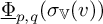 and
$\underline {\Phi }_{p,q}(\sigma _{\mathbb {W}}(w))$
 as differential forms on
$\partial \overline {B} \cong K/M$
 coincide along any smooth curve on
$\overline {B}$
 emanating from o. Under the identification of
$\mathcal {H}_{p,q}$
 with
$\Lambda ^{p,q}_0 H^*$
 these limits are given by
$\gamma _{p,q} \sigma _{\mathbb {V}}(v)(o)$
 using the formula from Proposition 21 and
$\frac {c_{p,q}\gamma _{p-1,q}}{n+1-k} \sigma _{\mathbb {W}}(w)(o)$
 via the formula in (ii), respectively. Arguing similarly for
$\mathbb {W} \in \hat {K}$
 satisfying the assumptions in (iii), it follows that the coefficients
$\gamma _{p,q}$
 satisfy the relations

which in turn characterize these numbers up to an overall constant. But (13) shows that
$\lambda _{p,q}^{-1}$
 also satisfy these relations, from which the claim follows.
The previous theorem also yields a description of the decomposition of the image of
$\underline {\Phi }_{p,q}$
 for
$p+q = n$
 into
$(p,q)$
 -types, which we state explicitly for later use.
Corollary 23. For
$0 \le p, q \le n$
 with
$p+q = n$
 let
$\mathcal {L}_{\pm } \subseteq \Gamma (\mathcal {H}_{p,q})$
 be the eigenspaces of
$\mathcal {L}_{\zeta }$
 with eigenvalues in
$\pm i\mathbb {R}$
 and define the subspaces
$\mathcal {K}$
 ,
$\mathcal {I}_1$
 and
$\mathcal {I}_2$
 of
$\Gamma (\mathcal {H}_{p,q})$
 via

For
$\mathbb {V} \in \hat {K}$
 and a K-invariant subspace
$A \subset \Gamma (\mathcal {H}_{p,q})$
 define
$A^{\mathbb {V}} := A \cap \Gamma (\mathcal {H}_{p,q})_{\mathbb {V}}$
 . Then

for all irreducible K-representations
$\mathbb {V}$
 .
Remark. By adjointness it follows that
$\Gamma (\mathcal {H}_{p,q})$
 decomposes naturally into the direct sum of the kernel of
$\mathcal {D}^*$
 and its orthogonal complement, which are both closed subspaces, and similarly for its complex conjugate operator. Moreover, each K-finite subrepresentation of
$\Gamma (\mathcal {H}_{p,q})$
 decomposes into irreducibles, each of which must be contained in one of the subspaces
$\mathcal {K}$
 ,
$\mathcal {I}_1$
 and
$\mathcal {I}_2$
 due to irreducibility. This shows that Theorem 22 yields a full description of
$d\underline {\Phi }_{p,q}(\Gamma (\mathcal {H}_{p,q}))$
 since K-finite vectors form a dense subspace.
5.3 The
$L^2$
-norm of
$d\underline{\Phi }{}_{p,q}$
on isotypic components


In the next step we use the explicit formulae for the image of
$\underline {\Phi }_{p,q}$
 on isotypic components from Theorem 22 to prove that
$d\underline {\Phi }_{p,q}(\alpha )$
 has finite
$L^2$
 -norm for all
$\alpha \in \Gamma (\mathcal {H}_{p,q})_{\mathbb {V}}$
 with
$p+q = n$
 . We do this by first showing that
$\underline {\Phi }_{p,q}(\alpha ) \in \Omega ^{p,q}(G/K)$
 as well as its exterior derivative are sufficiently bounded on
$\overline {B}$
 , which allows the application of Stokes’ theorem.
Proposition 24. For all
$\alpha \in \Gamma (\mathcal {H}_{p,q})_{\mathbb {V}}$
 with
$p+q=n$
 , the differential form
$\underline {\Phi }_{p,q}(\alpha ) \in \Omega ^{n}(B, \mathbb {C})$
 is smooth up to the boundary, whereas
$d\underline {\Phi }_{p,q}(\alpha ) = \phi _1 + f(r)\tau \wedge \overline {\tau } \wedge \phi _2$
 for
$f \in L^1([0,1])$
 and
$\phi _1, \phi _2 \in \Omega ^*(\overline {B}, \mathbb {C})$
 . Moreover, the
$L^2$
 -inner product
$\langle \!\langle d\underline {\Phi }_{p,q}(\alpha ), d\underline {\Phi }_{p,q}(\beta )\rangle \!\rangle $
 is finite for all
$\alpha $
 ,
$\beta \in \Gamma (\mathcal {H}_{p,q})_{\mathbb {V}}$
 . In particular,
$d\underline {\Phi }_{p,q}(\alpha )$
 is an
$L^2$
 -harmonic differential form.
Proof. The pullback of a differential form on
$S^{2n+1}$
 along the angular map
$\chi $
 as well as the differential forms
$\tau $
 and
$\overline {\tau }$
 are smoothly defined on
$\overline {B} \setminus \{0\}$
 . Thus, Theorem 22 implies that the restrictions to
$B \setminus \{0\}$
 of both
$\underline {\Phi }_{p,q}(\alpha )$
 and its exterior derivative are linear combinations of elements of the form
$f(r)\phi $
 , where
$\phi \in \Omega ^*(\overline {B}\setminus \{0\}, \mathbb {C})$
 and
$f \colon (0,1) \to \mathbb {C}$
 is a smooth function in the radial variable whose limit for
$r \to 0$
 exists. Moreover, each such f is a linear combination of
$F_{k,\lambda ,\mu }$
 for
$k \in \{n, n-1\}$
 as well as their first and second derivatives, and the latter can only appear in the coefficient of an element of the form
$\tau \wedge \overline {\tau } \wedge \phi $
 . Using the analytic properties of the hypergeometric function from Proposition 15, we have seen that the functions
$F_{k,\lambda ,\mu }$
 as well as their first derivatives can be smoothly extended to
$[0,1]$
 , whereas
$F_{n-1,\lambda , \mu }" \in L^1([0,1])$
 . From this the claims on
$\underline {\Phi }_{p,q}(\alpha )$
 and
$d\underline {\Phi }_{p,q}(\alpha )$
 follow.
For the computation of the
$L^2$
 -inner product recall from Proposition 11 that
$\underline {\Phi }_{p,q}(\alpha )$
 and
$\underline {\Phi }_{p,q}(\beta )$
 are harmonic and coclosed differential forms, which implies

Since
$\ast $
 is tensorial, it follows that the integrand of (23) can be written as
$d\psi _1 + g(r) d(\tau \wedge \overline {\tau }\wedge \psi _2)$
 with
$g \in L^1([0,1])$
 and
$\psi _1$
 ,
$\psi _2 \in \Omega ^*(\overline {B}, \mathbb {C})$
 . Now using a smooth approximation of g with support in B together with Stokes’ theorem, an easy estimate yields that the integral of the second summand is trivial. Thus, we can apply Stokes’ theorem to (23), and the domain of the resulting integral is the compact space
$\partial B \cong K/M$
 , showing that the
$L^2$
 -inner product is finite.
Remark. The above realization of
$L^2$
 -harmonic
$(n+1)$
 -forms also includes the construction given in [Reference Julg and Kasparov17, Theorem 3.2]. There, the initial data was a differential form
$\omega \in \Omega ^{p,q}(\mathbb {C}^{n+1})$
 with
$p+q = n+1$
 and p,
$q \neq 0$
 which is closed and primitive for the Euclidean metric. Furthermore, it was assumed that the coefficients of
$\omega $
 are homogeneous polynomials in z and
$\overline {z}$
 of degree k and m, respectively. To translate this to our setting, we view
$\omega $
 as an element of the irreducible K-representation
$\mathbb {V} := S^{k,m}(\mathbb {C})\otimes \Lambda ^{p,q}_0\mathbb {C}^{n+1}$
 , where
$S^{k,m}(\mathbb {C})$
 is the space of harmonic polynomials in z and
$\overline {z}$
 of degree k and m, respectively. Then
$\omega \mapsto \iota _{\overline {T}}\iota _T\omega |_{K/M}$
 defines a K-homomorphism
$\sigma \in \operatorname {\mathrm {Hom}}_K(\mathbb {V}, \Gamma (\mathcal {H}_{p-1,q-1}))$
 . Putting
$a := k + p$
 and
$b := m + q$
 , the formula for
$\Delta _H$
 in [Reference Rumin27, Proposition 2] yields that
$\mathcal {L}_{\zeta }\sigma = i(a-b)\sigma $
 and
$\Delta _H\sigma = (a+b+2ab)\sigma $
 , and inserting this into Proposition 21 shows that
$\underline {\Phi }_{p-1,q-1}(\sigma (\omega )) = cF(1)^{-1} r^{a+b}F(t)\chi ^*\sigma (\omega )$
 with
$F(t) := {}_2F_1(a,b,a+b+2;t)$
 . The differential forms
$\overline {\partial }(F(t)\sigma (\omega ))$
 and
$-\partial (F(t)\sigma (\omega ))$
 coincide with the forms
$\varphi _T$
 and
$\varphi _{\overline {T}}$
 in [Reference Julg and Kasparov17], and thus
$\underline {\Phi }_{p-1,q-1}(\sigma (\omega ))$
 coincides with the formula in the paper up to normalization with
$F(1)^{-1}$
 and the factor
$r^{a+b}$
 , the latter appearing due to the pullback along the angular map.
Although the previous proposition guarantees that the image of
$d\underline {\Phi }_{p,q}$
 on each isotypic component of
$\Gamma (\mathcal {H}_{p,q})$
 consists of
$L^2$
 -harmonic forms on
$G/K$
 , this is not sufficient to show the same property for the image of
$d\underline {\Phi }_{p,q}$
 on all of
$\Gamma (\mathcal {H}_{p,q})$
 . Therefore, we aim to express the
$L^2$
 -norm of
$d\underline {\Phi }_{p,q}(\alpha )$
 in terms of globally defined operators on
$K/M$
 , which then can be extended to all of
$\Gamma (\mathcal {H}_{p,q})$
 . It turns out that a slight variation of the
$L^2$
 -inner product gives a nicer description in terms of boundary operators. Explicitly, from [Reference Weil28, Theorem 1.3] we know that the Hodge star operator acts on primitive
$(n+1)$
 -forms on
$G/K$
 by multiplication with a non-zero number, which implies that

coincides with the
$L^2$
 -inner product of
$d\underline {\Phi }_{p,q}(\alpha )$
 and
$d\underline {\Phi }_{p,q}(\beta )$
 up to a multiple and is therefore finite. Our aim is to relate this expression to the
$(n+1)$
 -st BGG-operator, for which we use the following formula.
Lemma 25. Let
$0 \le p, q \le n$
 with
$p+q = n$
 , let
$\mathbb {V} \in \widehat {K}$
 and
$\alpha $
 ,
$\beta \in \Gamma (\mathcal {H}_{p,q})_{\mathbb {V}}$
 . Then we can write

with smooth functions
$f_1$
 ,
$f_2 \colon (0,1) \to \mathbb {C}$
 whose limits for
$r \to 1$
 exist. Furthermore,

where
$\vartheta \in \Omega ^1(K/M)$
 denotes the contact form.
Proof. The integrand on the left hand side of (24) can be written as the exterior derivative of
$\Psi := \underline {\Phi }_{p,q}(\alpha ) \wedge \overline {d\underline {\Phi }_{p,q}(\beta )} \in \Omega ^{2n+1}(\overline {B}, \mathbb {C})$
 . Therefore, its wedge product with
$\tau \wedge \overline {\tau }$
 has to be trivial, and thus Proposition 24 implies that modulo
$\tau \wedge \overline {\tau }$
 we can write
$\Psi $
 as a linear combination of
$\tau \wedge \psi _1$
 and
$\overline {\tau } \wedge \psi _2$
 , where
$\psi _1$
 ,
$\psi _2 \in \Omega ^{n,n}(G/K)$
 are trivial upon insertion of either vector field T,
$\overline {T} \in \mathfrak {X}(G/K)$
 . In particular, for fixed
$r \in (0,1)$
 we can use the angular map to identify the restriction of
$\psi _j$
 to the r-sphere
$S_r$
 of B with a section of
$\Lambda ^{n,n} H^*$
 . But the latter bundle has rank
$1$
 , implying that we can write
$\psi _j = f_j(r) \chi ^*(\alpha \wedge \overline {\beta })$
 . Therefore,
$\Psi $
 has the claimed form, and the limits of the coefficient functions exist due to Proposition 24. For the integral we write the left hand side of (24) as the integral over
$d\Psi $
 , and as in the proof of Proposition 24, the component of
$\Psi $
 containing
$\tau \wedge \overline {\tau }$
 does not contribute to this integral. Thus, the formula follows from Stokes’ theorem and the fact that the inclusion
$\iota \colon K/M \hookrightarrow \overline {B}$
 satisfies
$\iota ^*\tau = i \vartheta $
 .
We will use the lemma to relate the left hand side of (24) to an integral over
$K/M$
 involving the
$(n+1)$
 -st BGG-operator. In order to do so, recall that for
$0 \le p, q\le n$
 with
$p+q = n$
 the invariant operator
$\underline {D}_{n+1}$
 on
$\Gamma (\mathcal {H}_{p,q})$
 is the component of
$\iota _{\zeta }D_{n+1}$
 preserving the bidegree. By the multiplicity
$1$
 property from Proposition 18 this operator acts by a scalar
$\nu \in i\mathbb {R}$
 on each
$\mathbb {V}$
 -isotypic component of
$\Gamma (\mathcal {H}_{p,q})$
 , and we computed this factor explicitly in Corollary 20.
Theorem 26. For
$0 \le p, q \le n$
 with
$p+q = n$
 and
$\mathbb {V} \in \widehat {K}$
 let
$\alpha $
 ,
$\beta \in \Gamma (\mathcal {H}_{p,q})_{\mathbb {V}}$
 . Let
$\lambda _{p,q} \in \mathbb {C}$
 be the coefficients in the definition of
$\underline {\Phi }_{n}$
 from Theorem 12 and let
$c\in \mathbb {C}$
 be the constant from Theorem 22 (which is independent of
$\mathbb {V}$
 , p and q). Then we have

Equivalently, if
$\nu $
 is the eigenvalue of
$\underline {D}_{n+1}$
 on
$\Gamma (\mathcal {H}_{p,q})_{\mathbb {V}}$
 , then

Proof. By comparing bidegrees we can replace
$D_{n+1}\overline {\beta }$
 by
$\vartheta \wedge \underline {D}_{n+1}\overline {\beta }$
 on the right hand side of (25). Since
$\nu \in i\mathbb {R}$
 is purely imaginary, complex conjugation yields
$\underline {D}_{n+1}\overline {\beta } = -\nu \overline {\beta }$
 . Therefore, if
$f_1(r)$
 and
$f_2(r)$
 are as in Lemma 25, it suffices to prove

for the constant
$c \in \mathbb {C}$
 coming from the explicit formulae for the image of
$\underline {\Phi }_{p,q}$
 on isotypic components in Theorem 22. In order to do so, let
$\lambda $
 and
$\mu $
 be the eigenvalues of
$\mathcal {L}_{\zeta }$
 and
$\Delta _H$
 on
$\Gamma (\mathcal {H}_{p,q})_{\mathbb {V}}$
 , respectively, and write
$\alpha = \sigma (v)$
 and
$\beta =\sigma (w)$
 for v,
$w \in \mathbb {V}$
 and
$\sigma \in \operatorname {\mathrm {Hom}}_K(\mathbb {V}, \Gamma (\mathcal {H}_{p,q}))$
 , which is unique up to multiples.
(i) If
$\sigma (\mathbb {V}) \subseteq \operatorname {\mathrm {im}}(\mathcal {D}^*) \cap \operatorname {\mathrm {im}}(\overline {\mathcal {D}}^*)$
 , then since
$\underline {\Phi }_{p,q} \circ \mathcal {D}$
 is a nontrivial multiple of
$\partial \circ \underline {\Phi }_{p-1,q}$
 as well as for their complex conjugates due to Theorem 6 we obtain
$d\underline {\Phi }_{p,q}\beta = 0$
 , whereas
$D_{n+1}\overline {\beta } = 0$
 due to Corollary 20(iv).
(ii) If
$\sigma (\mathbb {V}) \subseteq \ker (\mathcal {D}^*) \cap \ker (\overline {\mathcal {D}}^*)$
 , then
$\underline {\Phi }_{p,q}(\alpha ) = \lambda _{p,q}^{-1} cr^{|\lambda |}\chi ^*\alpha $
 and
$\nu = \lambda $
 . Since
$\partial _H\beta = 0$
 and
$\overline {\partial }_H\beta = 0$
 due to Proposition 19(iv), the exterior derivative of
$\underline {\Phi }_{p,q}(\beta )$
 is a linear combination of
$\tau \wedge \chi ^*\beta $
 and
$\overline {\tau } \wedge \chi ^*\beta $
 , and determining the coefficients explicitly yields (26).
(iii) If
$\sigma (\mathbb {V}) \cap \ker (\mathcal {D}^*) = \{0\}$
 and
$\sigma (\mathbb {V}) \subset \ker (\overline {\mathcal {D}}^*)$
 , then we have
$\underline {\Phi }_{p,q}(\alpha ) = 2 \lambda _{p,q}^{-1}c\mu ^{-1} \partial (f(r) \chi ^*\partial _H^*\alpha )$
 with
$f(r) = F_{n-1, \lambda , \mu +i\lambda }(1)^{-1}F_{n-1,\lambda , \mu +i\lambda }(r)$
 , whereas
$\nu = \lambda - \frac {i}{2}\mu $
 . Define the functions
$g_{\pm }(r) := \frac {1}{2r} (f' \pm i\lambda f)$
 and note that since
$f'(1) = \mu + i\lambda $
 due to (21), we get
$g_-(1) = \frac {\mu }{2}$
 and
$g_+(1) = \frac {\mu }{2} + i\lambda $
 . Moreover, a few lines of computation using the calculus on
$K/M$
 and B from Propositions 8 and 13 yield that, modulo
$\tau \wedge \overline {\tau }$
 , we get

Since formula (24) in Lemma 25 only depends on the values of the functions
$f_1$
 and
$f_2$
 at
$r = 1$
 , we can omit all summands in
$\overline {\partial }\underline {\Phi }_{p,q}(\beta )$
 whose boundary value is trivial. A direct computation shows that this is the case for the coefficient function of
$\chi ^*\overline {\partial }_H\beta $
 . Moreover,
$\overline {\partial }_H\partial _H^*\beta $
 has values in
$\mathcal {H}_{p-1,q+1}$
 and thus the wedge product of its complex conjugate with
$\underline {\Phi }_{p,q}(\alpha )$
 is trivial. Therefore, we can replace
$\overline {\partial }\underline {\Phi }_{p,q}(\beta )$
 with
$g_+ \overline {\tau } \wedge \chi ^*\beta $
 , and a direct computation shows that
$f_2(1) = 0$
 and
$f_1(1) = (-1)^n\lambda _{p,q}^{-1} |c|^2(\frac {\mu }{2} + i \lambda )$
 , proving (26).
(iv) The case
$\sigma (\mathbb {V}) \subseteq \ker (\mathcal {D}^*)$
 and
$\sigma (\mathbb {V}) \cap \ker (\overline {\mathcal {D}}^*) = \{0\}$
 follows from (iii) since
$\underline {\Phi }_{p,q}$
 is compatible with complex conjugation due to Theorem 6.
To prove the last statement, we use that the Hodge star operator acts on a primitive
$(s,t)$
 -form on
$G/K$
 with
$s+t = n+1$
 by multiplication with
$(-1)^{\frac {(n+1)(n+2)}{2}} i^{s-t}$
 due to [Reference Weil28, Theorem 1.3], and a similar proof yields that the Hodge star operator
$\ast _H$
 acts on primitive sections of
$\Lambda ^{p,q} H^*$
 with
$p+q = n$
 by multiplication with
$(-1)^{\frac {n(n+1)}{2}} i^{p-q}$
 . Now from Theorem 22 we know that
$\underline {\Phi }_{p,q}(\beta )$
 is in the kernel of
$\partial $
 or
$\overline {\partial }$
 , and the rest follows from an easy computation.
6 Poisson transforms and discrete series representations
As a last step, we analyze the real operator
$\underline {\Phi }_n \colon \Gamma (\mathcal {H}_n) \to \Omega ^n(G/K)$
 defined in Theorem 12 to prove that the image of
$d\underline {\Phi }_n$
 consists of
$L^2$
 -forms. Now it is well known, see [Reference Pedon26], that the space
$L^2\Omega ^{n+1}_{\Delta }(G/K)$
 of
$L^2$
 -harmonic
$(n+1)$
 -forms on
$G/K$
 is a realization of the direct sum of all discrete series representations of G with trivial infinitesimal character. Recall that a discrete series representation for a linear connected semisimple Lie group G is an irreducible representation on a Hilbert space
$\mathcal {H}$
 so that its matrix coefficients are contained in
$L^2(G)$
 . By [Reference Knapp19, Theorem 12.20] such representations can only exist if the ranks of G and its maximal compact subgroup K coincide. Furthermore, if this is the case, then the number of inequivalent discrete series representations with the same infinitesimal character equals
$|W_G|/|W_K|$
 , where
$W_G$
 and
$W_K$
 are the Weyl groups of G and K, respectively. Now in [Reference Borel4, Theorem A] it was shown that discrete series representations with trivial infinitesimal character can be realized as
$L^2$
 -harmonic differential forms on
$G/K$
 , which can only exist in degree
$\frac {1}{2} \dim _{\mathbb {R}}(G/K)$
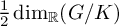 . In our setting we have
$|W_G|/|W_K| = n+2$
 , and it was computed in [Reference Borel and Wallach5, Theorem 4.11] and [Reference Pedon26, Theorem 3.4] that the inequivalent discrete series representations with trivial infinitesimal character correspond to the decomposition of
$L^2$
 -harmonic
$(n+1)$
 -forms into
$(p,q)$
 -types.
6.1 The image of
$d \underline { \Phi }_n$
on K-finite vectors

Recall from Theorem 12 that the real operator
$\underline {\Phi }_n \colon \Gamma (\mathcal {H}_n) \to \Omega ^n(G/K)$
 was defined as a linear combination of the complex operators
$\underline {\Phi }_{p,q} \colon \Gamma (\mathcal {H}_{p,q}) \to \Omega ^{p,q}(G/K)$
 . Moreover, the space of K-finite vectors of
$\Gamma (\mathcal {H}_n)$
 is a dense subspace which decomposes into the sum of isotypic components. Thus, in order to gain information about the kernel and the image of
$d\underline {\Phi }_n$
 , we will first consider its restriction to isotypic components and apply the results from Sections 5.2 and 5.3, and afterwards use a completion argument to obtain general results.
Given a K-finite section
$\alpha \in \Gamma (\mathcal {H}_n)$
 , we can first decompose it into
$(p,q)$
 -types
$\alpha _{p,q}$
 and afterwards into isotypic components
$\alpha _{p,q}^{\mathbb {V}}$
 . Since the projection
$\mathcal {H}_n \to \mathcal {H}_{p,q}$
 is K-equivariant and tensorial, it follows that
$\Gamma (\mathcal {H}_n)_{\mathbb {V}} \cap \Gamma (\mathcal {H}_{p,q})$
 coincides with the
$\mathbb {V}$
 -isotypic component
$\Gamma (\mathcal {H}_{p,q})_{\mathbb {V}}$
 . In particular, we can write each element in
$\Gamma (\mathcal {H}_n)_{\mathbb {V}}$
 as a sum of elements in
$\Gamma (\mathcal {H}_{p,q})_{\mathbb {V}}$
 . Since different isotypic components and
$(p,q)$
 -types are orthogonal, it follows that
$\alpha = 0$
 if and only if
$\alpha ^{\mathbb {V}}_{p,q} = 0$
 for all
$\mathbb {V} \in \widehat {K}$
 and all
$0 \le p, q \le n$
 with
$p+q = n$
 . Similarly, if
$\beta \in \Gamma (\mathcal {H}_n)$
 is a K-finite section, then using K-invariance of the
$L^2$
 -inner product, it follows that
$\langle \!\langle \alpha , \beta \rangle \!\rangle $
 coincides with the sum of
$\langle \!\langle \alpha ^{\mathbb {V}}_{p,q}, \beta ^{\mathbb {V}}_{p,q} \rangle \!\rangle $
 over all
$\mathbb {V} \in \hat {K}$
 and
$p+q = n$
 .
Next, the space
$\Omega ^{n+1}(G/K)$
 is naturally a unitary K-representation, and since
$d\underline {\Phi }_n$
 is K-equivariant, it maps
$\mathbb {V}$
 -isotypic components to
$\mathbb {V}$
 -isotypic components. Thus, by linearity of
$d\underline {\Phi }_n$
 it follows that
$d\underline {\Phi }_n(\alpha ) = 0$
 if and only if
$d\underline {\Phi }_n(\alpha ^{\mathbb {V}}) = 0$
 for all
$\mathbb {V} \in \hat {K}$
 . Furthermore, for the
$L^2$
 -inner product we obtain that
$\langle \!\langle d\underline {\Phi }_n(\alpha ), d\underline {\Phi }_n(\beta )\rangle \!\rangle $
 is the sum of
$\langle \!\langle d\underline {\Phi }_n(\alpha ^{\mathbb {V}}) , d\underline {\Phi }_n(\beta ^{\mathbb {V}})\rangle \!\rangle $
 over all
$\mathbb {V} \in \hat {K}$
 . However, since
$d\underline {\Phi }_n$
 does not preserve the bidegree, it follows that the differential forms
$d\underline {\Phi }_n(\alpha _{p,q})$
 can be linearly dependent for different values of p and q. In the following lemma we show that this only happens in one specific situation.
Lemma 27. For
$\mathbb {V} \in {\hat {K}}$
 and
$1 \le s,t \le n$
 with
$s+t = n+1$
 let
$\alpha _{s-1,t} \in \Gamma (\mathcal {H}_{s-1,t})_{\mathbb {V}}$
 and
$\alpha _{s,t-1} \in \Gamma (\mathcal {H}_{s,t-1})_{\mathbb {V}}$
 and assume that both
$\partial \underline {\Phi }_n(\alpha _{s-1,t})$
 and
$\overline {\partial } \underline {\Phi }_n(\alpha _{s,t-1})$
 are nontrivial. Then
$\alpha _{s-1,t} \in \ker (\mathcal {D}^*)$
 and
$\alpha _{s,t-1} \in \ker (\overline {\mathcal {D}}^*)$
 . Moreover, we have one of two possible cases:
-
(i) The elements $\alpha _{s-1,t}$
and
$\alpha _{s,t-1}$
are contained in the kernels of both
$\mathcal {D}^*$
and
$\overline {\mathcal {D}}^*$
. Moreover,
$\partial \underline {\Phi }_n(\alpha _{s-1,t})$
and
$\overline {\partial } \underline {\Phi }_n(\alpha _{s,t-1})$
are orthogonal with respect to the
$L^2$
-inner product. -
(ii) We have $\alpha _{s-1,t} \in \operatorname {\mathrm {im}}(\overline {\mathcal {D}})$
as well as
$\alpha _{s,t-1} \in \operatorname {\mathrm {im}}(\mathcal {D})$
, and we can write $$ \begin{align*} \partial \underline{\Phi}_n(\alpha_{s-1,t}) + \overline{\partial} \underline{\Phi}_n(\alpha_{s,t-1}) = \partial\overline{\partial} \underline{\Phi}_{n-1}({\hat{\alpha}}_1- {\hat{\alpha}}_2) \end{align*} $$for ${\hat {\alpha }}_j \in \Gamma (\mathcal {H}_{s-1,t-1})_{\mathbb {V}}$
with
$\alpha _{s-1,t} = \overline {\mathcal {D}} {\hat {\alpha }}_1$
and
$\alpha _{s,t-1} = \mathcal {D}{\hat {\alpha }}_2$
.


Proof. Let
$\sigma _{p,q} \in \operatorname {\mathrm {Hom}}_K(\mathbb {V}, \Gamma (\mathcal {H}_{p,q}))$
 so that
$\alpha _{p,q} \in \operatorname {\mathrm {im}}(\sigma _{p,q})$
 . By the multiplicity
$1$
 property in Proposition 18 we know that
$\sigma _{p,q}$
 is unique up to multiples, and by assumption both
$\sigma _{s-1,t}$
 and
$\sigma _{s,t-1}$
 are non-zero. From Corollary 23 it follows that
$\partial \underline {\Phi }_n(\alpha _{s-1,t}) \neq 0$
 only if
$\alpha _{s-1,t} \in \ker (\mathcal {D}^*)$
 , which by irreducibility of
$\mathbb {V}$
 is equivalent to
$\sigma _{s-1,t}(\mathbb {V}) \subseteq \ker (\mathcal {D}^*)$
 , and similarly for
$\overline {\partial } \underline {\Phi }_n(\alpha _{s,t-1})$
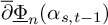 . Furthermore, by irreducibility of
$\mathbb {V}$
 it follows that
$\sigma _{s-1,t}(\mathbb {V})$
 is either a subspace of
$\ker (\overline {\mathcal {D}}^*)$
 or has trivial intersection with it.
If
$\sigma _{s-1,t}(\mathbb {V}) \cap \ker (\overline {\mathcal {D}}^*) = \{0\}$
 , then we can write
$\sigma _{s-1,t} = \overline {\mathcal {D}}\hat {\sigma }$
 for
${\hat {\sigma }} \in $
 $\operatorname {\mathrm {Hom}}_K(\mathbb {V}, \Gamma (\mathcal {H}_{s-1,t-1}))$
 . Since
$\alpha _{s-1,t} = \sigma _{s-1,t}(v)$
 for
$v \in \mathbb {V}$
 , this shows that
$\alpha _{s-1,t} \in \operatorname {\mathrm {im}}(\overline {\mathcal {D}})$
 . Furthermore,
$\mathcal {D}\hat {\sigma } \neq 0$
 , because otherwise we have

contradicting our assumption. By the multiplicity
$1$
 property in Proposition 18, the map
$\mathcal {D}\hat {\sigma }$
 has to be a nontrivial multiple of
$\sigma _{s,t-1}$
 , which shows that
$\alpha _{s,t-1} \in \operatorname {\mathrm {im}}(\mathcal {D})$
 . Moreover, by adjointness this implies
$\mathcal {D}^*\sigma _{s,t-1} \neq 0$
 and therefore
$\sigma _{s,t-1}(\mathbb {V}) \cap \ker (\mathcal {D}^*) = \{0\}$
 . Additionally, from Theorem 12 we know that
$\underline {\Phi }_n \circ D_n = d \circ \underline {\Phi }_{n-1}$
 , which implies the claim for the sum of the derivatives. Via an analogous argument we also obtain that
$\sigma _{s-1,t}(\mathbb {V}) \cap \ker (\overline {\mathcal {D}}^*) = \{0\}$
 is equivalent to
$\sigma _{s,t-1}(\mathbb {V}) \cap \ker (\mathcal {D}^*) = \{0\}$
 , proving that we are always in one of the two claimed cases.
In the other case,
$\sigma _{s-1,t}(\mathbb {V})$
 and
$\sigma _{s,t-1}(\mathbb {V})$
 are contained in the kernels of both
$\mathcal {D}^*$
 and
$\overline {\mathcal {D}}^*$
 . Moreover, we have seen in the proof of Theorem 26 that
$\partial \underline {\Phi }_n(\alpha _{s-1,t})$
 and
$\overline {\partial } \underline {\Phi }_n(\alpha _{s,t-1})$
 are multiples of
$\tau \wedge \chi ^*\alpha _{s-1,t}$
 and
$\overline {\tau } \wedge \chi ^*\alpha _{s,t-1}$
 , respectively, which are orthogonal with respect to the
$L^2$
 -inner product.
Now we have all ingredients at hand to prove the main result of this article, which explicitly relates the BGG complex to the discrete series representations of G.
Theorem 28. Let
$G = \operatorname {\mathrm {SU}}(n+1,1)$
 ,
$K \subset G$
 its maximal compact subgroup and
$P \subset G$
 its minimal parabolic subgroup, and consider the G-equivariant operator
$\underline {\Phi }_n \colon \Gamma (\mathcal {H}_n) \to \Omega ^n(G/K)$
 from Theorem 12.
-
(i) We have $\ker (d\underline {\Phi }_n) = \operatorname {\mathrm {im}}(D_{n})$
, where
$D_{n}$
is the n-th BGG-operator. -
(ii) For all $\alpha $
,
$\beta \in \Gamma (\mathcal {H}_n)$
we have (27) $$ \begin{align} \int_{G/K} d\underline{\Phi}_n(\alpha) \wedge d\underline{\Phi}_n(\overline{\beta}) = |c|^2\int_{G/P} \alpha \wedge D_{n+1}\overline{\beta} \end{align} $$for the constant $c \in \mathbb {C}$
from Theorem 22. In particular,
$\langle \!\langle d\underline {\Phi }_n(\alpha ), d\underline {\Phi }_n(\beta ) \rangle \!\rangle $
is finite, and the differential form
$d\underline {\Phi }_n(\alpha ) \in \Omega ^{n+1}(G/K)$
is
$L^2$
-harmonic.
-
(iii) The Poisson transform $d\underline {\Phi }_n$
maps
$\Gamma (\mathcal {H}_n)/\operatorname {\mathrm {im}}(D_{n})$
isomorphically onto a dense subspace of the space
$L^2\Omega ^{n+1}_{\Delta }(G/K)$
of
$L^2$
-harmonic
$(n+1)$
-forms on
$G/K$
, which is the direct sum of all discrete series representations of G with trivial infinitesimal character.


Proof. (i) By Theorem 12 we have
$\underline {\Phi }_n \circ D_n = d \circ \underline {\Phi }_{n-1}$
 and thus
$\operatorname {\mathrm {im}}(D_n) \subseteq \ker (d\underline {\Phi }_n)$
 . For the other direction note that both
$\ker (d\underline {\Phi }_n)$
 and
$\operatorname {\mathrm {im}}(D_n) = \ker (D_{n+1})$
 are closed K-invariant subspaces of
$\Gamma (\mathcal {H}_n)$
 . Moreover, the subspace of K-finite vectors
$\ker (d\underline {\Phi }_n)^{fin}$
 of
$\ker (d\underline {\Phi }_n)$
 is dense. Therefore, if
$\ker (d\underline {\Phi }_n)$
 is contained in
$\operatorname {\mathrm {im}}(D_n)$
 , then taking the closure of the chain of inclusions
$\ker (d\underline {\Phi }_n)^{fin} \subseteq \operatorname {\mathrm {im}}(D_n) \subseteq \ker (d\underline {\Phi }_n)$
 implies the claim. Furthermore, we have seen that for a K-finite section
$\alpha \in \Gamma (\mathcal {H}_n)$
 we have
$d\underline {\Phi }_n(\alpha ) = 0$
 if and only if
$d\underline {\Phi }_n$
 is trivial on each isotypic component of
$\alpha $
 .
Therefore, for a fixed
$\mathbb {V} \in \hat {K}$
 , let
$\alpha \in \Gamma (\mathcal {H}_n)_{\mathbb {V}}$
 with
$d\underline {\Phi }_n(\alpha ) = 0$
 and let
$\alpha = \sum _{p+q=n} \alpha _{p,q}$
 be its decomposition into
$(p,q)$
 -types. From Corollary 23 it follows that
$\underline {\Phi }_n(\alpha _{p,q})$
 is contained in
$\ker (\partial )$
 or in
$\ker (\overline {\partial })$
 , and
$d\underline {\Phi }_n(\alpha _{p,q}) = 0$
 if and only if
$\alpha _{p,q} \in \ker (\mathcal {D}^*)^{\perp } \cap \ker (\overline {\mathcal {D}}^*)^{\perp }$
 . Writing
$\alpha _{p,q} = \sigma _{p,q}(v)$
 with
$\sigma _{p,q} \in \operatorname {\mathrm {Hom}}_K(\mathbb {V}, \Gamma (\mathcal {H}_{p,q}))$
 this means that
$\sigma _{p,q}(\mathbb {V}) \cap \ker (\mathcal {D}^*) = \{0\}$
 and
$\sigma _{p,q}(\mathbb {V}) \cap \ker (\overline {\mathcal {D}}^*) = \{0\}$
 , and by Corollary 20 this implies that
$D_{n+1} \circ \sigma _{p,q} = 0$
 and thus
$\alpha _{p,q} \in \ker (D_{n+1}) = \operatorname {\mathrm {im}}(D_n)$
 .
By symmetry we can assume w.l.o.g that
$\partial \underline {\Phi }_n(\alpha _{s-1,t}) \neq 0$
 for indices
$0 \le s, t \le n+1$
 with
$s+t = n+1$
 . Since
$d\underline {\Phi }_n(\alpha ) = 0$
 , this implies
$\partial \underline {\Phi }_n(\alpha _{s-1,t}) = -\overline {\partial } \underline {\Phi }_n(\alpha _{s,t-1})$
 by comparing
$(p,q)$
 -types. From Lemma 27 we know that this is only possible if
$\alpha _{s-1,t} = \overline {\mathcal {D}} \hat {\alpha }_1$
 and
$\alpha _{s,t-1} = \mathcal {D} \hat {\alpha }_2$
 for
$\hat {\alpha }_j \in \Gamma (\mathcal {H}_{s-1,t-1})_{\mathbb {V}}$
 , and we obtain the relation
$\partial \overline {\partial }\underline {\Phi }_{n-1}(\hat {\alpha }_1) = \partial \overline {\partial }\underline {\Phi }_{n-1}(\hat {\alpha }_2)$
 . From the explicit formulae for the image of the Poisson transform on the Poincaré ball model in Theorem 22 this is only possible if
$\hat {\alpha }_1 = \hat {\alpha }_2$
 and thus
$\alpha _{s-1,t} + \alpha _{s,t-1} \in \operatorname {\mathrm {im}}(D_n)$
 .
(ii) As in the proof of Theorem 26, we obtain that the left hand side of (27) is a nontrivial multiple of the
$L^2$
 -inner product on
$G/K$
 , whereas the right hand side can be written as a multiple of
$\langle \!\langle \alpha , \iota _{\zeta }D_{n+1}\beta \rangle \!\rangle $
 . Now assume that we have shown the claimed equation for all K-finite vectors
$\alpha $
 ,
$\beta \in \Gamma (\mathcal {H}_n)$
 . Then for fixed
$\beta $
 both sides of (27) are continuous functions
$\Gamma (\mathcal {H}_n) \to \mathbb {R}$
 which coincide on the dense subspace of K-finite vectors and thus have to be equal on all of
$\Gamma (\mathcal {H}_n)$
 . Now for fixed
$\alpha \in \Gamma (\mathcal {H}_n)$
 the same argument shows equality of (27) for all
$\beta \in \Gamma (\mathcal {H}_n)$
 . Moreover, isotypic components of
$\Gamma (\mathcal {H}_n)$
 are orthogonal, so since both operators
$d\underline {\Phi }_n$
 and
$D_{n+1}$
 are K-equivariant and linear, it suffices to prove equation (27) for elements in
$\Gamma (\mathcal {H}_n)_{\mathbb {V}}$
 . Furthermore, we can decompose
$\alpha $
 into
$(p,q)$
 -types and use linearity to expand both sides of equation (27). Then the claimed equation is true for
$\alpha $
 if and only if it is valid for
$\alpha _{p,q}$
 for all
$p+q = n$
 . Therefore, we fix
$0 \le p, q \le n$
 with
$p+q = n$
 and let
$\alpha \in \Gamma (\mathcal {H}_{p,q})_{\mathbb {V}}$
 and
$\beta \in \Gamma (\mathcal {H}_n)_{\mathbb {V}}$
 . Comparing the types of forms on the left and right hand sides of (27), it follows that in the decomposition of
$\beta $
 into
$(p,q)$
 -types only
$\beta _{p+1,q-1}$
 ,
$\beta _{p,q}$
 and
$\beta _{p-1,q+1}$
 can contribute nontrivially. Using linearity of
$d\underline {\Phi }_n$
 ,
$D_{n+1}$
 and the integral, it suffices to show the validity of the equation for these three cases. Moreover, for
$\beta _{p,q}$
 the claim was already proven in Theorem 26.
For
$\beta = \beta _{p+1,q-1} \neq 0$
 the left hand side of (27) reduces to the integral over the wedge product of
$\partial \underline {\Phi }_n(\alpha )$
 and
$\partial \underline {\Phi }_n(\overline {\beta }) $
 , whereas via the explicit formula for
$D_{n+1}$
 from Theorem 9, the right hand side is a multiple of
$\langle \!\langle \alpha , \overline {\partial }_H\partial _H^*\beta \rangle \!\rangle = \langle \!\langle \overline {\partial }_H^*\alpha , \partial _H^*\beta \rangle \!\rangle $
 . Now if
$\overline {\partial }\underline {\Phi }_n(\alpha ) = 0$
 , then by Corollary 23, we have
$\alpha \in \ker (\overline {\mathcal {D}}^*) = \ker (\overline {\partial }_H^*)$
 , showing that both sides of (27) are trivial. By symmetry the analogous statement is true if
$\partial \underline {\Phi }_n(\overline {\beta }) = 0$
 , so we can assume that
$\overline {\partial }\underline {\Phi }_n(\alpha )$
 and
$\partial \underline {\Phi }_n(\overline {\beta })$
 are both nontrivial. Now if we are in the first case of Lemma 27, i.e. if
$\alpha $
 and
$\beta $
 are both contained in
$\ker (\mathcal {D}^*) \cap \ker (\overline {\mathcal {D}}^*)$
 , then the exterior derivatives are orthogonal and thus the left hand side of (27) is trivial, whereas the right hand side is trivial since
$\partial _H^*\alpha = 0$
 . If we are in the second case of Lemma 27, we can write
$\beta = \mathcal {D} \gamma $
 with
$\gamma \in \Gamma (\mathcal {H}_{p, q-1})_{\mathbb {V}}$
 . Applying the relation
$\partial \circ \underline {\Phi }_{n-1} = \underline {\Phi }_n \circ \mathcal {D}$
 and anticommutativity of
$\partial $
 and
$\overline {\partial }$
 , we obtain
$\partial \underline {\Phi }_n(\overline {\beta }) = - \overline {\partial }\underline {\Phi }_n(\mathcal {D} \overline {\gamma })$
 , whereas
$D_{n+1}(\overline {\beta }) = - D_{n+1}(\mathcal {D} \overline {\gamma })$
 due to
$D_{n+1} \circ D_n = 0$
 . Since
$\mathcal {D}\gamma \in \Gamma (\mathcal {H}_{p,q})_{\mathbb {V}}$
 , equation (27) follows again from Theorem 26. In the case
$\beta = \beta _{p-1,q+1}$
 we can argue analogously.
(iii) By part (ii),
$d\underline {\Phi }_n$
 has values in
$L^2\Omega ^{n+1}_{\Delta }(G/K)$
 , and by part (i), it descends to
$\Gamma (\mathcal {H}_n)/\operatorname {\mathrm {im}}(D_n)$
 . Thus, we only have to show that the image of
$d\underline {\Phi }_n$
 is dense. For
$0 \le s, t \le n+1$
 with
$s+t = n+1$
 let
$\pi _{s,t} \colon \Omega ^{n+1}(G/K) \to \Omega ^{s,t}(G/K)$
 be the G-equivariant projection onto the
$(s,t)$
 -type. Since the Laplace operator is G-equivariant and preserves types, it follows that the image of a harmonic form on
$G/K$
 under
$\pi _{s,t}$
 is again harmonic. Similarly, the
$L^2$
 -inner product is G-invariant, and different
$(s,t)$
 -types are orthogonal, implying that
$\pi _{s,t}$
 maps between differential forms with finite
$L^2$
 -norm. Therefore, we obtain an induced map
$\pi _{s,t} \colon L^2\Omega ^{n+1}_{\Delta }(G/K) \to L^2\Omega ^{s,t}_{\Delta }(G/K)$
 , which is again G-equivariant. Combining this with
$d\underline {\Phi }_n$
 yields a continuous G-equivariant map
$\Gamma (\mathcal {H}_n)/\operatorname {\mathrm {im}}(D_n)\to L^2\Omega _{\Delta }^{s,t}(G/K)$
 , which is nontrivial. Now the target space is an irreducible G-module due to [Reference Pedon26, Theorem 3.4] and thus the image has to be dense.
Formula (27) explicitly describes the pullback of the
$L^2$
 -inner product on
$L^2\Omega ^{n+1}_{\Delta }(G/K)$
 to
$\Gamma (\mathcal {H}_n)$
 . Hence the direct sum of discrete series representations of G can be identified with the completion of
$\Gamma (\mathcal {H}_n)/\operatorname {\mathrm {im}}(D_{n-1})$
 with respect to this inner product. Now one can rewrite the right hand side of (27) in terms of the operator
$\sqrt {D_{n+1}^*D_{n+1}}$
 to arrive at a description parallel to the one obtained by J. Lott in [Reference Lott22] for the case of
$\operatorname {\mathrm {SO}}_0(n+1,1)$
 . This was used to identify the sum of discrete series representations of the latter group with a space of differential forms lying in the Sobolev space
$H^{-1/2}$
 .
Acknowledgements
We thank the anonymous referee for several comments that helped improving the paper.
Funding
The first and second authors were supported by the Austrian Science Fund (FWF): P 33559-N. This article is based on work from COST Action CaLISTA CA21109, supported by COST (European Cooperation in Science and Technology). https://www.cost.eu.
Competing interests
The authors declare none.
Data Availability Statement
Data availability is not applicable to this article as no new data were created or analyzed in this study.


 Open access

