
1. Introduction
The thermal resistance associated with the interface between two materials is of great fundamental as well as practical importance (Cahill et al. Reference Cahill, Ford, Goodson, Mahan, Majumdar, Maris, Merlin and Phillpot2003; Kim, Beskok & Kagin Reference Kim, Beskok and Kagin2008). In its most general form, it is defined by the relation
 \begin{equation} R_K=\frac{\Delta T}{q}, \end{equation}
where  $q$ denotes the heat flux through the interface and
 $\Delta T$ the temperature jump across the interface. A large resistance is beneficial for insulating purposes, while a small resistance is desirable in applications involving cooling and heat dissipation in general.
In this article we focus on the interface between a solid and a liquid at conditions of typical engineering interest (no superfluidity effects). As shown before (Barrat & Chiaruttini Reference Barrat and Chiaruttini2003; Kim et al. Reference Kim, Beskok and Kagin2008; Wang & Keblinski Reference Wang and Keblinski2011; Hu & Sun Reference Hu and Sun2012; Ramos-Alvarado, Kumar & Peterson Reference Ramos-Alvarado, Kumar and Peterson2016), and explicitly predicted by the model developed here, this resistance is inversely related to the liquid–solid interaction strength and can become quite appreciable when this interaction is weak. As in the case of its counterpart interfacial transport phenomenon, namely fluid slip at a liquid–solid interface (Wang & Hadjiconstantinou Reference Wang and Hadjiconstantinou2019; Hadjiconstantinou Reference Hadjiconstantinou2021; Kavokine, Netz & Bocquet Reference Kavokine, Netz and Bocquet2021), the thermal resistance becomes even more important at the nanoscale, where surface effects dominate (Barrat & Chiaruttini Reference Barrat and Chiaruttini2003; Cahill et al. Reference Cahill, Ford, Goodson, Mahan, Majumdar, Maris, Merlin and Phillpot2003; Kavokine et al. Reference Kavokine, Netz and Bocquet2021).
Heat transfer across a liquid–solid interface is rather poorly understood compared to solid–solid interfaces or superfluid helium in contact with a solid, both of which have received significant attention (Swartz & Pohl Reference Swartz and Pohl1989). Of note is the case of a dilute gas (in contact with a solid), where a mesoscopic description for transport, namely the Boltzmann equation (Hadjiconstantinou Reference Hadjiconstantinou2006; Sone Reference Sone2007), exists; this description is sufficiently tractable to allow the use of elegant, in the authors’ opinion, boundary layer analyses (Sone Reference Sone2007) to rigorously characterize the inhomogeneity introduced by the solid and the resulting thermal resistance associated with the interface. Such analyses can also be applied to solid–solid interfaces when conditions allow the treatment of the underlying phonon transport by a Boltzmann transport equation (Peraud & Hadjiconstantinou Reference Peraud and Hadjiconstantinou2016). As expected, the phonon picture plays a prominent role in models of the thermal resistance for solid–solid interfaces (Cahill et al. Reference Cahill, Ford, Goodson, Mahan, Majumdar, Maris, Merlin and Phillpot2003; Gordiz & Henry Reference Gordiz and Henry2016) even beyond Boltzmann transport. Two of the most well-known approximate models for this resistance, namely the diffuse mismatch and acoustic mismatch models, are based on this picture.
Unfortunately, the above developments have only contributed to a qualitative understanding of transport at liquid–solid interfaces, since neither dilute-gas approximations nor phonon-based arguments lend themselves naturally to the physical picture of transport in a dense liquid. In the present paper, we develop a model for the thermal resistance of a liquid–solid interface by partial evaluation of the Green–Kubo (GK) relation of Barrat & Chiaruttini (Reference Barrat and Chiaruttini2003). The resulting model highlights the various factors governing heat transport across the interface and leads to a quantitative description of the thermal resistance in terms of atomistic-level system parameters.
Following common practice, in what follows we will refer to  $R_K$ as the Kapitza resistance, even though we note that this term has its origins in studies involving superfluid helium. With this in mind, we would like to restate that our interest and analysis here centres on conditions of typical practical interest and not superfluid conditions, which have been studied extensively in the physics literature (Swartz & Pohl Reference Swartz and Pohl1989).
The proposed model is developed and discussed in § 2 and validated using molecular dynamics (MD) simulations in § 3. We conclude with a discussion of our findings and possible future directions for research in § 4.
2. Theoretical model
2.1. Background
We consider an atomic liquid in contact with an atomic solid. The Kapitza resistance associated with the interface between the two materials is given (Barrat & Chiaruttini Reference Barrat and Chiaruttini2003; Alosious et al. Reference Alosious, Kannam, Sathian and Todd2019) by the following GK relation:
 \begin{equation} R_K=\frac{A k_B T^2}{\int_0^\infty \langle q(t)q(0)\rangle \,{\rm d}t}. \end{equation}
In this expression, angled brackets denote ensemble average,  $A$ denotes the interface area,
 $k_B$ is Boltzmann's constant and
 $T$ is the (interface) temperature. Moreover,
 \begin{equation} q(t)=\sum_{i\,\in\,fluid} \sum_{j\,\in\,solid} {\boldsymbol v}_i \boldsymbol{\cdot}{\boldsymbol F}_{ij} \end{equation}
is the energy flux across the interface, where  ${\boldsymbol v}_i$ is the velocity of fluid particle
 $i$ and
 ${\boldsymbol F}_{ij}$ is the force exerted by wall atom
 $j$ on fluid atom
 $i$. Denoting the total force exerted by the wall on fluid particle
 $i$ by
 ${\boldsymbol F}_{wi}$, we can write (2.2) as
 \begin{equation} q(t)=\sum_i {\boldsymbol v}_i \boldsymbol{\cdot}{\boldsymbol F}_{wi}. \end{equation}
2.2. Model development
One of the advantages of GK formulations is that they connect transport (non-equilibrium) to the decay of correlations in equilibrium. We exploit this property to obtain a model for the Kapitza resistance by using equilibrium statistical mechanics to partially evaluate (2.1) and express it in terms of more accessible system properties.
We start by writing the heat-flux autocorrelation integral in (2.1) in the form
 \begin{equation} \int_0^\infty \langle q(t)q(0)\rangle \,{\rm d}t = \langle q(0)q(0)\rangle \int_0^\infty \psi(t)\,{\rm d}t, \end{equation}
where
 \begin{equation} \psi(t)=\frac{\langle q(t)q(0)\rangle}{\langle q(0)q(0)\rangle}, \end{equation}
and from expression (2.3),
 \begin{equation} \langle q(0)q(0)\rangle=\left\langle \sum_i {\boldsymbol v}_i \boldsymbol{\cdot}{\boldsymbol F}_{wi} \, \sum_j {\boldsymbol v}_j \boldsymbol{\cdot}{\boldsymbol F}_{wj} \right\rangle. \end{equation}
Using the fact that the velocities of different particles as well as different components of a particle's velocity are uncorrelated in equilibrium, we obtain
 \begin{align} \langle q(0)q(0)\rangle &=\left\langle \sum_i ({v^2_{x\,i}} {F^2_{wx\,i}} + {v^2_{y\,i}} {F^2_{wy\,i}} + {v^2_{z\,i}} {F^2_{wz\,i}}) \right\rangle \end{align}
 \begin{align} &=\frac{k_B T}{m} \left\langle \sum_i ({F^2_{wx\,i}} + {F^2_{wy\,i}} + {F^2_{wz\,i}}) \right\rangle =\frac{k_BT}{m}\left\langle \sum_i|{\boldsymbol F}_w|^2_i\right\rangle, \end{align}
where in the above the subscripts  $x,y,z$ denote the three Cartesian components and
 $|{\boldsymbol F}_w|_i$ is the magnitude of the force exerted by the wall on particle
 $i$. The final expression was obtained by noting that, in equilibrium, velocities are uncorrelated to forces and
 \begin{equation} \langle v_x^2\rangle=\langle v_y^2\rangle=\langle v_z^2\rangle=\frac{k_BT}{m}, \end{equation}
where  $m$ denotes the liquid atom mass. Using the definition
 \begin{equation} I=\lim_{t\rightarrow \infty}I(t)=\lim_{t\rightarrow \infty}\int_0^t \psi(t')\,{\rm d}t', \end{equation}
we obtain the following expression for the Kapitza resistance:
 \begin{equation} R_K=\frac{ m T }{ A^{{-}1}\langle \sum_i|{\boldsymbol F}_w|^2_i\rangle I}. \end{equation}
This expression shows that, in addition to the explicit dependence on temperature and atomic mass, the Kapitza resistance is primarily determined by two main factors: the (ensemble-averaged) total square wall force (TSWF) per unit area associated with the fluid–solid interaction,  $A^{-1} \langle \sum _i|{\boldsymbol F}_w|^2_i\rangle$, and the correlation decay time as measured by the integral
 $I$ defined in (2.10).
This decomposition of (2.1) is important because it allows further progress by using the fact that the two main factors just identified can be treated separately: the TSWF is clearly strongly dependent on the fluid–solid interaction, while  $I$ may be expected to be an intrinsic function of the fluid state and properties and thus not be sensitive to the fluid–solid interaction. Our MD simulations, detailed in § 3, also support this view. In fact, we found
 $I$ to be quite insensitive overall, which allows us to express it, with small error, in terms of the fluid's atomistic-level thermal relaxation time scale,
 \begin{equation} \tau=\frac{\kappa}{M_\infty}, \end{equation}
which is also quite insensitive to the fluid state, at least for the simple fluids considered here. In (2.12),  $\kappa$ denotes the fluid thermal conductivity,
 \begin{equation} M_\infty=\frac{V}{3 k_B T^2}\langle {\boldsymbol J}_q^2\rangle \end{equation}
denotes the fluid thermal modulus (Heyes et al. Reference Heyes, Dini, Castigliola and Dyre2019) and  ${\boldsymbol J}_q$ denotes the volume-averaged heat-flux vector in a homogeneous fluid of volume
 $V$ (Heyes Reference Heyes1988). The connection between
 $\tau$ and
 $I$ can be seen from the GK relation for the thermal conductivity of a homogeneous fluid:
 \begin{equation} \kappa = \frac{V}{3k_BT^2} \int _0^\infty \langle {\boldsymbol J}_q(t)\boldsymbol{\cdot} {\boldsymbol J}_q(0)\rangle \,{\rm d}t = M_\infty \int _0^\infty \frac{\langle {\boldsymbol J}_q(t)\boldsymbol{\cdot} {\boldsymbol J}_q(0)\rangle}{\langle {\boldsymbol J}_q(0)\boldsymbol{\cdot}{\boldsymbol J}_q(0)\rangle} \,{\rm d}t. \end{equation}
Here, with the fluid thermal conductivity known, this relation is used to provide a measure of the relaxation time  $I$, via the relation
 $\tau =D I$, where
 $D$ is a proportionality constant.
The above allows us to write (2.11) into the following form, which will serve as our model for the Kapitza resistance:
 \begin{equation} R_K=\frac{D m T M_\infty}{\kappa A^{{-}1} \langle \sum_i|{\boldsymbol F}_w|^2_i\rangle }. \end{equation}
The value of the coefficient  $D$ will be determined with the help of MD simulations in § 3, which will also be used to validate the approximation
 $I= \kappa /D M_\infty$ as well as the full expression (2.15).
2.3. The total square wall force
The mean square force on an atom in a homogeneous fluid has been studied in the past (Hansen & McDonald Reference Hansen and McDonald2013) and been shown to be related to the Einstein frequency of the material,  $\varOmega _0$, via the relation
 \begin{equation} \langle |{\boldsymbol F}|^2\rangle=3mk_B T\varOmega_0^2. \end{equation}
In a homogeneous fluid,  $\varOmega _0^2$ is linked to the oscillation frequency of the fluid atoms at equilibrium and is a measure of the restoring force associated with their interaction.
Unfortunately, knowledge of  $\langle |{\boldsymbol F}|^2\rangle$ is not useful here; the boundary presence introduces an inhomogeneity and makes
 $|{\boldsymbol F}_w|_i$ dependent on the position of particle
 $i$. An approximation for the force on particle
 $i$ located a distance
 $z$ from the interface can be obtained by integrating over the contributions of all solid atoms (half-space defined in cylindrical polar coordinates by
 $0\leq z'< \infty$,
 $0\leq R< \infty$),
 \begin{equation} |{\boldsymbol F}_w|(z) =\int_0^\infty \int_0^\infty n_w \left[\frac{{\rm d}u_{wf}(r)}{{\rm d}r} \right]^2 2{\rm \pi} R \,{\rm d}R \,{\rm d}z', \quad r=\sqrt{(z+z')^2+R^2}, \end{equation}
where  $n_w$ denotes the wall number density. For the generalized Lennard-Jones (LJ) potential (Alosious et al. Reference Alosious, Kannam, Sathian and Todd2019) studied here,
 \begin{equation} u_{ij}(r)=4\varepsilon_{ij}\left[\left(\frac{\sigma_{ij}}{r}\right)^{12} -C_{ij}\left(\frac{\sigma_{ij}}{r}\right)^6\right], \end{equation}
where  $r$ denotes the distance between atoms
 $i$ and
 $j$, the above expression yields
 \begin{equation} |{\boldsymbol F}_w|(z)=2304{\rm \pi} \varepsilon_{wf}^2 n_w\left[\frac{\sigma_{wf}^{24}}{12\times 23 z^{23}}-\frac{C_{wf}\sigma_{wf}^{18}}{9\times 17 z^{17}}+\frac{C_{wf}^2\sigma_{wf}^{12}}{24\times 11 z^{11}}\right], \end{equation}
where the subscripts  $f$ and
 $w$ denote the fluid and wall, respectively. To calculate the overall contribution of fluid atoms, we integrate over the fluid region (
 $z\ge 0$) to obtain
 \begin{align} \left\langle \sum_i|{\boldsymbol F}_w|^2_i\right\rangle \approx 2304{\rm \pi} \varepsilon_{wf}^2 n_w A \int_0^\infty n(z) \left[\frac{\sigma_{wf}^{24}}{12\times 23 z^{23}}-\frac{C_{wf}\sigma_{wf}^{18}}{9\times 17 z^{17}}+\frac{C_{wf}^2\sigma_{wf}^{12}}{24\times 11 z^{11}}\right] \,{\rm d}z, \end{align}
where  $n(z)$ denotes the (number) density distribution in the fluid region, which is unfortunately unknown. Owing to the rapidly decaying nature of the (square of the) interatomic force, non-negligible contributions to this integral come only from the fluid close to the interface, usually referred to as the first fluid layer. The density distribution in this layer is expected to be a function of the bulk fluid density and temperature, as well as other system parameters (Wang & Hadjiconstantinou Reference Wang and Hadjiconstantinou2017) and needs to be known, or approximated, before this relation can be evaluated. Moreover, for this approximate scaling relation to take into account the effect of solid wall structure, the spatial distribution of wall particles needs to be taken into account in (2.17). On the other hand, we expect expression (2.20) to be a useful guide to the dependence of the TSWF on system parameters and its concomitant effect on the Kapitza resistance. This will be verified in the following section, where MD simulations will be providing accurate results for the TSWF.
3. Comparison with molecular dynamics simulations
In this section we validate the model proposed here with MD simulation results.
3.1. Methodology
Our MD simulations, performed using the LAMMPS software (Plimpton Reference Plimpton1995), are also based on the GK formulation: they provide equilibrium configurations to calculate  $R_K$ via (2.1) for a system comprising a dense liquid bounded by two face centred cubic (fcc) structured walls in a slab geometry. In what follows, all quantities will be reported in non-dimensional units using the characteristic time
 $\tau _{LJ}=\sqrt {m{\sigma _{ff}}^2/\varepsilon _{ff}}$, the characteristic distance
 $\sigma _{ff}$ and the potential well depth
 $\varepsilon _{ff}$ associated with the fluid–fluid interaction. In all our simulations,
 $C_{ww}=C_{ff}=1$, while
 $C_{wf}$ was varied in the range
 $0.4\leq C_{wf}\leq 1$ as will be discussed below.
In its nominal state, the fluid–solid system measured 30.8 LJ units in each of the two dimensions parallel to the wall, while the thickness of the fluid slab was  $L=46.2$ units, in accordance with the recommendation of Alosious et al. (Reference Alosious, Kannam, Sathian and Todd2019), who found size effects to be negligible for fluid thicknesses greater than approximately 40 units. Increasing the fluid slab thickness to 92.4 units did not produce any significant change in our results. The system size remained constant at the above nominal values except when investigating the effect of the wall density (see below); during the latter simulations, system dimensions were variable, with a maximum reduction of 30 %.
Each wall consisted of a 7.71 unit thick fcc slab of atoms divided into three regions, each under different dynamics. The outermost region contained three atomic layers frozen in place. The middle region contained seven atomic layers thermostated to the desired system temperature ( $T$) via a Nosé–Hoover thermostat. The innermost region, in contact with the fluid, comprised a single atomic layer under microcanonical (NVE) dynamics. Unless otherwise stated, the wall density was fixed at
 $n_w=1.09$. In all simulations
 $m_w=5$ (
 $m=1$),
 $\sigma _{wf}=1$ (
 $\sigma _{ff}=1$) and
 $\varepsilon _{ww}=4$ (
 $\varepsilon _{ff}=1$). A potential cutoff of 5 units was used.
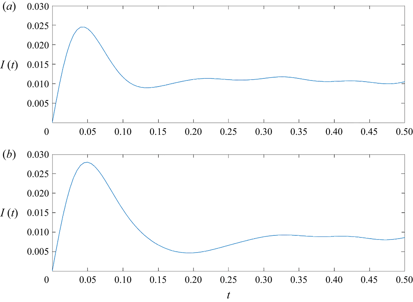
After an equilibration period of 3000 LJ time units to ensure isothermal conditions, the resistance was calculated by numerical integration of the heat-flux autocorrelation trace. Figure 1 shows the result of two such calculations at different conditions. The MD estimate for  $R_K$ was calculated by inserting the result for
 $\int _0^\infty \langle q(t)q(0)\rangle \,{\rm d}t$ into (2.1).
Simulation results for  $I(t)=\int _0^t \psi (t')\,{\rm d}t'$ as a function of non-dimensional time (see § 3) for different conditions: (a)
 $n=0.64$,
 $T=1.2$,
 $C_{wf}=1$ and
 $\varepsilon _{wf}=0.4$; and (b)
 $n=0.8$,
 $T=1.0$,
 $C_{wf}=0.6$ and
 $\varepsilon _{wf}=1$.

Simulations were performed for a wide variety of conditions. Our results are presented in the next subsection and compared with the model (2.15) with  $D=12$; this value was chosen as the one which gives good overall agreement with the MD data. Values for
 $M_\infty$ and
 $\langle \sum _i|{\boldsymbol F_w}|^2_i\rangle$ for use in (2.15) were calculated from MD simulations, while the thermal conductivity of the fluid was calculated using the correlation of Bugel & Galliero (Reference Bugel and Galliero2008).
3.2. Discussion of results
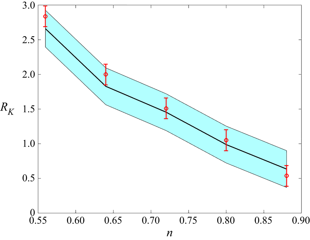
Figure 2 shows the Kapitza resistance as a function of the fluid density,  $n$, at
 $T=1.5$ with
 $\varepsilon _{wf}=1$ and
 $C_{wf}=0.6$. Here,
 $n$ denotes the nominal number density, defined as the ratio of the number of fluid atoms to the fluid volume,
 $V=A L$, where
 $L$ is the distance between the two walls. Although the density is not homogeneous in the vicinity of the wall (Wang & Hadjiconstantinou Reference Wang and Hadjiconstantinou2017), our results below suggest that use of the nominal density leads to a sufficiently accurate description. The monotonically decreasing resistance as a function of fluid density observed in figure 2 is in agreement with the very careful work of Alosious et al. (Reference Alosious, Kannam, Sathian and Todd2019). This behaviour can be understood by noting that the dependence of the relaxation time scale
 $\kappa /M_\infty$ on the fluid density is much weaker than that of the TSWF, which is a monotonically increasing function of the fluid density. We also observe that the model (2.15) matches the simulation results closely.
Kapitza resistance as a function of fluid density at  $T=1.5$,
 $\varepsilon _{wf}=1$ and
 $C_{wf}=0.6$. MD simulation results are shown in red symbols, while the predictions and uncertainty associated with model (2.15) are shown by the black line and blue shading, respectively.

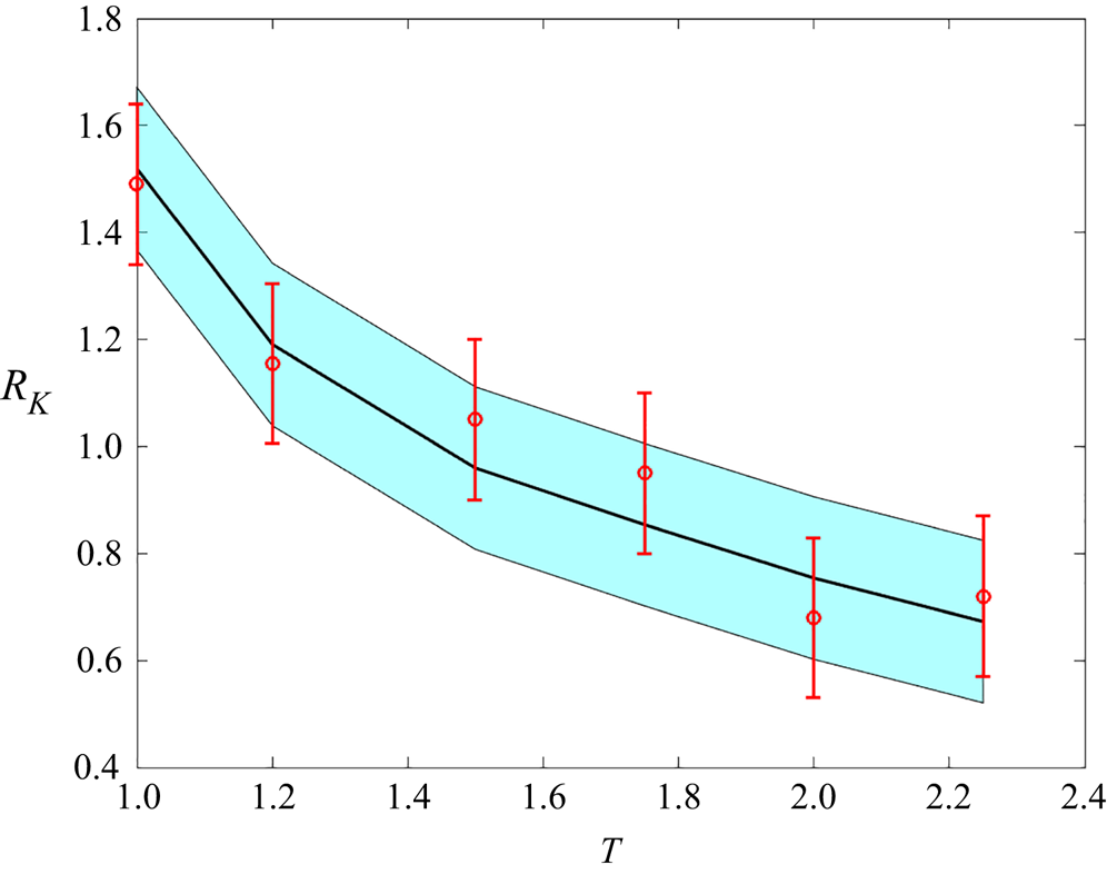
The temperature dependence of the Kapitza resistance observed in figure 3 is in line with previous work (Song & Min Reference Song and Min2013; Alosious et al. Reference Alosious, Kannam, Sathian and Todd2019) and in good agreement with model (2.15), which can also provide more insight into the origins of this behaviour. According to (2.15), the temperature dependence of the Kapitza resistance is a result of competition between three factors, namely, the explicit dependence of  $R_K$ on
 $T$, the temperature dependence of the relaxation time scale
 $\kappa /M_\infty$ and the temperature dependence of the TSWF, the latter being a strongly increasing function of temperature. The monotonic decrease of the resistance as a function of temperature observed here and characterized in detail by Song & Min (Reference Song and Min2013) can thus be understood by noting that, at these conditions, the relaxation time scale
 $\kappa /M_\infty$ is very weakly decreasing as a function of temperature.
Kapitza resistance as a function of temperature with  $n=0.8$,
 $\varepsilon _{wf}=1$ and
 $C_{wf}=0.6$. MD simulation results are shown in red symbols, while the predictions and uncertainty associated with model (2.15) are shown by the black line and blue shading, respectively.

The dependence of the Kapitza resistance on  $\varepsilon _{wf}$ and
 $C_{wf}$ is simple to understand qualitatively, since both these parameters only affect the TSWF. Specifically, the TSWF is a monotonically increasing function of both
 $\varepsilon _{wf}$ and
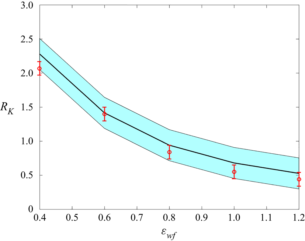
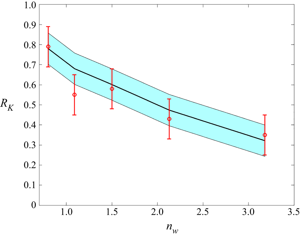
 $C_{wf}$, making the Kapitza resistance a monotonically decreasing function of these parameters, as would be expected from previous work. Figures 4 and 5 show this dependence for
 $T=1.2$ and
 $n=0.64$. The agreement between the model and the simulation results is very good in both cases.
Kapitza resistance as a function of the fluid–solid interaction strength at  $T=1.2$,
 $n=0.64$ with
 $C_{wf}=1$. MD simulation results are shown in red symbols, while the predictions and uncertainty associated with model (2.15) are shown by the black line and blue shading, respectively.

Kapitza resistance as a function of the wall density at  $T=1.2$,
 $n=0.64$ with
 $\varepsilon _{wf}=1$. MD simulation results are shown in red symbols, while the predictions and uncertainty associated with model (2.15) are shown by the black line and blue shading, respectively.

4. Discussion
We have developed and validated a quantitative model for the Kapitza resistance at a fluid–solid interface. The agreement between the model and simulation results is very encouraging and suggests that predictive calculations of the Kapitza resistance based on first-principles information on the fluid–solid system are possible, at least for simple fluids. Extension of this approach to more complex fluid–solid systems (see Guo et al. (Reference Guo, Surblys, Matsubara, Kawagoe and Ohara2020) for example) is a clear next step.
In addition to an accurate quantitative description, the model offers physical insight into the primary factors that affect the behaviour of the Kapitza resistance. The model shows that, beyond the primary system properties ( $m$ and
 $T$), the resistance is determined by two composite properties, namely, the TSWF and the thermal relaxation time
 $I$. The TSWF, the primary factor affecting variations in the value of the resistance, is essentially a measure of the strength of interaction between the wall and fluid; a reduced interaction increases the thermal resistance and vice versa. This insight can be used to explain the recent observations (Alosious et al. Reference Alosious, Kannam, Sathian and Todd2021) on the dependence of
 $R_K$ on nanotube curvature and number of wall layers. The thermal relaxation time, or at least its approximation by
 $\kappa /D M_\infty$, is a property of the fluid only. Increasing the relaxation time reduces the thermal resistance and vice versa, although it should be noted that, as observed before, the ratio
 $\kappa / M_\infty$ appears to be relatively insensitive to variations in the fluid state.
Although both the TSWF and  $I$ can be calculated from MD simulations, as was the case in § 3, it would be preferable if theoretical expressions could be developed for their direct calculation. The approach of § 2.3 is one possible route; it can be completed by characterization of the liquid density profile in the wall vicinity and including the effect of wall structure. Our MD results show that expression (2.20) predicts the dependence of the TSWF on system parameters correctly, at least qualitatively. For the thermal modulus, we note that expressions for its mechanical analogues, the high-frequency shear and bulk moduli,
 $G_\infty$ and
 $K_\infty$, respectively, as a function of the fluid state, were developed a long time ago by Zwanzig & Mountain (Reference Zwanzig and Mountain1965). Unfortunately, the only expression for the thermal modulus that the authors are aware of (Egelstaff Reference Egelstaff1994) is very approximate. We finally note that, since the thermal modulus is essentially a measure of the equilibrium fluctuations of the volume-averaged heat-flux vector, it could also be useful for developing statistical error estimates for the heat-flux vector in MD simulations using the procedure developed by Hadjiconstantinou et al. (Reference Hadjiconstantinou, Garcia, Bazant and He2003).
Perhaps the most remarkable finding in this work is the relative success of the approximation  $I=\kappa /D M_\infty$, which enables the closed-form expression (2.15). Although physically motivated, further work is needed to understand the extent of its generality and develop robust approaches for calculating the value of coefficient
 $D$ from first principles.
Acknowledgments
The authors would like to thank Dr G. Wang for many useful discussions.
Funding
This material is based upon work supported by the Department of Energy, National Nuclear Security Administration under Award Number DE-NA0003965.
Declaration of interests
The authors report no conflict of interest.