1 Introduction
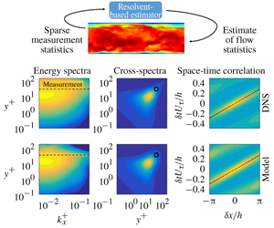
Practical limitations in both experiments and simulations can lead to partial knowledge of flow statistics. For example, an array of probes in an experiment provides information at a limited number of spatial locations and for a single flow quantity, e.g. velocity from hot-wires or pressure from microphones. Similarly, particle image velocimetry might provide velocity data, but not thermodynamic quantities, in a limited field of view. In simulations, one may wish to know flow statistics in a region that is not adequately resolved by the computational grid, such as unresolved near-wall regions. A Reynolds averaged Navier–Stokes simulation might provide mean flow data but not temporal statistics.
The ability to use available data to estimate the statistics of flow quantities that are not directly accessible would be useful in each of these situations. For example, such a method could enable recovery of full-field statistics from a discrete set of measurements, estimates of the statistics of one variable from measurement of another or estimates for a region outside of the field of measurement or computational domain.
Several methods for estimating unknown flow statistics from a limited set of known entries have recently been developed. Beneddine et al. (Reference Beneddine, Sipp, Arnault, Dandois and Lesshafft2016) proposed a method for estimating unknown power spectral densities (PSDs) using knowledge of the mean flow field and power spectra at a few locations. This is accomplished using a least-squares fit at each frequency between the known power spectra and the leading singular response mode obtained from the resolvent operator (McKeon & Sharma Reference McKeon and Sharma2010), which is derived from the linearized Navier–Stokes equations. This strategy explicitly assumes that the spectral content at frequencies of interest is dominated by the leading resolvent mode, and the method performs well when the matching points are located in regions where this hypothesis is valid. Specifically, excellent PSD estimates were obtained for the flow over a backward-facing step (Beneddine et al. Reference Beneddine, Sipp, Arnault, Dandois and Lesshafft2016) and an initially laminar jet (Beneddine et al. Reference Beneddine, Yegavian, Sipp and Leclaire2017). A similar approach was contemporaneously proposed by Gómez et al. (Reference Gómez, Blackburn, Rudman, Sharma and McKeon2016a), but their formulation performed the least-squares fit in the time domain, with a focus on obtaining a low-rank representation of time histories rather than statistics. This approach was used by the authors to estimate oscillation in a cavity flow (Gómez et al. Reference Gómez, Blackburn, Rudman, Sharma and McKeon2016a) and aerodynamic forces on a bluff body (Gómez, Sharma & Blackburn Reference Gómez, Sharma and Blackburn2016b).
Zare, Jovanović & Georgiou (Reference Zare, Jovanović and Georgiou2017) developed a method that uses arbitrary known entries in the spatial covariance tensor to estimate the remaining unknown entries. Their approach is also based on linearized flow equations and entails solving a convex optimization problem that determines a matrix controlling the structure and statistics of the associated nonlinear forcing terms. The optimization problem is subject to two constraints on the estimated covariance tensor: it must reproduce the known entries and obey a Lyapunov equation that relates the forcing and flow statistics. Solving the constrained optimization problem requires a customized algorithm (Zare et al. Reference Zare, Chen, Jovanović and Georgiou2017; Zare et al. Reference Zare, Jovanović and Georgiou2017). The method provides estimates of the unknown entries of the covariance tensor as well as a stochastic dynamical model for the forcing that can be used for model-based estimation and control.
The objective of the present paper is to build on these previous methods to estimate unknown two-point space–time flow statistics. Both the PSDs (one-point temporal statistics) and spatial covariances (two-point spatial statistics) are subsets of two-point space–time correlations, so our approach represents a generalization of these previous methods in the sense that it directly targets the more general two-point space–time flow statistics. This is an important step since two-point space–time statistics contain additional, fundamental information about the flow. In particular, they carry information about coherent motions within the flow, and can even be used to define the concept of a coherent structure (Towne, Schmidt & Colonius Reference Towne, Schmidt and Colonius2018). Moreover, space–time correlations can be used to obtain time-domain estimates of the flow state via convolution with a time-varying input signal (Sasaki et al. Reference Sasaki, Piantanida, Cavalieri and Jordan2017), which enables the development of real-time modelling and flow-control strategies.
The method developed in this paper borrows ideas from each of the previously mentioned methods. Like Beneddine et al. (Reference Beneddine, Sipp, Arnault, Dandois and Lesshafft2016) and Gómez et al. (Reference Gómez, Blackburn, Rudman, Sharma and McKeon2016a), our method is built upon the resolvent formalism of McKeon & Sharma (Reference McKeon and Sharma2010). The resolvent operator is derived from the Navier–Stokes equations linearized about the turbulent mean flow and constitutes a transfer function in the frequency domain between terms that are nonlinear and linear with respect to fluctuations to the mean. Resolvent analysis has proven to be a useful tool for understanding and modelling a wide range of flows, including wall-bounded flows (Sharma & McKeon Reference Sharma and McKeon2013; Morra et al. Reference Morra, Semeraro, Henningson and Cossu2019), free-shear flows (Jeun, Nichols & Jovanović Reference Jeun, Nichols and Jovanović2016; Schmidt et al. Reference Schmidt, Towne, Rigas, Colonius and Brès2018) and aerodynamic wakes (Thomareis & Papadakis Reference Thomareis and Papadakis2018; Symon, Sipp & McKeon Reference Symon, Sipp and McKeon2019; Yeh & Taira Reference Yeh and Taira2019). Whereas Beneddine et al. (Reference Beneddine, Sipp, Arnault, Dandois and Lesshafft2016) constructed their model using only the first singular mode of the resolvent operator (obtained via singular value decomposition), our model relaxes this a priori assumption and allows the known data to self-select the relevant portion of the resolvent operator. This makes the method more applicable to turbulent flows, in which the leading resolvent mode may account for only a modest fraction of the total flow energy (Schmidt et al. Reference Schmidt, Towne, Rigas, Colonius and Brès2018), and allows us to extend the method to cross-spectra in addition to power spectra. Due to its connection with the resolvent operator, we refer to our method as resolvent-based estimation.
Our approach also follows the underlying strategy employed by Zare et al. (Reference Zare, Jovanović and Georgiou2017) of using the known data to infer the statistics of the unknown nonlinear terms that act as a forcing on the linearized equations. Both methods can be used to estimate space–time flow statistics, but the two approaches use different types of input data, which leads to substantial algorithmic differences. The method of Zare et al. (Reference Zare, Jovanović and Georgiou2017) uses arbitrary entries of the spatial covariance tensor, which are spatial (time-integrated) quantities and need not correspond to a fixed set of measurement probes. For example, the authors developed a model for a channel flow using the one-point velocity variance and covariance terms at all wall-normal positions within the channel, but without using two-point correlations. The trade-off of these benefits is the algorithmic complexity mentioned earlier. In contrast, our method requires two-point space–time statistics as input. This could be challenging in some applications, but in many cases the same data used to compute the simpler spatial statistics can be used to obtain the two-point space–time statistics as well. This is the case whenever measurements at multiple locations are obtained simultaneously, e.g. by an array of probes or by sampling numerical data, and two-point space–time statistics can always be obtained using just two concurrent measurements. A benefit of using space–time data as input is that the resulting formulation is algorithmically simple, requiring only basic linear algebra manipulations.
The objective of our method is fundamentally different from previous studies that have used resolvent analysis to obtain low-rank reconstructions of known data. For example, Moarref et al. (Reference Moarref, Jovanović, Tropp, Sharma and McKeon2014) solved a convex optimization problem to determine expansion coefficients for a small set of leading resolvent modes that optimally reproduced known power spectra for a turbulent channel flow. Alternatively, Jeun et al. (Reference Jeun, Nichols and Jovanović2016) used data from a large-eddy simulation of a turbulent jet to directly compute the expansion coefficients and obtained a low-rank reconstruction of the power spectra in the acoustic field by retaining a limited number of terms in the expansion. Similarly, Morra et al. (Reference Morra, Semeraro, Henningson and Cossu2019) obtained a low-rank reconstruction of cross-spectral densities in a turbulent channel flow by computing the necessary expansion coefficients from direct numerical simulation data. Rather than reconstructing known statistics, our objective is to use limited known data to estimate unknown flow statistics.
The objective and capabilities of our method are also fundamentally different from those of the classical method of linear stochastic estimation (Adrian Reference Adrian1994; Bonnet et al. Reference Bonnet, Cole, Delville, Glauser and Ukeiley1994) and related approaches that have recently been investigated (e.g. Encinar, Lozano-Durén & Jiménez Reference Encinar, Lozano-Durén and Jiménez2018). In these methods, cross-correlations between input quantities (the measurements) and output quantities of interest (unknown flow quantities) must be known a priori and are used to estimate instantaneous values or conditional averages for the quantities of interest. In contrast, our method assumes no knowledge of the output statistics (or its cross-correlation with input quantities), and instead uses input data (along with mean flow data) to estimate space–time statistics of the output quantities of interest. Accordingly, our method could in fact be used to obtain an estimate of the statistics required to perform linear stochastic estimation.
The remainder of this paper is organized as follows. The method is derived and described in § 2 and demonstrated in § 3 using two examples: a simple model problem given by the Ginzburg–Landau equation and a turbulent channel flow. Finally, § 4 summarizes the paper and discusses further improvements and applications of the method.
2 Method
Our method for estimating space–time flow statistics from limited measurements is developed in this section. After precisely defining the objective, we develop our approach to the problem and provide some alternative interpretations of the method, which help to elucidate its properties.
2.1 Objective
Consider a state vector of flow variables  $\boldsymbol{q}(\boldsymbol{x},t)$ that describe a flow, e.g. velocities and thermodynamic variables. The independent variables
 $\boldsymbol{x}$ and
 $t$ represent the spatial dimensions of the problem and time, respectively. Now suppose that the two-point space–time statistics are known for a reduced set of variables
 $$\begin{eqnarray}\boldsymbol{y}={\mathcal{C}}\boldsymbol{q},\end{eqnarray}$$
where the linear operator  ${\mathcal{C}}(\boldsymbol{x})$ selects any desired subset or linear combination of
 $\boldsymbol{q}$. The problem objective can now be precisely stated in terms of two-point space–time correlation tensors,
 $$\begin{eqnarray}\displaystyle ~\displaystyle \text{given}\quad \unicode[STIX]{x1D63E}_{\boldsymbol{y}\boldsymbol{y}}(\boldsymbol{x},\boldsymbol{x}^{\prime },\unicode[STIX]{x1D70F}) & = & \displaystyle E\{\boldsymbol{y}(\boldsymbol{x},t)\boldsymbol{y}^{\ast }(\boldsymbol{x}^{\prime },t+\unicode[STIX]{x1D70F})\},\end{eqnarray}$$
 $$\begin{eqnarray}\displaystyle \displaystyle \text{estimate}\quad \unicode[STIX]{x1D63E}_{\boldsymbol{q}\boldsymbol{q}}(\boldsymbol{x},\boldsymbol{x}^{\prime },\unicode[STIX]{x1D70F}) & = & \displaystyle E\{\boldsymbol{q}(\boldsymbol{x},t)\boldsymbol{q}^{\ast }(\boldsymbol{x}^{\prime },t+\unicode[STIX]{x1D70F})\}.\end{eqnarray}$$
 $E\{\cdot \}$ is the expectation operator over time and the asterisk superscript indicates a Hermitian transpose. By defining the correlation tensors in this manner, we have restricted our attention to statistically stationary flows.
Using the relationship between space–time correlation tensors and the cross-spectral density (CSD) tensors
 $$\begin{eqnarray}\unicode[STIX]{x1D64E}(\boldsymbol{x},\boldsymbol{x}^{\prime },\unicode[STIX]{x1D714})=\int _{-\infty }^{\infty }\unicode[STIX]{x1D63E}(\boldsymbol{x},\boldsymbol{x}^{\prime },\unicode[STIX]{x1D70F})\text{e}^{-\text{i}\unicode[STIX]{x1D714}\unicode[STIX]{x1D70F}}\,\text{d}\unicode[STIX]{x1D70F},\end{eqnarray}$$
this objective can be equivalently stated in the frequency domain for statistically stationary flows,
 $$\begin{eqnarray}\displaystyle \displaystyle \text{given}\qquad \unicode[STIX]{x1D64E}_{\boldsymbol{y}\boldsymbol{y}}(\boldsymbol{x},\boldsymbol{x}^{\prime },\unicode[STIX]{x1D714}) & = & \displaystyle E\{\hat{\boldsymbol{y}}(\boldsymbol{x},\unicode[STIX]{x1D714})\hat{\boldsymbol{y}}^{\ast }(\boldsymbol{x}^{\prime },\unicode[STIX]{x1D714})\},\end{eqnarray}$$
 $$\begin{eqnarray}\displaystyle \displaystyle \text{estimate}\qquad \unicode[STIX]{x1D64E}_{\boldsymbol{q}\boldsymbol{q}}(\boldsymbol{x},\boldsymbol{x}^{\prime },\unicode[STIX]{x1D714}) & = & \displaystyle E\{\hat{\boldsymbol{q}}(\boldsymbol{x},\unicode[STIX]{x1D714})\hat{\boldsymbol{q}}^{\ast }(\boldsymbol{x}^{\prime },\unicode[STIX]{x1D714})\},\end{eqnarray}$$
 $\hat{\boldsymbol{y}}(\boldsymbol{x},\unicode[STIX]{x1D714})$ and
 $\hat{\boldsymbol{q}}(\boldsymbol{x},\unicode[STIX]{x1D714})$ are the temporal Fourier transforms of
 $\boldsymbol{y}$ and
 $\boldsymbol{q}$, respectively, and the expectation is now taken over realizations of the flow (Bendat & Piersol Reference Bendat and Piersol1990).
2.2 Approach
Our approach to this problem relies on the resolvent operator obtained from the linearized flow equations and its connection with the remaining nonlinear terms (McKeon & Sharma Reference McKeon and Sharma2010). Accordingly, we call our method resolvent-based estimation. Begin with nonlinear flow equations of the form
 $$\begin{eqnarray}{\mathcal{G}}\frac{\unicode[STIX]{x2202}\boldsymbol{q}}{\unicode[STIX]{x2202}t}=\boldsymbol{{\mathcal{F}}}(\boldsymbol{q}),\end{eqnarray}$$
where  ${\mathcal{G}}$ and
 $\boldsymbol{{\mathcal{F}}}$ are linear and nonlinear operators, respectively. Both compressible and incompressible Navier–Stokes equations can be cast in this form, and
 ${\mathcal{G}}$ is singular in the incompressible case to account for the algebraic divergence-free condition. Alternatively, the incompressible equations can be written with a non-singular
 ${\mathcal{G}}$ by projecting into a divergence-free basis to eliminate the continuity equation (Meseguer & Trefethen Reference Meseguer and Trefethen2003). Additional transport equations can also be included.
Applying the Reynolds decomposition
 $$\begin{eqnarray}\boldsymbol{q}(\boldsymbol{x},t)=\bar{\boldsymbol{q}}(\boldsymbol{x})+\boldsymbol{q}^{\prime }(\boldsymbol{x},t),\end{eqnarray}$$
where  $\bar{\boldsymbol{q}}(\boldsymbol{x})$ is the mean (time-averaged) flow, to (2.5) and isolating the terms that are linear in
 $\boldsymbol{q}^{\prime }$ yields an equation of the form
 $$\begin{eqnarray}{\mathcal{G}}\frac{\unicode[STIX]{x2202}\boldsymbol{q}^{\prime }}{\unicode[STIX]{x2202}t}-{\mathcal{A}}(\bar{\boldsymbol{q}})\boldsymbol{q}^{\prime }=\boldsymbol{f}(\bar{\boldsymbol{q}},\boldsymbol{q}^{\prime }),\end{eqnarray}$$
where
 $$\begin{eqnarray}{\mathcal{A}}(\bar{\boldsymbol{q}})=\frac{\unicode[STIX]{x2202}\boldsymbol{{\mathcal{F}}}}{\unicode[STIX]{x2202}\boldsymbol{q}}(\bar{\boldsymbol{q}})\end{eqnarray}$$
is the linearized Navier–Stokes operator and  $\boldsymbol{f}$ contains the remaining nonlinear terms. Similarly, equation (2.1) becomes
 $$\begin{eqnarray}\boldsymbol{y}^{\prime }={\mathcal{C}}\boldsymbol{q}^{\prime }.\end{eqnarray}$$
In the frequency domain, equations (2.7) and (2.9) can be manipulated to give
 $$\begin{eqnarray}\displaystyle & \displaystyle \hat{\boldsymbol{y}}={\mathcal{R}}_{y}\,\hat{\boldsymbol{f}}, & \displaystyle\end{eqnarray}$$
 $$\begin{eqnarray}\displaystyle & \displaystyle \hat{\boldsymbol{q}}={\mathcal{R}}_{q}\,\hat{\boldsymbol{f}}, & \displaystyle\end{eqnarray}$$
 $$\begin{eqnarray}\displaystyle & \displaystyle {\mathcal{R}}_{\boldsymbol{y}}(\boldsymbol{x},\unicode[STIX]{x1D714})=\,{\mathcal{C}}(\text{i}\unicode[STIX]{x1D714}{\mathcal{G}}-{\mathcal{A}})^{-1}, & \displaystyle\end{eqnarray}$$
 $$\begin{eqnarray}\displaystyle & \displaystyle {\mathcal{R}}_{\boldsymbol{q}}(\boldsymbol{x},\unicode[STIX]{x1D714})=\,(\text{i}\unicode[STIX]{x1D714}{\mathcal{G}}-{\mathcal{A}})^{-1} & \displaystyle\end{eqnarray}$$
 $\hat{\boldsymbol{y}}$ and
 $\hat{\boldsymbol{q}}$, respectively. Strictly speaking, only
 ${\mathcal{R}}_{\boldsymbol{q}}$ is a formal resolvent operator, but for simplicity we will use this terminology for both operators in (2.11). We note that
 ${\mathcal{R}}_{\boldsymbol{y}}$ bears resemblance to the component-wise input–output operators studied by Jovanović & Bamieh (Reference Jovanović and Bamieh2005) and Schmid (Reference Schmid2007), except that here we use
 ${\mathcal{C}}$ to select a sparse set of measurements rather than individual, but globally defined, components of the velocity vector.
Using (2.4) and (2.10), the CSD tensors can be written in terms of these resolvent operators as
 $$\begin{eqnarray}\displaystyle & \displaystyle \unicode[STIX]{x1D64E}_{\boldsymbol{y}\boldsymbol{y}}=\,{\mathcal{R}}_{\boldsymbol{y}}\unicode[STIX]{x1D64E}_{\boldsymbol{f}\boldsymbol{f}}{\mathcal{R}}_{\boldsymbol{y}}^{\ast }, & \displaystyle\end{eqnarray}$$
 $$\begin{eqnarray}\displaystyle & \displaystyle \unicode[STIX]{x1D64E}_{\boldsymbol{q}\boldsymbol{q}}=\,{\mathcal{R}}_{\boldsymbol{q}}\unicode[STIX]{x1D64E}_{\boldsymbol{f}\boldsymbol{f}}{\mathcal{R}}_{\boldsymbol{q}}^{\ast }, & \displaystyle\end{eqnarray}$$
 $\unicode[STIX]{x1D64E}_{\boldsymbol{f}\boldsymbol{f}}(\boldsymbol{x},\boldsymbol{x}^{\prime },\unicode[STIX]{x1D714})=E\{\,\hat{\boldsymbol{f}}(\boldsymbol{x},\unicode[STIX]{x1D714})\hat{\boldsymbol{f}}^{\ast }(\boldsymbol{x}^{\prime },\unicode[STIX]{x1D714})\}$ is the CSD tensor of the nonlinear term
 $\boldsymbol{f}$ (Semeraro et al. Reference Semeraro, Jaunet, Jordan, Cavalieri and Lesshafft2016; Towne, Brès & Lele Reference Towne, Brès and Lele2016; Towne et al. Reference Towne, Schmidt and Colonius2018). We emphasize that no approximation has been made to this point; equation (2.12) is an exact expression of the Navier–Stokes equations for statistically stationary flows.
To obtain an approximation of the desired statistics  $\unicode[STIX]{x1D64E}_{\boldsymbol{q}\boldsymbol{q}}$, we use the known statistics
 $\unicode[STIX]{x1D64E}_{\boldsymbol{y}\boldsymbol{y}}$ to estimate
 $\unicode[STIX]{x1D64E}_{\boldsymbol{f}\boldsymbol{f}}$. The salient question then becomes: how much can we learn about
 $\unicode[STIX]{x1D64E}_{\boldsymbol{f}\boldsymbol{f}}$ from
 $\unicode[STIX]{x1D64E}_{\boldsymbol{y}\boldsymbol{y}}$? An answer is provided by examining the singular value decomposition (SVD)
 $$\begin{eqnarray}\displaystyle {\mathcal{R}}_{\boldsymbol{y}} & = & \displaystyle \unicode[STIX]{x1D650}_{\boldsymbol{y}}\unicode[STIX]{x1D72E}_{\boldsymbol{y}}\unicode[STIX]{x1D651}_{\boldsymbol{y}}^{\ast }\end{eqnarray}$$
 $$\begin{eqnarray}\displaystyle & = & \displaystyle \unicode[STIX]{x1D650}_{\boldsymbol{y}}\left[\begin{array}{@{}cc@{}}\unicode[STIX]{x1D72E}_{1} & \mathbf{0}\end{array}\right][\unicode[STIX]{x1D651}_{1}\,\,\unicode[STIX]{x1D651}_{2}]^{\ast }.\end{eqnarray}$$
 $\unicode[STIX]{x1D651}_{\boldsymbol{y}}$ and
 $\unicode[STIX]{x1D650}_{\boldsymbol{y}}$ correspond to input and output modes that form orthonormal bases for
 $\hat{\boldsymbol{f}}$ and
 $\hat{\boldsymbol{y}}$, respectively. The rectangular matrix
 $\unicode[STIX]{x1D72E}_{\boldsymbol{y}}$ contains the singular values, which determine the gain of each of the input modes to the output. Since the rank of
 ${\mathcal{R}}_{\boldsymbol{y}}$, and thus the number of non-zero singular values, can be no greater than the number of entries in
 $\boldsymbol{y}$, i.e. the number of measurements, many of the input modes have no impact on the output. Accordingly, the SVD can be written in the form of (2.13b), where the diagonal
 $\unicode[STIX]{x1D72E}_{1}$ contains the non-zero singular values and the blocks
 $\unicode[STIX]{x1D651}_{1}$ and
 $\unicode[STIX]{x1D651}_{2}$ contain input modes that have non-zero and zero gain, respectively. It is important to note that these resolvent modes are different from those usually studied, which are given by the SVD of
 ${\mathcal{R}}_{\boldsymbol{q}}$ (e.g. McKeon & Sharma Reference McKeon and Sharma2010; Schmidt et al. Reference Schmidt, Towne, Rigas, Colonius and Brès2018).
The distinction between input modes that do or do not impact the output can be used to isolate the part of  $\unicode[STIX]{x1D64E}_{\boldsymbol{f}\boldsymbol{f}}$ that can be educed from knowledge of
 $\unicode[STIX]{x1D64E}_{\boldsymbol{y}\boldsymbol{y}}$. Since
 $\unicode[STIX]{x1D651}_{\boldsymbol{y}}$ provides a complete basis for
 $\hat{\boldsymbol{f}}$,
 $\unicode[STIX]{x1D64E}_{\boldsymbol{f}\boldsymbol{f}}$ can be expanded as
 $$\begin{eqnarray}\unicode[STIX]{x1D64E}_{\unicode[STIX]{x1D65B}\boldsymbol{f}}=\left[\unicode[STIX]{x1D651}_{1}\,\,\unicode[STIX]{x1D651}_{2}\right]\left[\begin{array}{@{}cc@{}}\unicode[STIX]{x1D641}_{11} & \unicode[STIX]{x1D641}_{12}\\ \unicode[STIX]{x1D641}_{21} & \unicode[STIX]{x1D641}_{22}\end{array}\right][\unicode[STIX]{x1D651}_{1}\,\,\unicode[STIX]{x1D651}_{2}]^{\ast },\end{eqnarray}$$
where the matrices  $\unicode[STIX]{x1D641}_{ij}$ represent correlations between expansion coefficients associated with each input mode (see Towne et al. Reference Towne, Schmidt and Colonius2018). Inserting this expansion into (2.12a) and using (2.13b) to simplify the expression gives rise to the equation
 $$\begin{eqnarray}\unicode[STIX]{x1D64E}_{\boldsymbol{y}\boldsymbol{y}}=\unicode[STIX]{x1D650}_{\boldsymbol{y}}\unicode[STIX]{x1D72E}_{1}\unicode[STIX]{x1D641}_{11}\unicode[STIX]{x1D72E}_{1}\unicode[STIX]{x1D650}_{\boldsymbol{y}}^{\ast }.\end{eqnarray}$$
This means that only the part of  $\unicode[STIX]{x1D64E}_{\boldsymbol{f}\boldsymbol{f}}$ associated with
 $\unicode[STIX]{x1D641}_{11}$ impacts the observed statistics
 $\unicode[STIX]{x1D64E}_{\boldsymbol{y}\boldsymbol{y}}$; the remaining
 $\unicode[STIX]{x1D641}_{ij}$ terms have no impact and are thus unobservable from these known data. Consequently,
 $\unicode[STIX]{x1D641}_{11}$ contains all of the information about
 $\unicode[STIX]{x1D64E}_{\boldsymbol{f}\boldsymbol{f}}$ that can be inferred from
 $\unicode[STIX]{x1D64E}_{\boldsymbol{y}\boldsymbol{y}}$. Using the orthonormality of
 $\unicode[STIX]{x1D650}_{\boldsymbol{y}}$, equation (2.15) gives
 $$\begin{eqnarray}\unicode[STIX]{x1D641}_{11}=\unicode[STIX]{x1D72E}_{1}^{-1}\unicode[STIX]{x1D650}_{\boldsymbol{y}}^{\ast }\unicode[STIX]{x1D64E}_{\boldsymbol{y}\boldsymbol{y}}\unicode[STIX]{x1D650}_{\boldsymbol{y}}\unicode[STIX]{x1D72E}_{1}^{-1}.\end{eqnarray}$$
The remaining terms  $\unicode[STIX]{x1D641}_{22}$ and
 $\unicode[STIX]{x1D641}_{12}=\unicode[STIX]{x1D641}_{21}^{\ast }$ (this equality is required to make
 $\unicode[STIX]{x1D64E}_{\boldsymbol{f}\boldsymbol{f}}$ Hermitian) can be arbitrarily chosen without impacting
 $\unicode[STIX]{x1D64E}_{\boldsymbol{y}\boldsymbol{y}}$, but these terms will impact
 $\unicode[STIX]{x1D64E}_{\boldsymbol{q}\boldsymbol{q}}$ and therefore must be modelled. The simplest choice, and the one used in the remainder of this paper, is to set these unknown terms to zero, leading to the approximation
 $$\begin{eqnarray}\unicode[STIX]{x1D64E}_{\boldsymbol{f}\boldsymbol{f}}\approx \tilde{\unicode[STIX]{x1D64E}}_{\boldsymbol{f}\boldsymbol{f}}=[\unicode[STIX]{x1D651}_{1}\,\,\unicode[STIX]{x1D651}_{2}]\left[\begin{array}{@{}cc@{}}\unicode[STIX]{x1D641}_{11} & \mathbf{0}\\ \boldsymbol{ 0} & \mathbf{0}\end{array}\right][\unicode[STIX]{x1D651}_{1}\,\,\unicode[STIX]{x1D651}_{2}]^{\ast }=\unicode[STIX]{x1D651}_{1}\unicode[STIX]{x1D641}_{11}\unicode[STIX]{x1D651}_{1}^{\ast }.\end{eqnarray}$$
We show in appendix A that this choice is identical to taking the least-squares approximation of  $\unicode[STIX]{x1D64E}_{\boldsymbol{f}\boldsymbol{f}}$, which can be obtained by applying the pseudo-inverse of
 ${\mathcal{R}}_{y}$ and its complex conjugate to the left and right sides of (2.12a), respectively. That is,
 $$\begin{eqnarray}\tilde{\unicode[STIX]{x1D64E}}_{\boldsymbol{f}\boldsymbol{f}}={\mathcal{R}}_{\boldsymbol{y}}^{+}\unicode[STIX]{x1D64E}_{\boldsymbol{y}\boldsymbol{y}}({\mathcal{R}}_{\boldsymbol{y}}^{+})^{\ast },\end{eqnarray}$$
where the plus superscript indicates the pseudo-inverse. Therefore, this approximation corresponds to choosing the smallest forcing (in an appropriate norm) that reproduces the known flow statistics. In what follows, a tilde accent indicates an estimated quantity.
Inserting (2.17) or (2.18) into (2.12b) gives the corresponding approximation of the desired flow statistics
 $$\begin{eqnarray}\unicode[STIX]{x1D64E}_{\boldsymbol{q}\boldsymbol{q}}\approx \tilde{\unicode[STIX]{x1D64E}}_{\boldsymbol{q}\boldsymbol{q}}={\mathcal{R}}_{\boldsymbol{q}}\unicode[STIX]{x1D651}_{1}\unicode[STIX]{x1D641}_{11}\unicode[STIX]{x1D651}_{1}^{\ast }{\mathcal{R}}_{\boldsymbol{q}}^{\ast }={\mathcal{R}}_{\boldsymbol{ q}}{\mathcal{R}}_{\boldsymbol{y}}^{+}\unicode[STIX]{x1D64E}_{\boldsymbol{y}\boldsymbol{y}}({\mathcal{R}}_{\boldsymbol{y}}^{+})^{\ast }{\mathcal{R}}_{\boldsymbol{q}}^{\ast }.\end{eqnarray}$$
By construction, the known statistics used as input are exactly recovered, ensuring that the approximation converges in the limit of full knowledge of the flow statistics. Other approximations can be obtained by choosing the unknown  $\unicode[STIX]{x1D641}_{ij}$ terms differently; a few possibilities are discussed in § 4. The estimated space–time correlation tensor can be recovered from the estimated CSD via the inverse Fourier transform
 $$\begin{eqnarray}\unicode[STIX]{x1D63E}(\boldsymbol{x},\boldsymbol{x}^{\prime },\unicode[STIX]{x1D70F})=\frac{1}{2\unicode[STIX]{x03C0}}\int _{-\infty }^{\infty }\unicode[STIX]{x1D64E}(\boldsymbol{x},\boldsymbol{x}^{\prime },\unicode[STIX]{x1D714})\text{e}^{\text{i}\unicode[STIX]{x1D714}\unicode[STIX]{x1D70F}}\text{d}\unicode[STIX]{x1D714}.\end{eqnarray}$$
The method can also be understood in terms of a resolvent-mode expansion of  $\unicode[STIX]{x1D64E}_{\boldsymbol{q}\boldsymbol{q}}$. The standard resolvent modes associated with the linearized flow equations are defined by the SVD
 ${\mathcal{R}}_{\boldsymbol{q}}=\,\unicode[STIX]{x1D650}_{\boldsymbol{q}}\unicode[STIX]{x1D72E}_{\boldsymbol{q}}\unicode[STIX]{x1D651}_{\boldsymbol{q}}^{\ast }$. Equation (2.19) can then be written as
 $$\begin{eqnarray}\tilde{\unicode[STIX]{x1D64E}}_{\boldsymbol{q}\boldsymbol{q}}=\unicode[STIX]{x1D650}_{\boldsymbol{q}}\unicode[STIX]{x1D72E}_{\boldsymbol{q}}\unicode[STIX]{x1D64E}_{\unicode[STIX]{x1D6FD}\unicode[STIX]{x1D6FD}}\unicode[STIX]{x1D72E}_{\boldsymbol{q}}\unicode[STIX]{x1D650}_{\boldsymbol{q}}^{\ast },\end{eqnarray}$$
where
 $$\begin{eqnarray}\unicode[STIX]{x1D64E}_{\unicode[STIX]{x1D6FD}\unicode[STIX]{x1D6FD}}=\unicode[STIX]{x1D651}_{\boldsymbol{q}}^{\ast }\unicode[STIX]{x1D651}_{1}\unicode[STIX]{x1D641}_{11}\unicode[STIX]{x1D651}_{1}^{\ast }\unicode[STIX]{x1D651}_{\boldsymbol{q}}\end{eqnarray}$$
is the CSD of the expansion coefficients in a resolvent-mode expansion of  $\hat{\boldsymbol{q}}$ (Towne et al. Reference Towne, Schmidt and Colonius2018). In general,
 $\unicode[STIX]{x1D64E}_{\unicode[STIX]{x1D6FD}\unicode[STIX]{x1D6FD}}$ can project onto any of the resolvent output modes in
 $\unicode[STIX]{x1D650}_{\boldsymbol{q}}$. Thus, the known statistics
 $\unicode[STIX]{x1D64E}_{\boldsymbol{y}\boldsymbol{y}}$, through their influence on
 $\unicode[STIX]{x1D641}_{11}$, determine which resolvent modes participate in the estimate of
 $\unicode[STIX]{x1D64E}_{\boldsymbol{q}\boldsymbol{q}}$. This can be contrasted with the rank-1 model described earlier, in which only the leading resolvent mode is allowed to contribute. Similarly, the multi-mode extension of the rank-1 method proposed (but not implemented) by Beneddine et al. (Reference Beneddine, Yegavian, Sipp and Leclaire2017) requires a priori selection of a limited number of modes of
 ${\mathcal{R}}_{\boldsymbol{q}}$. Also note that since our method does not require the SVD of
 ${\mathcal{R}}_{\boldsymbol{q}}$, but only of the low-rank matrix
 ${\mathcal{R}}_{\boldsymbol{y}}$, our method is less computationally expensive than a typical resolvent analysis.
3 Examples
In this section, our method is demonstrated and analysed using two example problems: the complex Ginzburg–Landau equation and a turbulent channel flow.
3.1 Ginzburg–Landau equation
The Ginzburg–Landau equation has been used by several previous authors (e.g. Hunt & Crighton Reference Hunt and Crighton1991; Bagheri et al. Reference Bagheri, Henningson, Hoepffner and Schmid2009; Chen & Rowley Reference Chen and Rowley2011; Towne et al. Reference Towne, Schmidt and Colonius2018) as a convenient one-dimensional model that mimics key properties of the linearized Navier–Stokes operator for real flows, such as a turbulent jet (Schmidt et al. Reference Schmidt, Towne, Rigas, Colonius and Brès2018). The linearized equations can be written in the form of (2.7) with  ${\mathcal{G}}$ equal to the identity matrix and
 $$\begin{eqnarray}{\mathcal{A}}=-\unicode[STIX]{x1D708}\frac{\unicode[STIX]{x2202}}{\unicode[STIX]{x2202}x}+\unicode[STIX]{x1D6FE}\frac{\unicode[STIX]{x2202}^{2}}{\unicode[STIX]{x2202}x^{2}}+\unicode[STIX]{x1D707}(x).\end{eqnarray}$$
Several variants of the function  $\unicode[STIX]{x1D707}(x)$ have been used in the literature; here the quadratic form
 $$\begin{eqnarray}\unicode[STIX]{x1D707}(x)=(\unicode[STIX]{x1D707}_{0}-c_{u}^{2})+\frac{\unicode[STIX]{x1D707}_{2}}{2}x^{2}\end{eqnarray}$$
is adopted (Hunt & Crighton Reference Hunt and Crighton1991; Bagheri et al. Reference Bagheri, Henningson, Hoepffner and Schmid2009; Chen & Rowley Reference Chen and Rowley2011). The parameters in (3.1) and (3.2) are set to similar values as those used by Bagheri et al. (Reference Bagheri, Henningson, Hoepffner and Schmid2009) and Towne et al. (Reference Towne, Schmidt and Colonius2018):  $\unicode[STIX]{x1D708}=2+0.2i$,
 $\unicode[STIX]{x1D6FE}=1-i$,
 $\unicode[STIX]{x1D707}_{0}=0.3$,
 $c_{u}=0.2$,
 $\unicode[STIX]{x1D707}_{2}=-0.01$. Following Bagheri et al. (Reference Bagheri, Henningson, Hoepffner and Schmid2009), the equations are discretized with a pseudo-spectral approach using
 $N=220$ Hermite polynomials.
The discretized equations are stochastically excited in the time domain using forcing terms with prescribed statistics identical to those used by (Towne et al. Reference Towne, Schmidt and Colonius2018). In particular, the forcing is generated by convolving band-limited white noise with a kernel of the form
 $$\begin{eqnarray}g(x,x^{\prime })=\frac{1}{\sqrt{2\unicode[STIX]{x03C0}}\unicode[STIX]{x1D70E}_{f}}\exp \left[-\frac{1}{2}\left(\frac{x-x^{\prime }}{\unicode[STIX]{x1D70E}_{f}}\right)^{2}\right]\exp \left[\text{i}2\unicode[STIX]{x03C0}\frac{x-x^{\prime }}{\unicode[STIX]{x1D706}_{f}}\right],\end{eqnarray}$$
where  $\unicode[STIX]{x1D70E}_{f}$ is the standard deviation of the envelope and
 $\unicode[STIX]{x1D706}_{f}$ is the wavelength of the filter. This leads to a forcing that is white-in-time up to the cutoff frequency but that has non-zero spatial correlation in the form of (3.3) but with
 $\unicode[STIX]{x1D70E}_{f}$ replaced with
 $\sqrt{2}\unicode[STIX]{x1D70E}_{f}$. This form of the forcing statistics is qualitatively similar to those of the nonlinear forcing terms in real flows, such as a turbulent jet (Towne, Brès & Lele Reference Towne, Brès and Lele2017). We use
 $\unicode[STIX]{x1D70E}_{f}=4$ and
 $\unicode[STIX]{x1D706}_{f}=20$.
Although these forcing statistics are prescribed in this model problem and therefore known, this knowledge is not made available to the estimation procedure. The equations are integrated using a fourth-order embedded Runge–Kutta method (Shampine & Reichelt Reference Shampine and Reichelt1997), and a total of  $10\,000$ snapshots of the solution are collected with spacing
 $\unicode[STIX]{x0394}t=0.5$, leading to a Nyquist frequency of
 $\unicode[STIX]{x1D714}_{Nyquist}=2\unicode[STIX]{x03C0}$. The CSD of the solution is computed from these data using Welch’s (Reference Welch1967) method.
For the majority of the following analysis,  $\boldsymbol{y}$ is defined to correspond to data obtained from three probes located at
 $x=-10$, 0 and 10. Other choices are considered in § 3.1.4.
3.1.1 Power spectra
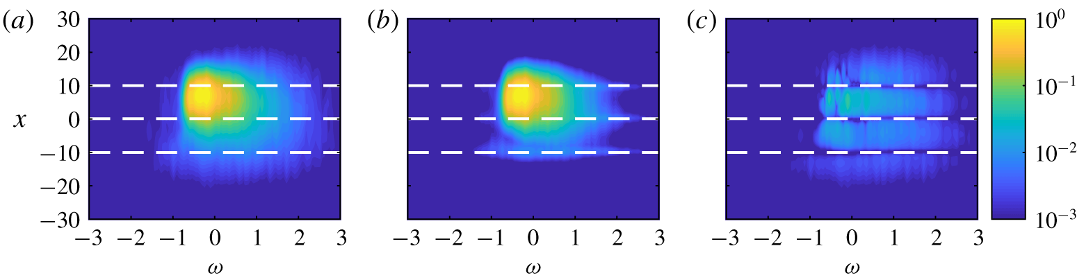
The PSD is contained in the diagonal entries of  $\unicode[STIX]{x1D64E}_{\boldsymbol{q}\boldsymbol{q}}$, i.e.
 $\unicode[STIX]{x1D640}_{\boldsymbol{q}\boldsymbol{q}}(x,\unicode[STIX]{x1D714})=\unicode[STIX]{x1D64E}_{\boldsymbol{q}\boldsymbol{q}}(x,x,\unicode[STIX]{x1D714})$. The true power spectral density for the Ginzburg–Landau model problem is shown as a function of
 $\unicode[STIX]{x1D714}$ and
 $x$ in figure 1(a). A single peak is observed at
 $\unicode[STIX]{x1D714}\approx -0.2$ and
 $x\approx 5$, and the amplitude remains above 1 % of the peak over a range of about
 $-0.75<\unicode[STIX]{x1D714}<1$ and
 $-5<x<15$. The dashed lines show the
 $x$ locations where the data are taken as known, and the estimation procedure will attempt to reconstruct the PSD elsewhere.
Power spectral density (PSD) as a function of  $\unicode[STIX]{x1D714}$ and
 $x$ for the Ginzburg–Landau model problem: (a) true PSD; (b) estimated PSD using three probes at the locations of the dashed lines; (c) difference between the true and estimated PSD.

The approximation of the PSD obtained using these three probes is shown in figure 1(b), and the difference between the true and estimated PSD in shown in figure 1(c). By construction, the approximation is exact at the probe locations. The peak is well captured and the agreement is good in high-energy regions. In the lower-energy regions, the PSD is under-predicted away from the probe locations. This is a consequence of neglecting the undetermined portions of the forcing. It is likely that additional improvements could be obtained by modelling these undetermined portions of the forcing, as discussed in § 4. The total error of the PSD estimate, defined as
 $$\begin{eqnarray}{\displaystyle \frac{\displaystyle \iint |\tilde{\unicode[STIX]{x1D640}}_{\boldsymbol{q}\boldsymbol{q}}(x,\unicode[STIX]{x1D714})-\unicode[STIX]{x1D640}_{\boldsymbol{q}\boldsymbol{q}}(x,\unicode[STIX]{x1D714})|\,\text{d}\unicode[STIX]{x1D714}\,\text{d}x}{\displaystyle \iint \unicode[STIX]{x1D640}_{\boldsymbol{q}\boldsymbol{q}}(x,\unicode[STIX]{x1D714})\,\text{d}\unicode[STIX]{x1D714}\,\text{d}x}},\end{eqnarray}$$
is 4.9 %.
3.1.2 Cross-spectra
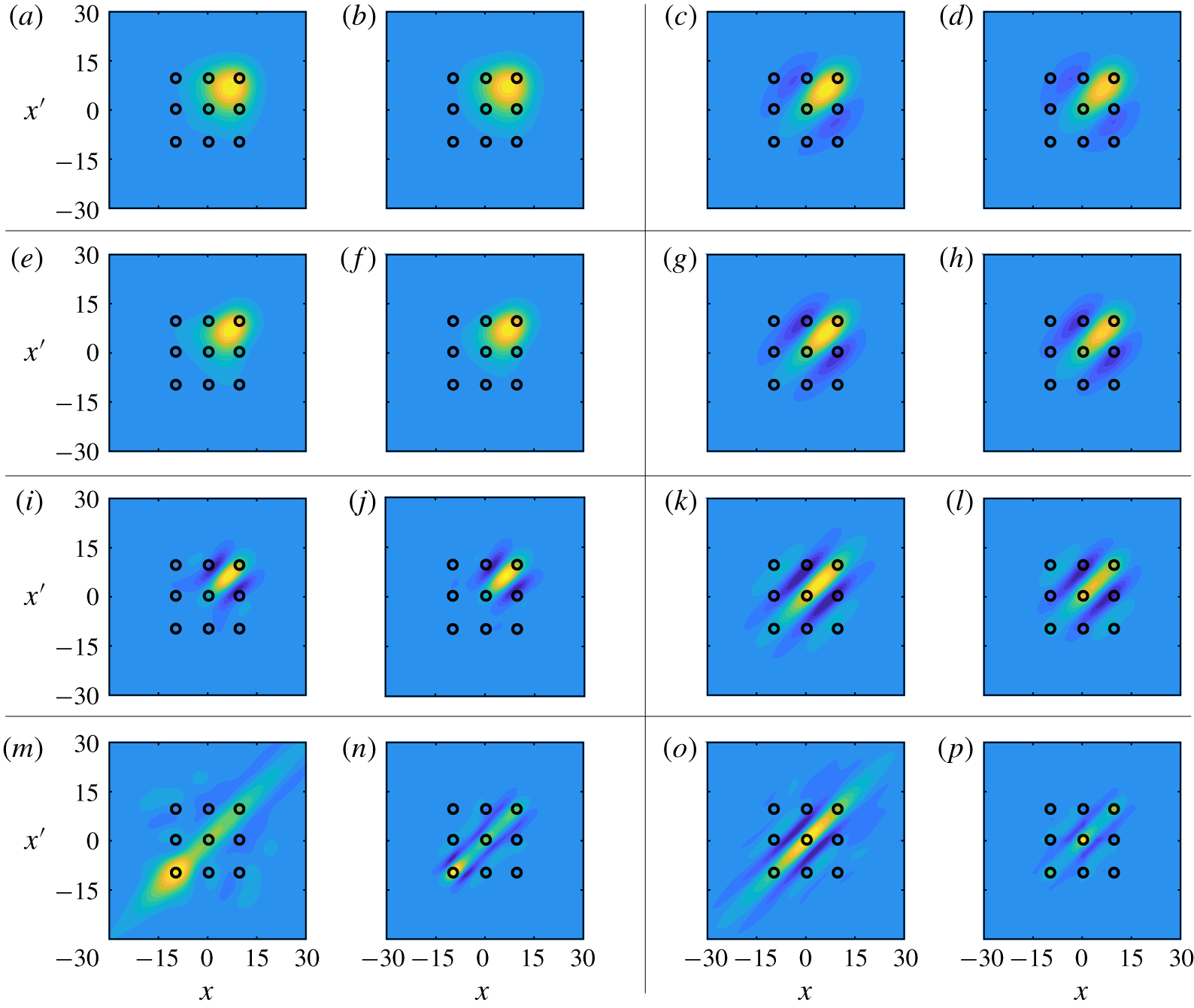
The CSD estimates are evaluated next. Figure 2 compares the real part of the true and modelled CSD at eight frequencies, which are listed in the caption. The contour levels are the same for the true and estimated data at each frequency and range from  $-0.5$ to
 $1$ relative to the maximum value of the true CSD. The circles indicate the locations where the CSD is known and the remaining values are to be estimated. The first six frequencies (panels a–l) fall within the high-energy region observed in figure 1. In these cases, the estimates accurately track the amplitudes, length scales and overall shape of the CSD as a function of frequency. The final two frequencies (panels m–p) fall in low-energy regions. The basic trends in the length scales and shape are still captured, but clear errors can be observed.
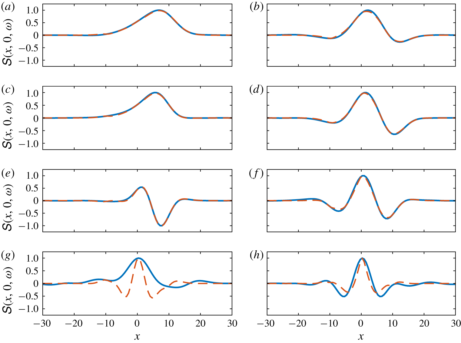
Figure 3 provides a more quantitative assessment of the CSD estimates. Here, the CSD relative to the reference point  $x^{\prime }=0$ is plotted as a function of
 $x$ for the same eight frequencies shown in figure 2. Both the true CSD (solid lines) and estimated CSD (dashed lines) are normalized by the maximum magnitude of the true CSD for each frequency. These plots show that the CSD estimates are quantitatively accurate for the six frequencies in the high-energy region.
Cross-spectral density (CSD) for the frequencies (a,b)  $\unicode[STIX]{x1D714}=0$; (e,f)
 $\unicode[STIX]{x1D714}=-0.2$; (i,j)
 $\unicode[STIX]{x1D714}=-0.6$; (m,n)
 $\unicode[STIX]{x1D714}=-1$; (c,d)
 $\unicode[STIX]{x1D714}=0.4$; (g,h)
 $\unicode[STIX]{x1D714}=0.6$; (k,l)
 $\unicode[STIX]{x1D714}=1$; (o,p)
 $\unicode[STIX]{x1D714}=2$. In each case, the left-hand plot shows the true CSD and the right-hand plot shows the estimated values using three probes, which lead to known CSD values at the locations indicated by the small circles. The contour levels are the same for the true and estimated data at each frequency and range from the minimum to maximum values of the true CSD.

Cross-spectral density (CSD) relative to the reference point  $x^{\prime }=0$ for the frequencies (a)
 $\unicode[STIX]{x1D714}=0$; (c)
 $\unicode[STIX]{x1D714}=-0.2$; (e)
 $\unicode[STIX]{x1D714}=-0.6$; (g)
 $\unicode[STIX]{x1D714}=-1$; (b)
 $\unicode[STIX]{x1D714}=0.4$; (d)
 $\unicode[STIX]{x1D714}=0.6$; (f)
 $\unicode[STIX]{x1D714}=1$; (h)
 $\unicode[STIX]{x1D714}=2$. The solid lines show the true values, and the dashed lines show the estimates values using three probes at
 $x=-10,0$ and 10.

3.1.3 Space–time correlations
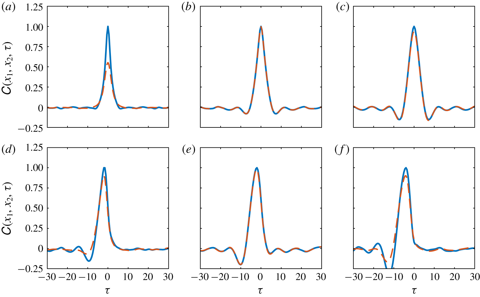
Cross-correlation as a function of time lag  $\unicode[STIX]{x1D70F}$ for (a)
 $x_{1}=x_{2}=-5$; (b)
 $x_{1}=x_{2}=0$; (c)
 $x_{1}=x_{2}=5$; (d)
 $x_{1}=-5$,
 $x_{2}=0$; (e)
 $x_{1}=0$,
 $x_{2}=5$; (d)
 $x_{1}=-5$,
 $x_{2}=5$. The solid lines show the true values, and the dashed lines show the estimates values using three probes at
 $x=-10,0$ and 10. Both the true and estimated curves in each plot have been scaled by the maximum value of the true correlation.

Cross-correlation as a function of  $x$ and
 $x^{\prime }$ for fixed time-lag values (a,b)
 $\unicode[STIX]{x1D70F}=0$; (c,d)
 $\unicode[STIX]{x1D70F}=1$; (e,f)
 $\unicode[STIX]{x1D70F}=2$; (g,h)
 $\unicode[STIX]{x1D70F}=4$; (i,j)
 $\unicode[STIX]{x1D70F}=6$; (k,l)
 $\unicode[STIX]{x1D70F}=10$. In each case, the left-hand plot shows the true correlations, and the right-hand plot shows the estimated values using three probes, which lead to known cross-correlations at the locations indicated by the small circles. The contour levels are the same in each panel and range from zero to the maximum values of the true correlation at
 $\unicode[STIX]{x1D70F}=0$.

The space–time correlation tensor  $\unicode[STIX]{x1D63E}_{\boldsymbol{q}\boldsymbol{q}}$ can be recovered from the cross-spectral density
 $\unicode[STIX]{x1D64E}_{\boldsymbol{q}\boldsymbol{q}}$ using the inverse Fourier transform of (2.3). As an example, figure 4 shows the true (solid lines) and estimated (dashed lines) correlations as a function of time lag
 $\unicode[STIX]{x1D70F}$ for three spatial locations,
 $x=-5$, 0 and 5. These locations correspond to a low-energy region, a probe position and the energy peak, respectively. Each curve has been scaled by the maximum value of the corresponding true correlation.
The one-point autocorrelation for each point is shown in figure 4(a–c). The amplitude of the autocorrelation for the low-energy point at  $x=-5$ (panel a) is significantly under-predicted, but the correlation length scale is well captured. The estimated autocorrelation at
 $x=0$ (panel b) is exact since this point corresponds to one of the probe locations. The autocorrelation at
 $x=5$ (panel c) is accurately estimated apart from a small under-prediction of the peak, which corresponds to an under-prediction of the variance.
The cross-correlations between these three points are shown in figure 4(d–f). The estimates are quite good in all cases, including those involving the low-energy point (panels d and f) and two unknown points (panel f). It is interesting that the cross-correlations involving the low-energy point are more accurate than the autocorrelation at this point. The agreement for the cross-correlation between the known and high-energy points (panel e) is almost perfect.
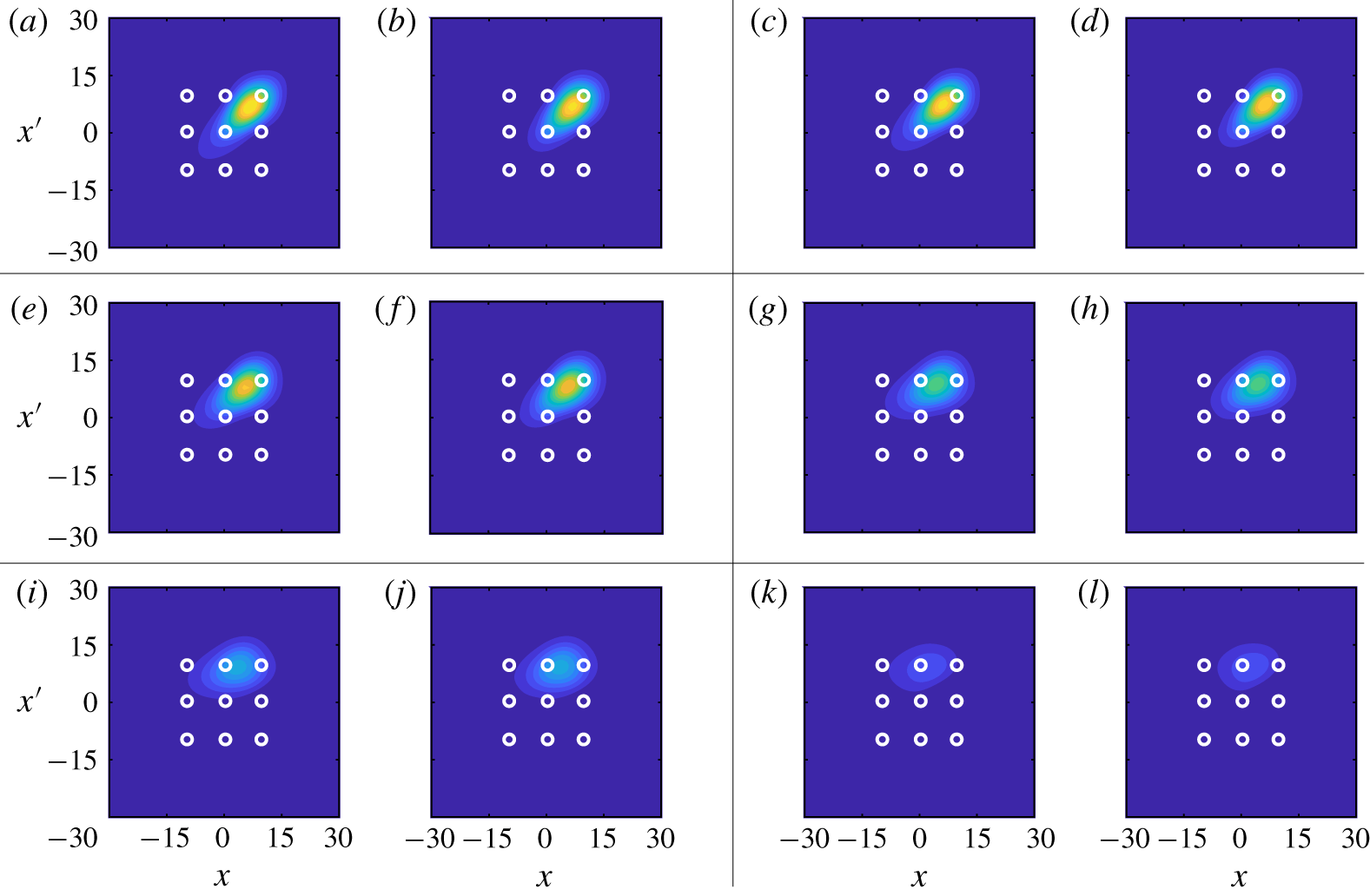
The spatial distribution of the true and estimated cross-correlation tensors at fixed values of the time lag  $\unicode[STIX]{x1D70F}$ is shown in figure 5. The plotted time-lag values range from
 $\unicode[STIX]{x1D70F}=0$ to 10; negative values need not be considered due to the symmetry
 $$\begin{eqnarray}\unicode[STIX]{x1D63E}_{\boldsymbol{q}\boldsymbol{q}}(\boldsymbol{x}_{1},\boldsymbol{x}_{2},-\unicode[STIX]{x1D70F})=\unicode[STIX]{x1D63E}_{\boldsymbol{q}\boldsymbol{q}}^{\ast }(\boldsymbol{x}_{2},\boldsymbol{x}_{1},\unicode[STIX]{x1D70F}).\end{eqnarray}$$
The contour levels are the same in each panel and range from zero to the maximum values of the true correlation at  $\unicode[STIX]{x1D70F}=0$. Again, the circles indicate the locations where the correlations are known, and the remaining values are to be estimated.
The spatial correlation tensor is obtained for  $\unicode[STIX]{x1D70F}=0$ and is shown in figure 5(a). As already observed in figure 4, the amplitudes of the correlations at zero time lag are slightly under predicted, but the spatial shape and overall amplitude are well captured. As the time lag
 $\unicode[STIX]{x1D70F}$ is increased, the estimates faithfully track the changing amplitude and shape of the true correlations up to at least
 $\unicode[STIX]{x1D70F}=10$, by which point the amplitudes of the correlations are small.
3.1.4 Impact of probe location and comparisons with the rank-1 model
Power spectral density as a function of  $\unicode[STIX]{x1D714}$ and
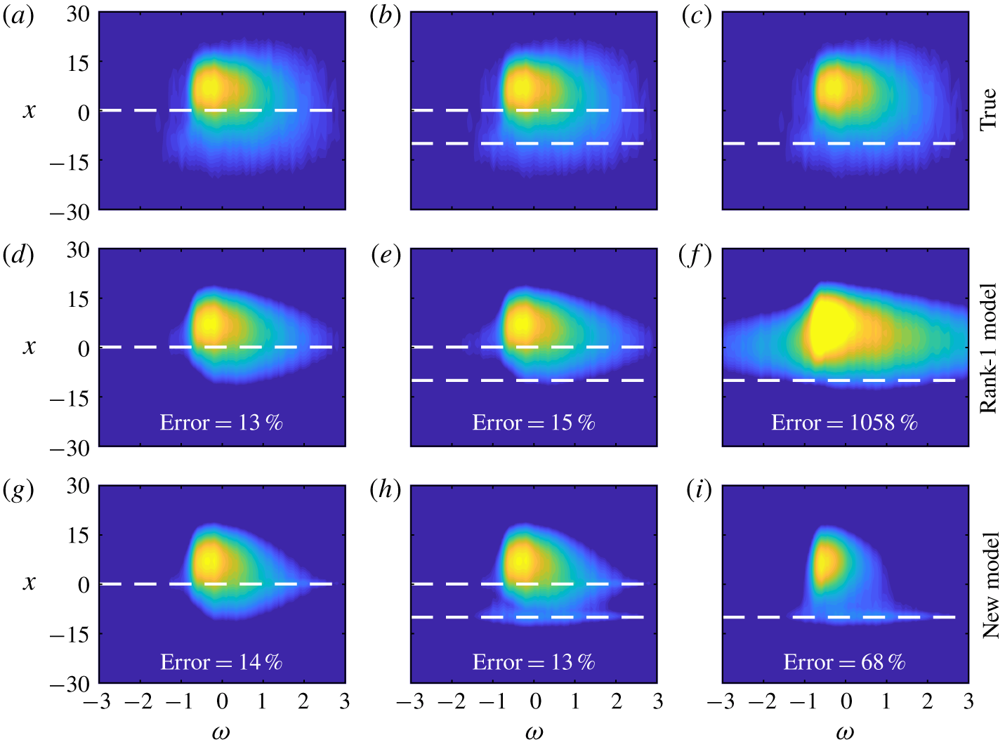
 $x$: (a–c) true values repeated for ease of comparison; (d–f) estimated values from the rank-1 model of Beneddine et al. (Reference Beneddine, Sipp, Arnault, Dandois and Lesshafft2016); (g–i) estimated values from the new model presented in this paper. The estimates are based on the following probe locations: (a,d,g)
 $x=0$; (b,e,h)
 $x=-10$ and 0; (c,f,i)
 $x=-10$. The contour levels are the same as figure 1.

In this section, comparisons are made between the new resolvent-based estimation method described in this paper and the rank-1 method of Beneddine et al. (Reference Beneddine, Sipp, Arnault, Dandois and Lesshafft2016) that was discussed in § 1. Particular attention is given to the impact of the probe location(s) on the accuracy of the estimates provided by these two methods.
We focus on the PSD, which is the target quantity of the rank-1 model. Figure 6 compares the true PSD (a–c) to the estimates from the rank-1 method (d–f) and the new model (g–i) for three different sets of probe locations (columns). The integrated error metric from (3.4) is also reported in the figure for each estimate.
First, a single probe is placed at  $x=0$. In this case, the two methods provide similar estimates. Adding an additional probe in the low-energy region at
 $x=-10$ (second column) increases the error of the rank-1 method. This is an undesirable property; it means that poorly placed probes (where the rank-1 assumption is invalid) can obscure the information provided by well-placed probes (where the assumption is valid). More generally, this is a manifestation of the fact that the rank-1 method does not necessarily converge with increasing input information (Towne et al. Reference Towne, Schmidt and Colonius2018). In contrast, the new method is able to use this additional information to improve the estimate near the second probe without degrading the estimate near the original probe, leading to a small reduction in total error.
In the final case, the original probe at  $x=0$ is removed, leaving a single probe in the low-energy location
 $x=-10$. At this point, the underlying assumption of the rank-1 model – that the solution is dominated by the leading resolvent mode – is false. This is representative of the situation that will be encountered in real turbulent flows. Because of this, the rank-1 method leads to large over-predictions of the PSD and an error in excess of 1000 %. In contrast, the new method is able to use the information provided by this poorly placed probe to provide a reasonable estimate, albeit with higher error than is achieved using a well-placed probe. The moderate under-prediction of the PSD observed in this case can be attributed to neglecting the unobservable portions of
 $\unicode[STIX]{x1D64E}_{\boldsymbol{f}\boldsymbol{f}}$.
3.2 Turbulent channel flow
3.2.1 Flow parameters, simulation and data processing
Next, we apply the our resolvent-based estimation method to an incompressible turbulent channel flow at friction Reynolds number  $Re_{\unicode[STIX]{x1D70F}}=187$, defined in terms of the friction velocity
 $U_{\unicode[STIX]{x1D70F}}$ and the kinematic viscosity
 $\unicode[STIX]{x1D708}$. Wall units, denoted by
 $+$ superscripts, are also defined in terms of
 $U_{\unicode[STIX]{x1D70F}}$ and
 $\unicode[STIX]{x1D708}$. This flow provides a convenient test case for application of the method to a real, nonlinear, turbulent flow. However, it is important to note that the results at this low Reynolds number may or may not extend to higher Reynolds numbers.
The flow is computed via direct numerical simulation (DNS) of the incompressible Navier–Stokes equations in a domain of size  $L_{x}/h=2\unicode[STIX]{x03C0}$,
 $L_{y}/h=2$ and
 $L_{z}=\unicode[STIX]{x03C0}$, where
 $x$,
 $y$, and
 $z$ are the streamwise, wall-normal and spanwise dimensions and
 $h$ is the channel half-width. The flow is driven by imposing a constant mass flux in the streamwise direction and is integrated in the form of evolution equations for the wall-normal vorticity and for the Laplacian of the wall-normal velocity (Kim, Moin & Moser Reference Kim, Moin and Moser1987). The periodic directions
 $x$ and
 $z$ are discretized using 64 Fourier modes in each direction with a 3/2 dealiasing rule, and the wall-normal direction
 $y$ is discretized using 129 Chebyshev polynomials. The equations are advanced in time using a variable-time-step, third-order, semi-implicit Runge–Kutta integrator (Moser, Kim & Mansour Reference Moser, Kim and Mansour1999) with a Courant–Friedrichs–Lewy (CFL) number of 0.5, and the total simulation time is
 $tu_{\unicode[STIX]{x1D70F}}/h\approx 80$. To facilitate post processing, the data are linearly interpolated in time to 10 000 evenly spaced time instances with
 $\unicode[STIX]{x0394}t^{+}=1.5$.
The simulation data are used to compute the cross-spectral density tensor  $\unicode[STIX]{x1D64E}_{\boldsymbol{q}\boldsymbol{q}}$, where
 $\boldsymbol{q}=[u,v,w]^{T}$ and
 $u$,
 $v$, and
 $w$ are the streamwise, wall-normal and spanwise velocities, respectively. Since the flow is periodic in
 $x$ and
 $z$, the cross-spectral density is a function of wavenumber in these directions, i.e.
 $\unicode[STIX]{x1D64E}_{\boldsymbol{q}\boldsymbol{q}}=\unicode[STIX]{x1D64E}_{\boldsymbol{q}\boldsymbol{q}}(y,y^{\prime };k_{x},k_{z},\unicode[STIX]{x1D714})$. The cross-spectral density is estimated using Welch’s (Reference Welch1967) method. The flow data are divided into overlapping blocks each containing
 $N_{fft}$ instantaneous snapshots of the flow. A discrete Fourier transform in
 $x$,
 $z$ and
 $t$ is applied to each block, leading to Fourier modes of the form
 $\hat{\boldsymbol{q}}_{j}(y;k_{x},k_{z},\unicode[STIX]{x1D714})$ for
 $j=1,2,\ldots ,N_{b}$, where
 $N_{b}$ is the total number of blocks. Then, the cross-spectral density is estimated as
 $$\begin{eqnarray}\unicode[STIX]{x1D64E}_{\boldsymbol{q}\boldsymbol{q}}(y,y^{\prime };k_{x},k_{z},\unicode[STIX]{x1D714})=\frac{1}{N_{b}}\mathop{\sum }_{j=1}^{N_{b}}\hat{\boldsymbol{q}}_{j}(y;k_{x},k_{z},\unicode[STIX]{x1D714})\hat{\boldsymbol{q}}_{j}^{\ast }(y^{\prime };k_{x},k_{z},\unicode[STIX]{x1D714}).\end{eqnarray}$$
Finally, the estimated cross-spectra are further averaged according to the symmetries described by Sirovich (Reference Sirovich1987), which ensures that the estimated cross-spectra are symmetric with respect to reflection across the channel centre line and to  $180^{\circ }$ rotation about the
 $x$-axis. We use blocks containing
 $N_{fft}=256$ instantaneous snapshots with
 $75\,\%$ overlap, leading to
 $N_{b}=156$ blocks, and a rectangular window function, which has the advantage of maintaining a discrete equivalence between quantities averaged over time or integrated over frequency. We have verified that our results are insensitive to these choices.
3.2.2 Linearized Navier–Stokes equations
The resolvent operators required for the model are obtained from the incompressible Navier–Stokes equations
 $$\begin{eqnarray}\displaystyle & \displaystyle \frac{\unicode[STIX]{x2202}\boldsymbol{u}}{\unicode[STIX]{x2202}t}+\bar{\boldsymbol{u}}\boldsymbol{\cdot }\unicode[STIX]{x1D735}\boldsymbol{u}+\boldsymbol{u}\boldsymbol{\cdot }\unicode[STIX]{x1D735}\bar{\boldsymbol{u}}+\unicode[STIX]{x1D735}p-\frac{1}{Re_{\unicode[STIX]{x1D70F}}}\unicode[STIX]{x1D735}\boldsymbol{\cdot }\left[\frac{\unicode[STIX]{x1D708}_{T}}{\unicode[STIX]{x1D708}}(\unicode[STIX]{x1D735}\boldsymbol{u}+\unicode[STIX]{x1D735}\boldsymbol{u}^{\text{T}})\right]=\boldsymbol{f}_{\boldsymbol{u}}, & \displaystyle\end{eqnarray}$$
 $$\begin{eqnarray}\displaystyle & \displaystyle \unicode[STIX]{x1D735}\boldsymbol{\cdot }\boldsymbol{u}=0, & \displaystyle\end{eqnarray}$$
 $\boldsymbol{u}=[u,v,w]^{\text{T}}$ is a vector of velocity disturbances,
 $\bar{\boldsymbol{u}}=[\bar{u},0,0]$ is the mean velocity and
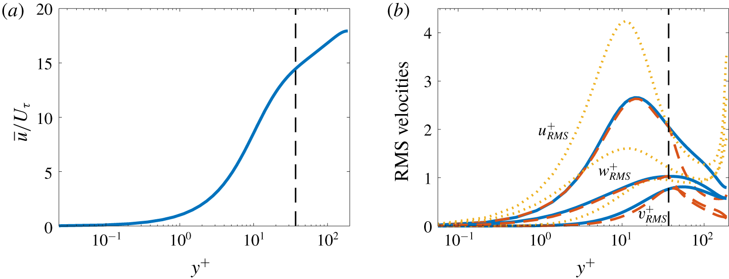
 $p$ is the pressure disturbance. The mean streamwise velocity is computed from the DNS data and is shown in figure 7(a).
(a) Mean and (b) root-mean-squared velocities. Solid lines: true values calculated from the DNS data. Dashed lines: estimates obtained from the model using measurements at  $y^{+}=37$ (
 $y/h=0.2$). Dotted lines: estimates based on a white noise assumption. The input location is demarcated in the figure by the vertical dashed line.

Following previous work (Reynolds & Hussain Reference Reynolds and Hussain1972; del Álamo & Jiménez Reference del Álamo and Jiménez2006; Hwang & Cossu Reference Hwang and Cossu2010; Moarref & Jovanović Reference Moarref and Jovanović2012; Illingworth, Monty & Marusic Reference Illingworth, Monty and Marusic2018), we have included an eddy viscosity model in the form of the total viscosity function  $\unicode[STIX]{x1D708}_{T}(y)$. These references and others have shown that including an eddy viscosity substantially improves the predictive capabilities of linearized models of the Navier–Stokes equations for wall-bounded flows, and recent work has shown similar benefits for free-shear flows (Pickering et al. Reference Pickering, Rigas, Sipp, Schmidt and Colonius2019). Of particular relevance, Morra et al. (Reference Morra, Semeraro, Henningson and Cossu2019) recently showed that improved predictions of the statistics of a turbulent channel flow can be obtained by including an eddy viscosity for a resolvent model forced by white noise. By including an eddy viscosity in our method, we automatically inherit this improvement, while also using data to obtain an improved estimate of the forcing compared to a white noise assumption. Details of our eddy viscosity formulation are consistent with those of Illingworth et al. (Reference Illingworth, Monty and Marusic2018) and can be found there.
Since the linearized equations are homogeneous in  $x$ and
 $z$, we can apply Fourier transforms in these directions and obtain an equation for each
 $(k_{x},k_{z})$ wavenumber pair in the form of equation (2.7) with
 $$\begin{eqnarray}{\mathcal{A}}=\text{i}k_{x}A_{x}+A_{y}\frac{\unicode[STIX]{x2202}}{\unicode[STIX]{x2202}y}+\text{i}k_{z}A_{z}-k_{x}^{2}A_{xx}+A_{yy}\frac{\unicode[STIX]{x2202}^{2}}{\unicode[STIX]{x2202}y^{2}}-k_{z}^{2}A_{zz},\end{eqnarray}$$
 ${\mathcal{G}}=\text{diag}([1,1,1,0])$ and
 $\boldsymbol{q}=[u,v,w,p]^{\text{T}}$. The matrices in (3.8) are provided in appendix B. The wall-normal direction
 $y$ is discretized using 201 Chebyshev polynomials, and no-slip boundary conditions are applied at the walls.
We choose the known quantity  $\boldsymbol{y}$ to be the three velocity components at
 $y/h=0.2$, which in inner units corresponds to
 $y^{+}=37$. This is the same
 $y/h$ value considered by Illingworth et al. (Reference Illingworth, Monty and Marusic2018) in their recent Kalman filter study, although the
 $y^{+}$ value is different due to differing Reynolds numbers.
To visualize the results, we will focus on the velocity energy spectra, which are obtained from the cross-spectral density tensor as
 $$\begin{eqnarray}\unicode[STIX]{x1D640}_{\boldsymbol{q}\boldsymbol{q}}(y;k_{x},k_{z},\unicode[STIX]{x1D714})=\unicode[STIX]{x1D64E}_{\boldsymbol{q}\boldsymbol{q}}(y,y;k_{x},k_{z},\unicode[STIX]{x1D714}).\end{eqnarray}$$
3.2.3 Root-mean-squared velocities
We begin by examining the root-mean-squared (r.m.s.) velocity fluctuations, which are obtained by integrating  $\unicode[STIX]{x1D640}_{\boldsymbol{q}\boldsymbol{q}}(y;k_{x},k_{z},\unicode[STIX]{x1D714})$ in
 $k_{x}$,
 $k_{z}$ and
 $\unicode[STIX]{x1D714}$ and taking the square root. The true r.m.s. velocity fluctuations computed from the DNS data and those obtained from the model are compared in figure 7(b) as a function of
 $y^{+}$. The r.m.s. values are accurately estimated for all three velocity components in the near-wall region, specifically for
 $y^{+}\lesssim 45$ (
 $y/h\lesssim 0.25$). The streamwise and spanwise velocity estimates are especially accurate, while slightly larger discrepancies are observed for the wall-normal velocity. Notably, the model accurately captures both the location and magnitude of the
 $u_{rms}$ peak. For larger values of
 $y^{+}$, the r.m.s. values quickly fall below the DNS values. Results in the following section show that this under prediction is primarily due to missing energy at small scales, which do not have a footprint at the probe location. This missing energy could potentially be recovered by appropriate modelling of the
 $\boldsymbol{E}_{ij}$ terms that have been set to zero, as discussed in § 4.
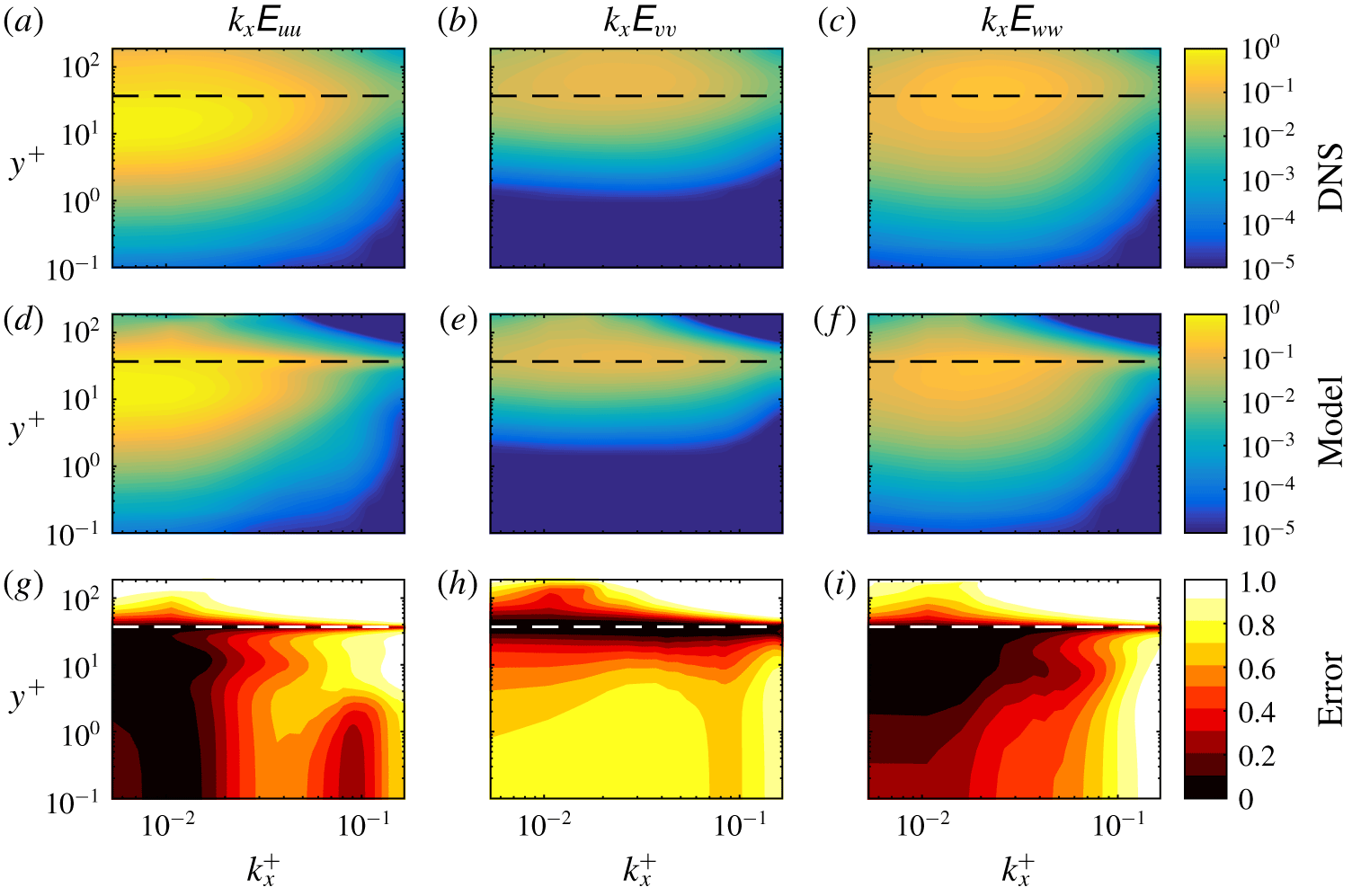
Premultiplied energy spectra as a function of streamwise wavenumber  $k_{x}^{+}$ and wall-normal distance
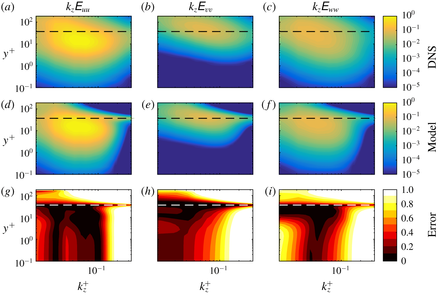
 $y^{+}$. (a–c) DNS. (d–f) Estimates from the model. (g–i) Error metric defined by (3.10). Columns from left to right: streamwise velocity, wall-normal velocity, spanwise velocity. The horizontal dashed lines show the location of the known input data,
 $y^{+}=37$.

Premultiplied energy spectra as a function of spanwise wavenumber  $k_{z}^{+}$ and wall-normal distance
 $y^{+}$. Details are the same as figure 8.

We also show in this figure results obtained by assuming a spatially uncorrelated forcing of the form  $\unicode[STIX]{x1D64E}_{\boldsymbol{f}\boldsymbol{f}}=p(\unicode[STIX]{x1D714})\unicode[STIX]{x1D644}$, as in Morra et al. (Reference Morra, Semeraro, Henningson and Cossu2019). This is similar to a classical white noise model (Farrell & Ioannou Reference Farrell and Ioannou1993; Jovanović & Bamieh Reference Jovanović and Bamieh2001), except that the amplitude of the forcing at each frequency is determined by matching the PSD of the streamwise velocity. The estimated r.m.s. values are less accurate over most of the channel, and still worse results (not shown) are obtained using a true white noise assumption (
 $p(\unicode[STIX]{x1D714})=p_{0}$). These results demonstrate that the resolvent-based estimation method leads to an improved estimate of the nonlinear forcing and resulting flow statistics compared to models based on assumptions of white noise and spatially uncorrelated forcing. Accordingly, we do not further consider these model in what follows and focus solely on results from our resolvent-based estimation method.
3.2.4 Energy spectra
Figures 8–10 show the energy spectrum for each velocity component as a function of  $y^{+}$ and
 $k_{x}^{+}$,
 $k_{z}^{+}$, and
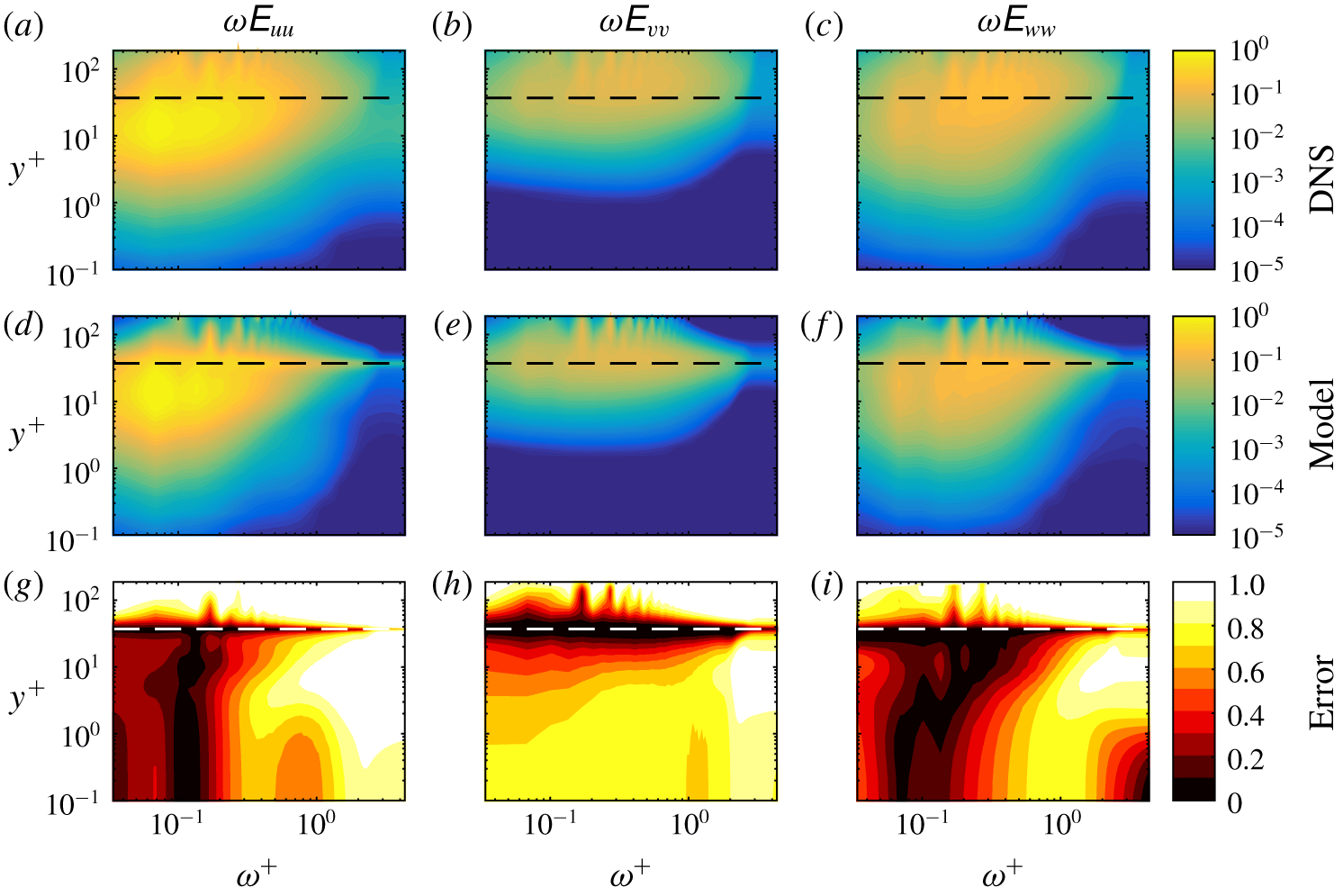
 $\unicode[STIX]{x1D714}^{+}$, respectively. In each case, the energy has been integrated over the other two Fourier variables. The energies have been premultiplied by the appropriate wavenumber or frequency to account for the logarithmic axes in wave space. The contour levels are logarithmically spaced and span five orders of magnitude, with the highest level equal to the maximum value of the DNS streamwise velocity spectrum. The same levels are used in all subplots so that magnitudes can be directly compared. The true spectra computed from the DNS data appear in the top row of each figure, and the corresponding model estimates appear in the second row. The error of the estimate is quantified by the metric
 $$\begin{eqnarray}\frac{|\tilde{\unicode[STIX]{x1D640}}_{\boldsymbol{q}\boldsymbol{q}}-\unicode[STIX]{x1D640}_{\boldsymbol{q}\boldsymbol{q}}|}{\unicode[STIX]{x1D640}_{\boldsymbol{q}\boldsymbol{q}}},\end{eqnarray}$$
which is shown in the third row of each figure.
Premultiplied energy spectra as a function of frequency  $\unicode[STIX]{x1D714}^{+}$ and wall-normal distance
 $y^{+}$. Details are the same as figure 8.

In all cases, the model captures the energy distribution of all three velocity components with reasonable accuracy for  $y^{+}\lesssim 45$, except at the highest wavenumbers and frequencies. As was the case for the r.m.s., the wall-normal velocity is the least accurately predicted. The amplitudes and locations of the energy peaks in
 $(y^{+},k_{x}^{+},k_{z}^{+},\unicode[STIX]{x1D714}^{+})$ space are well captured by the model. On the other hand, the model under-predicts the energy at all wavenumbers and frequencies for higher values of
 $y^{+}$. The highest wavenumbers and frequencies are correctly predicted only near the position of the known input data at
 $y^{+}=37$ (horizontal dashed lines in the figures). This observation can be explained by the smaller wall-normal footprint of smaller scale motions. A small scale eddy detected by the probe will impact the flow only close to the probe location. Similarly, a small scale eddy away from the probe location will not be detected at all. As a result, small scales can only be detected near the probe, leading to accurate predictions near the probe, but significant under predictions of small scale energy away from the probe.
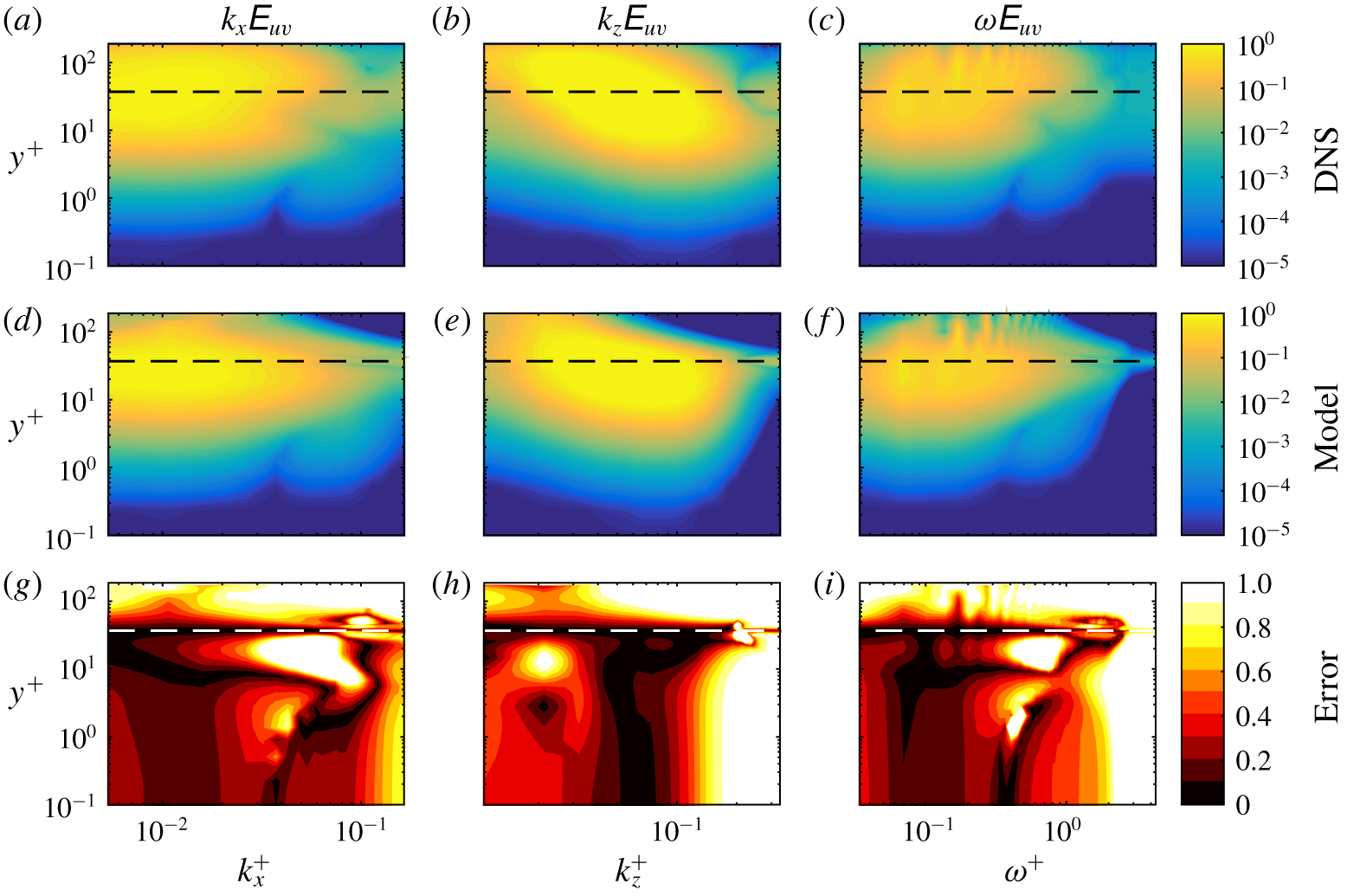
The resolvent-based estimation method also provides estimates of cross-power-spectral densities such as the  $uv$ Reynolds stress
 $E_{uv}$, which is shown as a function of
 $k_{x}$,
 $k_{z}$, and
 $\unicode[STIX]{x1D714}$ in figure 11. Again, accurate results are obtained for low and moderate wavenumbers and frequencies, with a significant under prediction for smaller scales except near the probe.
Premultiplied energy spectra of the  $uv$ Reynolds stresses. (a–c) DNS. (d–f) Estimates from the model. (g–i) Error metric defined in (3.10). Columns from left to right:
 $k_{x}$ wavenumber spectra,
 $k_{z}$ wavenumber spectra, frequency spectra. The horizontal dashed lines show the location of the known input data,
 $y^{+}=37$.

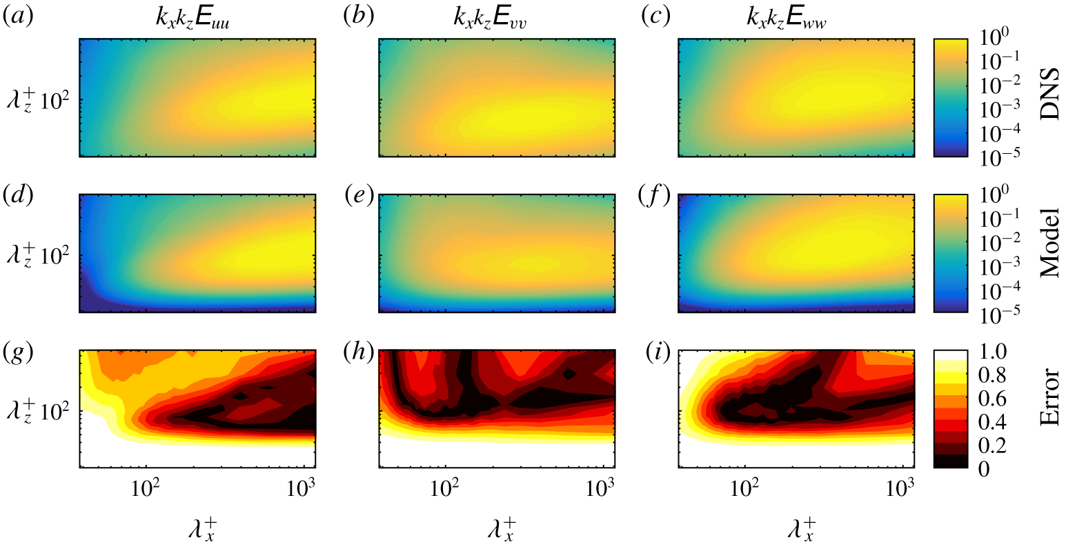
Premultiplied energy spectra as a function of streamwise wavelength  $\unicode[STIX]{x1D706}_{x}^{+}$ and spanwise wavelength
 $\unicode[STIX]{x1D706}_{z}^{+}$. (a–c) DNS. (d–f) Estimates from the model. (g–i) Error as defined by (3.10). Columns from left to right: streamwise velocity, wall-normal velocity, spanwise velocity.

The ability of the resolvent-based estimation method to capture various scales can be further assessed by examining the power spectra as a function of both streamwise and spanwise length scales. Figure 12 shows power spectra as a function of the wavelengths  $\unicode[STIX]{x1D706}_{x}^{+}$ and
 $\unicode[STIX]{x1D706}_{z}^{+}$ at the fixed wall-normal position
 $y^{+}=9$. These wavelengths are related to the previous considered wavenumbers as
 $\unicode[STIX]{x1D706}_{x,z}^{+}=2\unicode[STIX]{x03C0}/k_{x,z}^{+}$. The estimates are accurate for large scales as seen previously, with especially low errors near the energy peak for each velocity component. McKeon & Sharma (Reference McKeon and Sharma2010) showed that these high-energy wavelength pairs are well approximated by the leading few modes of the resolvent operator, which partially explains the success of the resolvent-based estimated method there. Figure 12 also highlights that the energy is most severely under predicted for small spanwise length scales. These results also reinforce the observation from previous works (Encinar et al. Reference Encinar, Lozano-Durén and Jiménez2018) that detached fluid motions far from the wall are not correctly captured by linear models, probably because their limited wall-normal extent does not allow for their full reconstruction.
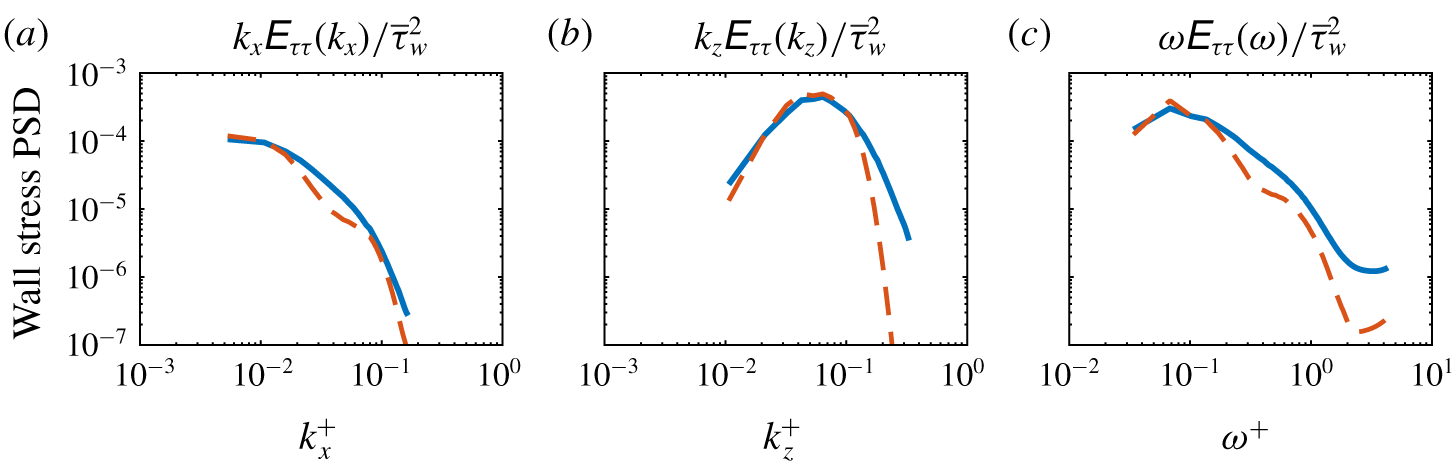
Premultiplied energy spectra of wall shear stress stresses. Solid lines: DNS. Dashed lines: estimates from the model. Columns from left to right:  $k_{x}$ wavenumber spectra,
 $k_{z}$ wavenumber spectra, frequency spectra.

One key quantity for which estimates may be of interest is the wall shear stress, especially for future developments in the context of wall-modelled large-eddy simulation. Figure 13 shows premultiplied spectra of the streamwise wall shear stress as a function of  $k_{x}^{+}$,
 $k_{z}^{+}$, and
 $\unicode[STIX]{x1D714}^{+}$. The estimates are accurate for low and moderate wavenumbers and frequency, with the largest errors observed for high spanwise wavenumbers. The error of the total (integrated) wall shear stress power is 8 %.
3.2.5 Cross-spectra
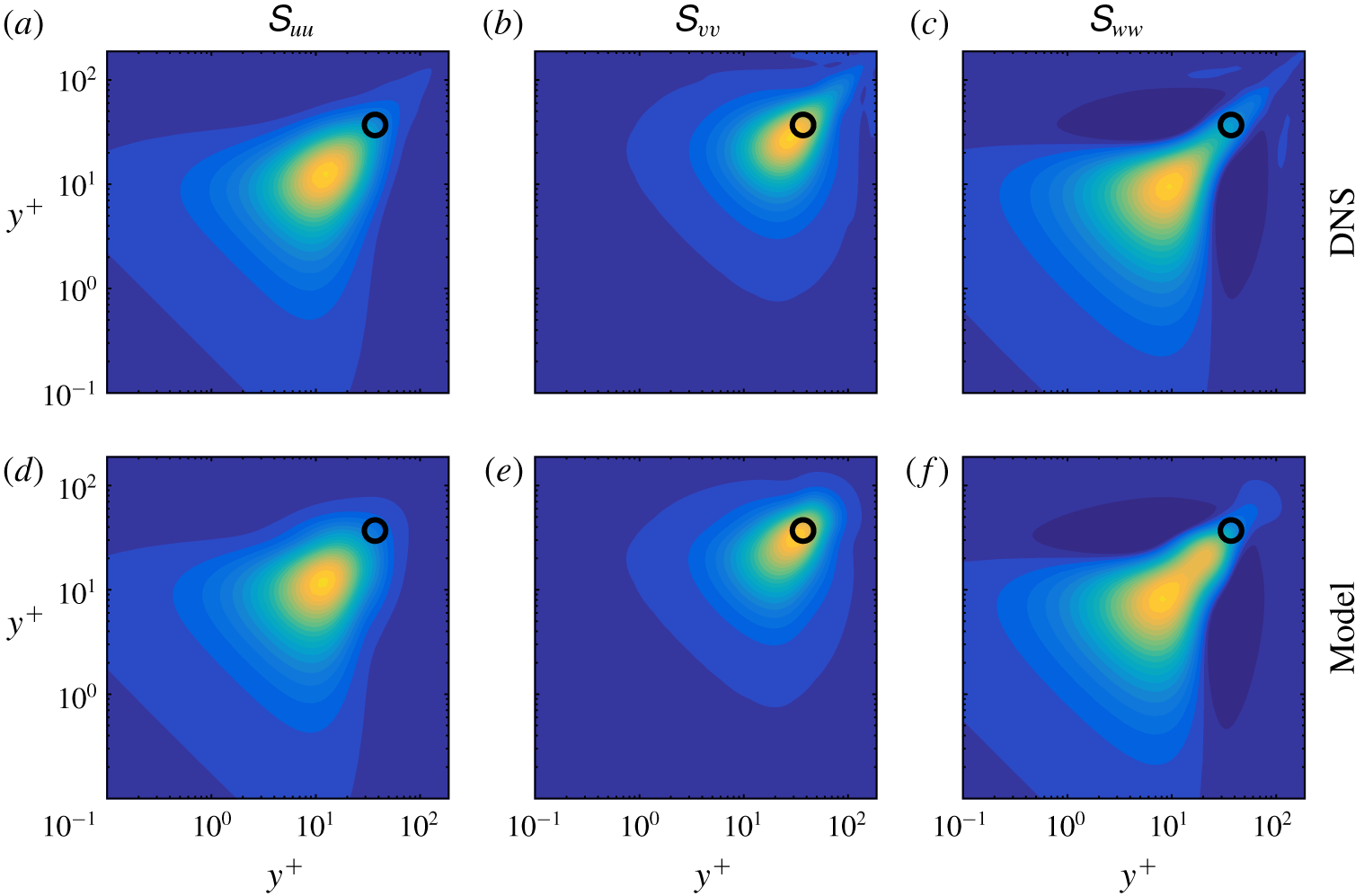
In addition to the energy spectra considered so far, the model also provides predictions for cross-spectra. An example is shown in figure 14. The CSD is plotted as a function of  $y^{+}$ and
 $(y^{+})^{\prime }$ for the streamwise and spanwise wavenumbers
 $\unicode[STIX]{x1D706}_{x}^{+}=700$ and
 $\unicode[STIX]{x1D706}_{z}^{+}=100$, respectively, and the phase speed
 $c_{p}=10$, which are typical values at which coherent structures are expected to appear (Sharma & McKeon Reference Sharma and McKeon2013). The model uses the input data indicated by the black circles, and accurately reproduces the CSD for all three velocity components. Since coherent structures are closely related to the CSD tensor (Towne et al. Reference Towne, Schmidt and Colonius2018), the accuracy of the CSD estimates suggests that the influence of the dominant coherent structures has been captured by the resolvent-based estimation method.
Cross-spectral density for the spectral parameters  $\unicode[STIX]{x1D706}_{x}^{+}\approx 700$,
 $\unicode[STIX]{x1D706}_{z}^{+}\approx 100$ and
 $c_{p}\approx 10$. (a–c) DNS. (d–f) Estimates obtained from the model. Columns from left to right: streamwise, wall-normal and spanwise velocity, respectively. The black circle shows the input location where the DNS data are provided to the model.

3.2.6 Autocorrelations and convection velocity
Next, we consider the space–time correlations
 $$\begin{eqnarray}\unicode[STIX]{x1D63E}_{\boldsymbol{q}\boldsymbol{q}}(y,y^{\prime },\unicode[STIX]{x1D6FF}x,\unicode[STIX]{x1D6FF}z,\unicode[STIX]{x1D6FF}t)=E\{\boldsymbol{q}(x,y,z,t)\boldsymbol{q}^{\ast }(x+\unicode[STIX]{x1D6FF}x,y^{\prime },z+\unicode[STIX]{x1D6FF}z,t+\unicode[STIX]{x1D6FF}t)\},\end{eqnarray}$$
where the expectation is taken over all  $x$,
 $z$ and
 $t$. These correlations can be recovered from the cross-spectra discussed so far by taking inverse Fourier transforms,
 $$\begin{eqnarray}\unicode[STIX]{x1D63E}_{\boldsymbol{q}\boldsymbol{q}}(y,y^{\prime },\unicode[STIX]{x1D6FF}x,\unicode[STIX]{x1D6FF}z,\unicode[STIX]{x1D6FF}t)=\frac{1}{(2\unicode[STIX]{x03C0})^{3}}\int _{-\infty }^{\infty }\int _{-\infty }^{\infty }\int _{-\infty }^{\infty }\unicode[STIX]{x1D64E}_{\boldsymbol{q}\boldsymbol{q}}(y,y^{\prime },k_{x},k_{z},\unicode[STIX]{x1D714})\text{e}^{\text{i}k_{x}\unicode[STIX]{x1D6FF}x}\text{e}^{\text{i}k_{z}\unicode[STIX]{x1D6FF}z}\text{e}^{\text{i}\unicode[STIX]{x1D714}\unicode[STIX]{x1D6FF}t}\,\text{d}k_{x}\,\text{d}k_{z}\,\text{d}\unicode[STIX]{x1D714}.\end{eqnarray}$$
We will focus on the autocorrelations
 $$\begin{eqnarray}\unicode[STIX]{x1D64D}_{\boldsymbol{q}\boldsymbol{q}}(y;\unicode[STIX]{x1D6FF}x,\unicode[STIX]{x1D6FF}z,\unicode[STIX]{x1D6FF}t)=\unicode[STIX]{x1D63E}_{\boldsymbol{q}\boldsymbol{q}}(y,y,\unicode[STIX]{x1D6FF}x,\unicode[STIX]{x1D6FF}z,\unicode[STIX]{x1D6FF}t).\end{eqnarray}$$
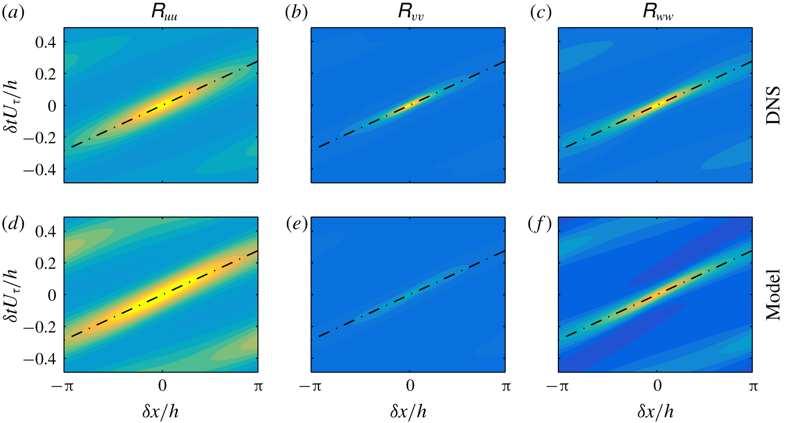
Autocorrelation as a function of streamwise separation  $\unicode[STIX]{x1D6FF}x$ and temporal separation
 $\unicode[STIX]{x1D6FF}t$ at
 $y^{+}=9$ (
 $y/h=0.05$). (a–c) DNS. (d–f) Estimates obtained from the model. Columns from left to right: streamwise, wall-normal and spanwise velocity, respectively. The contour levels are linearly spaced between
 $90\,\%$ and
 $-20\,\%$ of the maximum value of the DNS autocorrelation of each velocity component. The slope of the dashed lines gives the inverse of the dominant convection velocity.

As an example, we examine the autocorrelations as a function of the streamwise and temporal lag variables  $\unicode[STIX]{x1D6FF}x$ and
 $\unicode[STIX]{x1D6FF}t$, respectively, at a fixed wall-normal location
 $y/h=0.05$ (
 $y^{+}=9$). Figure 15 shows the autocorrelation of each velocity component as a function of
 $\unicode[STIX]{x1D6FF}x$ and
 $\unicode[STIX]{x1D6FF}t$, i.e. the space–time autocorrelations along the streamwise direction. The contour levels are logarithmically spaced between the maximum value of the streamwise autocorrelation from DNS and span five orders of magnitude. The same levels are used in all subplots. The inverse slope of the band of high correlation in each plot provides a measure of the convection velocity of disturbances. At this wall-normal location, the convection velocity is approximately
 $11U_{\unicode[STIX]{x1D70F}}$ and is accurately approximated by the estimate for all three velocity components. The correlation magnitudes are also well approximated aside from a moderate under prediction of the peak wall-normal velocity correlations.
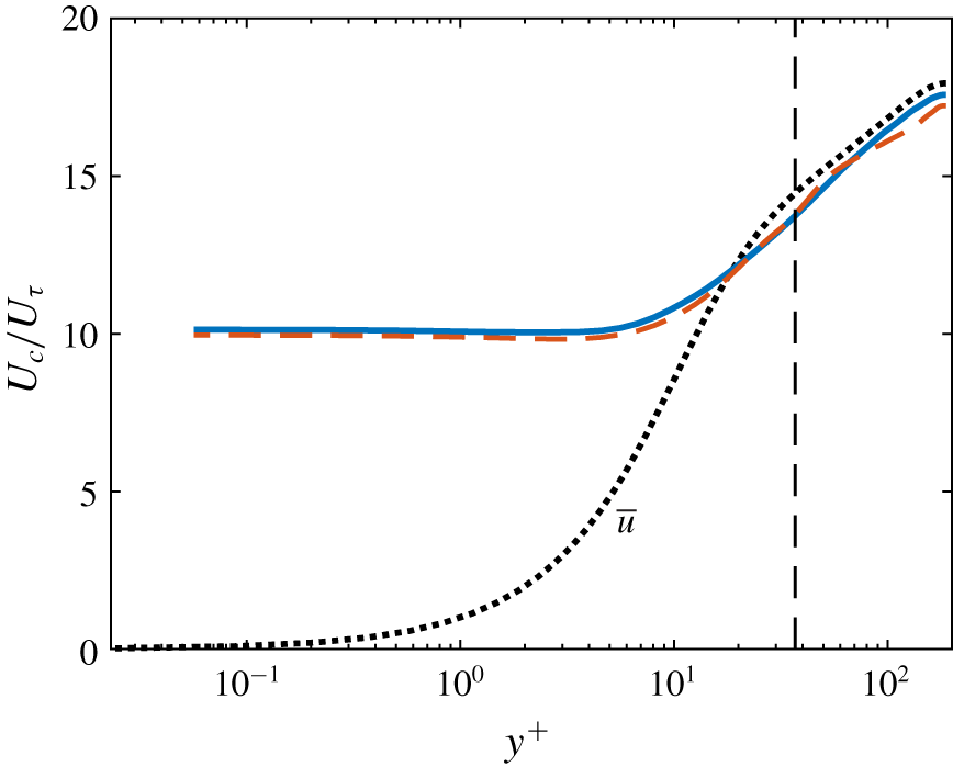
Figure 16 shows the convection velocity calculated from the DNS data and resolvent-based estimates as a function of wall-normal position. Following previous authors (Choi & Moin Reference Choi and Moin1990; Park & Moin Reference Park and Moin2016), the convection velocity is defined as
 $$\begin{eqnarray}U_{c}(y)=\text{arg max}_{U}\int _{-\infty }^{\infty }\unicode[STIX]{x1D619}_{uu}(y,Ut,0,t)\,\text{d}t,\end{eqnarray}$$
i.e. the direction in  $x$–
 $t$ space along which the integrated streamwise velocity correlation is maximum.
Consistent with the observation of Kim & Hussain (Reference Kim and Hussain1993) and del Álamo & Jiménez (Reference del Álamo and Jiménez2009), the convection velocity computed from the DNS data is approximately equal to the mean streamwise velocity for  $y^{+}\gtrsim 10$ and asymptotes to a constant value of about
 $10U_{\unicode[STIX]{x1D70F}}$ near the wall. These trends are accurately captured by convection velocities computed from the estimated autocorrelations. The near-wall asymptotic convection velocity is under predicted by just 1.7 %, and the error in the outer region is less than the difference between the true convection velocity and the mean velocity up to
 $y^{+}\approx 100$.
Convection velocity as a function of  $y^{+}$. Solid lines: true values calculated from the DNS data. Dashed lines: estimates obtained from the model using measurements at
 $y^{+}=37$ (
 $y/h=0.2$). This input location is demarcated in the figure by the vertical dashed line, and the mean velocity profile is shown as a dotted line for reference.

4 Conclusions
Building on the work of Beneddine et al. (Reference Beneddine, Sipp, Arnault, Dandois and Lesshafft2016), Gómez et al. (Reference Gómez, Blackburn, Rudman, Sharma and McKeon2016a) and Zare et al. (Reference Zare, Jovanović and Georgiou2017), this paper introduces a method for estimating space–time flow statistics from a limited set of known values. The method is based on the resolvent methodology developed by McKeon & Sharma (Reference McKeon and Sharma2010) and the statistical interpretation of this theory proposed by Towne et al. (Reference Towne, Schmidt and Colonius2018). The central idea of our approach is to (partially) infer the nonlinear term of the linearized Navier–Stokes equations using limited flow data. This nonlinear term is then used as a forcing acting on the resolvent operator to reconstruct unknown statistics of the flow.
The resolvent-based estimation method was demonstrated using two example problems. First, it was applied to the complex Ginzburg–Landau equation, which serves as a convenient model of a convectively unstable flow. Using input data from three probe locations, the method provided good estimates of the unknown power spectra, cross-spectra and space–time correlations within the energetic regions of  $\unicode[STIX]{x1D714}$-
 $x$ or
 $\unicode[STIX]{x1D70F}$-
 $x$ space. Comparisons were then made with the rank-1 model proposed by Beneddine et al. (Reference Beneddine, Sipp, Arnault, Dandois and Lesshafft2016). The two methods gave similar results when the probes were placed at locations dominated by a single resolvent mode, but the new method gave superior results when the probes were placed at locations that violate this underlying assumption of the rank-1 model. The improved behaviour in this case is important for turbulent flows, which cannot in general be described by a single resolvent mode. Furthermore, the estimates provided by the new method improve with the addition of more known input data and converge in the limit of complete knowledge of the flow, unlike the rank-1 method.
Second, we applied our method to a turbulent channel at friction Reynolds number  $Re_{\unicode[STIX]{x1D70F}}=187$. Using data exclusively from the wall-normal location
 $y/h=0.2$ (
 $y^{+}=37$), the method provides good estimates of the velocity energy spectra and autocorrelations for
 $y\lesssim 0.25$ (
 $y^{+}\lesssim 45$). The energies and autocorrelations are under-predicted further away from the wall due to missing energy at small scales that requires additional modelling to capture. If the success of the model in the near-wall region using knowledge of the interior flow persists at higher Reynolds numbers, it could be useful for designing new wall models for large-eddy simulation that are capable of capturing fluctuations of wall quantities such as shear stress and heat transfer and near-wall velocities that play an important role, for example, in particle laden flows. More broadly, the method could be useful for flow estimation and control – the statistical estimates obtained by our method can be used to obtain real-time flow estimates using approaches such as linear stochastic estimation (Adrian Reference Adrian1994; Bonnet et al. Reference Bonnet, Cole, Delville, Glauser and Ukeiley1994) and
 $H_{1}$ and
 $H_{2}$ frequency response functions (Bendat & Piersol Reference Bendat and Piersol1990; Sasaki et al. Reference Sasaki, Piantanida, Cavalieri and Jordan2017).
Additional work is required to understand the channel flow observations, further assess the impact of the location of the known input data, and determine whether the results described in this paper will extend to higher Reynolds numbers and other types of turbulent flows. The properties and performance of the method should also be directly compared to other approaches that use the linearized flow equations as the basis for flow estimation, including the recent Kalman-filter-based approach described by Illingworth et al. (Reference Illingworth, Monty and Marusic2018).
The method itself could also be further improved by modelling the portions of the forcing cross-spectral density that cannot be observed using the known data. In the current formulation, these terms are simply set to zero, and there exist several possible alternatives. One is to assume that the unobserved forcing is uncorrelated with the observed part and with itself, leading to the approximation
 $$\begin{eqnarray}\unicode[STIX]{x1D64E}_{\boldsymbol{f}\boldsymbol{f}}=[\unicode[STIX]{x1D651}_{1}\,\,\unicode[STIX]{x1D651}_{2}]\left[\begin{array}{@{}cc@{}}\unicode[STIX]{x1D641}_{11} & \mathbf{0}\\ \boldsymbol{ 0} & a\unicode[STIX]{x1D644}\end{array}\right][\unicode[STIX]{x1D651}_{1}\,\,\unicode[STIX]{x1D651}_{2}]^{\ast }.\end{eqnarray}$$
An appropriate value for the scalar amplitude  $a$ could be determined from the amplitudes of the known
 $\unicode[STIX]{x1D641}_{11}$ terms.
Another possibility is to choose the unobservable terms by insisting that the estimated  $\unicode[STIX]{x1D64E}_{\boldsymbol{f}\boldsymbol{f}}$ projects exclusively onto the first
 $n$ singular modes of
 ${\mathcal{R}}_{q}$, where
 $n$ is the number of measurements. In other words, the forcing would be made unique by limiting its influence to the leading modes of
 ${\mathcal{R}}_{q}$. This possibility is similar to a suggestion made by Beneddine et al. (Reference Beneddine, Yegavian, Sipp and Leclaire2017), except here the expansion coefficients are treated as statistical quantities rather than complex scalars. As shown by Towne et al. (Reference Towne, Schmidt and Colonius2018), this statistical treatment removes a fundamental accuracy restriction imposed by treating the expansion coefficients as deterministic scalars and allows for a convergent approximation. While neither of these aforementioned modifications are likely optimal, they highlight the potential for further improvements within the framework of our resolvent-based estimation method.
Acknowledgements
A.T. thanks E. Martini, A. Cavalieri and P. Jordan for fruitful discussion that helped improve this work. A.L.-D. was partially supported by NASA under grant NNX15AU93A and by ONR under grant N00014-16-S-BA10.
Appendix A. Least-squares approximation of forcing
Let us compute the approximation of  $\unicode[STIX]{x1D64E}_{\boldsymbol{f}\boldsymbol{f}}$ obtained using the pseudo-inverse of
 ${\mathcal{R}}_{y}$, which can be written in terms of the SVD (2.13) as
 $$\begin{eqnarray}{\mathcal{R}}_{y}^{+}=\unicode[STIX]{x1D651}_{\boldsymbol{ y}}\unicode[STIX]{x1D72E}_{\boldsymbol{y}}^{+}\unicode[STIX]{x1D650}_{\boldsymbol{y}}^{\ast },\end{eqnarray}$$
where  $\unicode[STIX]{x1D72E}_{\boldsymbol{y}}^{+}=[\unicode[STIX]{x1D72E}_{1}^{-1}\,\,\mathbf{0}]^{\text{T}}$. Applying the pseudo-inverse and its complex conjugate to the left- and right-hand sides of (2.12a), respectively, gives the pseudo-inverse approximation of
 $\boldsymbol{S}_{\boldsymbol{f}\boldsymbol{f}}$,
 $$\begin{eqnarray}\displaystyle \unicode[STIX]{x1D64E}_{\boldsymbol{f}\boldsymbol{f}}^{LS} & = & \displaystyle {\mathcal{R}}_{y}^{+}\unicode[STIX]{x1D64E}_{\boldsymbol{y}\boldsymbol{y}}({\mathcal{R}}_{y}^{+})^{\ast }\end{eqnarray}$$
 $$\begin{eqnarray}\displaystyle & = & \displaystyle \unicode[STIX]{x1D651}_{\boldsymbol{y}}\unicode[STIX]{x1D72E}_{\boldsymbol{y}}^{-1}\unicode[STIX]{x1D650}_{\boldsymbol{y}}^{\ast }\unicode[STIX]{x1D64E}_{\boldsymbol{y}\boldsymbol{y}}\unicode[STIX]{x1D650}_{\boldsymbol{y}}\unicode[STIX]{x1D72E}_{\boldsymbol{y}}^{-1}\unicode[STIX]{x1D651}_{\boldsymbol{y}}^{\ast }\end{eqnarray}$$
 $$\begin{eqnarray}\displaystyle & = & \displaystyle [\unicode[STIX]{x1D651}_{1}\,\,\unicode[STIX]{x1D651}_{2}]\left[\begin{array}{@{}cc@{}}\unicode[STIX]{x1D72E}_{1}^{-1} & \mathbf{0}\end{array}\right]^{T}\unicode[STIX]{x1D650}_{\boldsymbol{y}}^{\ast }\unicode[STIX]{x1D64E}_{\boldsymbol{y}\boldsymbol{y}}\unicode[STIX]{x1D650}_{\boldsymbol{y}}\left[\begin{array}{@{}cc@{}}\unicode[STIX]{x1D72E}_{1}^{-1} & \mathbf{0}\end{array}\right][\unicode[STIX]{x1D651}_{1}\,\,\unicode[STIX]{x1D651}_{2}]^{\ast }\end{eqnarray}$$
 $$\begin{eqnarray}\displaystyle & = & \displaystyle \unicode[STIX]{x1D651}_{1}\unicode[STIX]{x1D72E}_{1}^{-1}\unicode[STIX]{x1D650}_{\boldsymbol{y}}^{\ast }\unicode[STIX]{x1D64E}_{\boldsymbol{y}\boldsymbol{y}}\unicode[STIX]{x1D650}_{\boldsymbol{y}}\unicode[STIX]{x1D72E}_{1}^{-1}\unicode[STIX]{x1D651}_{1}^{\ast }\end{eqnarray}$$
 $$\begin{eqnarray}\displaystyle & = & \displaystyle \unicode[STIX]{x1D651}_{1}\unicode[STIX]{x1D641}_{11}\unicode[STIX]{x1D651}_{1}^{\ast },\end{eqnarray}$$
 $\unicode[STIX]{x1D641}_{11}$ given by (2.16). Equation (A 2e) is identical to (2.17), which shows that setting the unknown
 $\unicode[STIX]{x1D641}_{ij}$ terms to zero is equivalent to a least-squares, pseudo-inverse approximation of
 $\unicode[STIX]{x1D64E}_{\boldsymbol{f}\boldsymbol{f}}$.
Appendix B. Linearized incompressible Navier–Stokes operators
The matrices defining the linearized incompressible Navier–Stokes equations in (2.7) and (3.8) are,
 $$\begin{eqnarray}\unicode[STIX]{x1D63C}_{x}=\left[\begin{array}{@{}cccc@{}}\bar{u} & -\unicode[STIX]{x1D708}_{T}^{\prime } & 0 & 1\\ 0 & \bar{u} & 0 & 0\\ 0 & 0 & \bar{u} & 0\\ 1 & 0 & 0 & \bar{u}\end{array}\right],\quad \unicode[STIX]{x1D63C}_{y}=\left[\begin{array}{@{}cccc@{}}-\unicode[STIX]{x1D708}_{T}^{\prime } & 0 & 0 & 0\\ 0 & -2\unicode[STIX]{x1D708}_{T}^{\prime } & 0 & 1\\ 0 & 0 & -\unicode[STIX]{x1D708}_{T}^{\prime } & 0\\ 0 & 1 & 0 & 0\end{array}\right],\quad \unicode[STIX]{x1D63C}_{z}=\left[\begin{array}{@{}cccc@{}}0 & 0 & 0 & 0\\ 0 & 0 & 0 & 0\\ 0 & -\unicode[STIX]{x1D708}_{T}^{\prime } & 0 & 1\\ 0 & 0 & 1 & 0\end{array}\right],\end{eqnarray}$$
 $$\begin{eqnarray}\unicode[STIX]{x1D63C}_{0}=\left[\begin{array}{@{}cccc@{}}0 & {\displaystyle \frac{\unicode[STIX]{x2202}\bar{u}}{\unicode[STIX]{x2202}y}} & 0 & 0\\ 0 & 0 & 0 & 0\\ 0 & 0 & 0 & 0\\ 0 & 0 & 0 & 0\end{array}\right],\quad {\mathcal{G}}=\left[\begin{array}{@{}cccc@{}}1 & 0 & 0 & 0\\ 0 & 1 & 0 & 0\\ 0 & 0 & 1 & 0\\ 0 & 0 & 0 & 0\end{array}\right],\quad \unicode[STIX]{x1D63D}=\left[\begin{array}{@{}ccc@{}}1 & 0 & 0\\ 0 & 1 & 0\\ 0 & 0 & 1\\ 0 & 0 & 0\end{array}\right],\end{eqnarray}$$
and  $\unicode[STIX]{x1D63C}_{xx}=\unicode[STIX]{x1D63C}_{yy}=\unicode[STIX]{x1D63C}_{zz}=-(1/Re_{\unicode[STIX]{x1D70F}})(\unicode[STIX]{x1D708}_{T}/\unicode[STIX]{x1D708}){\mathcal{G}}$. We have defined
 $\unicode[STIX]{x1D708}_{T}^{\prime }=(1/Re_{\unicode[STIX]{x1D70F}})(1/\unicode[STIX]{x1D708})(\unicode[STIX]{x2202}\unicode[STIX]{x1D708}_{T}/\unicode[STIX]{x2202}y)$.