






1 Introduction
Micro-textured surfaces provide one of the oldest and most investigated methods of skin-friction drag reduction in wall-bounded turbulent flows (Bushnell & Hefner Reference Bushnell, Hefner, Bushnell and Hefner1990). In earliest implementations, arrays of longitudinal microgrooves known as riblets, inspired by the microridges on the shark skin, were embedded in the walls to obtain drag reduction (Walsh Reference Walsh and Hough1980, Reference Walsh1982). Drag reductions of up to
 $10\,\%$
were achieved in laboratory-scale experiments with blade riblets of groove width
 $g^{+0}\equiv gu_{\unicode[STIX]{x1D70F}_{0}}/\unicode[STIX]{x1D708}\approx 17$
, groove depth
 $d/g\approx 0.5$
, and groove spacing
 $w/g\approx 0.02$
(Bechert et al.
Reference Bechert, Bruse, Hage, Van Der Hoeven and Hoppe1997), where
 $g$
,
 $d$
and
 $w$
denote the groove width, depth and spacing, respectively, as shown in figure 1(a), and the
 $+0$
superscript denotes normalization with respect to the kinematic viscosity,
 $\unicode[STIX]{x1D708}$
, and the wall friction velocity,
 $u_{\unicode[STIX]{x1D70F}_{0}}$
, of a ‘base’ turbulent flow with smooth, no-slip walls, at the same bulk Reynolds number as the drag-reduced flow. In full-size applications, however, the drag reductions were more modest, of the order of 5–7 %, due to both the difficulties in employing thin blade riblets in practical applications (Bechert et al.
Reference Bechert, Bruse, Hage, Van Der Hoeven and Hoppe1997), and degradation of drag reduction performance of riblets with increasing Reynolds number, and decreasing friction coefficient, of the ‘base’ flow (Bechert et al.
Reference Bechert, Bruse, Hage, Van Der Hoeven and Hoppe1997; Spalart & McLean Reference Spalart and Mclean2011).
More recently, superhydrophobic (SH) surfaces have received attention as a means of skin-friction drag reduction in turbulent flows (Rothstein Reference Rothstein2010). These are surfaces with apparent receding contact angle exceeding a certain value, e.g.
 $150^{\circ }$
(Schellenberger et al.
Reference Schellenberger, Encinas, Vollmer and Butt2016), in which nano- or micro-structured protrusions on a non-wetting solid surface entrap air underneath the liquid, leading to the so-called Cassie–Baxter state. The entrapped air prevents direct contact between the liquid and the wall, thus providing a mechanism for liquid slip at the walls. Drag reductions of up to 50 % and up to 75 % have been reported in laboratory-scale experiments in turbulent channel flows (Rothstein Reference Rothstein2010) and turbulent boundary layer flows (Park, Sun & Kim Reference Park, Sun and Kim2014), with SH longitudinal microgrooves of size
 $2\lesssim g^{+0}\lesssim 4$
,
 $g/w=1$
and
 $0.8\lesssim g^{+0}\lesssim 1.6$
,
 $g/w=19$
, respectively. Despite these remarkable results in laboratory-scale experiments, SH drag reduction has not yet evolved into a practical means of turbulent skin-friction control, mainly because under the high pressure and high shear rate conditions of turbulent flows in practical environments, the air pockets in the surface micro-texture either collapse (Checco et al.
Reference Checco, Ocko, Rhamn, Black, Tasinkevych, Giacomello and Dietrich2014) or dissolve into the working liquid (Karatay, Tsai & Lammertink Reference Karatay, Tsai and Lammertink2013a
). This has led to the development of more advanced, hierarchical, micro/nano textured surfaces (Feng et al.
Reference Feng, Li, Li, Li, Zhng, Zhai, Song, Liu, Jiang and Zhu2002; Wang et al.
Reference Wang, Koratkar, Ci and Ajayan2007; Kwon et al.
Reference Kwon, Patnakar, Choi and Lee2009; Lee & Kim Reference Lee and Kim2009; Cha et al.
Reference Cha, Yi, Moon, Lee and Kim2010; Lee & Kim Reference Lee and Kim2011) and liquid infused surfaces (Wong et al.
Reference Wong, Kang, Tang, Smythe, Hatton, Grinthal and Aizenberg2011; Rosenberg et al.
Reference Rosenberg, Van Buren, Fu and Smits2016), to enhance the durability and robustness of SH surfaces.
Successful employment of micro-textured surfaces for drag reduction in turbulent flows of practical interest requires an in depth understanding of the mechanism and scaling of drag reduction with micro-textured surfaces, and the pressure and stress loads on the micro-textured surface. This understanding is only beginning to emerge from recent experimental, analytical and computational studies.
(a) Schematic of the channel and the coordinate system; (b) detailed view of the microgroove and the computational grid.
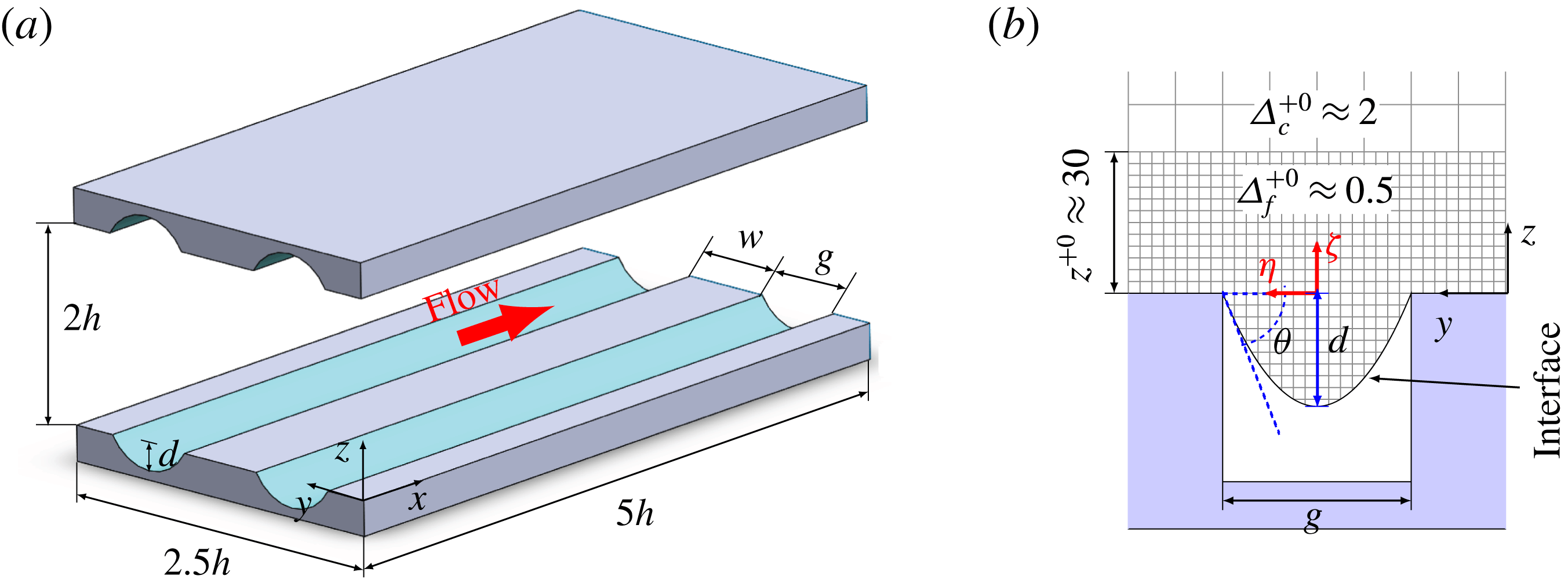
With riblets, it was recognized since the early days that their drag reduction characteristics can be described in terms of the difference,
 $\unicode[STIX]{x0394}h=h_{pl}-h_{pc}$
, between two so-called ‘protrusion heights’,
 $h_{pl}$
and
 $h_{pc}$
, in the longitudinal and cross-flow directions, respectively (Bechert & Bartenwerfer Reference Bechert and Bartenwerfer1989; Luchini, Manzo & Pozzi Reference Luchini, Manzo and Pozzi1991; Bechert et al.
Reference Bechert, Bruse, Hage, Van Der Hoeven and Hoppe1997). These ‘protrusion heights’, which were defined as the distance between the rib tips and the average origin of the velocity profile near the surface, are none other than the ‘slip lengths’ in the streamwise and spanwise directions, defined as
 $L_{s,i}\equiv U_{s,i}/\langle \unicode[STIX]{x2202}\overline{U}_{i}/\unicode[STIX]{x2202}n\rangle |_{wall}$
, where
 $U_{s,i}$
is the average slip velocity in the
 $i$
th direction,
 $n$
is the coordinate normal to the wall, and
 $\langle ~\rangle$
denotes averaging over the pattern of the surface micro-texture. Early studies, however, did not consider that the presence of such a ‘slip length’ in the streamwise direction implies the presence of a streamwise slip velocity, which can directly lead to drag reduction. Instead, they focused on the effect of the protrusion heights,
 $h_{pl}$
and
 $h_{pc}$
, on the dynamics of near-wall turbulence structures (Bechert & Bartenwerfer Reference Bechert and Bartenwerfer1989; Luchini et al.
Reference Luchini, Manzo and Pozzi1991; Bechert et al.
Reference Bechert, Bruse, Hage, Van Der Hoeven and Hoppe1997). Two drag reduction regimes were identified: the ‘viscous regime’, operative at
 $g^{+0}\lesssim 10{-}15$
, for which drag reduction increases almost linearly with increasing groove width; and the ‘breakdown regime’, operative at
 $g^{+0}\gtrsim 15{-}20$
, for which viscous theory breaks down, and drag reduction saturates and begins to diminish with further increases in the groove width, eventually leading to net drag enhancement (Bechert et al.
Reference Bechert, Bruse, Hage, Van Der Hoeven and Hoppe1997). The optimal drag reduction performance was obtained with thin blade riblets of groove width
 $g^{+0}\approx 17$
, for which
 $\unicode[STIX]{x0394}h=h_{pl}-h_{pc}$
was maximized (Bechert et al.
Reference Bechert, Bruse, Hage, Van Der Hoeven and Hoppe1997). More recently, it has been suggested that a better collapse of the drag reduction data in the ‘viscous regime’ can be obtained by parameterizing the magnitude of drag reduction in terms of the square root of the groove cross-sectional area,
 $l_{g}^{+}\equiv \{A_{g}^{+}\}^{1/2}$
, and that the optimal drag reduction performance is achieved at
 $l_{g}^{+}\approx 10.7$
(Garcia-Mayoral & Jimenez Reference Garcia-Mayoral and Jimenez2011a
), where the
 $+$
superscript denotes normalization with respect to the kinematic viscosity,
 $\unicode[STIX]{x1D708}$
, and the wall friction velocity,
 $u_{\unicode[STIX]{x1D70F}}$
, in the flow with micro-textured walls. The drag reduction in the ‘viscous regime’ was attributed to the riblets hampering the cross-flow fluctuating velocity close to the wall, thus providing a resistance to the motion of near-wall streamwise vortical structures (Bechert & Bartenwerfer Reference Bechert and Bartenwerfer1989; Walsh Reference Walsh, Bushnell and Hefner1990; Luchini et al.
Reference Luchini, Manzo and Pozzi1991; Choi, Moin & Kim Reference Choi, Moin and Kim1993; Chu & Karniadakis Reference Chu and Karniadakis1993; Goldstein, Handler & Sirovich Reference Goldstein, Handler and Sirovich1995; Bechert et al.
Reference Bechert, Bruse, Hage, Van Der Hoeven and Hoppe1997). Deterioration of drag reduction in the ‘breakdown regime’ was attributed either to generation of secondary streamwise vorticity over the riblets, due to separation of the cross-flow (Goldstein & Tuan Reference Goldstein and Tuan1998), or to appearance of large-scale spanwise rollers, which develop from a two-dimensional Kelvin–Helmholtz-like instability of the mean streamwise velocity, due to relaxation of the impermeability condition at the wall (Garcia-Mayoral & Jimenez Reference Garcia-Mayoral and Jimenez2011a
). It was not until recently that it was recognized that the presence of a streamwise slip at the plane of riblet tips could by itself lead to drag reduction through augmenting the velocity of the free stream (Garcia-Mayoral & Jimenez Reference Garcia-Mayoral and Jimenez2011a
,Reference Garcia-Mayoral and Jimenez
b
).
With SH surfaces, the earliest direct numerical simulation (DNS) studies investigated the effect of a uniform streamwise or spanwise slip on turbulent skin-friction drag reduction in channel flow. It was shown that uniform streamwise slip leads to drag reduction by augmenting the bulk velocity, while uniform spanwise slip leads to drag enhancement by strengthening the near-wall streamwise vortical structures (Min & Kim Reference Min and Kim2004; Fukagata, Kasagi & Koumoutsakos Reference Fukagata, Kasagi and Koumoutsakos2006). Subsequent DNS studies considered the effect of various micro-patterns of surface slip, such as longitudinal or lateral stripes or tiles, as idealizations of the liquid/gas interfaces in real SH microgrooves or microposts with flat, shear-free boundaries (Martel, Perot & Rothstein Reference Martel, Perot and Rothstein2009; Martel, Rothstein & Perot Reference Martel, Rothstein and Perot2010; Rastegari & Akhavan Reference Rastegari and Akhavan2013; Park, Park & Kim Reference Park, Park and Kim2013; Jelly, Jung & Zaki Reference Jelly, Jung and Zaki2014; Türk et al. Reference Türk, Daschiel, Stroh, Hasegawa and Frohnapfel2014; Rastegari & Akhavan Reference Rastegari and Akhavan2015; Seo, Garcia-Mayoral & Mani Reference Seo, Garcia-Mayoral and Mani2015; Jung, Choi & Kim Reference Jung, Choi and Kim2016; Seo & Mani Reference Seo and Mani2016). Surface slip was shown to be the dominant mechanism of turbulent skin-friction drag reduction with all of these surface micro-patterns, contributing between 80 to 100 % of the overall drag reduction (Rastegari & Akhavan Reference Rastegari and Akhavan2015). Modifications to the turbulence structure and dynamics were shown to contribute no more than 20 % of the total drag reduction with longitudinal microgrooves or microposts of high shear-free fraction, and a drag increase with lateral microgrooves or microposts of moderate shear-free fraction (Rastegari & Akhavan Reference Rastegari and Akhavan2015).
In all of these DNS studies, the liquid/gas interfaces on the SH surfaces were modelled as ‘idealized’, flat, shear-free boundaries. In reality, the liquid/gas interfaces on SH surfaces are not flat, but have a finite curvature (Ou & Rothstein Reference Ou and Rothstein2005; Tsai et al. Reference Tsai, Peters, Pirat, Wessling, Lammertink and Lohse2009; Rathgen & Mugel Reference Rathgen and Mugel2010). Experiments (Steinberger et al. Reference Steinberger, Cottin-Bizonne, Kleimann and Charlaix2007; Tsai et al. Reference Tsai, Peters, Pirat, Wessling, Lammertink and Lohse2009; Karatay et al. Reference Karatay, Haase, Visser, Sun, Lohse, Tsai and Lammertink2013b ), computations (Wang, Teo & Khoo Reference Wang, Teo and Khoo2014) and analytical studies (Sbragaglia & Prosperetti Reference Sbragaglia and Prosperetti2007; Crowdy Reference Crowdy2016) in laminar flow have shown that this interface curvature can affect the slip length and drag reduction by negligible to significant amounts, depending on the size, geometry and orientation of the surface micro-texture relative to the flow, and whether the protrusion angle is positive or negative. In turbulent flow, however, no similar studies of the effect of interface curvature on SH drag reduction have yet been reported.
In this study, we report a first DNS investigation of the effect of interface curvature on turbulent skin-friction drag reduction with SH longitudinal microgrooves in channel flow. The liquid/gas interfaces in the SH microgrooves were modelled as stationary, curved, shear-free boundaries, with the shape of the meniscus determined from the solution of the Young–Laplace equation. This formulation does not allow the collapse or dissolving of the air pockets in the surface micro-texture. Thus the full range of negative protrusion angles, ranging from
 $0$
to
 $-90^{\circ }$
, can be investigated. While negative protrusion angles beyond
 $-30^{\circ }$
, corresponding to contact angles greater than
 $120^{\circ }$
, cannot be sustained on smooth SH walls due to theoretical limits (Nishino et al.
Reference Nishino, Meguro, Nakamae, Matsushita and Ueda1999), this limit can be bypassed by using hierarchical, micro/nano-scale SH surfaces (Feng et al.
Reference Feng, Li, Li, Li, Zhng, Zhai, Song, Liu, Jiang and Zhu2002; Wang et al.
Reference Wang, Koratkar, Ci and Ajayan2007; Kwon et al.
Reference Kwon, Patnakar, Choi and Lee2009; Lee & Kim Reference Lee and Kim2009; Cha et al.
Reference Cha, Yi, Moon, Lee and Kim2010; Lee & Kim Reference Lee and Kim2011; Wong et al.
Reference Wong, Kang, Tang, Smythe, Hatton, Grinthal and Aizenberg2011). In anticipation of deployment of such hierarchical SH surfaces in the future, the full range of negative protrusion angles has been investigated in the present study. For comparison, the same geometries as those formed by the air/water interfaces in the SH longitudinal microgroove were also investigated as riblets, with the shear-free condition on the curved SH interfaces replaced with the no-slip boundary condition, to compare the mechanism of drag reduction in the two flows.
The paper is organized as follows. In § 2 the numerical methods and simulation parameters are reviewed. In § 3, an exact analytical expression for the magnitude of drag reduction in channel flows with any SH or no-slip micro-texture on the walls is derived. This expression allows the net drag reduction to be decomposed into its constitutive elements, thus clarifying the contribution of each element to the net drag reduction. In § 4, results from DNS in channel flows with micro-textured walls are used to evaluate the contribution of each of the terms in this analytical expression to the net drag reduction, to clarify the mechanism of drag reduction with SH longitudinal microgrooves and riblets. It will be shown that SH longitudinal microgrooves and riblets share a common mechanism of drag reduction. In § 5, extrapolation of these results to high Reynolds number flows of practical interest is discussed. In § 6, new possibilities for synergistic use of SH surfaces in conjunction with riblets is discussed, to reduce the pressure loads on SH surfaces and enhance their longevity and sustainability in turbulent flow environments. A summary and conclusions are presented in § 7.
2 Numerical methods and simulation parameters
The numerical simulations reported in this study were all performed using standard D3Q19 (3-Dimensional, 19 discrete velocity), single relaxation time lattice Boltzmann methods (Succi Reference Succi2001) with grid embedding (Lagrava et al.
Reference Lagrava, Malaspinas, Latt and Chopard2012), of grid ratio 4:1, employed in the near-wall region, between the domain boundaries and the buffer layer (
 $z^{+0}\approx 30$
), to improve the accuracy of the computations near the micro-textured walls. The resulting grid spacings were
 $\unicode[STIX]{x1D6E5}_{f}^{+0}\approx 0.5$
for
 $z^{+0}\lesssim 30$
, and
 $\unicode[STIX]{x1D6E5}_{c}^{+0}\approx 2$
for
 $z^{+0}\gtrsim 30$
, in all three directions, as shown in figure 1. In turbulent channel flows with smooth no-slip walls, the lattice Boltzmann method can fairly accurately predict the turbulent flow features with uniform grid spacings of
 $\unicode[STIX]{x1D6E5}^{+0}\approx 2$
throughout the channel, as shown by Lammers et al. (Reference Lammers, Beronov, Volkert, Brenner and Durst2006) and discussed in appendix A, § A.2. With micro-textured surfaces, however, the presence of a slip velocity over the surface micro-indentations leads to steep wall-normal gradients of the streamwise velocity on the no-slip tips of the surface micro-texture, as well as strong shear layers between the slip and no-slip regions at the tip of the surface micro-texture. These shear layers persist up to distances of the order of
 $z\sim g$
, but they become weaker with increasing distance from the wall, such that by
 $z^{+0}\gtrsim 30$
they can be properly resolved by the regular lattice Boltzmann grid of size
 $\unicode[STIX]{x1D6E5}^{+0}\approx 2$
, as shown in appendix A, § A.2. The grid-embedding scheme in the present study was employed to resolve these shear layers in the region
 $z^{+0}\lesssim 30$
, as well as the steep wall-normal gradients of the velocity near the tips of the wall micro-texture.
The liquid/gas interfaces in the SH longitudinal microgrooves were modelled as stationary, curved, shear-free boundaries, with the shape of the meniscus determined from an analytical solution (de Gennes, Brochard-Wyart & Quéré Reference de Gennes, Brochard-Wyart and Quéré2002) of the Young–Laplace equation
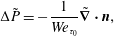 $$\begin{eqnarray}\unicode[STIX]{x0394}\tilde{P}=-\frac{1}{We_{\unicode[STIX]{x1D70F}_{0}}}\tilde{\unicode[STIX]{x1D735}}\boldsymbol{\cdot }\boldsymbol{n},\end{eqnarray}$$
where
 $\unicode[STIX]{x0394}\tilde{P}\equiv \unicode[STIX]{x0394}P/\unicode[STIX]{x1D70C}u_{\unicode[STIX]{x1D70F}_{0}}^{2}$
is the non-dimensional Laplace pressure across the interface,
 $We_{\unicode[STIX]{x1D70F}_{0}}\equiv \unicode[STIX]{x1D70C}u_{\unicode[STIX]{x1D70F}_{0}}^{2}g/\unicode[STIX]{x1D70E}$
is the Weber number,
 $\unicode[STIX]{x1D70C}$
is the fluid density,
 $\unicode[STIX]{x1D70E}$
is the surface tension,
 $\boldsymbol{n}$
is the unit normal to the interface and
 $\tilde{\unicode[STIX]{x1D735}}$
denotes the divergence operator in a non-dimensional local coordinate system,
 $(\tilde{\unicode[STIX]{x1D709}},\tilde{\unicode[STIX]{x1D702}},\tilde{\unicode[STIX]{x1D701}})=(\unicode[STIX]{x1D709},\unicode[STIX]{x1D702},\unicode[STIX]{x1D701})/g$
, centred on the longitudinal microgroove, as shown in figure 1. Integrating (2.1), subject to the boundary conditions
 $\tilde{F}|_{(\tilde{\unicode[STIX]{x1D702}}=\pm 1/2)}=0$
and
 $(\text{d}\tilde{F}/\text{d}\tilde{\unicode[STIX]{x1D702}})|_{(\tilde{\unicode[STIX]{x1D702}}=0)}=0$
, gives the shape of the interface as
 $$\begin{eqnarray}\tilde{F}(\tilde{\unicode[STIX]{x1D702}},\tilde{\unicode[STIX]{x1D705}})=-\frac{1}{2\tilde{\unicode[STIX]{x1D705}}}\left(2\sqrt{1-\tilde{\unicode[STIX]{x1D705}}^{2}\tilde{\unicode[STIX]{x1D702}}^{2}}-\sqrt{4-\tilde{\unicode[STIX]{x1D705}}^{2}}\right),\end{eqnarray}$$
where
 $\tilde{\unicode[STIX]{x1D705}}=(\unicode[STIX]{x0394}\tilde{P}\cdot We_{\unicode[STIX]{x1D70F}_{0}})$
is the non-dimensional curvature of the interface, which is related to the interface protrusion angle through
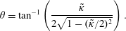 $$\begin{eqnarray}\unicode[STIX]{x1D703}=\tan ^{-1}\left(\frac{\tilde{\unicode[STIX]{x1D705}}}{2\sqrt{1-(\tilde{\unicode[STIX]{x1D705}}/2)^{2}}}\right).\end{eqnarray}$$
Equations (2.2) and (2.3) were used to determine the shape of the interface in the SH longitudinal microgrooves in the present study. Static protrusion angles of
 $\unicode[STIX]{x1D703}=0^{\circ }$
,
 $-30^{\circ }$
,
 $-60^{\circ }$
and
 $-90^{\circ }$
were investigated, covering the full range of protrusion angles from flat interfaces to maximum negative protrusion angle. For comparison, the same geometries as those formed by the menisci of the SH longitudinal microgrooves were also simulated as riblets, with the free-slip boundary condition on the curved interfaces replaced with the no-slip boundary condition.
The boundary conditions on flat no-slip surfaces and flat free-slip interfaces were imposed using half-way bounce back and specular reflection methods (Succi Reference Succi2001), respectively. The boundary conditions on the curved riblet walls were imposed using the so-called ‘central linear interpolation’ (CLI) scheme (Ginzburg, Verhaeghe & d’Humières Reference Ginzburg, Verhaeghe and d’Humières2008). This is a modified version of the half-way bounce back scheme, in which interpolations between pre- and post-collision distribution functions are used to find the unknown distributions at the boundaries while accounting for the full curvature of the wall. The boundary conditions on the curved SH interfaces were imposed using local specular reflection (Ginzburg & Steiner Reference Ginzburg and Steiner2003). In this method, specular reflection is applied locally on the distribution functions in the vicinity of a stepwise realization of the curved interface, to reconstruct the unknown distributions at the boundaries. A number of verification studies were performed to ensure the accuracy of the numerical methods, the adequacy of the grid resolution, and the effect of domain size. These are described in appendix A.
All the simulations reported in the present study were performed in periodic channels of size
 $5h\times 2.5h\times 2h$
in the streamwise (
 $x$
), spanwise (
 $y$
), and wall-normal (
 $z$
) directions, respectively, with SH longitudinal microgrooves or riblets on both walls, as shown in figure 1. For two cases, the simulations were repeated in channels of size
 $20h\times 10h\times 2h$
, as discussed in appendix A, § A.3, to demonstrate the adequacy of the smaller domain size. A constant flow rate was maintained in the channels during the course of all the simulations, corresponding to bulk Reynolds numbers of
 $Re_{b}\equiv q/2\unicode[STIX]{x1D708}=3600$
or
 $Re_{b}=7860$
, where
 $q$
denotes the flow rate per unit spanwise width in the channel. A total of 12 simulations with SH longitudinal microgrooves and 9 simulations with riblets were performed at
 $Re_{b}=3600$
, corresponding to three longitudinal microgrooves of size
 $g^{+0}\approx 14,28,56$
and
 $g/w=7$
, each studied at four protrusion angles of
 $\unicode[STIX]{x1D703}=0^{\circ },-30^{\circ },-60^{\circ },-90^{\circ }$
as SH longitudinal microgrooves, and three protrusion angles of
 $\unicode[STIX]{x1D703}=-30^{\circ },-60^{\circ },-90^{\circ }$
as riblets. In addition, the simulations with SH longitudinal microgrooves of size
 $g^{+0}\approx 14,28$
and
 $g/w=7$
at interface protrusion angle of
 $\unicode[STIX]{x1D703}=-30^{\circ }$
were repeated at
 $Re_{b}=7860$
to assess the effect of the bulk Reynolds number on the drag reduction characteristics. For reference, DNS was also performed in ‘base’ turbulent channel flows with smooth, no-slip walls, at the same bulk Reynolds number as those in the channels with micro-textured walls. The cross-sectional area,
 $A_{0}$
, in the ‘base’ turbulent channel flow was set to the ‘nominal’ cross-sectional area of the channel with micro-textured walls, as defined by area enclosed between the tips of the micro-textures on the opposing walls of the channel. The corresponding friction Reynolds numbers in the ‘base’ turbulent channel flows were
 $Re_{\unicode[STIX]{x1D70F}_{0}}\equiv u_{\unicode[STIX]{x1D70F}_{0}}h/\unicode[STIX]{x1D708}\approx 222$
at
 $Re_{b}=3600$
, and
 $Re_{\unicode[STIX]{x1D70F}_{0}}\approx 442$
at
 $Re_{b}=7860$
. For comparison, all the above simulations were repeated in laminar flow at
 $Re_{b}=150$
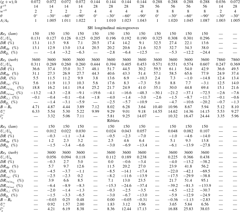
. A summary of all the simulations performed in the present study is given in table 1.
Effective wall slip velocity,
 $DR$
and its decomposition in laminar and turbulent channel flow with SH longitudinal microgrooves or riblets.
3 Drag reduction with micro-textured surfaces in channel flow
Drag reduction with micro-textured surfaces involves contributions from a number of different dynamical effects, some of which are drag reducing, while others are drag enhancing. To clarify the mechanism of drag reduction, these effects need to be separated, so the contribution of each element can be assessed.
For turbulent channel, pipe and plane boundary layer flows with smooth no-slip walls, Fukagata, Iwamoto & Kasagi (Reference Fukagata, Iwamoto and Kasagi2002) derived an analytical expression for the breakdown of the skin-friction coefficient into its constitutive elements. This derivation was later generalized to more geometrically complex no-slip surfaces by Peet & Sagaut (Reference Peet and Sagaut2009). In Rastegari & Akhavan (Reference Rastegari and Akhavan2015), the formulation of Fukagata et al. (Reference Fukagata, Iwamoto and Kasagi2002) was used to derive an analytical expression for the breakdown of drag reduction into its constitutive elements for laminar or turbulent channel flows with any micro-pattern of ‘flat’ SH interfaces. In this section, the formulation of Rastegari & Akhavan (Reference Rastegari and Akhavan2015) will be generalized to channel flows with any three-dimensional SH or riblet micro-texture on the walls.
For steady, fully developed, turbulent channel flow with any SH or riblet micro-texture pattern on the walls, the streamwise Reynolds-averaged momentum equation is given by
 $$\begin{eqnarray}\frac{\unicode[STIX]{x2202}}{\unicode[STIX]{x2202}x}\left(\unicode[STIX]{x1D708}\frac{\unicode[STIX]{x2202}\bar{U}}{\unicode[STIX]{x2202}x}-\overline{uu}-\bar{U}\bar{U}\right)+\frac{\unicode[STIX]{x2202}}{\unicode[STIX]{x2202}y}\left(\unicode[STIX]{x1D708}\frac{\unicode[STIX]{x2202}\bar{U}}{\unicode[STIX]{x2202}y}-\overline{uv}-\bar{U}\bar{V}\right)+\frac{\unicode[STIX]{x2202}}{\unicode[STIX]{x2202}z}\left(\unicode[STIX]{x1D708}\frac{\unicode[STIX]{x2202}\bar{U}}{\unicode[STIX]{x2202}z}-\overline{uw}-\bar{U}\bar{W}\right)=\frac{1}{\unicode[STIX]{x1D70C}}\frac{\unicode[STIX]{x2202}\bar{P}}{\unicode[STIX]{x2202}x},\end{eqnarray}$$
where the overbar denotes Reynolds-averaging;
 $\bar{U}$
,
 $\bar{V}$
,
 $\bar{W}$
and
 $u$
,
 $v$
,
 $w$
are the streamwise (
 $x$
), spanwise (
 $y$
) and wall-normal (
 $z$
) components of the Reynolds-averaged mean and fluctuating velocities, respectively, and
 $\bar{P}$
is the Reynolds-averaged mean pressure. Equation (3.1) can also describe steady, laminar flow in a channel with any SH or riblet micro-texture pattern on the walls if
 $u$
,
 $v$
and
 $w$
are set equal to zero.
Averaging (3.1) over the periodic pattern of the surface micro-texture in the streamwise and spanwise directions, and integrating in the wall-normal direction from the tip of the surface micro-texture, at
 $z=0$
, to a height
 $z$
inside the channel (see figure 1), gives
 $$\begin{eqnarray}\unicode[STIX]{x1D708}\left\langle \frac{\unicode[STIX]{x2202}\bar{U}}{\unicode[STIX]{x2202}z}\right\rangle -\langle \overline{uw}\rangle -\langle \bar{U}\bar{W}\rangle =-\frac{h}{\unicode[STIX]{x1D70C}}\left\langle \frac{\unicode[STIX]{x2202}\bar{P}}{\unicode[STIX]{x2202}x}\right\rangle \left(1-\frac{z}{h}\right),\end{eqnarray}$$
where
 $\langle \,\,\rangle$
denotes averaging in the wall-parallel directions over the periodic pattern of the surface micro-texture;
 $2h$
is the ‘nominal’ full-height of the channel, defined as the distance between the tips of the surface micro-texture on the opposing walls of the channel; and we have used the identity
 $[\unicode[STIX]{x1D708}\langle \unicode[STIX]{x2202}\bar{U}/\unicode[STIX]{x2202}z\rangle -\langle \overline{uw}\rangle -\langle \bar{U}\bar{W}\rangle ]_{z=0}=-\langle \unicode[STIX]{x2202}\overline{P}/\unicode[STIX]{x2202}x\rangle h/\unicode[STIX]{x1D70C}$
, as required by the force balance in the channel between
 $z=0$
and
 $z=2h$
.
Integration of (3.2) in the wall-normal direction, once from 0 to
 $z$
, and again from 0 to
 $h$
(Fukagata et al.
Reference Fukagata, Iwamoto and Kasagi2002; Rastegari & Akhavan Reference Rastegari and Akhavan2015), gives
 $$\begin{eqnarray}-\frac{h}{\unicode[STIX]{x1D70C}U_{b_{0}}^{2}}\left\langle \frac{\unicode[STIX]{x2202}\bar{P}}{\unicode[STIX]{x2202}x}\right\rangle \left(1-3\int _{0}^{1}\left(\frac{-\langle \overline{uw}\rangle -\langle \bar{U}\bar{W}\rangle }{\displaystyle -\frac{h}{\unicode[STIX]{x1D70C}}\left\langle \frac{\unicode[STIX]{x2202}\bar{P}}{\unicode[STIX]{x2202}x}\right\rangle }\right)(1-\unicode[STIX]{x1D712})\,\text{d}\unicode[STIX]{x1D712}\right)=\frac{3}{Re_{b}}\left(1-\frac{Q_{g}}{Q}-\frac{U_{s}}{U_{b_{0}}}\right).\end{eqnarray}$$
Here,
 $U_{b_{0}}$
is the bulk velocity in a smooth, no-slip ‘base’ channel flow with the same bulk Reynolds number,
 $Re_{b}\equiv q/2\unicode[STIX]{x1D708}$
, hence the same flow rate per unit spanwise width,
 $q\equiv Q/L_{y}$
, and the same bulk flow rate,
 $Q$
, as the channel with micro-textured walls, and a ‘base’ channel flow cross-sectional area,
 $A_{0}$
, equal to the ‘nominal’ cross-sectional area of the channel with micro-textured walls, as defined by the area enclosed between the tips of the surface micro-texture on the opposing walls of the channel;
 $Q_{g}$
is the flow rate through the surface micro-texture indentations;
 $U_{s}\equiv \langle \bar{U}\rangle |_{z=0}$
is the average slip velocity at the tip of the surface micro-texture; and
 $\unicode[STIX]{x1D712}\equiv z/h$
is the non-dimensional wall-normal coordinate. Equation (3.3) can be rearranged as
 $$\begin{eqnarray}-\frac{h}{\unicode[STIX]{x1D70C}U_{b_{0}}^{2}}\left\langle \frac{\unicode[STIX]{x2202}\bar{P}}{\unicode[STIX]{x2202}x}\right\rangle =\frac{3}{Re_{b}}\left(1-\frac{Q_{g}}{Q}-\frac{U_{s}}{U_{b_{0}}}\right)\left(\frac{1}{1-3I}\right),\end{eqnarray}$$
where
 $I=I_{\langle \unicode[STIX]{x1D70F}_{R}\rangle }+I_{\langle \unicode[STIX]{x1D70F}_{c}\rangle }=[1/(-\langle \unicode[STIX]{x2202}\bar{P}/\unicode[STIX]{x2202}x\rangle h/\unicode[STIX]{x1D70C})]\int _{0}^{1}(-\langle \overline{uw}\rangle -\langle \bar{U}\bar{W}\rangle )(1-\unicode[STIX]{x1D712})\,\text{d}\unicode[STIX]{x1D712}$
denotes the contribution of the turbulent Reynolds shear stresses,
 $\langle \unicode[STIX]{x1D70F}_{R}\rangle \equiv -\unicode[STIX]{x1D70C}\langle \overline{uw}\rangle$
, and any mean flow shear stresses,
 $\langle \unicode[STIX]{x1D70F}_{c}\rangle \equiv -\unicode[STIX]{x1D70C}\langle \bar{U}\bar{W}\rangle$
, established in the channel due to the presence of the micro-texture on the walls, to the overall wall shear stress, and
 $I$
is bounded by
 $0<I<1/3$
per (3.2). For the ‘base’ channel flow with smooth no-slip walls, (3.4) reduces to
 $$\begin{eqnarray}-\frac{h}{\unicode[STIX]{x1D70C}U_{b_{0}}^{2}}\left\langle \frac{\unicode[STIX]{x2202}\bar{P}}{\unicode[STIX]{x2202}x}\right\rangle _{0}=\frac{3}{Re_{b}}\left(\frac{1}{1-3I_{0}}\right),\end{eqnarray}$$
where
 $I_{0}=I_{\langle \unicode[STIX]{x1D70F}_{R}\rangle _{0}}=[1/(-\langle \unicode[STIX]{x2202}\bar{P}/\unicode[STIX]{x2202}x\rangle _{0}h/\unicode[STIX]{x1D70C})]\int _{0}^{1}-\langle \overline{uw}\rangle _{0}(1-\unicode[STIX]{x1D712})\,\text{d}\unicode[STIX]{x1D712}$
.
Using the definition
 $DR\equiv (1-C_{f}/C_{f_{0}})$
, the magnitude of drag reduction can be expressed as
 $$\begin{eqnarray}DR\equiv \left(1-\frac{C_{f}}{C_{f_{0}}}\right)=\left(1-\frac{\displaystyle \left(\frac{\unicode[STIX]{x1D70F}_{w}}{\unicode[STIX]{x1D70C}(Q/A)^{2}}\right)}{\displaystyle \left(\frac{\unicode[STIX]{x1D70F}_{w_{0}}}{\unicode[STIX]{x1D70C}(Q/A_{0})^{2}}\right)}\right)=\left(1-\frac{\displaystyle \left\langle \frac{\unicode[STIX]{x2202}\bar{P}}{\unicode[STIX]{x2202}x}\right\rangle }{\displaystyle \left\langle \frac{\unicode[STIX]{x2202}\bar{P}}{\unicode[STIX]{x2202}x}\right\rangle _{0}}\left(\frac{A}{A_{0}}\right)^{3}\right),\end{eqnarray}$$
where
 $C_{f}\equiv \unicode[STIX]{x1D70F}_{w}\,/[\unicode[STIX]{x1D70C}(Q/A)^{2}]$
and
 $C_{f_{0}}\equiv \unicode[STIX]{x1D70F}_{w_{0}}/[\unicode[STIX]{x1D70C}(Q/A_{0})^{2}]$
are the skin-friction coefficients,
 $\unicode[STIX]{x1D70F}_{w}$
and
 $\unicode[STIX]{x1D70F}_{w_{0}}$
are the wall shear stresses,
 $A$
and
 $A_{0}$
are the cross-sectional areas, and
 $(Q/A)$
and
 $(Q/A_{0})$
are the bulk velocities, in the channel with micro-textured walls and the ‘base’ channel flow, respectively.
Substitution of (3.4) and (3.5) into (3.6) gives
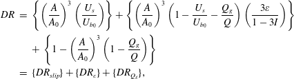 $$\begin{eqnarray}\displaystyle DR & = & \displaystyle \left\{\left(\frac{A}{A_{0}}\right)^{3}\left(\frac{U_{s}}{U_{b_{0}}}\right)\right\}+\left\{\left(\frac{A}{A_{0}}\right)^{3}\left(1-\frac{U_{s}}{U_{b_{0}}}-\frac{Q_{g}}{Q}\right)\left(\frac{3\unicode[STIX]{x1D700}}{1-3I}\right)\right\}\nonumber\\ \displaystyle & & \displaystyle +\,\left\{1-\left(\frac{A}{A_{0}}\right)^{3}\left(1-\frac{Q_{g}}{Q}\right)\right\}\nonumber\\ \displaystyle & = & \displaystyle \{DR_{slip}\}+\{DR_{\unicode[STIX]{x1D700}}\}+\{DR_{Q_{g}}\},\end{eqnarray}$$
where
 $\unicode[STIX]{x1D700}=(I_{0}-I)$
is a measure of the changes in the normalized structure of turbulent Reynolds shear stresses and any mean flow shear stresses developed in the channel due to the presence of the micro-texture on the walls, compared to a ‘base’ channel flow with smooth no-slip walls.
Equation (3.7) provides an exact analytical expression for the magnitude of drag reduction in laminar or turbulent channel flow with any SH or no-slip micro-texture on the walls, while providing a decomposition of drag reduction into: (i) the contributions arising from the effective slip velocity at the wall, represented by
 $\{DR_{slip}\}$
; (ii) the contributions arising from modifications to the structure of turbulent Reynolds shear stresses and any mean flow shear stresses developed in the channel due to the presence of the wall micro-texture, represented by
 $\{DR_{\unicode[STIX]{x1D700}}\}$
; and (iii) the contributions arising from the fraction of the flow rate through the wall micro-texture, represented by
 $\{DR_{Q_{g}}\}$
.
The term
 $\{DR_{\unicode[STIX]{x1D700}}\}$
in (3.7) involves contributions from several different dynamical effects, and can be further decomposed. To begin with, one can decompose
 $\unicode[STIX]{x1D700}=(I_{0}-I)=(I_{\langle \unicode[STIX]{x1D70F}_{R}\rangle _{0}}-I_{\langle \unicode[STIX]{x1D70F}_{R}\rangle }-I_{\langle \unicode[STIX]{x1D70F}_{c}\rangle })$
into
 $$\begin{eqnarray}\unicode[STIX]{x1D700}=\unicode[STIX]{x1D700}_{\langle \unicode[STIX]{x1D70F}_{R}\rangle }+\unicode[STIX]{x1D700}_{\langle \unicode[STIX]{x1D70F}_{c}\rangle },\end{eqnarray}$$
where
 $\unicode[STIX]{x1D700}_{\langle \unicode[STIX]{x1D70F}_{R}\rangle }=(I_{\langle \unicode[STIX]{x1D70F}_{R}\rangle _{0}}-I_{\langle \unicode[STIX]{x1D70F}_{R}\rangle })$
represents the contributions arising from changes in the normalized structure of turbulent Reynolds shear stresses, and
 $\unicode[STIX]{x1D700}_{\langle \unicode[STIX]{x1D70F}_{c}\rangle }=(-I_{\langle \unicode[STIX]{x1D70F}_{c}\rangle })$
represents the contributions arising from changes in the structure of the mean flow shear stresses, due to the presence of the wall micro-texture. Furthermore, the contributions from
 $\unicode[STIX]{x1D700}_{\langle \unicode[STIX]{x1D70F}_{R}\rangle }=(I_{\langle \unicode[STIX]{x1D70F}_{R}\rangle _{0}}-I_{\langle \unicode[STIX]{x1D70F}_{R}\rangle })$
can themselves be decomposed into
 $$\begin{eqnarray}\unicode[STIX]{x1D700}_{\langle \unicode[STIX]{x1D70F}_{R}\rangle }=\unicode[STIX]{x1D700}_{\langle \unicode[STIX]{x1D70F}_{R}\rangle _{Re_{b_{e}}}}+\unicode[STIX]{x1D700}_{\langle \unicode[STIX]{x1D70F}_{R}\rangle _{mod}},\end{eqnarray}$$
where
 $\unicode[STIX]{x1D700}_{\langle \unicode[STIX]{x1D70F}_{R}\rangle _{Re_{b_{e}}}}=(I_{\langle \unicode[STIX]{x1D70F}_{R}\rangle _{0}}-I_{\langle \unicode[STIX]{x1D70F}_{R}\rangle _{Re_{b_{e}}}})$
and
 $\unicode[STIX]{x1D700}_{\langle \unicode[STIX]{x1D70F}_{R}\rangle _{mod}}=(I_{\langle \unicode[STIX]{x1D70F}_{R}\rangle _{Re_{b_{e}}}}-I_{\langle \unicode[STIX]{x1D70F}_{R}\rangle })$
, and
 $I_{\langle \unicode[STIX]{x1D70F}_{R}\rangle _{Re_{b_{e}}}}$
is the value of the
 $I$
integral in a channel flow with smooth no-slip walls at bulk Reynolds number equal to
 $Re_{b_{e}}=(1-U_{s}/U_{b})Re_{b}$
. The decomposition (3.9) is made in consideration of the fact that the presence of an effective slip velocity,
 $U_{s}$
, implies that a fraction,
 $U_{s}/U_{b}$
, of the flow rate can flow inviscidly (Min & Kim Reference Min and Kim2004; Fukagata et al.
Reference Fukagata, Kasagi and Koumoutsakos2006). This reduces the effective bulk Reynolds number of the viscous part of the flow from
 $Re_{b}$
to
 $Re_{b_{e}}=(1-U_{s}/U_{b})Re_{b}$
. As such,
 $\unicode[STIX]{x1D700}_{\langle \unicode[STIX]{x1D70F}_{R}\rangle _{Re_{b_{e}}}}$
represents the changes to the normalized structure of turbulent Reynolds shear stresses in a channel flow with smooth no-slip walls when the bulk velocity,
 $U_{b}$
, is augmented by the presence of an effective wall slip velocity,
 $U_{s}$
, in effect reducing the bulk Reynolds number of the viscous part of the flow from
 $Re_{b}$
to
 $Re_{b_{e}}$
, while
 $\unicode[STIX]{x1D700}_{\langle \unicode[STIX]{x1D70F}_{R}\rangle _{mod}}$
represents the contributions from any other modifications to the normalized structure of the turbulent Reynolds shear stresses due to the presence of the micro-texture on the walls.
The integral
 $I_{\langle \unicode[STIX]{x1D70F}_{R}\rangle _{Re_{b_{e}}}}=[1/(-\langle \unicode[STIX]{x2202}\bar{P}/\unicode[STIX]{x2202}x\rangle _{Re_{b_{e}}}h/\unicode[STIX]{x1D70C})]\int _{0}^{1}-\langle \overline{uw}\rangle _{Re_{b_{e}}}(1-\unicode[STIX]{x1D712})\,\text{d}\unicode[STIX]{x1D712}$
, required for the evaluation of
 $\unicode[STIX]{x1D700}_{\langle \unicode[STIX]{x1D70F}_{R}\rangle _{Re_{b_{e}}}}$
and
 $\unicode[STIX]{x1D700}_{\langle \unicode[STIX]{x1D70F}_{R}\rangle _{mod}}$
, can be computed directly from its definition, by performing additional DNS in smooth no-slip channel flows at bulk Reynolds number equal to
 $Re_{b_{e}}$
. Alternatively,
 $I_{\langle \unicode[STIX]{x1D70F}_{R}\rangle _{Re_{b_{e}}}}$
can be computed by using the relation
 $I_{\langle \unicode[STIX]{x1D70F}_{R}\rangle _{Re_{b_{e}}}}=(1/3)[1-(3/Re_{b_{e}})(U_{b_{e}}/u_{\unicode[STIX]{x1D70F}_{e}})^{2}]$
, which can be obtained from (3.5) for any smooth-wall no-slip turbulent channel flow, where
 $U_{b_{e}}$
and
 $u_{\unicode[STIX]{x1D70F}_{e}}$
represent the bulk velocity and the wall friction velocity, respectively, in a turbulent channel flow at a bulk Reynolds number of
 $Re_{b_{e}}$
. The ratio
 $(U_{b_{e}}/u_{\unicode[STIX]{x1D70F}_{e}})$
can be evaluated from DNS, or from experimental correlations such as Dean’s correlation (Dean Reference Dean1978). In the present study, the integrals
 $I_{\langle \unicode[STIX]{x1D70F}_{R}\rangle _{Re_{b_{e}}}}$
were evaluated by performing additional DNS at bulk Reynolds number equal to
 $Re_{b_{e}}$
.
With these additional decompositions of
 $\{DR_{\unicode[STIX]{x1D700}}\}$
, (3.7) can be written as
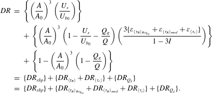 $$\begin{eqnarray}\displaystyle DR & = & \displaystyle \left\{\left(\frac{A}{A_{0}}\right)^{3}\left(\frac{U_{s}}{U_{b_{0}}}\right)\right\}\nonumber\\ \displaystyle & & \displaystyle +\,\left\{\left(\frac{A}{A_{0}}\right)^{3}\left(1-\frac{U_{s}}{U_{b_{0}}}-\frac{Q_{g}}{Q}\right)\left(\frac{3\{\unicode[STIX]{x1D700}_{\langle \unicode[STIX]{x1D70F}_{R}\rangle _{Re_{b_{e}}}}+\unicode[STIX]{x1D700}_{\langle \unicode[STIX]{x1D70F}_{R}\rangle _{mod}}+\unicode[STIX]{x1D700}_{\langle \unicode[STIX]{x1D70F}_{c}\rangle }\}}{1-3I}\right)\right\}\nonumber\\ \displaystyle & & \displaystyle +\,\left\{1-\left(\frac{A}{A_{0}}\right)^{3}\left(1-\frac{Q_{g}}{Q}\right)\right\}\nonumber\\ \displaystyle & = & \displaystyle \{DR_{slip}\}+\{DR_{\langle \unicode[STIX]{x1D70F}_{R}\rangle }+DR_{\langle \unicode[STIX]{x1D70F}_{c}\rangle }\}+\{DR_{Q_{g}}\}\nonumber\\ \displaystyle & = & \displaystyle \{DR_{slip}\}+\{DR_{\langle \unicode[STIX]{x1D70F}_{R}\rangle _{Re_{b_{e}}}}+DR_{\langle \unicode[STIX]{x1D70F}_{R}\rangle _{mod}}+DR_{\langle \unicode[STIX]{x1D70F}_{c}\rangle }\}+\{DR_{Q_{g}}\}.\end{eqnarray}$$
Equation (3.10) shows that the net drag reduction in laminar or turbulent channel flow with any SH or riblet micro-texture pattern on the walls can be decomposed into (i) contributions arising from the effective slip velocity at the wall, represented by
 $\{DR_{slip}\}$
; (ii) contributions arising from modifications to the normalized structure of turbulent Reynolds shear stresses due to augmentation of the bulk velocity by the effective slip velocity at the wall, represented by
 $\{DR_{\langle \unicode[STIX]{x1D70F}_{R}\rangle _{Re_{b_{e}}}}\}$
; (iii) contributions arising from other modifications to the normalized structure of turbulent Reynolds shear stresses due to the presence of the micro-texture on the walls, represented by
 $\{DR_{\langle \unicode[STIX]{x1D70F}_{R}\rangle _{mod}}\}$
; (iv) contributions arising from any mean flow shear stresses developed due to presence of the micro-texture on the walls, represented by
 $\{DR_{\langle \unicode[STIX]{x1D70F}_{c}\rangle }\}$
; and (v) contributions arising from the fraction of the flow rate through the wall micro-texture, represented by
 $\{DR_{Q_{g}}\}$
.
For SH channel flows with ‘idealized’ flat liquid/gas interfaces,
 $(A/A_{0})=1$
and
 $Q_{g}=0$
, and (3.7) or (3.10) reduce to the expression (2.5) given in Rastegari & Akhavan (Reference Rastegari and Akhavan2015). Each of the terms in (3.7) or (3.10) can be evaluated using results from DNS to clarify the mechanism of drag reduction with micro-textured surfaces.
4 Results
4.1 The mechanism of drag reduction with SH longitudinal microgrooves and riblets
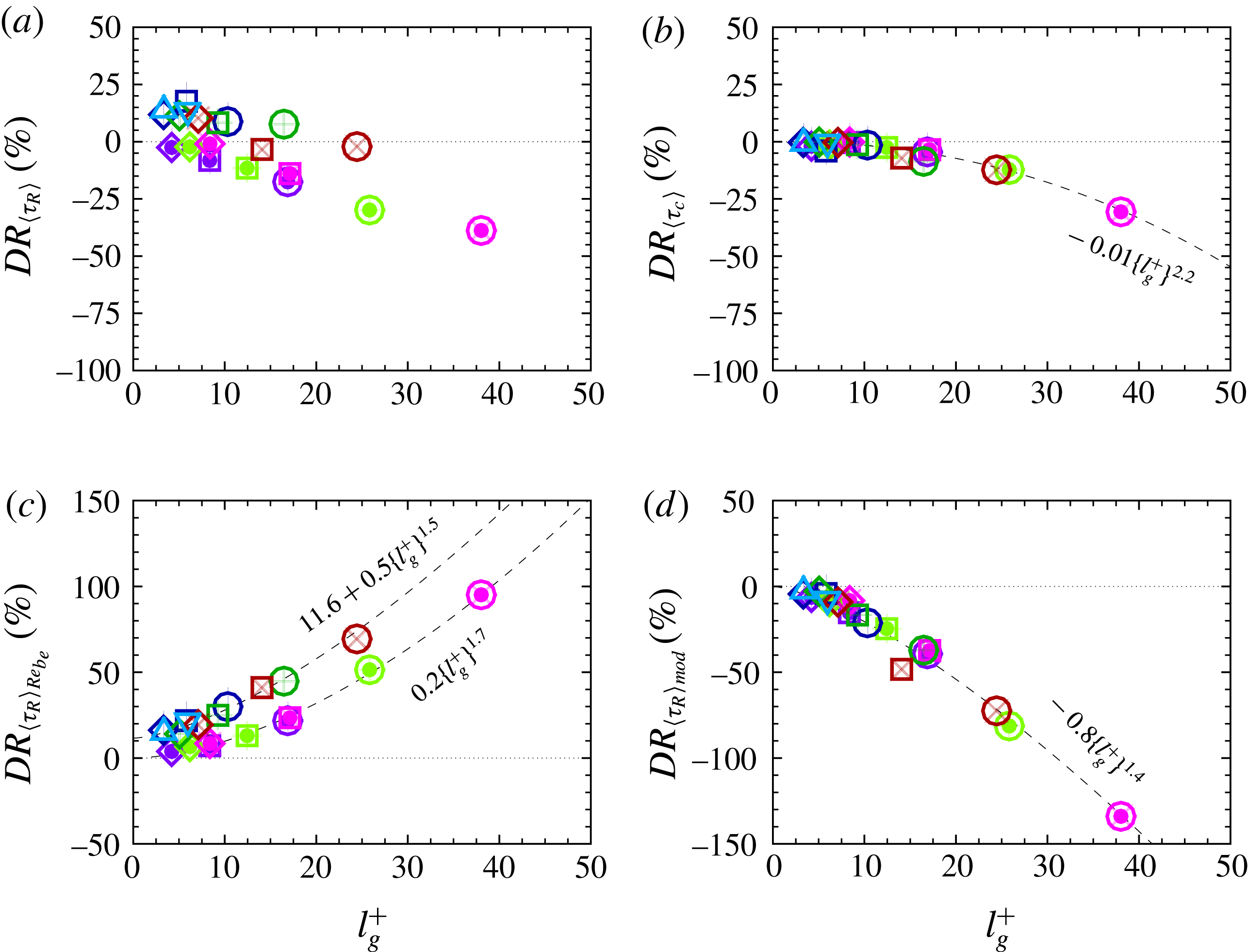
Table 1 and figures 2 and 3 show the wall slip velocities, the magnitudes of
 $DR$
and the decomposition of
 $DR$
into its constitutive elements obtained from DNS of laminar and turbulent channel flows with SH longitudinal microgrooves or riblets in the present study.
Effective wall slip velocity,
 $DR$
and its decomposition into its constitutive elements in (a–c) laminar, and (d–l) turbulent channel flow with SH longitudinal Micro-Grooves (LMGs) or riblets: (a,d,e,f) effective wall slip velocity; (b,g,j)
 $DR$
; (c,h,i,k,l) decomposition of
 $DR$
.


 $Re_{b}=3600$
,
 $\unicode[STIX]{x1D703}=0^{\circ }$
,
 $g^{+0}\approx 14$
, 28, 56;


 $Re_{b}=3600$
,
 $\unicode[STIX]{x1D703}=-30^{\circ }$
,
 $g^{+0}\approx 14$
, 28, 56;


 $Re_{b}=3600$
,
 $\unicode[STIX]{x1D703}=-60^{\circ }$
,
 $g^{+0}\approx 14$
, 28, 56;


 $Re_{b}=3600$
,
 $\unicode[STIX]{x1D703}=-90^{\circ }$
,
 $g^{+0}\approx 14$
, 28, 56;


 $Re_{b}=7860$
,
 $\unicode[STIX]{x1D703}=-30^{\circ }$
,
 $g^{+0}\approx 14$
, 28;


 $Re_{b}=3600$
,
 $\unicode[STIX]{x1D703}=-30^{\circ }$
,
 $g^{+0}\approx 14$
, 28, 56;


 $Re_{b}=3600$
,
 $\unicode[STIX]{x1D703}=-60^{\circ }$
,
 $g^{+0}\approx 14$
, 28, 56;


 $Re_{b}=3600$
,
 $\unicode[STIX]{x1D703}=-90^{\circ }$
,
 $g^{+0}\approx 14$
, 28, 56;
 $\times$
(grey), experimental data of Bechert et al. (Reference Bechert, Bruse, Hage, Van Der Hoeven and Hoppe1997) at
 $5000\leqslant Re_{b}\leqslant 16\,500$
with semi-circular scalloped riblets;
 $\cdots \cdots$
,
 $DR=(U_{s}/U_{b_{0}})(A/A_{0})^{3}$
.
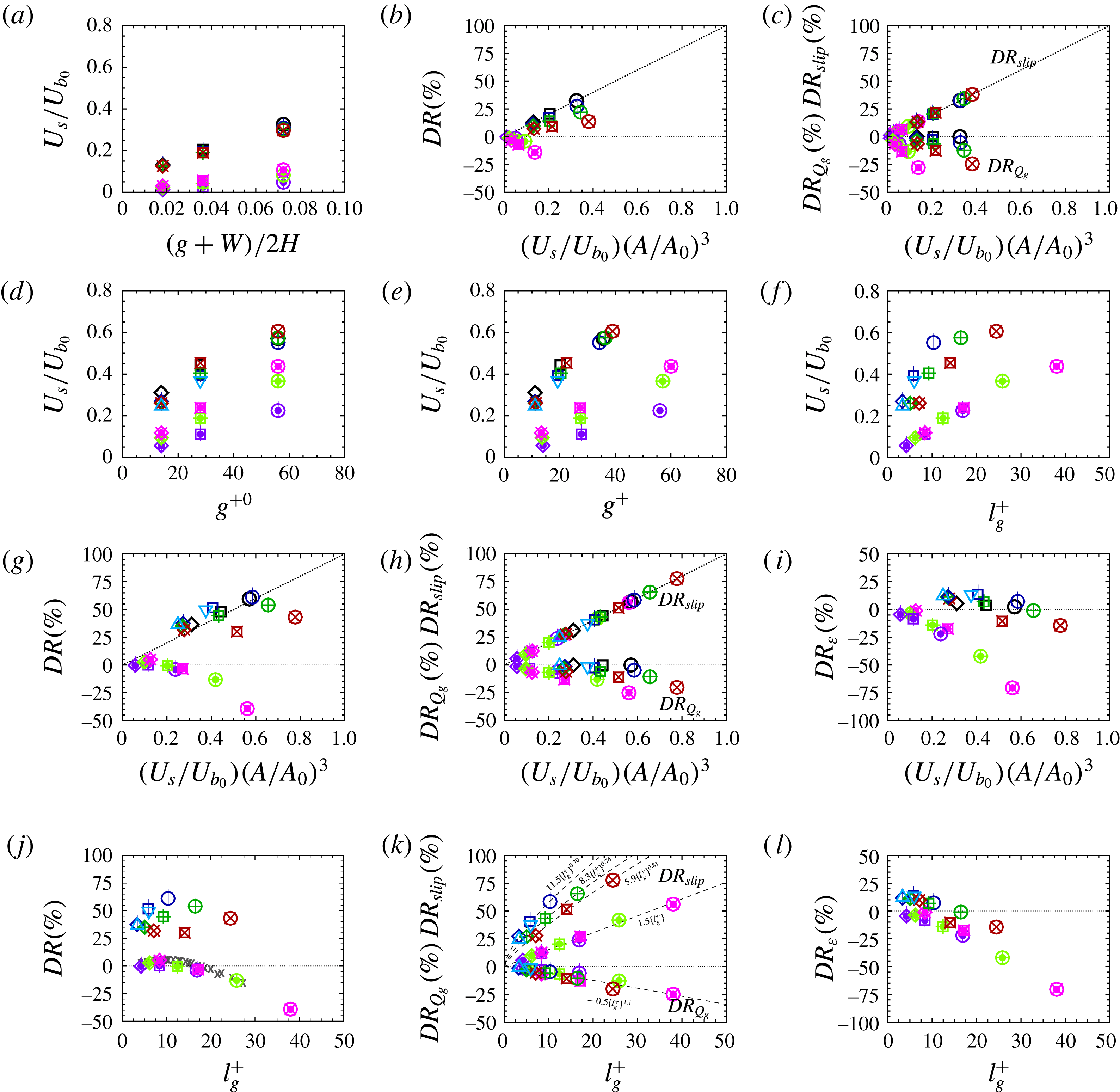
Decomposition of
 $DR_{\unicode[STIX]{x1D700}}$
into its constitutive elements: (a)
 $DR_{\langle \unicode[STIX]{x1D70F}_{R}\rangle }$
; (b)
 $DR_{\langle \unicode[STIX]{x1D70F}_{c}\rangle }$
; (c)
 $DR_{\langle \unicode[STIX]{x1D70F}_{R}\rangle _{Re_{b_{e}}}}\!$
; (d)
 $DR_{\langle \unicode[STIX]{x1D70F}_{R}\rangle _{mod}}$
. Symbols as in figure 2.
In laminar flow, (3.7) or (3.10) reduce to
 $DR=\{DR_{slip}\}+\{DR_{Q_{g}}\}$
, where
 $\{DR_{slip}\}=\{(A/A_{0})^{3}(U_{s}/U_{b_{0}})\}$
and
 $\{DR_{Q_{g}}\}=\{1-(A/A_{0})^{3}(1-Q_{g}/Q)\}$
. The wall slip velocity,
 $(U_{s}/U_{b_{0}})$
, increases with increasing microgroove width for both SH longitudinal microgrooves and riblets, as shown in figure 2(a) and table 1. However, the slip velocities obtained with SH longitudinal microgrooves are
 ${\sim}3{-}10$
times larger than those obtained with riblets, depending on the microgroove width and depth. The interface protrusion angle has a relatively minor effect on the magnitude of the slip velocity with SH longitudinal microgrooves, leading to drops of no more than 5–10 % in
 $(U_{s}/U_{b_{0}})$
with increasing protrusion angle, compared to flat interfaces. With riblets, however, the wall slip velocity increases by factors of
 ${\sim}2.2{-}2.5$
as the riblet microgroove depth increases from
 $d/g\approx 0.13$
, at
 $\unicode[STIX]{x1D703}=-30^{\circ }$
, to
 $d/g=0.5$
, at
 $\unicode[STIX]{x1D703}=-90^{\circ }$
. Both the drop in SH longitudinal microgroove slip velocity with protrusion angle and the increase in riblet slip velocity with microgroove depth reflect the displacement of the slip or no-slip boundaries away from the microgroove tips with increasing protrusion angle or microgroove depth.
The presence of an effective wall slip velocity,
 $U_{s}$
, implies that a fraction
 $(U_{s}/U_{b})=(A/A_{0})(U_{s}/U_{b_{0}})$
of the bulk velocity can flow inviscidly, leading to drag reduction through the
 $\{DR_{slip}\}$
term in (3.7) or (3.10). However, a part of this drag reduction is negated by
 $\{DR_{Q_{g}}\}$
, which is always drag enhancing, as shown in figure 2(c) and table 1. In laminar flow with SH longitudinal microgrooves, the drag enhancing contributions from
 $\{DR_{Q_{g}}\}$
lead only to deviations of the net drag reduction from the line
 $DR=\{DR_{slip}\}$
, while with riblets, the drag enhancing contributions from
 $\{DR_{Q_{g}}\}$
completely negate the drag reduction due to
 $\{DR_{slip}\}$
and lead to negative net drag reductions, as shown in figure 2(b) and table 1. This is the case even though the magnitudes of
 $\{DR_{Q_{g}}\}$
in laminar flow with riblets are comparable to, and only slightly higher than, those with SH longitudinal microgrooves for a given geometry of the wall micro-texture.
Similar features can also be observed for
 $\{DR_{slip}\}$
and
 $\{DR_{Q_{g}}\}$
in turbulent flow, as shown in figure 2(d,h) and table 1. For a given geometry of the surface micro-texture, the magnitudes of
 $\{DR_{Q_{g}}\}$
for SH longitudinal microgrooves and riblets remain comparable to each other and to their respective values in laminar flow, as shown in figure 2(h). However, the normalized slip velocities,
 $(U_{s}/U_{b_{0}})$
, in turbulent flow are significantly larger than those in laminar flow, by factors of
 ${\sim}2$
for SH longitudinal microgrooves, and by factors of
 ${\sim}4{-}5$
for riblets, respectively. The interface protrusion angle has a relatively minor effect on the slip velocity with SH longitudinal microgrooves in turbulent flow, as well, leading to drops of no more than
 $16\,\%$
or increases of no more than
 $6\,\%$
in
 $(U_{s}/U_{b_{0}})$
compared to flat interfaces, depending on whether the maximum interface depth is
 $d^{+}\lesssim 10$
or
 $d^{+}\gtrsim 10$
. In the former, the slip velocity decreases with increasing interface depth, similar to laminar flow, while in the latter, the trends are reversed, and the slip velocity is enhanced with increasing interface depth. With riblets, the slip velocity increases by factors of
 ${\sim}2$
, for all microgroove widths, as the riblet microgroove depth increases from
 $d/g\approx 0.13$
, at
 $\unicode[STIX]{x1D703}=-30^{\circ }$
, to
 $d/g=0.5$
at,
 $\unicode[STIX]{x1D703}=-90^{\circ }$
, similar to laminar flow.
Figure 2(e,f) shows the normalized slip velocities in turbulent flow plotted as a function of the microgroove width,
 $g^{+}$
, and as a function of the square root of the microgroove cross-sectional area,
 $l_{g}^{+}=\{A_{g}^{+}\}^{1/2}$
(Garcia-Mayoral & Jimenez Reference Garcia-Mayoral and Jimenez2011a
), respectively. The best collapse of the data is observed when the data are plotted as a function of
 $l_{g}^{+}$
, as shown in figure 2(f), in agreement with the observations of Garcia-Mayoral & Jimenez (Reference Garcia-Mayoral and Jimenez2011a
).
Figure 2(k) shows
 $\{DR_{slip}\}$
and
 $\{DR_{Q_{g}}\}$
in turbulent flow plotted as a function of
 $l_{g}^{+}$
. The trends in the data begin to emerge when they are plotted in this manner as a function of
 $l_{g}^{+}$
. The
 $\{DR_{Q_{g}}\}$
data for both SH longitudinal microgrooves and riblets nearly collapse and follow the scaling
 $\{DR_{Q_{g}}\}\sim -0.5\{l_{g}^{+}\}^{1.1}$
. The
 $\{DR_{slip}\}$
data for riblets collapse to the line
 $\{DR_{slip}\}\sim 1.5\{l_{g}^{+}\}$
, while the
 $\{DR_{slip}\}$
data for SH longitudinal microgrooves follow scalings which range from
 $\{DR_{slip}\}\sim 11.5\{l_{g}^{+}\}^{0.7}$
at
 $\unicode[STIX]{x1D703}=-30^{\circ }$
, to
 $\{DR_{slip}\}\sim 5.9\{l_{g}^{+}\}^{0.81}$
at
 $\unicode[STIX]{x1D703}=-90^{\circ }$
, indicating that with increasing microgroove depth, the scaling of
 $\{DR_{slip}\}$
with SH longitudinal microgrooves begins to approach that of riblets.
In turbulent flow, however, beyond the contributions from
 $\{DR_{slip}\}$
and
 $\{DR_{Q_{g}}\}$
, there is also an additional contribution to drag reduction from
 $\{DR_{\unicode[STIX]{x1D700}}\}$
, representing the drag reduction or drag increase arising from changes to the structure of turbulent Reynolds shear stresses and any mean flow shear stresses which develop due to the presence of the wall micro-texture, as shown by (3.7) and figure 2(i,l). When plotted as a function of
 $l_{g}^{+}$
, SH longitudinal microgrooves and riblets show nearly parallel trends in
 $\{DR_{\unicode[STIX]{x1D700}}\}$
, with the
 $\{DR_{\unicode[STIX]{x1D700}}\}$
data for SH longitudinal microgrooves shifted relative to the data for riblets, as shown in figure 2(l). With SH longitudinal microgrooves,
 $\{DR_{\unicode[STIX]{x1D700}}\}$
is drag reducing for microgrooves of characteristic size
 $l_{g}^{+}\lesssim 10.5$
, and drag enhancing for microgrooves of characteristic size
 $l_{g}^{+}\gtrsim 10.5$
, contributing up to
 ${\sim}14\,\%$
additional drag reduction or up to
 ${\sim}15\%$
drag increase, respectively. With riblets,
 $\{DR_{\unicode[STIX]{x1D700}}\}$
is always drag enhancing, but becomes strongly drag enhancing for riblets of characteristic size
 $l_{g}^{+}\gtrsim 10.5$
.
With SH longitudinal microgrooves, these contributions from
 $\{DR_{Q_{g}}\}$
and
 $\{DR_{\unicode[STIX]{x1D700}}\}$
lead only to deviations of the net drag reduction from the line
 $DR=\{DR_{slip}\}$
, as shown in figure 2(g). For a given width of the SH longitudinal microgrooves in base flow wall units, the highest and lowest drag reductions were always obtained at
 $\unicode[STIX]{x1D703}=-30^{\circ }$
and
 $\unicode[STIX]{x1D703}=-90^{\circ }$
, as shown in figure 2(g, j), resulting in drag reductions which differ from those with flat SH interfaces by up to
 $+3.6\,\%$
to
 $-18\,\%$
, respectively. The highest drag reductions, of
 ${\approx}61\,\%$
, were obtained with SH microgrooves of size
 $g^{+0}\approx 56,w^{+0}\approx 8$
at the protrusion angle of
 $\unicode[STIX]{x1D703}=-30^{\circ }$
. With riblets, the net drag reduction follows the line
 $DR=\{DR_{slip}\}$
only for microgrooves of characteristic size
 $l_{g}^{+}\lesssim 10.5$
, as shown in figure 2(g,j). For
 $l_{g}^{+}\gtrsim 10.5$
, the drag enhancing contributions from
 $\{DR_{\unicode[STIX]{x1D700}}\}$
and
 $\{DR_{Q_{g}}\}$
cause a decline in the magnitude of drag reduction, eventually leading to a net drag increase for
 $l_{g}^{+}\gtrsim 17$
. The highest magnitude of drag reduction obtained with riblets in the present study was
 $5\,\%$
, obtained for riblets of size
 $g^{+0}\approx 14,w^{+0}\approx 2$
at
 $\unicode[STIX]{x1D703}=-90^{\circ }$
(
 $l_{g}^{+}\sim 8.5$
). The magnitudes of drag reduction observed with riblets in the present study are consistent with experimental measurements reported by Bechert et al. (Reference Bechert, Bruse, Hage, Van Der Hoeven and Hoppe1997) for semi-circular scalloped riblets with
 $d/g=0.5$
, as shown in figure 2(j).
To gain a better understanding of the source of the differences between
 $\{DR_{\unicode[STIX]{x1D700}}\}$
with SH longitudinal microgrooves and riblets, one can decompose
 $\{DR_{\unicode[STIX]{x1D700}}\}$
into its constitutive elements, as discussed in § 3 and shown in figure 3. To begin with, the contributions from
 $\{DR_{\unicode[STIX]{x1D700}}\}$
can be decomposed into
 $\{DR_{\unicode[STIX]{x1D700}}\}=\{DR_{\langle \unicode[STIX]{x1D70F}_{R}\rangle }\}+\{DR_{\langle \unicode[STIX]{x1D70F}_{c}\rangle }\}$
, as shown by (3.10), where
 $\{DR_{\langle \unicode[STIX]{x1D70F}_{R}\rangle }\}$
and
 $\{DR_{\langle \unicode[STIX]{x1D70F}_{c}\rangle }\}$
represent the contributions to drag reduction arising from modifications to the normalized structure of turbulent Reynolds shear stresses and any mean flow shear stresses which develop due to the presence of the wall micro-texture, respectively. DNS results, displayed in figure 3(a,b), show that
 $\{DR_{\langle \unicode[STIX]{x1D70F}_{R}\rangle }\}$
is drag reducing for SH longitudinal microgrooves of depth
 $d^{+}\lesssim 10.5$
, but drag enhancing with riblets of any size and SH longitudinal microgrooves of depth
 $d^{+}\gtrsim 10.5$
, while
 $\{DR_{\langle \unicode[STIX]{x1D70F}_{c}\rangle }\}$
is always drag enhancing and follows a common scaling with both SH longitudinal microgrooves and riblets when plotted as a function of
 $l_{g}^{+}$
. The finding that
 $DR_{\langle \unicode[STIX]{x1D70F}_{R}\rangle }$
is always drag enhancing with riblets stands in contrast with current understanding of the mechanism of drag reduction with riblets, which attributes at least part of the drag reduction with riblets to the weakening of turbulent vortical structures (Bechert & Bartenwerfer Reference Bechert and Bartenwerfer1989; Walsh Reference Walsh, Bushnell and Hefner1990; Luchini et al.
Reference Luchini, Manzo and Pozzi1991; Chu & Karniadakis Reference Chu and Karniadakis1993; Goldstein et al.
Reference Goldstein, Handler and Sirovich1995; Bechert et al.
Reference Bechert, Bruse, Hage, Van Der Hoeven and Hoppe1997; Garcia-Mayoral & Jimenez Reference Garcia-Mayoral and Jimenez2011a
).
The differences between
 $\{DR_{\langle \unicode[STIX]{x1D70F}_{R}\rangle }\}$
with SH longitudinal microgrooves and riblets can be further understood by decomposing
 $\{DR_{\langle \unicode[STIX]{x1D70F}_{R}\rangle }\}$
into
 $\{DR_{\langle \unicode[STIX]{x1D70F}_{R}\rangle }\}=\{DR_{\langle \unicode[STIX]{x1D70F}_{R}\rangle _{Re_{b_{e}}}}\}+\{DR_{\langle \unicode[STIX]{x1D70F}_{R}\rangle _{mod}}\}$
, as shown in (3.10) and figure 3(c,d), where
 $\{DR_{\langle \unicode[STIX]{x1D70F}_{R}\rangle _{Re_{b_{e}}}}\}$
represents the contributions to drag reduction arising from changes to the normalized structure of turbulent Reynolds shear stresses due to the presence of an effective slip velocity,
 $U_{s}$
, at the wall, which in effect reduces the bulk Reynolds number of the viscous part of the flow from
 $Re_{b}$
to
 $Re_{b_{e}}=(1-U_{s}/U_{b})Re_{b}$
, while
 $\{DR_{\langle \unicode[STIX]{x1D70F}_{R}\rangle _{mod}}\}$
represents the contributions to drag reduction arising from any other modifications to the normalized structure of turbulent Reynolds shear stresses in the presence of the surface micro-texture. By definition, the contributions from
 $\{DR_{\langle \unicode[STIX]{x1D70F}_{R}\rangle _{Re_{b_{e}}}}\}$
are always drag reducing. Figure 3(c,d) shows that these contributions follow nearly parallel trends with SH longitudinal microgrooves and riblets, while the contributions from
 $\{DR_{\langle \unicode[STIX]{x1D70F}_{R}\rangle _{mod}}\}$
are always drag enhancing and follow a common scaling with SH longitudinal microgrooves and riblets when plotted as a function of
 $l_{g}^{+}$
.
The results displayed in figures 2 and 3 quantify and clarify the contribution of each of the five terms in (3.10) to the net drag reduction with SH longitudinal microgrooves or riblets in laminar or turbulent flow. These five contributions are: (i) the effective slip velocity at the wall, which allows a fraction
 $(U_{s}/U_{b})$
of the flow rate to be carried inviscidly, represented by
 $\{DR_{slip}\}$
; (ii) modifications to the normalized structure of turbulent Reynolds shear stresses due to the drop in the bulk Reynolds number of the ‘viscous’ part of the flow, from
 $Re_{b}$
to
 $Re_{b_{e}}=(1-U_{s}/U_{b})Re_{b}$
, because of the presence of this effective slip velocity at the wall, represented by
 $\{DR_{\langle \unicode[STIX]{x1D70F}_{R}\rangle _{Re_{b_{e}}}}\}$
; (iii) other modifications to the normalized structure of turbulent Reynolds shear stresses due to the presence of the surface micro-texture, represented by
 $\{DR_{\langle \unicode[STIX]{x1D70F}_{R}\rangle _{mod}}\}$
; (iv) mean flow shear stresses developed due to presence of the surface micro-texture, represented by
 $\{DR_{\langle \unicode[STIX]{x1D70F}_{c}\rangle }\}$
; and (v) the fraction of the flow rate through the surface micro-texture, represented by
 $\{DR_{Q_{g}}\}$
.
DNS results with SH longitudinal microgrooves and riblets, displayed in figures 2(c,k) and 3(b–d), show that SH longitudinal microgrooves and riblets share a common mechanism of drag reduction, in which 100 % of the drag reduction arises from effects (i) and (ii). The contributions from (iii)–(v) were always drag enhancing, and followed common scalings with SH longitudinal microgrooves and riblets when expressed as a function of
 $l_{g}^{+}$
. These results indicate that the differences in the drag reduction performance of SH longitudinal microgrooves and riblets can be attributed entirely to the different magnitudes of the effective slip velocity which can be achieved in the two flows.
4.2 Turbulence statistics
The common mechanism of drag reduction with SH longitudinal microgrooves and riblets also leads to common features in the normalized profiles of the spanwise-averaged mean streamwise velocities,
 $\langle \overline{U}\rangle ^{+}$
, turbulence intensities,
 $\{\langle \overline{u_{i}^{2}}\rangle ^{1/2}\}^{+}$
, Reynolds shear stresses,
 $\langle \unicode[STIX]{x1D70F}_{R,xz}\rangle ^{+}$
, and mean convective shear stresses,
 $\langle \unicode[STIX]{x1D70F}_{c,xz}\rangle ^{+}$
, in the two flows, as shown in figure 4. With the effective wall slip velocity subtracted, the mean streamwise velocity profiles,
 $\langle \overline{U}\rangle ^{+}-U_{s}^{+}$
, with both SH longitudinal microgrooves and riblets display a shortening of the viscous sublayer and the buffer layer, and a downward shift of the logarithmic layer, with comparable magnitudes of the shift for SH longitudinal microgrooves and riblets of comparable characteristic size,
 $l_{g}^{+}$
, as shown in figures 4(a,d), 4(g,j) and 4(m,p). These features provide further confirmation of the findings in § 4.1 that, beyond the effect of
 $U_{s}$
, the presence of the wall micro-texture leads only to drag enhancement through the
 $\{DR_{\langle \unicode[STIX]{x1D70F}_{R}\rangle _{mod}}\}$
and
 $\{DR_{\langle \unicode[STIX]{x1D70F}_{c}\rangle }\}$
terms, and that these two terms have similar effects on the structure and dynamics of turbulence with SH longitudinal microgrooves and riblets of a given characteristic size,
 $l_{g}^{+}$
.
Turbulence statistics in channel flow with (a–c, g–i, m–o) SH longitudinal microgrooves (LMGs), and (d–f, j–l, p–r) riblets, compared to channel flow with smooth, no-slip walls: (a,d,g,j,m,p) mean streamwise velocity with the effective wall slip velocity subtracted; (b,e,h,k,n,q) turbulence intensities; (c,f,i,l,o,r) Reynolds shear stress,
 $\langle \unicode[STIX]{x1D70F}_{R,xz}\rangle ^{+}=-\unicode[STIX]{x1D70C}\langle \overline{uw}\rangle ^{+}$
, viscous shear stress,
 $\langle \unicode[STIX]{x1D70F}_{v,xz}\rangle ^{+}=\langle \unicode[STIX]{x1D707}\unicode[STIX]{x2202}\bar{U}/\unicode[STIX]{x2202}z\rangle ^{+}$
, mean convective stress,
 $\langle \unicode[STIX]{x1D70F}_{c,xz}\rangle ^{+}=-\unicode[STIX]{x1D70C}\langle \bar{U}\bar{W}\rangle ^{+}$
, and total shear stress,
 $\langle \unicode[STIX]{x1D70F}_{t}\rangle ^{+}=\langle \unicode[STIX]{x1D70F}_{R,xz}\rangle ^{+}+\langle \unicode[STIX]{x1D70F}_{v,xz}\rangle ^{+}+\langle \unicode[STIX]{x1D70F}_{c,xz}\rangle ^{+}$
.

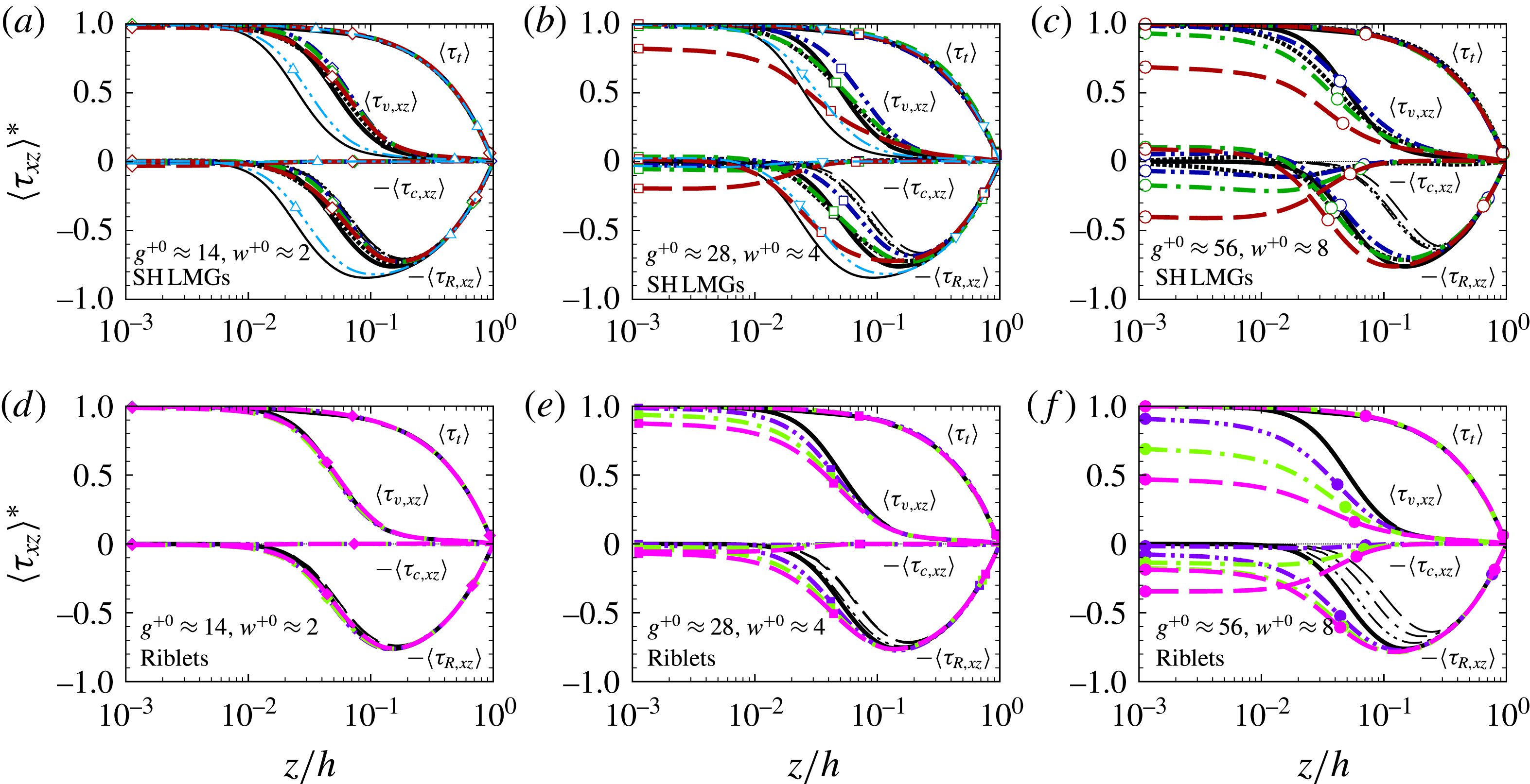
Shear stresses,
 $\langle \unicode[STIX]{x1D70F}\rangle ^{\ast }=\langle \unicode[STIX]{x1D70F}\rangle /(-\langle \unicode[STIX]{x2202}\bar{P}/\unicode[STIX]{x2202}x\rangle h)=(A/A_{0})\langle \unicode[STIX]{x1D70F}\rangle ^{+}$
, in turbulent channel flow with (a–c) SH longitudinal microgrooves, and (d–f) riblets, compared to turbulent channel flow with smooth, no-slip walls.
 $\cdots \cdots$
, — ⋅ ⋅ —, — ⋅ —, – – –, Reynolds shear stress,
 $\langle \unicode[STIX]{x1D70F}_{R,xz}\rangle _{Re_{b_{e}}}^{\ast }$
, in a smooth, no-slip turbulent channel flow at bulk Reynolds number equal to
 $Re_{b_{e}}$
of the corresponding SH or riblet case with
 $\unicode[STIX]{x1D703}=0^{\circ }$
,
 $\unicode[STIX]{x1D703}=-30^{\circ }$
,
 $\unicode[STIX]{x1D703}=-60^{\circ }$
and
 $\unicode[STIX]{x1D703}=-90^{\circ }$
and
 $Re_{b}=3600$
, respectively. Other line types as in figure 4.
The normalized profiles of turbulence intensities with both SH longitudinal microgrooves and riblets show enhanced magnitudes of turbulence intensities, compared to the base flow, within a ‘surface layer’ of thickness
 ${\sim}2g$
, for all components of turbulent velocity fluctuations, as shown in figures 4(b,e), 4(h,k) and 4(n,q). These enhanced turbulence intensities result from additional production of streamwise turbulence kinetic energy, due to presence of spanwise gradients of the Reynolds-averaged streamwise velocity,
 $\unicode[STIX]{x2202}\overline{U}/\unicode[STIX]{x2202}y$
, between the slip and no-slip regions at the tip of the surface micro-texture, which are then transferred to the wall-normal and cross-stream components of the turbulent velocity fluctuations through the pressure-strain terms.
The changes to the structure of turbulence and the mean flow affect the drag reduction only through the changes in the Reynolds shear stresses,
 $\langle \unicode[STIX]{x1D70F}_{R,xz}\rangle$
, and mean convective shear stresses,
 $\langle \unicode[STIX]{x1D70F}_{c,xz}\rangle$
, compared to the base flow, as shown by the
 $\{DR_{\langle \unicode[STIX]{x1D70F}_{R}\rangle }\}$
and
 $\{DR_{\langle \unicode[STIX]{x1D70F}_{c}\rangle }\}$
terms in (3.10). These shear stresses are displayed in figure 4(c,f,i,l,o,r) and figure 5(a–f). In the latter, the stresses are shown in the normalization,
 $\langle \unicode[STIX]{x1D70F}\rangle ^{\ast }=\langle \unicode[STIX]{x1D70F}\rangle /(-\langle \unicode[STIX]{x2202}\bar{P}/\unicode[STIX]{x2202}x\rangle h)=(A/A_{0})\langle \unicode[STIX]{x1D70F}\rangle ^{+}$
, which appears in (3.10).
The presence of the surface micro-texture gives rise to non-zero mean convective shear stresses,
 $\langle \unicode[STIX]{x1D70F}_{c,xz}\rangle$
, in turbulent flow within the ‘surface layer’, as discussed in Rastegari & Akhavan (Reference Rastegari and Akhavan2015). These mean flow shear stresses have a common structure for SH longitudinal microgrooves and riblets of a given characteristic size,
 $l_{g}^{+}$
, and always have a drag enhancing contribution to drag reduction, as shown in figures 4(c,f,i,l,o,r), 5(a,d,b,e,c,f) and 3(b).
The presence of the surface micro-texture also gives rise to changes in the structure of normalized Reynolds shear stresses,
 $\langle \unicode[STIX]{x1D70F}_{R,xz}\rangle ^{\ast }$
, compared to the base flow, as shown in figure 5. These changes contribute to drag reduction through the
 $\{DR_{\langle \unicode[STIX]{x1D70F}_{R}\rangle }\}$
term in (3.10), and can be either drag reducing or drag enhancing, as shown in figure 3(a). Unlike other examples of drag-reduced turbulent flow, where drag reduction is accompanied by dramatic changes to the normalized Reynolds shear stresses, the changes to
 $\langle \unicode[STIX]{x1D70F}_{R,xz}\rangle ^{\ast }$
in drag reduction with micro-textured surfaces are subtle, and confined to a thin ‘surface layer’ of thickness
 ${\sim}2g$
, once again confirming that the main mechanism of drag reduction with micro-textured surfaces is surface slip. Figure 5(a–c) shows that for all SH longitudinal microgrooves with a microgroove depth
 $d^{+}\lesssim 10.5$
, the normalized Reynolds shear stresses,
 $\langle \unicode[STIX]{x1D70F}_{R,xz}\rangle ^{\ast }$
, have a lower magnitude within the surface layer compared to the base flow, giving rise to drag reducing contributions from
 $\{DR_{\langle \unicode[STIX]{x1D70F}_{R}\rangle }\}$
, as observed for these cases in figure 3(a). The only SH cases for which
 $\langle \unicode[STIX]{x1D70F}_{R,xz}\rangle ^{\ast }$
had a higher magnitude within the surface layer compared to the base flow were the SH microgrooves with
 $g^{+0}\approx 28$
and
 $g^{+0}\approx 56$
at
 $\unicode[STIX]{x1D703}=-90^{\circ }$
, for which
 $d^{+}\gtrsim 10.5$
, and
 $\{DR_{\langle \unicode[STIX]{x1D70F}_{R}\rangle }\}$
is, accordingly, drag enhancing. With riblets, on the other hand,
 $\langle \unicode[STIX]{x1D70F}_{R,xz}\rangle ^{\ast }$
always had a higher magnitude within the surface layer compared to the base flow, as shown in figure 5(d–f), giving rise to drag enhancing contributions from
 $\{DR_{\langle \unicode[STIX]{x1D70F}_{R}\rangle }\}$
, as observed for riblets in figure 3(a).
Figure 5(a–f) also shows the Reynolds shear stresses,
 $\langle \unicode[STIX]{x1D70F}_{R,xz}\rangle _{Re_{b_{e}}}^{\ast }$
, which would be obtained in a smooth, no-slip channel flow at a bulk Reynolds number equal to
 $Re_{b_{e}}$
of the corresponding SH longitudinal microgroove or riblet case. The differences between these
 $\langle \unicode[STIX]{x1D70F}_{R,xz}\rangle _{Re_{b_{e}}}^{\ast }$
and
 $\langle \unicode[STIX]{x1D70F}_{R,xz}\rangle _{0}^{\ast }$
in the base flow represent the effect of the wall slip velocity,
 $U_{s}$
, on the turbulent Reynolds shear stresses, and give rise to the drag reducing contributions from
 $\{DR_{\langle \unicode[STIX]{x1D70F}_{R}\rangle _{Re_{b_{e}}}}\}$
observed in figure 3(c). Similarly, the differences between
 $\langle \unicode[STIX]{x1D70F}_{R,xz}\rangle ^{\ast }$
in the flows with micro-textured walls and these
 $\langle \unicode[STIX]{x1D70F}_{R,xz}\rangle _{Re_{b_{e}}}^{\ast }$
represent other modifications to the normalized structure of turbulent shear stresses due to the presence of the surface micro-texture, beyond the effect of
 $U_{s}$
, and give rise to the drag enhancing contributions from
 $\{DR_{\langle \unicode[STIX]{x1D70F}_{R}\rangle _{mod}}\}$
observed in figure 3(d). In general, the presence of surface micro-texture has two competing effects on the normalized structure and dynamics of Reynolds shear stresses and near-wall vortical structures: a weakening effect due to establishment of streamwise surface slip, and a strengthening effect due to establishment of spanwise surface slip. The streamwise slip gives rise to the differences between
 $\langle \unicode[STIX]{x1D70F}_{R,xz}\rangle _{Re_{b_{e}}}^{\ast }$
and
 $\langle \unicode[STIX]{x1D70F}_{R,xz}\rangle _{0}^{\ast }$
in the base flow, while the spanwise slip gives rise to the differences between
 $\langle \unicode[STIX]{x1D70F}_{R,xz}\rangle ^{\ast }$
in the flows with micro-textured walls and
 $\langle \unicode[STIX]{x1D70F}_{R,xz}\rangle _{Re_{b_{e}}}^{\ast }$
.
Root-mean-square (r.m.s.) streamwise vorticity fluctuations in turbulent channel flow with (a–c) SH longitudinal microgrooves, and (d–f) riblets, compared to base channel flow with smooth, no-slip walls.
 $\cdots \cdots$
, — ⋅ ⋅ —, — ⋅ —, – – –, streamwise r.m.s. vorticity fluctuations,
 $\{\langle \overline{\unicode[STIX]{x1D714}_{x}^{2}}\rangle ^{1/2}\}_{Re_{b_{e}}}^{+}$
, in a smooth, no-slip turbulent channel flow at bulk Reynolds number equal to
 $Re_{b_{e}}$
of the corresponding SH or riblet case with
 $\unicode[STIX]{x1D703}=0^{\circ }$
,
 $\unicode[STIX]{x1D703}=-30^{\circ }$
,
 $\unicode[STIX]{x1D703}=-60^{\circ }$
and
 $\unicode[STIX]{x1D703}=-90^{\circ }$
and
 $Re_{b}=3600$
, respectively. Other line types as in figure 4.
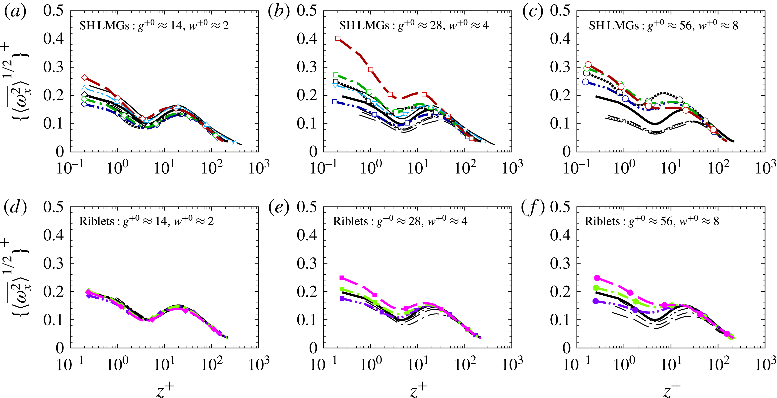
Similar features can also be observed with the near-wall streamwise vortical structures, as shown in figure 6. The presence of streamwise surface slip results in a weakening of the streamwise vorticity fluctuations within the ‘surface layer’ to the magnitudes shown for
 $\{\langle \overline{\unicode[STIX]{x1D714}_{x}^{2}}\rangle ^{1/2}\}_{Re_{b_{e}}}^{+}$
in each figure, while the presence of spanwise surface slip strengthens the near-wall streamwise vorticity fluctuations from their
 $\{\langle \overline{\unicode[STIX]{x1D714}_{x}^{2}}\rangle ^{1/2}\}_{Re_{b_{e}}}^{+}$
values back to magnitudes which can be either smaller or greater than those in the base flow. In general, for SH longitudinal microgrooves of characteristic size
 $l_{g}^{+}\lesssim 7$
and riblets of characteristic size
 $l_{g}^{+}\lesssim 8.5$
, the magnitudes of
 $\{\langle \overline{\unicode[STIX]{x1D714}_{x}^{2}}\rangle ^{1/2}\}^{+}$
within the ‘surface layer’ fell below those in the base flow. For a given width,
 $g^{+0}$
, of the microgrooves in base flow wall units, the lowest and highest magnitudes of
 $\{\langle \overline{\unicode[STIX]{x1D714}_{x}^{2}}\rangle ^{1/2}\}^{+}$
were always observed at
 $\unicode[STIX]{x1D703}=-30^{\circ }$
and
 $\unicode[STIX]{x1D703}=-90^{\circ }$
, respectively, with both SH longitudinal microgrooves and riblets.
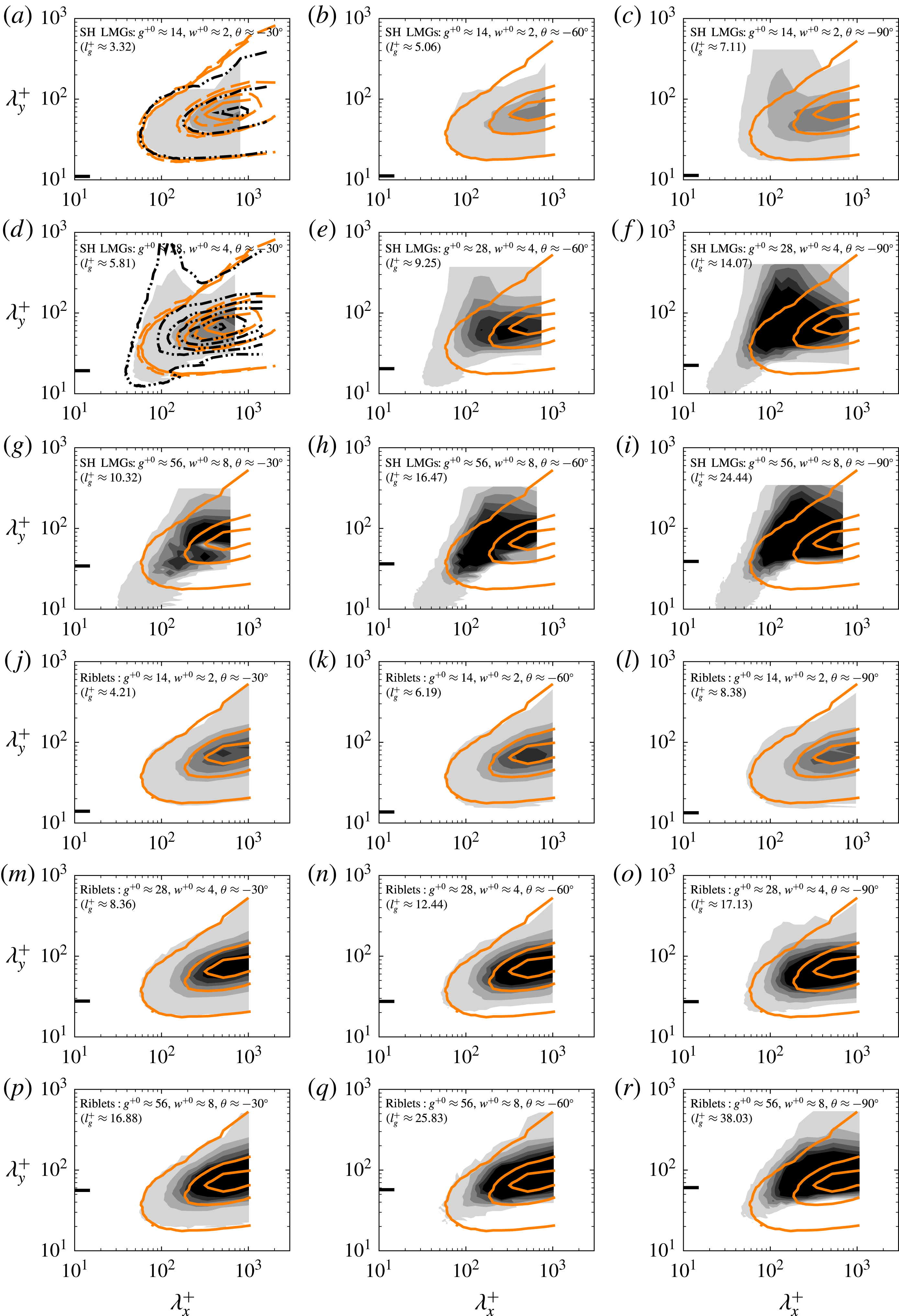
Pre-multiplied two-dimensional co-spectra of the Reynolds shear stress,
 $k_{x}^{+}k_{y}^{+}E_{uw}^{+}$
, at
 $z^{+}\approx 5$
, in turbulent channel flow with (a–i) SH longitudinal microgrooves, and (j–r) riblets, compared to turbulent channel flow with smooth, no-slip walls. Shaded contours correspond to channels with SH longitudinal microgrooves or riblets at
 $Re_{b}=3600$
; — ⋅ ⋅ — (black), contour lines in channels with SH longitudinal microgrooves at
 $Re_{b}=7860$
; ——, – – – (orange), contour lines in channels with smooth, no-slip walls at
 $Re_{b}=3600$
and
 $Re_{b}=7860$
, respectively. Contour levels at
 $(0.00025:0.01:0.05025)$
. The tick mark on the left of each plot marks the microgroove width.
4.3 Role of spanwise rollers
It has been suggested that the drag enhancing features observed in
 $\{DR_{\unicode[STIX]{x1D700}}\}$
and
 $\{DR_{\langle \unicode[STIX]{x1D70F}_{R}\rangle }\}$
with riblets are caused by the appearance of long spanwise rollers in the region below
 $z^{+}\approx 15{-}20$
, with typical streamwise wavelengths of
 $\unicode[STIX]{x1D706}_{x}^{+}\approx 150$
, that develop from a two-dimensional Kelvin–Helmholtz–like instability of the mean streamwise flow (Garcia-Mayoral & Jimenez Reference Garcia-Mayoral and Jimenez2011a
,Reference Garcia-Mayoral and Jimenez
b
, Reference Garcia-Mayoral and Jimenez2012). These rollers can be visualized by examining the pre-multiplied, two-dimensional co-spectra of the Reynolds shear stress at a location below
 $z^{+}\approx 15-20$
. Figure 7 shows these co-spectra at
 $z^{+}\approx 5$
for all the SH longitudinal microgroove and riblet cases investigated in the present study. The presence of spanwise rollers is manifested by accumulation of spectral energy near
 $\unicode[STIX]{x1D706}_{x}^{+}\approx 150$
for spanwise wavelengths longer than
 $\unicode[STIX]{x1D706}_{y}^{+}\approx 100$
, representing elongated structures in the spanwise direction. The strongest evidence of the presence of these spanwise rollers can be seen with SH longitudinal microgrooves in figure 7(c–i). However, with the exception of the two cases represented by figure 7(f,i), all other SH cases have a drag reducing contribution from both
 $\{DR_{\unicode[STIX]{x1D700}}\}$
and
 $\{DR_{\langle \unicode[STIX]{x1D70F}_{R}\rangle }\}$
. Similarly, with riblets, where there is a drag enhancing contribution from
 $\{DR_{\unicode[STIX]{x1D700}}\}$
and
 $\{DR_{\langle \unicode[STIX]{x1D70F}_{R}\rangle }\}$
for all cases, the evidence of the presence of rollers is fairly weak, and can only be seen in figure 7(o,r).
These results indicate that there is no correlation between the appearance of spanwise rollers and whether the contributions from
 $\{DR_{\unicode[STIX]{x1D700}}\}$
and
 $\{DR_{\langle \unicode[STIX]{x1D70F}_{R}\rangle }\}$
are drag reducing or drag enhancing. Instead, the appearance of the spanwise rollers seems to be correlated with the depth of the microgrooves and presence of an effective wall slip velocity
 $U_{s}^{+}\gtrsim 5{-}6$
, with both SH longitudinal microgrooves and riblets.
5 Extrapolation of DNS results to high Reynolds number flows of practical interest
To explore the effect of bulk Reynolds number of the flow on the dynamics reported in § 4, two of the SH simulations, corresponding to longitudinal microgrooves of size
 $g^{+0}\approx 14$
and
 $g^{+0}\approx 28$
with
 $\unicode[STIX]{x1D703}=-30^{\circ }$
, were repeated at
 $Re_{b}=7860$
. These simulations correspond to a doubling of the friction Reynolds number of the base flow from
 $Re_{\unicode[STIX]{x1D70F}_{0}}\approx 222$
at
 $Re_{b}=3600$
, to
 $Re_{\unicode[STIX]{x1D70F}_{0}}\approx 442$
at
 $Re_{b}=7860$
. The results of these higher Reynolds number simulations are also shown in table 1 and figures 2–7. The differences between the results at
 $Re_{b}=3600$
and
 $Re_{b}=7860$
are slight, confirming that the lower Reynolds number simulations properly capture the essential features of drag reduction with micro-textured surfaces in turbulent flows at higher Reynolds numbers.
By increasing the Reynolds number of the flow from
 $Re_{b}=3600$
to
 $Re_{b}=7860$
, the magnitudes of drag reduction with SH longitudinal microgrooves of size
 $g^{+0}\approx 14$
and
 $g^{+0}\approx 28$
with
 $\unicode[STIX]{x1D703}=-30^{\circ }$
dropped to
 ${\approx}98\,\%$
and
 ${\approx}96\,\%$
of their respective values at
 $Re_{b}=3600$
, as shown in table 1. In general, as originally demonstrated by Bechert et al. (Reference Bechert, Bruse, Hage, Van Der Hoeven and Hoppe1997) and Spalart & McLean (Reference Spalart and Mclean2011), and discussed in more detail in this section, the drag reduction performance of micro-textured surfaces, with a given geometry and size of the wall micro-texture in wall units, degrades with increasing bulk Reynolds number of the flow, due to the drop in the friction coefficient,
 $C_{f_{0}}$
, of the base flow with increasing bulk Reynolds number. The main source of this degradation in drag reduction performance is a drop in the magnitude of
 $\{DR_{slip}\}$
with increasing bulk Reynolds number. The reason for this drop can be understood by noting that the slip velocity normalized in wall units,
 $U_{s}^{+}$
, remains invariant with the Reynolds number for a given characteristic size of the microgrooves,
 $l_{g}^{+}$
, as shown in table 1. Consequently, quantities which are proportional to
 $(U_{s}/U_{b})$
, such as
 $\{DR_{slip}\}$
, will experience a degradation with increasing Reynolds number, approximately proportional to the ratios of
 $\sqrt{C_{f_{0}}}$
in their respective base flows. In the present study, this effect results in
 $\{DR_{slip}\}$
values at
 $Re_{b}=7860$
which are 91–92 % of the values as
 $Re_{b}=3600$
, which is approximately equal to the ratio of
 $\sqrt{C_{f_{0}}}$
in the ‘base’ flows at
 $Re_{b}=7860$
and
 $Re_{b}=3600$
. Part of this drop in drag reduction due to
 $\{DR_{slip}\}$
is compensated by
 $\{DR_{Q_{g}}\}$
, which becomes less drag enhancing with increasing bulk Reynolds number of the base flow. In general,
 $\{DR_{Q_{g}}\}$
represents a low Reynolds number effect and its magnitude should become negligible at high Reynolds numbers. The percentage of drag reduction arising from
 $\{DR_{\unicode[STIX]{x1D700}}\}$
remained approximately unchanged for the two Reynolds numbers investigated in the present study.
Aside from these adjustments to the magnitude of
 $DR$
, the other features of drag-reduced flows at
 $Re_{b}=7860$
, including the characteristics of mean velocity profiles, turbulence intensities, Reynolds shear stresses, mean flow shear stresses, streamwise vorticity fluctuations, and two-dimensional co-spectra remained similar to those described for
 $Re_{b}=3600$
, as shown in figures 4–7. These findings are consistent with observations by a number of other investigators (Garcia-Mayoral & Jimenez Reference Garcia-Mayoral and Jimenez2012; Park et al.
Reference Park, Park and Kim2013; Seo et al.
Reference Seo, Garcia-Mayoral and Mani2015), who have also found little effect of Reynolds number on the physics of drag reduction with micro-textured surfaces, and have concluded that the physics deduced from DNS studies at
 $Re_{\unicode[STIX]{x1D70F}_{0}}\approx 200$
contain the essential features of drag reduction found in higher Reynolds number turbulent flows.
Streamwise mean velocity profiles in turbulent channel flow with micro-textured walls compared to turbulent channel flow with smooth, no-slip walls: (a) general characteristics of the mean velocity profiles in the presence of micro-textured walls; (b–d) mean velocity profiles in turbulent channel flow with SH longitudinal microgrooves or riblets. Line types in (b–d) as in figure 4.
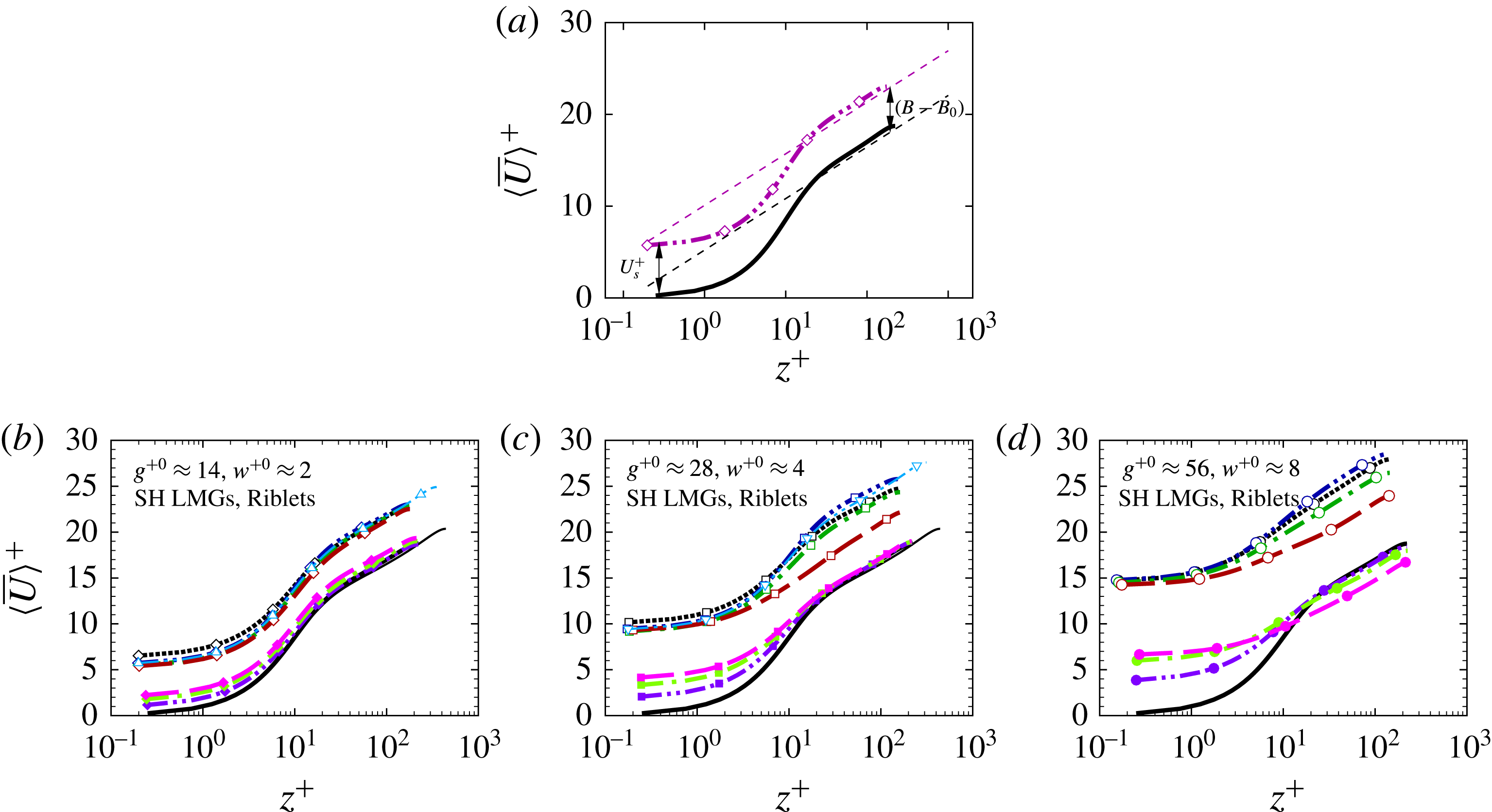
The drag reduction results obtained in DNS can be extended to higher Reynolds number flows of practical interest, using the parameterization of
 $DR$
in terms of the shift in the intercept of a logarithmic-law representation of the mean velocity profiles, as suggested by Bechert et al. (Reference Bechert, Bruse, Hage, Van Der Hoeven and Hoppe1997) and Spalart & McLean (Reference Spalart and Mclean2011). In this parameterization, the mean velocity profiles in the channel flows with micro-textured walls and in the base channel flow with smooth, no-slip walls are each approximated by logarithmic velocity profiles throughout the cross-section of the channel, as shown in figure 8. These logarithmic profiles are then integrated, and set equal to the bulk velocity, to get
 $$\begin{eqnarray}\displaystyle & \displaystyle \frac{U_{b}}{u_{\unicode[STIX]{x1D70F}}}=\frac{1}{h}\int _{0}^{h}\left(\frac{1}{\unicode[STIX]{x1D705}}\ln z^{+}+B\right)\,\text{d}z=\frac{1}{\unicode[STIX]{x1D705}}\ln \left(Re_{b}\sqrt{\frac{C_{f}}{2}}\right)+\left(B-\frac{1}{\unicode[STIX]{x1D705}}\right), & \displaystyle\end{eqnarray}$$
 $$\begin{eqnarray}\displaystyle & \displaystyle \frac{U_{b_{0}}}{u_{\unicode[STIX]{x1D70F}_{0}}}=\frac{1}{h}\int _{0}^{h}\left(\frac{1}{\unicode[STIX]{x1D705}}\ln z^{+}+B_{0}\right)\,\text{d}z=\frac{1}{\unicode[STIX]{x1D705}}\ln \left(Re_{b}\sqrt{\frac{C_{f_{0}}}{2}}\right)+\left(B_{0}-\frac{1}{\unicode[STIX]{x1D705}}\right), & \displaystyle\end{eqnarray}$$
where
 $\unicode[STIX]{x1D705}$
is the von Kármán constant, and
 $B$
and
 $B_{0}$
are the intercepts of logarithmic-law representations of the mean velocity profiles in the channel flow with micro-textured walls and the channel flow with smooth, no-slip walls, respectively, as shown in figure 8(a).
Using the definitions
 $U_{b}/u_{\unicode[STIX]{x1D70F}}=\sqrt{2/C_{f}}$
and
 $U_{b_{0}}/u_{\unicode[STIX]{x1D70F}_{0}}=\sqrt{2/C_{f_{0}}}$
, (5.1) and (5.2) can be combined to give an expression for
 $DR=(1-C_{f}/C_{f_{0}})$
as
 $$\begin{eqnarray}(1-DR)=\left\{1+\left[\frac{1}{2\unicode[STIX]{x1D705}}\ln (1-DR)+(B-B_{0})\right]\sqrt{\frac{C_{f_{0}}}{2}}\right\}^{-2}.\end{eqnarray}$$
Equation (5.3) provides a parameterization of
 $DR$
in terms of the shift,
 $(B-B_{0})$
, of a logarithmic-law representation of the mean velocity profile in the flow with micro-textured walls compared to the base flow. Approximate forms of (5.3), for the limit of low drag reduction, have been earlier derived for riblets (Bechert et al.
Reference Bechert, Bruse, Hage, Van Der Hoeven and Hoppe1997; Spalart & McLean Reference Spalart and Mclean2011). In this limit, (5.3) can be approximated by
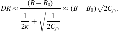 $$\begin{eqnarray}DR\approx \frac{(B-B_{0})}{\displaystyle \frac{1}{2\unicode[STIX]{x1D705}}+\sqrt{\frac{1}{2C_{f_{0}}}}}\approx (B-B_{0})\sqrt{2C_{f_{0}}}.\end{eqnarray}$$
It has been suggested that, in drag reduction with micro-textured surfaces,
 $(B-B_{0})$
is independent of Reynolds number, and only a function of the geometrical parameters of the surface micro-texture in wall units (Clauser Reference Clauser1956; Bechert et al.
Reference Bechert, Bruse, Hage, Van Der Hoeven and Hoppe1997; Spalart & McLean Reference Spalart and Mclean2011; Garcia-Mayoral & Jimenez Reference Garcia-Mayoral and Jimenez2012). As such, (5.3) can be used to investigate the effect of the bulk Reynolds number of the flow on drag reduction with micro-textured surfaces.
Parameterization of
 $DR$
in turbulent channel flow with SH longitudinal microgrooves or riblets in terms of the shift,
 $(B-B_{0})$
, of a logarithmic-law representation of the mean velocity profile and the Reynolds number of the base flow: (a)
 $DR$
as a function of
 $(B-B_{0})$
and the friction Reynolds number of the base flow; (b)
 $(B-B_{0})$
as a function of
 $l_{g}^{+}$
; (c) average streamwise slip velocity,
 $U_{s}^{+}$
, as a function of
 $l_{g}^{+}$
; (d)
 $\{(B-B_{0})-U_{s}^{+}\}$
as a function of
 $l_{g}^{+}$
. Line types in (a): ——,
 $Re_{b}=3600$
(
 $Re_{\unicode[STIX]{x1D70F}_{0}}\approx 222$
); — —,
 $Re_{b}=7860$
(
 $Re_{\unicode[STIX]{x1D70F}_{0}}\approx 442$
); – – –,
 $Re_{b}=2\times 10^{4}$
(
 $Re_{\unicode[STIX]{x1D70F}_{0}}\approx 10^{3}$
); — ⋅ —,
 $Re_{b}=2.7\times 10^{5}$
(
 $Re_{\unicode[STIX]{x1D70F}_{0}}\approx 10^{4}$
); — ⋅ ⋅ —,
 $Re_{b}=3.8\times 10^{6}$
(
 $Re_{\unicode[STIX]{x1D70F}_{0}}\approx 10^{5}$
);
 $\cdots \cdots$
,
 $Re_{b}=5.3\times 10^{7}$
(
 $Re_{\unicode[STIX]{x1D70F}_{0}}\approx 10^{6}$
). Symbols as in figure 3.
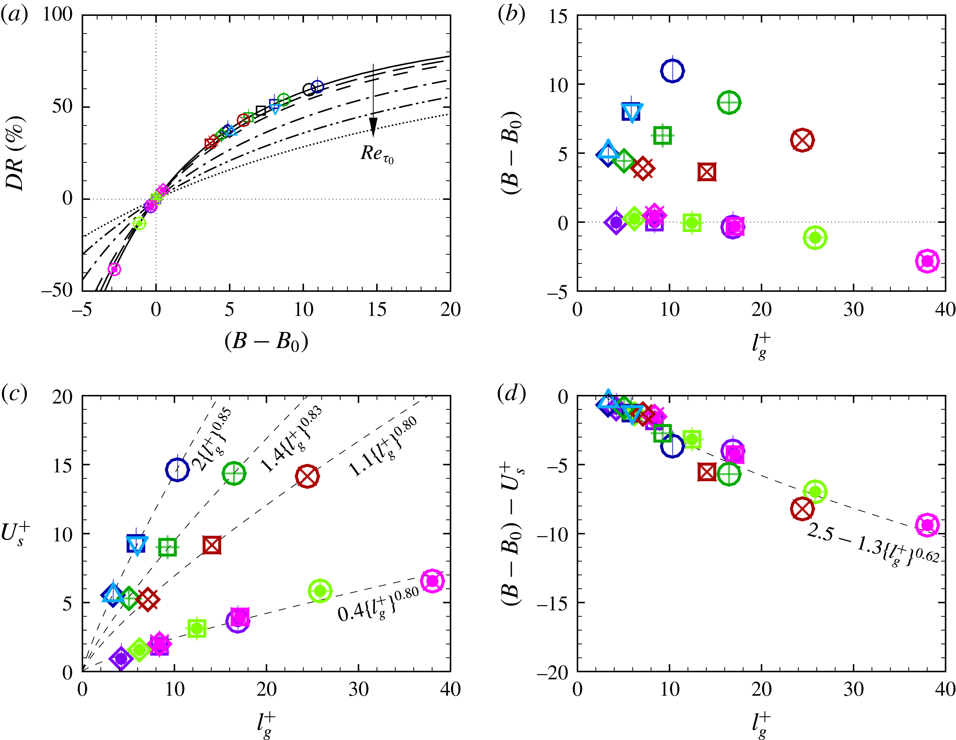
Figure 9(a) shows the magnitudes of
 $DR$
as a function of
 $(B-B_{0})$
from DNS of turbulent channel flow with SH longitudinal microgrooves or riblets in the present study, compared to the predictions of (5.3). The appearance of
 $\sqrt{C_{f_{0}}}$
in (5.3) leads to a degradation of
 $DR$
with increasing bulk Reynolds of the flow. The magnitude of this degradation, as predicted by (5.3), is consistent with the degradation of
 $DR$
observed in DNS when the
 $Re_{b}$
was increased from
 $3600$
to
 $7860$
. Figure 9(a) also shows the predictions of (5.3) for higher Reynolds number flows of practical interest, up to
 $Re_{b}=7.3\times 10^{8}$
(
 $Re_{\unicode[STIX]{x1D70F}_{0}}\approx 10^{6}$
). It can be seen that, for a given value of
 $(B-B_{0})$
, the drag reduction performance of SH longitudinal microgrooves and riblets degrades considerably with increasing bulk Reynolds number of the flow. Nevertheless, with a proper choice of the surface micro-texture geometry, drag reductions of up to 40–50 % should still be feasible with SH longitudinal microgrooves, assuming the liquid/gas interfaces in SH microgrooves remain stable and do not collapse.
Figure 9(b) shows the variation of
 $(B-B_{0})$
with the characteristic size of the microgrooves,
 $l_{g}^{+}$
, from DNS of turbulent channel flow with SH longitudinal microgrooves or riblets in the present study. Good agreement can be seen in the
 $(B-B_{0})$
values at different bulk Reynolds numbers for SH longitudinal microgrooves of size
 $g^{+0}\approx 14$
and
 $28$
at
 $\unicode[STIX]{x1D703}=-30^{\circ }$
, confirming the Reynolds number independence of
 $(B-B_{0})$
. However, the
 $(B-B_{0})$
values for SH longitudinal microgrooves with different protrusion angles do not collapse and show different trends compared to those for riblets.
To gain a better understanding of the source of these differences, one can decompose
 $(B-B_{0})$
into
 $$\begin{eqnarray}(B-B_{0})=\{U_{s}^{+}\}+\{(B-B_{0})-U_{s}^{+}\},\end{eqnarray}$$
where
 $\{U_{s}^{+}\}$
is the average streamwise slip velocity at the tip of the surface micro-texture, as shown in figure 8, representing all the drag reducing contributions to
 $DR$
arising from streamwise slip, while
 $\{(B-B_{0})-U_{s}^{+}\}$
represents all the drag enhancing contributions to
 $DR$
arising from spanwise slip, mean flow shear stresses developed due to the presence of the surface micro-texture and the faction of the flow rate through the surface micro-texture. Figure 9(c,d) shows the breakdown of
 $(B-B_{0})$
into
 $\{U_{s}^{+}\}$
and
 $\{(B-B_{0})-U_{s}^{+}\}$
from DNS of SH longitudinal microgroove and riblets in the present study. With riblets,
 $\{U_{s}^{+}\}$
follows the scaling
 $U_{s}^{+}\approx 0.4\{l_{g}^{+}\}^{0.8}$
for all microgroove depths, while with SH longitudinal microgrooves, it follows scalings which range from
 $U_{s}^{+}\approx 2.0\{l_{g}^{+}\}^{0.85}$
at
 $\unicode[STIX]{x1D703}=-30^{\circ }$
, to
 $U_{s}^{+}\approx 1.1\{l_{g}^{+}\}^{0.8}$
at
 $\unicode[STIX]{x1D703}=-90^{\circ }$
, indicating that with increasing protrusion angle, the scaling of
 $\{U_{s}^{+}\}$
with SH longitudinal microgrooves begins to approach that of riblets. The drag enhancing contributions represented by
 $\{(B-B_{0})-U_{s}^{+}\}$
, however, show a common scaling with both SH longitudinal microgrooves and riblets, as shown in figure 9(d), once again indicating that, aside from their magnitudes of streamwise surface slip, SH longitudinal microgrooves and riblets share a common mechanism of drag reduction. The collapse of the data from SH longitudinal microgrooves and riblets in figure 9(d) is not as good as the results shown in figures 2(k) and 3(b,d), due to the approximations used in the derivation in (5.3). Nevertheless, the characterization of
 $DR$
in terms of
 $(B-B_{0})$
given by (5.3), combined with the results shown in figure 9, provides a simple method for predicting the magnitude of drag reduction with micro-textured surfaces in high Reynolds number turbulent flows of practical interest.
6 Implications for design of more stable SH surfaces
The presence of a common mechanism of drag reduction with SH longitudinal microgrooves and riblets suggests that the two approaches can be combined synergistically to reduce the pressure loads on SH interfaces, and enhance their longevity and sustainability in turbulent flow environments.
Figure 10(a–c) shows the r.m.s. pressure fluctuations in turbulent channel flows with SH longitudinal microgrooves investigated in the present study. The presence of interface curvature at the protrusion angle of
 $\unicode[STIX]{x1D703}=-30^{\circ }$
leads to drops of 13 %, 15 % and 28 % in the magnitudes of r.m.s. pressure fluctuations at the wall with microgrooves of size
 $g^{+0}\approx 14$
,
 $28$
and
 $56$
, compared to same-size microgrooves with flat SH interfaces, respectively. The drops in instantaneous pressure fluctuations are even more dramatic, as shown in figure 10(d–g) for the case
 $g^{+0}\approx 14$
. The instantaneous pressure fluctuations on the micro-textured wall with SH longitudinal microgrooves at
 $\unicode[STIX]{x1D703}=-30^{\circ }$
are nearly a factor of two smaller than the micro-textured wall with SH longitudinal microgrooves at
 $\unicode[STIX]{x1D703}=0^{\circ }$
.
Turbulent pressure fluctuations in channel flow with SH longitudinal microgrooves: (a–c) r.m.s. turbulent pressure fluctuations; (d–g) contour plots of instantaneous turbulent pressure fluctuations on the channel boundaries for
 $g^{+0}\approx 14$
;
 $w^{+0}\approx 2$
and
 $\unicode[STIX]{x1D703}=0^{\circ },-30^{\circ },-60^{\circ },-90^{\circ }$
, respectively. Line types as in figure 4.

These results suggest that one can improve the stability of SH surfaces by developing hybrid designs of SH surfaces, in which the SH surface is embedded within the microgrooves of shallow (
 $\unicode[STIX]{x1D703}=-30^{\circ }$
) scalloped riblets. Indeed, this may be the design adopted by nature in shark scales, which has gone unnoticed to date.
7 Summary and conclusions
Skin-friction drag reduction with SH longitudinal microgrooves and riblets has been investigated by mathematical analysis and DNS in channel flow. An exact analytic expression is derived for the magnitude of drag reduction with micro-textured surfaces, which allows the net drag reduction to be decomposed into its constitutive elements. It is shown that in laminar or turbulent channel flow with any SH or riblet micro-texture pattern on the walls, five elements contribute to the net drag reduction: (i) the effective slip velocity at the wall, which augments the bulk velocity and allows a fraction
 $(U_{s}/U_{b})$
of the flow rate to flow inviscidly; (ii) modifications to the normalized structure of turbulent Reynolds shear stresses due to this augmentation of the bulk velocity by the effective slip velocity at the wall; (iii) other modifications to the normalized structure of turbulent Reynolds shear stresses in the presence of the wall micro-texture; (iv) modifications to the mean flow shear stresses due to the presence of the wall micro-texture; and (v) the flow rate through the wall micro-texture.
Comparison to DNS results in turbulent channel flow at
 $Re_{b}=3600$
(
 $Re_{\unicode[STIX]{x1D70F}_{0}}\approx 222$
) and
 $Re_{b}=7860$
(
 $Re_{\unicode[STIX]{x1D70F}_{0}}\approx 442$
) shows that SH longitudinal microgrooves and riblets share a common mechanism of drag reduction, in which 100 % of the drag reduction arises from effects (i) and (ii), namely, the effective slip velocity at the wall, and modifications to the normalized structure of turbulent Reynolds shear stresses due the presence of this effective slip velocity. All other modifications to the normalized structure of turbulent Reynolds shear stresses and the structure of the mean flow shear stresses due to the presence of the wall micro-texture, as well as the effect of the flow rate through the wall micro-texture, are drag enhancing, and follow common scalings for SH longitudinal microgrooves and riblets when expressed as a function of the characteristic size of the wall micro-texture,
 $l_{g}^{+}=\sqrt{A_{G}^{+}}$
.
It is shown that DNS studies at
 $Re_{\unicode[STIX]{x1D70F}_{0}}\approx 200$
properly represent the physics of drag reduction with micro-textured surfaces at higher Reynolds numbers. Extrapolation of drag reduction data from DNS to high Reynolds number flows of practical interest is discussed. It is shown that, for a given geometry and size of the surface micro-texture in wall units, there is significant degradation in the drag reduction performance of micro-textured surfaces with increasing Reynolds number of the flow.
Curved SH interfaces with small protrusion angle (
 $\unicode[STIX]{x1D703}=-30^{\circ }$
) are shown to reduce the r.m.s. and instantaneous pressure fluctuations on the SH interface compared to flat SH surfaces. This suggests that the longevity of SH surfaces in turbulent flow environments may be improved by using hybrid designs, in which the SH surface is embedded within the microgrooves of shallow (
 $\unicode[STIX]{x1D703}=-30^{\circ }$
) scalloped riblets.
Acknowledgements
This work was supported by an unrestricted grant from the M. R. Prince Foundation, and NSF XSEDE Allocation TG-CTS070067N. This support is gratefully acknowledged. The study has greatly benefited from suggestions by the anonymous referees. We thank the referees for this anonymous contribution.
Appendix A. Verification of numerical methods
A number of numerical tests were performed to verify the accuracy of the lattice Boltzmann methods and adequacy of the grid resolutions and domain sizes employed in the present study. These tests include (i) comparisons of lattice Boltzmann DNS to pseudo-spectral DNS in turbulent channel flow with smooth, no-slip walls; (ii) verification of grid independence of the results, by comparisons of lattice Boltzmann DNS results on successively refined grids in turbulent channel flows with SH longitudinal microgrooves with flat SH interfaces; (iii) verification of adequacy of the domain size, by comparisons of lattice Boltzmann DNS in small and large domain turbulent channel flows with SH longitudinal microgrooves with flat SH interfaces; and (iv) verification of curved interface boundary conditions, by comparisons of lattice Boltzmann DNS results to numerical simulations of Wang et al. (Reference Wang, Teo and Khoo2014) in laminar channel flows with SH longitudinal microgrooves and curved SH interfaces at various interface protrusion angles.
A.1 Comparisons to pseudo-spectral DNS in turbulent channel flow with smooth walls
All the simulations reported in the present study were performed using standard D3Q19, single relaxation time lattice Boltzmann methods (Succi Reference Succi2001), with grid embedding (Lagrava et al.
Reference Lagrava, Malaspinas, Latt and Chopard2012) employed in the near-wall region, between the domain boundaries and the buffer layer (
 $z^{+0}\approx 30$
), to improve the accuracy of the computations near the micro-textured walls.
The accuracy of the lattice Boltzmann DNS code in turbulent flow with smooth, no-slip walls was assessed by comparing its results, both with and without grid embedding, to pseudo-spectral DNS in turbulent channel flow. The studies were performed in channels of size
 $5h\times 2.5h\times 2h$
in the streamwise, spanwise and wall-normal directions, respectively. A constant flow rate was maintained in the channel during the course of all the simulations, corresponding to a bulk Reynolds number of
 $Re_{b}=3600$
. The lattice Boltzmann DNS without grid embedding was performed using uniform grid spacings of
 $\unicode[STIX]{x1D6E5}^{+0}\approx 2$
, which is the standard recommended resolution for DNS of turbulent wall-bounded flows with lattice Boltzmann methods (Lammers et al.
Reference Lammers, Beronov, Volkert, Brenner and Durst2006). The lattice Boltzmann DNS with grid embedding was performed with a grid refinement ratio of
 $GR=4$
, employed in the region between the domain boundaries and the buffer layer (
 $z^{+0}\approx 30$
), resulting in grid spacings of
 $\unicode[STIX]{x1D6E5}_{f}^{+0}\approx 0.5$
for
 $z^{+0}\lesssim 30$
, and
 $\unicode[STIX]{x1D6E5}_{c}^{+0}\approx 2$
for
 $z^{+0}\gtrsim 30$
, as shown in figure 1(b). The pseudo-spectral DNS was performed using uniform Fourier grids of size
 $\unicode[STIX]{x1D6E5}_{x}^{+0}\approx 8$
and
 $\unicode[STIX]{x1D6E5}_{y}^{+0}\approx 4$
in the streamwise and spanwise directions, respectively, and non-uniform Chebyshev grids of size
 $0.07\lesssim \unicode[STIX]{x1D6E5}_{z}^{+0}\lesssim 4.5$
in the wall-normal direction.
Summary of the simulations performed to assess the accuracy of numerical methods, grid independence of the results, and adequacy of the domain size. All tests were performed in turbulent channel flow at
 $Re_{b}=3600$
. PS and LB denote pseudo-spectral and lattice Boltzmann methods, respectively.
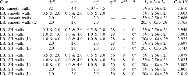
The skin-friction coefficients predicted by lattice Boltzmann DNS, with and without grid embedding, were within
 $0.1$
and
 $1\,\%$
of the values predicted by pseudo-spectral DNS, respectively, as shown in table 2. Similarly, the normalized profiles of mean streamwise velocities, turbulence intensities and Reynolds shear stresses predicted by lattice Boltzmann DNS, with and without grid embedding, were within 1 and 4 % of the results obtained from pseudo-spectral DNS, respectively, as shown in figure 11(a–c). These results indicate that the higher resolutions provided by grid embedding are not essential for lattice Boltzmann DNS in turbulent channel flows with smooth, no-slip walls. However, the higher resolutions offered by grid embedding in the near-wall region improve the accuracy of the simulations.
Effect of grid resolution and domain size on turbulence statistics in (a–c) turbulent channel flow with smooth, no-slip walls; (d–f) turbulent channel flow with SH longitudinal microgrooves of size
 $g^{+0}\approx 28$
,
 $w^{+0}\approx 4$
at protrusion angle of
 $\unicode[STIX]{x1D703}=0^{\circ }$
; (
 $g{-}i$
) turbulent channel flow with SH longitudinal microgrooves of size
 $g^{+0}\approx 56$
,
 $w^{+0}\approx 8$
at protrusion angle of
 $\unicode[STIX]{x1D703}=0^{\circ }$
: (a,d,g) mean velocity profiles; (b,e,h) turbulence intensities; (c,f,i) Reynolds shear stresses. (L) denotes simulations performed in large domains.
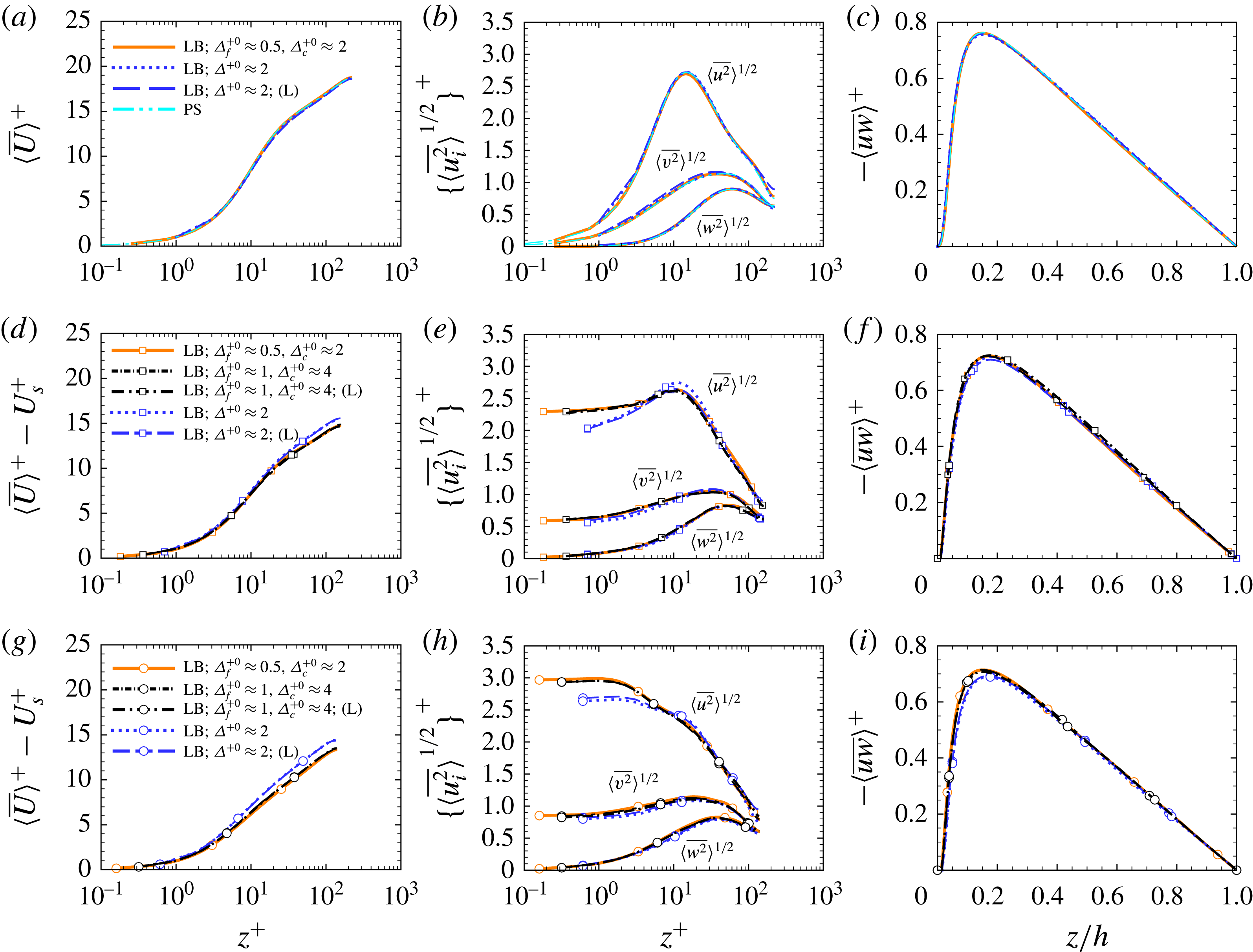
A.2 Need for grid embedding in flows with micro-textured surfaces and verification of grid independence of the results
With micro-textured surfaces, however, grid embedding becomes essential for obtaining accurate results. To demonstrate the need for grid embedding and verify the grid independence of the results, simulations both with and without grid embedding were performed in turbulent channel flows with SH longitudinal microgrooves of size
 $g^{+0}\approx 28$
,
 $w^{+0}\approx 4$
and
 $g^{+0}\approx 56$
,
 $w^{+0}\approx 8$
, at interface protrusion angle of
 $\unicode[STIX]{x1D703}=0^{\circ }$
, as shown in table 2. These simulations were also performed in channels of size
 $5h\times 2.5h\times 2h$
in the streamwise, spanwise and wall-normal directions, respectively, at a bulk Reynolds number of
 $Re_{b}=3600$
. The simulations without grid embedding were performed with uniform grid spacings of
 $\unicode[STIX]{x1D6E5}^{+0}\approx 2$
throughout the domain. The simulations with grid embedding were performed with a grid refinement ratio of
 $GR=4$
within the region
 $z^{+}\lesssim 30$
, and two different sets of grid resolutions, corresponding to
 $\unicode[STIX]{x1D6E5}_{f}^{+0}\approx 0.5$
,
 $\unicode[STIX]{x1D6E5}_{c}^{+0}\approx 2$
, and
 $\unicode[STIX]{x1D6E5}_{f}^{+0}\approx 1$
,
 $\unicode[STIX]{x1D6E5}_{c}^{+0}\approx 4$
, respectively, to verify the grid independence of the results.
The skin-friction coefficients obtained with grid spacings of
 $\unicode[STIX]{x1D6E5}_{f}^{+0}\approx 1$
,
 $\unicode[STIX]{x1D6E5}_{c}^{+0}\approx 4$
, were within 1.2 % and 1.7 % of those obtained with
 $\unicode[STIX]{x1D6E5}_{f}^{+0}\approx 0.5$
,
 $\unicode[STIX]{x1D6E5}_{c}^{+0}\approx 2$
, for flows with SH longitudinal microgrooves of size
 $g^{+0}\approx 28$
,
 $w^{+0}\approx 4$
and
 $g^{+0}\approx 56$
,
 $w^{+0}\approx 8$
, respectively, as reported in table 2. Similarly, the normalized profiles of mean streamwise velocities, turbulence intensities and Reynolds shear stresses obtained with grid spacings of
 $\unicode[STIX]{x1D6E5}_{f}^{+0}\approx 1$
,
 $\unicode[STIX]{x1D6E5}_{c}^{+0}\approx 4$
, were within 2.5 % of the results obtained with
 $\unicode[STIX]{x1D6E5}_{f}^{+0}\approx 0.5$
,
 $\unicode[STIX]{x1D6E5}_{c}^{+0}\approx 2$
, as shown in figure 11(d–i). These results demonstrate the grid independence of the results and adequacy of the grid spacings of
 $\unicode[STIX]{x1D6E5}_{f}^{+0}\approx 0.5$
,
 $\unicode[STIX]{x1D6E5}_{c}^{+0}\approx 2$
employed in all the simulations in the present study.
Without grid embedding, the predicted skin-friction coefficients differed from the values obtained with grid embedding, and grid spacings of
 $\unicode[STIX]{x1D6E5}_{f}^{+0}\approx 0.5$
,
 $\unicode[STIX]{x1D6E5}_{c}^{+0}\approx 2$
, by up to 10 %, as reported in table 2, while the normalized profiles of mean streamwise velocities, turbulence intensities and Reynolds shear stresses differed by up to 13 %, as shown in figure 11(d–i). These deviations show that grid spacings of
 $\unicode[STIX]{x1D6E5}^{+0}\approx 2$
do not provide an adequate grid resolution for lattice Boltzmann DNS of turbulent flows with a wall micro-texture.
The need for grid embedding in the presence of a surface micro-texture arises from the formation of sharp shear layers between the slip and no-slip regions at the tip of the surface microgrooves. These shear layers lead to sharp velocity gradients in the spanwise direction near the surface micro-texture. The effect of these gradients extends away from the walls to distances of the order of the width of the microgrooves. A fine grid, with grid spacings of the order of
 $\unicode[STIX]{x1D6E5}^{+0}\approx 0.5$
, is necessary to resolve the gradients near the micro-textured walls. Beyond a distance of
 $z^{+0}\approx 30$
, however, the spanwise gradients have weakened to the point that grid spacings of the order of
 $\unicode[STIX]{x1D6E5}^{+0}\approx 2$
can adequately resolve the weakened gradients.
These features can be verified by examining the one-dimensional energy spectra of turbulent velocity fluctuations,
 $E_{\unicode[STIX]{x1D6FC}\unicode[STIX]{x1D6FC}}^{+}$
, as shown in figure 12. When a coarse grid, of size
 $\unicode[STIX]{x1D6E5}^{+0}\approx 2$
, is used near the micro-textured walls, the inadequate grid resolution within the region
 $z^{+0}\lesssim 30$
leads to a pile up of turbulence kinetic energy in the one-dimensional energy spectra for spanwise wavenumbers
 $k_{y}^{+}\gtrsim 0.3$
, as shown in figure 12(e,f). Increasing the grid resolution to
 $\unicode[STIX]{x1D6E5}_{f}^{+0}\approx 0.5$
in this region, by employing grid embedding, resolves these issues and leads to disappearance of the energy pile-up, as seen in figure 12(e,f). Beyond a distance of
 $z^{+0}\approx 30$
from the walls, however, no pile up of energy is observed with
 $\unicode[STIX]{x1D6E5}^{+0}\approx 2$
, as seen in figure 12(k,l), indicating that grid spacings of
 $\unicode[STIX]{x1D6E5}_{c}^{+0}\approx 2$
provide adequate resolution for
 $z^{+0}\gtrsim 30$
.
A.3 Effect of domain size
The simulations reported in this study were all performed in channels of size
 $5h\times 2.5h\times 2h$
in the streamwise, spanwise and wall-normal directions, respectively. To assess the effect of domain size on the results, the simulations in base turbulent channel flow with smooth, no-slip walls, and in turbulent channel flows with SH longitudinal microgrooves of size
 $g^{+0}\approx 28$
,
 $w^{+0}\approx 4$
and
 $g^{+0}\approx 56$
,
 $w^{+0}\approx 8$
, with interface protrusion angle of
 $\unicode[STIX]{x1D703}=0^{\circ }$
, were repeated in channels of size
 $20h\times 10h\times 2h$
, as reported in table 2. A bulk Reynolds number of
 $Re_{b}=3600$
was maintained in the channel in all of these simulations. To reduce the cost of the computations, all the large domain simulations were performed either without grid embedding, at grid spacings of
 $\unicode[STIX]{x1D6E5}^{+0}\approx 2$
, or with grid embedding, at grid spacings of
 $\unicode[STIX]{x1D6E5}_{f}^{+0}\approx 1$
and
 $\unicode[STIX]{x1D6E5}_{c}^{+0}\approx 4$
, as shown in table 2.
Effect of grid resolution and domain size on one-dimensional energy spectra in (a,d,g,j) turbulent channel flow with smooth, no-slip walls; (b,e,h,k) turbulent channel flow with SH longitudinal microgrooves of size
 $g^{+0}\approx 28$
,
 $w^{+0}\approx 4$
at protrusion angle of
 $\unicode[STIX]{x1D703}=0^{\circ }$
; (c,f,i,l) turbulent channel flow with SH longitudinal microgrooves of size
 $g^{+0}\approx 56$
,
 $w^{+0}\approx 8$
at protrusion angle of
 $\unicode[STIX]{x1D703}=0^{\circ }$
. Line types as in figure 11.
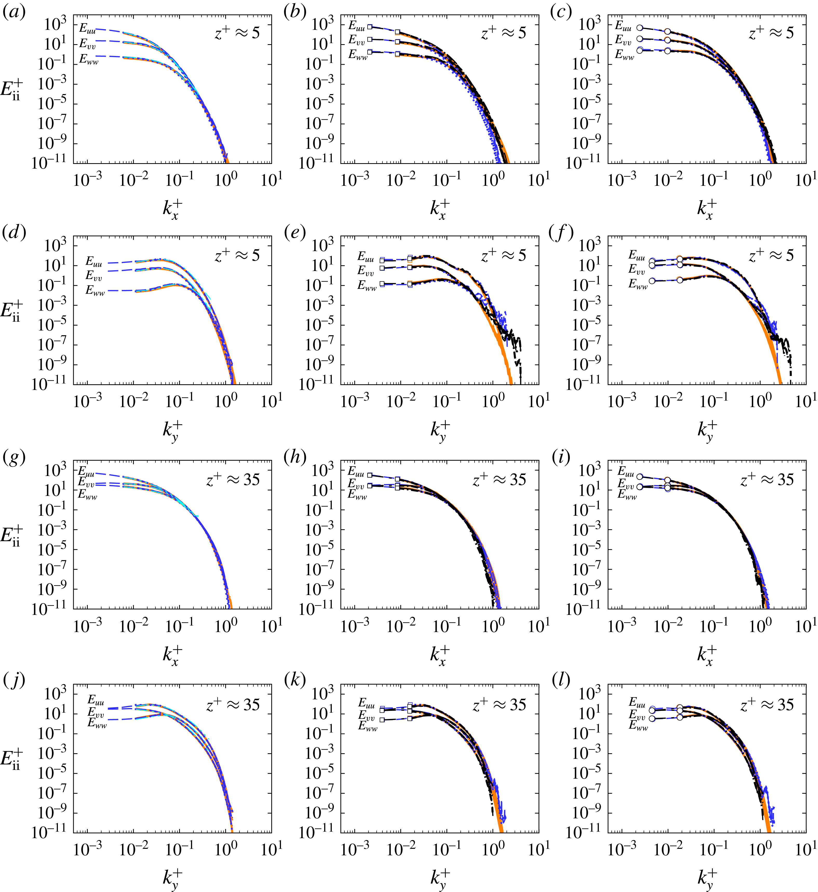
Effect of grid resolution and domain size on two-point correlations of velocity fluctuations in (a,d,g,j) turbulent channel flow with smooth, no-slip walls; (b,e,h,k) turbulent channel flow with SH longitudinal microgrooves of size
 $g^{+0}\approx 28$
,
 $w^{+0}\approx 4$
at protrusion angle of
 $\unicode[STIX]{x1D703}=0^{\circ }$
; (c,f,i,l) turbulent channel flow with SH longitudinal microgrooves of size
 $g^{+0}\approx 56$
,
 $w^{+0}\approx 8$
at protrusion angle of
 $\unicode[STIX]{x1D703}=0^{\circ }$
. (L) Denotes simulations performed in large domains.
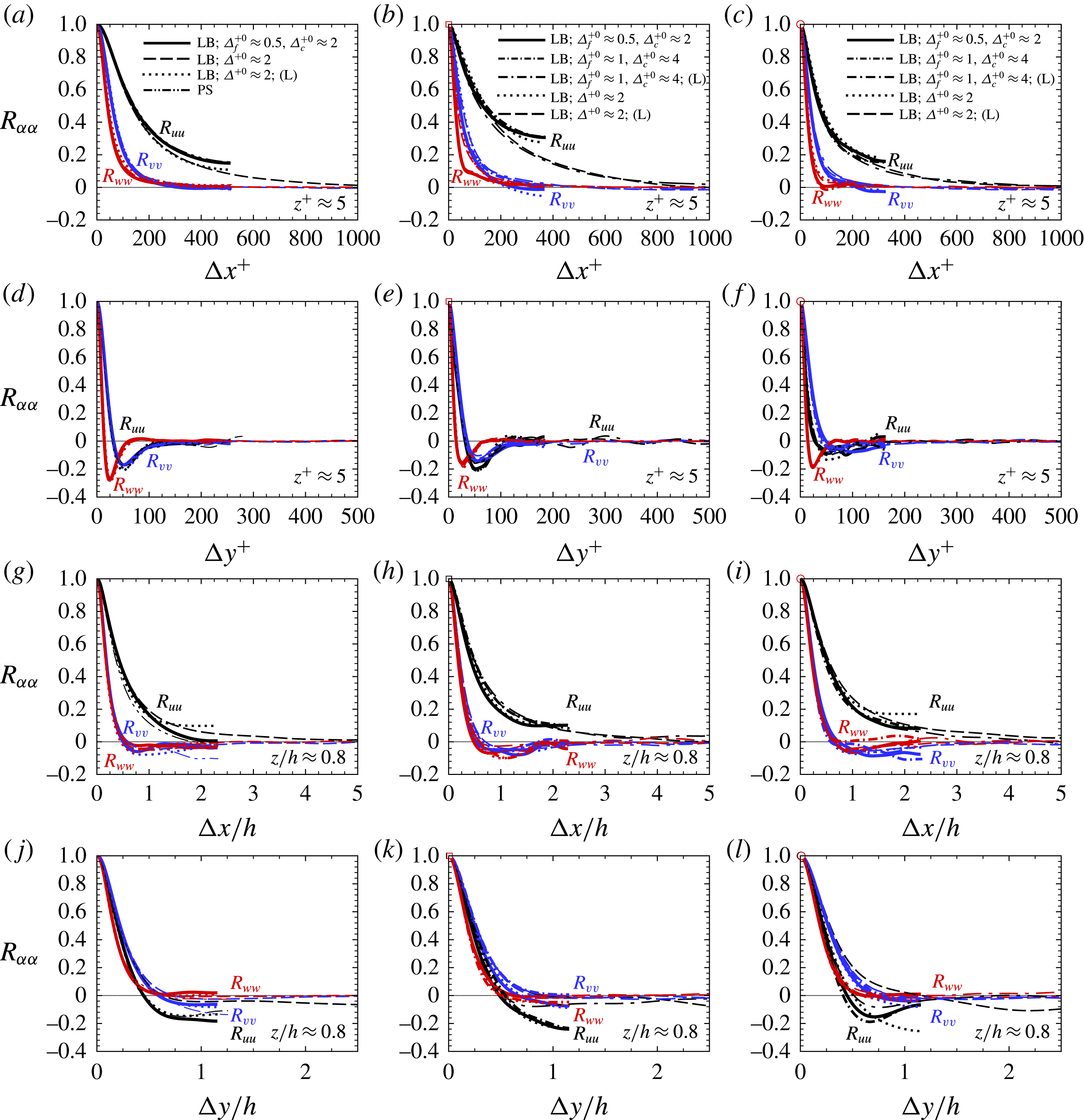
Verification of lattice Boltzmann DNS in laminar channel flow with SH longitudinal microgrooves and curved liquid/gas interfaces: (a)
 $L_{s}/h$
; (b)
 $U_{s}/U_{b_{0}}$
. ▵, ▿, DNS without grid embedding at
 $\unicode[STIX]{x1D6E5}/g=1/32$
and
 $\unicode[STIX]{x1D6E5}/g=1/64$
, respectively. ▫, ♢, DNS with
 $GR=4$
grid embedding at
 $\unicode[STIX]{x1D6E5}_{f}/g=1/32$
and
 $\unicode[STIX]{x1D6E5}_{f}/g=1/64$
, respectively. ○, analytical solution of Philip (Reference Philip1972); ——, numerical simulations of Wang et al. (Reference Wang, Teo and Khoo2014). All simulations performed at
 $Re_{b}=150$
in channels with SH longitudinal microgrooves of size
 $(g+w)/h=0.196$
and
 $g/w=1$
on both walls.
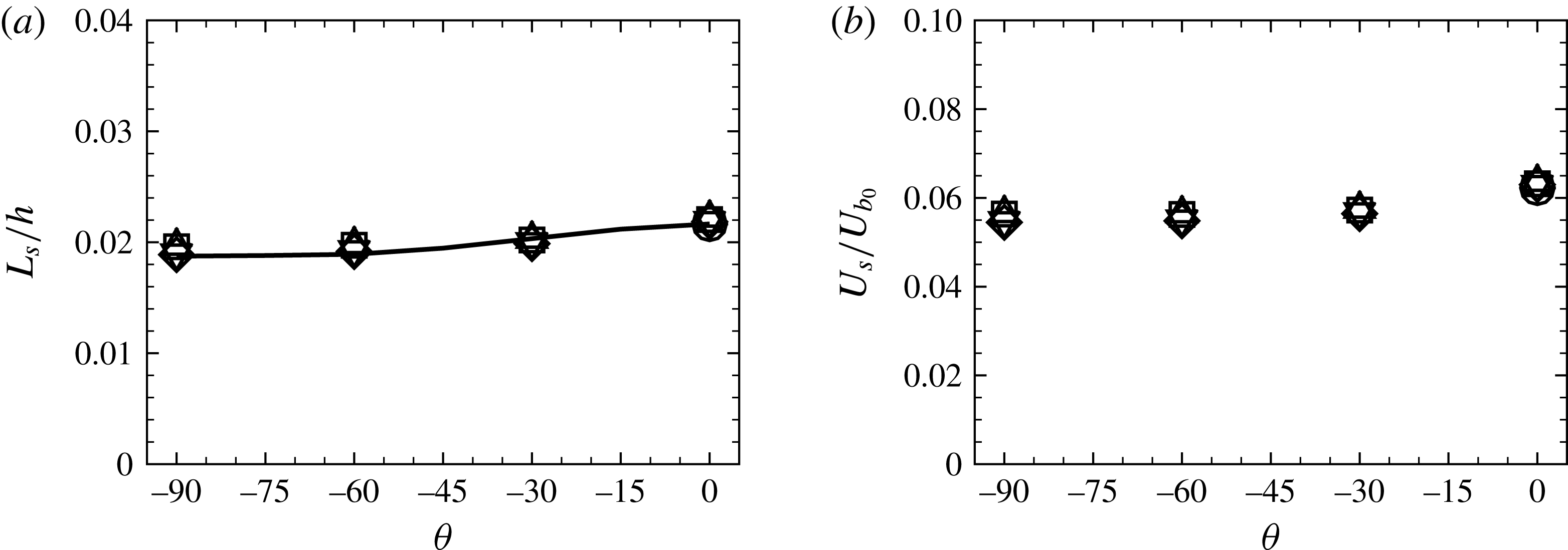
Comparison of DNS results in the small and large domains shows that the size of the domain has a negligible effect on the resulting skin-friction coefficients and turbulence statistics. The skin-friction coefficients obtained in the large domains were all within 0.5–1.2 % of the values obtained in the small domains with the same grid spacings, as shown in table 2. Similarly, the turbulence statistics and spectra in the large and small domains were in good agreement, as shown in figures 11 and 12. The largest differences in the turbulence statistics were observed in the streamwise turbulence intensities in the out layer (
 $z^{+}\gtrsim 100$
), where the values from the large domains could be higher than those in the small domains by up to 10 %, as shown in figure 11(b,e,h).
Figure 13 shows the two-point correlations of turbulent velocity fluctuations,
 $R_{\unicode[STIX]{x1D6FC}\unicode[STIX]{x1D6FC}}$
, in the large and small domains, at
 $z^{+}\approx 5$
and
 $z/h=0.8$
. In the large domains, the two-point correlations drop to zero at a separation of one half the domain lengths in both the near-wall region,
 $z^{+}\approx 5$
, and the core,
 $z/h=0.8$
. The two-point correlations in the smaller domains follow the trends in the larger domains, and drop to sufficiently low values at a separation of one half their domain lengths to ensure that the turbulence statistics are not affected, except for minor differences in the core region, as seen in figure 11. These results indicate the adequacy of the smaller domain size, employed in the present study.
A.4 Tests in laminar SH channel flow with curved SH interfaces
The accuracy of lattice Boltzmann DNS in dealing with curved liquid/gas SH interfaces was verified through comparisons of lattice Boltzmann DNS results, both with and without grid embedding, with results from numerical simulations of Wang et al. (Reference Wang, Teo and Khoo2014), performed using finite-element methods, in laminar channel flows with SH longitudinal microgrooves on the walls. In both studies, the liquid/gas interfaces in the SH longitudinal microgrooves were modelled as static, curved, shear-free boundaries, with the shape of the interface obtained from the solution of the Young–Laplace equation. The lattice Boltzmann simulations were performed in laminar channel flows at a bulk Reynolds number of
 $Re_{b}=150$
, with SH longitudinal microgrooves of size
 $(g+w)/h=0.196$
and
 $g/w=1$
on both walls, to match the geometric parameters of the longitudinal microgrooves in the simulations of Wang et al. (Reference Wang, Teo and Khoo2014). Static interface protrusion angles of
 $\unicode[STIX]{x1D703}=$
 $0^{\circ }$
,
 $-30^{\circ }$
,
 $-60^{\circ }$
,
 $-90^{\circ }$
, corresponding to interface curvatures of
 $\unicode[STIX]{x1D705}=0.0$
, 1.0, 1.732, 2.0 were investigated. The lattice Boltzmann simulations without grid embedding were performed at grid resolutions of
 $\unicode[STIX]{x1D6E5}/g=1/32$
and
 $\unicode[STIX]{x1D6E5}/g=1/64$
. The lattice Boltzmann simulations with grid embedding were performed with a grid refinement ratio of
 $GR=\unicode[STIX]{x1D6E5}_{c}/\unicode[STIX]{x1D6E5}_{f}=4$
, and grid resolutions of
 $\unicode[STIX]{x1D6E5}_{f}/g=1/32$
and
 $\unicode[STIX]{x1D6E5}_{f}/g=1/64$
, where the grid-embedding region extended from the domain boundaries to the tip of the longitudinal microgrooves. Figure 14 shows the resulting slip lengths,
 $L_{s}/h$
, and slip velocities,
 $U_{s}/U_{b_{0}}$
, computed by lattice Boltzmann DNS, compared to the results of Wang et al. (Reference Wang, Teo and Khoo2014). The results at different grid resolutions, both with and without grid embedding, are seen to be in agreement with each other and with the results reported by Wang et al. (Reference Wang, Teo and Khoo2014), demonstrating grid independence and accuracy of the results. Based on these studies, all the simulations reported in this work were performed with grid-embedding lattice Boltzmann DNS, with grids of size
 $1/112\leqslant \unicode[STIX]{x1D6E5}_{f}/g\leqslant 1/28$
and
 $\unicode[STIX]{x1D6E5}_{f}^{+0}\approx 0.5$
on the fine grid, and a
 $GR=\unicode[STIX]{x1D6E5}_{c}/\unicode[STIX]{x1D6E5}_{f}=4$
elsewhere, to ensure that both the dynamics of the flow near the curved boundaries and the turbulence dynamics are properly resolved.



