3.1. Characteristic scales of turbulence

In a turbulent mixing layer, the large-scale Kelvin–Helmholtz rollers and high- and low-speed structures are the largest coherent features which scale with the thickness of the mixing layer (Rogers & Moser Reference Rogers and Moser1994; Balaras, Piomelli & Wallace Reference Balaras, Piomelli and Wallace2001; Mungal Reference Mungal1995; Pirozzoli et al. Reference Pirozzoli, Bernardini, Marié and Grasso2015; Wang et al. Reference Wang, Wang and Chen2022). The momentum thickness ($\delta _\theta$) and vorticity thickness ($\delta _\omega$) are most commonly used to describe the thickness of the mixing layer. The former is defined as

(3.1)\begin{equation} \delta_\theta = \frac{1}{\rho_\infty \Delta U^2}\int_{-\infty}^{+\infty} \langle \rho \rangle \left( \Delta U/2-\tilde{u} \right)\left( \Delta U/2+\tilde{u} \right){\rm d}y. \end{equation}

The vorticity thickness is defined as $\delta _\omega =\Delta U/({\rm d}\langle u \rangle /{{\rm d}y})_{max}$ (Vreman et al. Reference Vreman, Sandham and Luo1996). In the self-similar periods, the two mixing layer thicknesses grow linearly with time (Rogers & Moser Reference Rogers and Moser1994; Pantano & Sarkar Reference Pantano and Sarkar2002; Wang et al. Reference Wang, Wang and Chen2022).

Figure 2 shows the ratio of the momentum thickness to the vorticity thickness for cases with convective Mach numbers $M_c = 0.2, 0.8, 1.8$. In the self-similar periods, the thickness ratio $\delta _\theta /\delta _\omega$ is nearly constant with time and decreases from 0.19 to 0.14 as the convective Mach number increases from 0.2 to 1.8. It has been found that the mean streamwise velocity profiles at different convective Mach numbers collapse very well when scaled with the free stream velocity difference $\Delta U$ and vorticity thickness $\delta _\omega$, and hence the vorticity thickness is used as an estimate of the integral scale of the mixing layer in the present work (Baltzer & Livescu Reference Baltzer and Livescu2020; Wang et al. Reference Wang, Wang and Chen2022).

Figure 2.

Time evolution of the thickness ratio $\delta _\theta /\delta _\omega$ at $M_c=0.2, 0.8$ and $1.8$. The vertical line segments mark the self-similar periods.

According to Kolmogorov's turbulence theory (Kolmogorov Reference Kolmogorov1941), the characteristic length scale of the smallest turbulent structures is given by the Kolmogorov length scale $\eta$, and the corresponding characteristic velocity is the Kolmogorov velocity $u_\eta =( \mu \epsilon /\rho )^{1/4}$. In figure 3(a), we plot the time evolution of the Kolmogorov length $\eta$ which is normalized by the vorticity thickness $\delta _\omega$ at $M_c=0.2$, $0.8$ and $1.8$. The normalized Kolmogorov length $\eta /\delta _\omega$ decreases exponentially with time in the self-similar periods, indicating an increasing scale separation between the small and integral scales of the turbulent mixing layer. As the convective Mach number increases, $\eta /\delta _\omega$ evidently increases, demonstrating that the compressibility suppresses the small-scale structures, and thus decreases the scale separation. As shown in figure 3(b), the normalized Kolmogorov velocity $u_\eta /\Delta U$ also decreases with time, while it slightly depends on the convective Mach number.

Figure 3.

Time evolution of (a) the normalized Kolmogorov length $\eta /\delta _\omega$ and (b) normalized Kolmogorov velocity $u_\eta /\Delta U$ at $M_c=0.2, 0.8$ and $1.8$. The length $\eta$, and velocity $u_\eta$ are evaluated at the centreline of the mixing layer. The vertical line segments mark the self-similar periods.

3.2. General properties of interfaces of LSSs

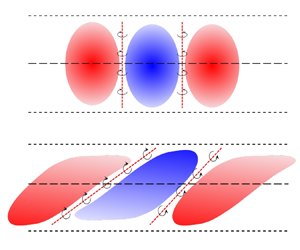
Figure 4 shows a two-dimensional schematic of high- and low-speed LSSs and small vortical structures near their interfaces. The shapes of high- and low-speed LSSs are reconstructed from the two-point correlations of fluctuating streamwise velocity reported by Wang et al. (Reference Wang, Wang and Chen2022). For ISL, edges of UMZs and TNTI, several identification approaches have been proposed to detect the location of these interfaces (Adrian et al. Reference Adrian, Meinhart and Tonkins2000; Kolář Reference Kolář2007; Fan et al. Reference Fan, Xu, Yao and Hickey2019). In the present work, we find that the isosurfaces of $u^\prime = 0$ provide a full three-dimensional description of the interfaces of two neighbouring high- and low-speed LSSs in a fluctuating velocity field. In this section, we report several general properties of the interfaces.

Figure 4.

Schematic of the high- and low-speed LSSs and small vortical structures near their interfaces in the (a) $x\unicode{x2013}y$ and (b) $z\unicode{x2013}y$ planes. The red and blue regions indicate the high- and low-speed LSSs, respectively. The red bold dashed line represents the interfaces superposed with small-scale vortices. The red arrow indicates the normal vector of the interface directed into low-speed region. The black circle with arrow indicates the small-scale vortex.

In figure 5(a), we plot five randomly selected streamwise velocity profiles. The instantaneous streamwise velocity $u/\Delta U$ in the vertical direction ($y$) presents a step-like profile with sharp changes in momentum indicating the existence of UMZs (highlighted in black-dashed ellipsoids), similar to that in turbulent boundary layers (De Silva et al. Reference De Silva, Philip, Hutchins and Marusic2017). In contrast, there is no evidence of UMZs in the profile of the fluctuating streamwise velocity $u^\prime /\Delta U$ which is constantly being used to signify the large-scale turbulent structures in turbulent shear flows, including turbulent boundary layer, jet and mixing layer (Lee et al. Reference Lee, Lee, Choi and Sung2014; Samie, Lavoie & Pollard Reference Samie, Lavoie and Pollard2021; Wang et al. Reference Wang, Wang and Chen2022). The corresponding profiles of the velocity gradient are shown in figure 5(b). We can find that the vertical gradients of the instantaneous streamwise velocity $u/\Delta U$ and fluctuating streamwise velocity $u^\prime /\Delta U$ almost overlap with each other. The magnitudes of the velocity gradients of $u/\Delta U$ and $u^\prime /\Delta U$ in high shear regions are much higher than (several times greater than) the maximum gradient of mean streamwise velocity. It is evident that the magnitude of positive gradients of the instantaneous and fluctuating streamwise velocity significantly exceeds that of negative velocity gradients. This is consistent with the observed behaviour of streamwise velocity gradients in turbulent boundary layers (De Silva et al. Reference De Silva, Philip, Hutchins and Marusic2017) and mixing layers (Fiscaletti et al. Reference Fiscaletti, Buxton and Attili2021).

Figure 5.

(a) Comparison between the vertical profiles of instantaneous streamwise velocity $u/\Delta U$ (red), fluctuating streamwise velocity $u^\prime /\Delta U$ (green) and mean streamwise velocity $\langle u \rangle /\Delta U$ (blue) at five equally spaced streamwise location from a snapshot for $M_c = 1.8$ at $\tau = 1750$, and (b) the corresponding profiles of the vertical gradients of them.

We present instantaneous visualizations of the spanwise vorticity $\omega _z$ in figure 6(a,b), the vertical vorticity $\omega _y$ in figure 6(c,d) and the streamwise vorticity $\omega _x$ in figure 6(e,f) at $M_c = 0.2$ and $1.8$. Here, the contour lines of $u^\prime /\Delta U=-0.1$ and $0.1$ are overlaid to display the high- and low-speed large-scale regions, instead of $u^\prime /\Delta U=0.0$, in order to give a qualitative impression of the velocity gradient which can be visualized by the distance between the two contour lines. The high shear regions (high-velocity gradients) are visualized by the colour contours of vorticity components. At $M_c=0.2$, the contour lines of $u^\prime /\Delta U=-0.1$ and $0.1$ obviously extend into the free stream, with characteristic sizes of the order of mixing layer thickness, which indicates the potential perturbations produced by the turbulence within the mixing layer. This observation is consistent with the previous study of a weakly compressible mixing layer by Almagro, Garciá-Villalba & Flores (Reference Almagro, Garciá-Villalba and Flores2017). It is convenient to utilize the TNTI as the outer edge of LSSs instead of the outer parts of the contour lines of $u^\prime /\Delta U=0$, similar to the outer edge of UMZs (De Silva et al. Reference De Silva, Philip, Hutchins and Marusic2017; Fan et al. Reference Fan, Xu, Yao and Hickey2019). Only the interfaces of LSSs within the turbulent region are studied in the following. At $M_c=0.2$, the contour lines of $u^\prime /\Delta U=-0.1$ and $0.1$ almost overlap with each other in the turbulent region, while there exists an evident separation between them at $M_c=1.8$, indicating the decrease of velocity gradient at points with $u^\prime /\Delta U=0$ as the convective Mach number increases. A significant proportion of the high shear regions (high vorticity) is concentrated in the near vicinity of the interfaces of LSSs, which is more obvious in figure 6(b,d,f) for higher convective Mach number $M_c=1.8$. At low convective Mach number $M_c=0.2$, the contour lines are complicated and tortuous with a concentration of small fragments, while they appear to be smoother and have fewer small structures at a higher convective Mach number $M_c=1.8$, indicating that the interfaces become stable as the convective Mach number increases. This stabilizing effect of compressibility on interfaces of LSSs resembles the behaviour of interfaces of UMZs with decreasing Reynolds number found by De Silva et al. (Reference De Silva, Philip, Hutchins and Marusic2017) in turbulent boundary layers. Meanwhile, we can see that the high shear regions are intermittently distributed on the continuous interfaces detected as isocontours of fluctuating streamwise velocity $u^\prime$. This is consistent with previous studies on edges of the UMZs in wall-bounded (De Silva et al. Reference De Silva, Philip, Hutchins and Marusic2017; Gul et al. Reference Gul, Elsinga and Westerweel2020) and free shear turbulence (Fiscaletti et al. Reference Fiscaletti, Buxton and Attili2021).

Figure 6.

Instantaneous visualization of contour lines of $u^\prime /\Delta U=-0.1$ and $0.1$ at (a,c,e) $M_c=0.2$ and (b,d,f) $M_c=1.8$, overlaid on colour contours of (a,b) spanwise vorticity $\omega _z$ in $x\unicode{x2013}y$ plane, (c,d) vertical vorticity $\omega _y$ in $x\unicode{x2013}z$ plane and (e,f) streamwise vorticity $\omega _x$ in $y\unicode{x2013}z$ plane.

In order to quantitatively illustrate the correlation between interfaces of LSSs (zero-$u^\prime$ isosurfaces) and high vorticity regions, we plot the joint probability density function ( p.d.f.) of the normalized vorticity components $\omega _i/\omega _{rms}$ and the normalized fluctuating streamwise velocity $u^\prime /\Delta U$ at convective Mach numbers $M_c =0.2$ in figure 7(a). It is found that the maximum of the p.d.f. for high values of $\omega _i/\omega _{rms}$ tends to appear at $u^\prime /\Delta U \approx 0$. The joint p.d.f.s of $(\omega _x/\omega _{rms},u^\prime /\Delta U)$ and $(\omega _y/\omega _{rms},u^\prime /\Delta U)$ are almost symmetric with respect to the line $\omega _x=0$ and $\omega _y=0$, respectively. However, the joint p.d.f. of ($\omega _z/\omega _{rms}$,$u^\prime /\Delta U$) is slightly negatively skewed (where $\omega _z=\partial {v}/\partial {x}-\partial {u}/\partial {y}$), indicating that the positive vertical gradient of the streamwise velocity occurs more frequently than the negative one, which is consistent with the observation in figure 5(b). As the convective Mach number increases from 0.2 to 1.8, the joint p.d.f. of ($\omega _z/\omega _{rms}$,$u^\prime /\Delta U$) significantly decreases along the abscissa, as shown in figure 7(b), indicating the stabilizing effect of compressibility on small-scale vortical structures in the turbulent mixing layer. The joint p.d.f.s of ($\omega _x/\omega _{rms}$,$u^\prime /\Delta U$) and ($\omega _y/\omega _{rms}$,$u^\prime /\Delta U$) at different convective Mach numbers resemble that of ($\omega _z/\omega _{rms}$,$u^\prime /\Delta U$) and are omitted here for the sake of brevity. The joint p.d.f. and visualization in figure 6 confirm that the interfaces of LSSs can be detected by zero-$u^\prime$ isosurfaces within the mixing layer. As previously mentioned, the UMZs and high- and low-speed LSSs arise from the observation of large-scale motions in different reference frames. The UMZs are typically observed in the laboratory frame within the instantaneous velocity field, whereas the LSSs are derived from the Reynolds-decomposed or fluctuating velocity field (de Silva et al. Reference de Silva, Hutchins and Marusic2016; Saxton-Fox & McKeon Reference Saxton-Fox and McKeon2017; Gul et al. Reference Gul, Elsinga and Westerweel2020; Heisel et al. Reference Heisel, De Silva, Hutchins, Marusic and Guala2021). The connection between the interfaces of UMZs and those of high- and low-speed LSSs remains an open question, and a preliminary analysis is offered in the Appendix A.

Figure 7.

Isocontour lines of (a) $\log _{10}$ p.d.f. ($\omega _i$,$u^\prime$) at $M_c=0.2$ and (b) $\log _{10}$ p.d.f. ($\omega _z$,$u^\prime$) for three different convective Mach numbers $M_c =0.2$, $0.8$ and $1.8$. Four contour lines at $-1,-2,-3$ and $-4$ are shown.

The orientation of the interfaces of LSSs can be distinguished by its unit normal vector defined as $\boldsymbol {n}= -\boldsymbol {\nabla } {u}^\prime /|\boldsymbol {\nabla } {u}^\prime |$, and its three components are equal to $\cos (\psi _i)$, where $\psi _i$ ($i=x$, $y$ and $z$) is the interface angle between the normal unit vector and three coordinate axes $x, y$ and $z,$ respectively. The unit normal vector of the interface is indicated by red arrows in figure 4. Figure 8 shows the p.d.f.s of the cosine of interface angles for low-speed LSSs, namely p.d.f. of $\cos (\psi _x)$, $\cos (\psi _y)$ and $\cos (\psi _z)$, at three different convective Mach numbers $M_c =0.2, 0.8$ and $1.8$. The p.d.f. of $\cos (\psi _x)$ shows two peaks near $\cos (\psi _x) = \pm 0.1$. The p.d.f. also shows a bimodal distribution with peaks at $-0.98$ and $0.92$ for $\cos (\psi _y)$, and $-0.95$ and $0.95$ for $\cos (\psi _z)$. These results indicate that most interfaces are approximately parallel to the streamwise direction, which is in accordance with the fact that LSSs are highly elongated in the streamwise direction. The most probable orientation of the interfaces is approximately $12^\circ$ with respect to horizontal for the peak of p.d.f. at $\cos (\psi _y)=-0.98$, and $23^\circ$ for the peak of p.d.f. at $\cos (\psi _y)=0.92$. The most probable orientation of $12^\circ$ is in good agreement with the average orientation of $10^\circ \unicode{x2013}15^\circ$ for the ISL reported in turbulent boundary layers (Squire Reference Squire2016; Heisel et al. Reference Heisel, De Silva, Hutchins, Marusic and Guala2021), which is crucial information for understanding these turbulent structures and holds significant importance for turbulence modelling. It is interesting to note that the peak of p.d.f. at $\cos (\psi _y) = -0.98$ is clearly higher than the peak at $\cos (\psi _y) = 0.92$, indicating a preferential orientation of the interfaces of LSSs in the negative vertical direction. A much weaker preferential orientation also can be found in the p.d.f. of $\cos (\psi _x)$. In addition, we find that the percentage of interfaces characterized by $\cos (\psi _y) <0$, oriented in the negative $y$-direction, is approximately 55 % of the total interfaces. In the incompressible mixing layer, Fiscaletti et al. (Reference Fiscaletti, Buxton and Attili2021) reported that ISLs with $\partial u /\partial y >0$ (equivalent to $\cos (\psi _y) <0$) are found between 60 % and 70 %. It should be pointed out that the ISLs are only part of the overall interfaces (de Silva et al. Reference de Silva, Hutchins and Marusic2016; Gul et al. Reference Gul, Elsinga and Westerweel2020; Heisel et al. Reference Heisel, De Silva, Hutchins, Marusic and Guala2021). These results show the inhomogeneity of the interfaces of LSSs. The p.d.f.s of $\cos (\psi _z)$ are completely symmetric with respect to the line $\cos (\psi _z)=0$, as shown in figure 8(c), since it is statistically homogeneous in the $z$-direction. The two peaks for all three p.d.f.s of interface orientation angle increase slightly with increasing convective Mach number from 0.2 to 1.8, especially for $\cos (\psi _x)$. The observations are consistent with the previous result that the large-scale high- and low-speed structures in the mixing layers are significantly streamwise elongated to have a smaller inclination angle at a higher convective Mach number (Wang et al. Reference Wang, Wang and Chen2022).

Figure 8.

The p.d.f. of the cosines of the angle between (a) the $x$-axis, (b) the $y$-axis, (c) the $z$-axis and the normal unit vector of the interfaces of LSSs at three different convective Mach numbers $M_c =0.2$, $0.8$ and $1.8$.

To highlight the correlation between interface orientation and the three vorticity components, the joint p.d.f. of the normalized vorticity components $\omega _j/\omega _{rms}$ and the cosine of the orientation angle $\cos (\psi _i)$ for low-speed LSSs is plotted in figure 9 for $M_c = 1.8$ at $\tau = 1750$. We can find that the spanwise and vertical vorticity components are highly dependent on the interface orientation, as shown in figures 9(f) and 9(h). As can be seen from figure 9(f), the positive and negative intense spanwise vorticities are largely concentrated in the first and third quadrants of the $\cos (\psi _y)\unicode{x2013}\omega _z$ plane, respectively, with two clear peaks around the most probable orientations of $\cos (\psi _y) \approx \pm 1$. Since the statistics presented here are solely based on the low-speed LSS, it is reasonable to conjecture that the negative and positive spanwise vorticities mainly result from shear between the high- and low-speed LSSs located above and below it, respectively, as shown by a schematic of the high- and low-speed LSSs in figure 4(a). The joint p.d.f. of ($\cos (\psi _z)$, $\omega _y/\omega _{rms}$) is shown in figure 9(h), and the high probability regions of positive and negative vertical vorticities fall in the second and fourth quadrants of $\cos (\psi _z)\unicode{x2013}\omega _y$ plane, with two peaks around the most probable orientations of $\cos (\psi _z) \approx \pm 1$. Similarly, we can expect that the negative and positive vertical vorticities mainly result from shear between the high- and low-speed LSSs located on the left- and right-hand side of it in the spanwise direction, respectively, as shown in figure 4(b). It is noteworthy that the joint p.d.f.s of ($\cos (\psi _i)$, $\omega _z/\omega _{rms}$) are distinctly asymmetric concerning the line $\omega _z/\omega _{rms} =0$ and skewed towards the negative side, suggesting a clear preference for negative spanwise vorticity. At convective Mach numbers $M_c = 0.2$, $0.8$, the joint p.d.f.s show similar behaviour and are not reproduced here for brevity. The interface orientation has a very modest effect on the intensity of the streamwise vorticity component, as shown in figures 9(a), 9(d) and 9(g). At all three convective Mach numbers, the joint p.d.f.s are almost unchanged with time during the self-similar region of the mixing layer.

Figure 9.

Isocontours of $\log _{10}$ p.d.f. ($\cos (\psi _i)$, $\omega _j$ ) for $M_c = 1.8$ at $\tau = 1750$. Four contour lines at $-1$, $-2$, $-3$ and $-4$ are shown.

In figure 10, we plot the average of normalized vorticity components $\omega _i/\omega _{rms}$ conditioned on the cosine of interface orientation $\cos (\psi _j)$ for low-speed LSSs. Only the results at $M_c = 1.8$ and $\tau = 1750$ are illustrated in figure 10 since the conditionally averaged vorticity components are similar at all three convective Mach numbers. We find that the conditionally averaged vorticity components are nearly independent of the interface orientation concerning the streamwise direction $\cos (\psi _x)$, due to the cancellation between positive and negative vorticity, which is also presented in figure 9(a–c). As shown in figure 10(b), the conditionally averaged spanwise vorticity $\langle \omega _z/\omega _{rms}|\cos (\psi _y)\rangle$ rapidly increases up to $1$ as $\cos (\psi _y)$ increases from $0.5$ to $1$, and decreases to $-1$ as $\cos (\psi _y)$ decreases from $-0.5$ to $-1$. The other two vorticity components $\langle \omega _x/\omega _{rms}|\cos (\psi _y)\rangle$ and $\langle \omega _y/\omega _{rms}|\cos (\psi _y)\rangle$ are almost independent of $\cos (\psi _y)$. From figure 10(c), it is interesting to find that $\langle \omega _y/\omega _{rms}|\cos (\psi _z)\rangle$ decreases linearly from $0.75$ to $-0.75$ as $\cos (\psi _z)$ increases from $-1$ to $1$. The streamwise vorticity $\langle \omega _x/\omega _{rms}|\cos (\psi _z)\rangle$ is also a linear function of $\cos (\psi _z)$ and is much smaller than the vertical vorticity. Here, $\langle \omega _z/\omega _{rms}|\cos (\psi _z)\rangle$ is small and always negative. Considering the dynamics of high- and low-speed LSSs and the definition of vorticity, one can expect that the large value of vorticity components $\omega _z=\partial v/\partial x-\partial u/\partial y$ and $\omega _y=\partial u/\partial z-\partial w/\partial x$ are caused by the vertical shear (see figure 4a) and the lateral shear (see figure 4b) of the adjacent LSSs, respectively.

Figure 10.

Average of normalized vorticity components $\omega _i/\omega _{rms}$ conditioned on the cosine of interface orientation $\cos (\psi _j)$ at $M_c = 1.8$ and at $\tau = 1750$.

3.3. Conditionally averaged velocity

The above results show that isosurfaces of $u^\prime = 0$ are suitable for representing the interfaces of high- and low-speed LSSs in the fluctuating velocity field. In order to obtain conditional statistics with respect to the distance from the interface, an interface coordinate ($\xi$) is introduced with its origin located at the interface, as indicated by red arrows in figure 4. The interface coordinate $\xi$ is set to be parallel to the unit normal vector defined as $\boldsymbol {n}= -\boldsymbol {\nabla } {u}^\prime /|\boldsymbol {\nabla } {u}^\prime |$, where $\xi >0$ directs into the low-speed region. Since the interface is a continuous three-dimensional surface, the unit normal vector can point along any direction within the three-dimensional space. The value of a flow variable in the interface coordinate $\xi$ is calculated from its neighbouring points in computational coordinates using trilinear interpolation. We denote the conditional average statistics in the interface coordinate by $\langle \,\cdot\, \rangle _I$. Only the interfaces of low-speed LSS within the turbulent region are studied in the present paper. An isoline of the r.m.s. vorticity magnitude $\omega _{rms}=0.01\Delta U/\delta _{\theta }^0$ is selected as the nominal threshold to identify the TNTI (Jahanbakhshi & Madnia Reference Jahanbakhshi and Madnia2016; Watanabe, Zhang & Nagata Reference Watanabe, Zhang and Nagata2018; Wang et al. Reference Wang, Wang and Chen2022).

Figure 11 shows the conditionally averaged profiles of the streamwise velocity across the internal interfaces of LSSs at different non-dimensional times $\tau = t\Delta U/\delta _\theta ^0$. We can observe a sharp rise of streamwise velocity across a thin thickness, which is similar to that observed at the edges of UMZs and the TNTI (Chauhan, Philip & Marusic Reference Chauhan, Philip and Marusic2014; de Silva et al. Reference de Silva, Hutchins and Marusic2016; Nagata et al. Reference Nagata, Watanabe and Nagata2018). These conditionally averaged profiles of the streamwise velocity exhibit large positive and negative peaks, and their magnitudes decrease linearly with the distance from the centre of the interface layer at the far-field region. There is a mild overshoot of conditionally averaged streamwise velocity near the interface, especially at lower convective Mach number $M_c=0.2$. It can be seen that the velocity jump at the interfaces grows rapidly with time, and reaches a maximum value in the transition stage at $\tau =125$ for low and moderate convective Mach numbers of $M_c=0.2$ and $0.8$, while at a later time of $\tau =250$ for $M_c=1.8$. Then, the conditionally averaged streamwise velocity decreases until reaching a gradual development stage in the self-similar period. The evolution process of interfaces at $M_c=0.2$ and $0.8$ during the transition stage is evidently faster than that at $M_c=1.8$, consistent with the overall behaviour of the development of the mixing layers.

Figure 11.

Conditionally averaged streamwise velocity profiles in the near vicinity of all detected internal interfaces at three times inside the transition stage and three times inside the self-similar stage of the mixing layer: (a) $M_c=0.2$; (b) $M_c=0.8$; (c) $M_c=1.8$. The red solid lines correspond to profile at the initial field.

Figure 12 shows the conditionally averaged streamwise velocity normalized by Kolmogorov velocity $u_\eta$ as a function of $\xi /\eta$ at $M_c=0.2$, $0.8$ and $1.8$ in the self-similar period. In this figure, $u_\eta$ and $\eta$ are the values computed at the centreline. The profiles show a fairly good collapse around the centre of the interface when normalized by the Kolmogorov scales, but they start to slightly deviate from each other in the far-field region. This result indicates that the internal interfaces of LSSs are dominated by the smallest structures characterized by the Kolmogorov length scale.

Figure 12.

Conditionally averaged streamwise velocity profiles at different times in the self-similar period for (a) $M_c=0.2$, (b) $M_c=0.8$ and (c) $M_c=1.8$. Profiles are normalized by the Kolmogorov length $\eta$ and velocity $u_\eta$.

The thickness of the ISL is typically estimated by projecting linear fits to the regions above and below the sharp velocity change on the profile of the conditionally averaged streamwise velocity, assuming the internal shear layer is a mixing layer (De Silva et al. Reference De Silva, Philip, Hutchins and Marusic2017; Chen et al. Reference Chen, Chung and Wan2020; Fiscaletti et al. Reference Fiscaletti, Buxton and Attili2021). The thickness can also simply be estimated as the distance between the negative and positive peaks of the streamwise velocity, giving rise to a slightly larger thickness than the former method (Eisma et al. Reference Eisma, Westerweel, Ooms and Elsinga2015; Hayashi et al. Reference Hayashi, Watanabe and Nagata2021; Heisel et al. Reference Heisel, De Silva, Hutchins, Marusic and Guala2021). Using the first method, the thickness of the interfaces within the mixing layer is found to be between $8\eta$ to $9\eta$, which is consistent with the typical internal shear layer thickness of $10\eta$ observed in the turbulent free-shear flows by Fiscaletti et al. (Reference Fiscaletti, Buxton and Attili2021) and in the outer region of the turbulent boundary layer by Eisma et al. (Reference Eisma, Westerweel, Ooms and Elsinga2015). The velocity jump, or velocity difference between the negative and positive peaks of the streamwise velocity is approximately $6 u_\eta$. The thickness and velocity jump are nearly independent of the convective Mach numbers, indicating the similarity of small-scale flow structures. We note that the conditional statistics are weakly dependent on momentum thickness Reynolds numbers $Re_\theta$ increasing from 3768 to 4798 at $M_c=0.2$ and from 3036 to 5232 at $M_c=1.8$, therefore, an even wider $Re$ range would be necessary to fully examine the appropriate characteristic scales in the future.

Figure 13 depicts the conditionally averaged streamwise velocity normalized by $\Delta U$ as a function of $\xi /\delta _\omega$ at $M_c=0.2$, $0.8$ and $1.8$. It is shown that the profiles collapse in a thinner layer around the centre of the interface, while they start to deviate from each other around the peaks. The velocity difference is approximately $0.1\Delta U$ and decreases with time or with an increase in the Reynolds number, which is in agreement with the results reported by Fiscaletti et al. (Reference Fiscaletti, Buxton and Attili2021) in turbulent free-shear flows. This result can be explained by the increasing scale separation as the Reynolds number increases with time; that is, the Kolmogorov velocity $u_\eta /\Delta U$ dominating the interfaces decreases with time, as shown in figure 3(b). For a mixing layer, the maximum velocity gradient is generally used to define its vorticity thickness as $\delta _\omega =\Delta U/({\rm d}\langle u \rangle /{{\rm d}y})_{max}$. When normalized by the $\Delta U$ and $\delta _\omega$, the maximum gradient of the mean streamwise velocity $({\rm d}\langle u \rangle /{{\rm d}y})_{max}$ for the mixing layer is approximately 1 and located at the centreline (Wang et al. Reference Wang, Wang and Chen2022). From figure 13, we can see that the normalized maximum gradient of the conditionally averaged streamwise velocity decreases from $-7$ to $-5$ as the convective Mach number increases from $0.2$ to $1.8$. This result suggests that the velocity gradient at the interfaces is almost one order of magnitude larger than that of the mean streamwise velocity, confirming the qualitative conclusion shown in figure 5(b). Another important result is that, under integral scales $\delta _\omega$ and $\Delta U$, the maximum gradient of the conditionally averaged streamwise velocity at the interfaces of LSSs is significantly suppressed by compressibility, and the relative reduction of the maximum gradient can reach up to 40 % for $M_c = 1.8$.

Figure 13.

Conditionally averaged streamwise velocity profiles at different times in the self-similar period for (a) $M_c=0.2$, (b) $M_c=0.8$ and (c) $M_c=1.8$. Profiles are normalized by the vorticity thickness $\delta _\omega$ and the velocity difference across the shear layer $\Delta U$.

Noting that the referenced existing studies in this section, including Eisma et al. (Reference Eisma, Westerweel, Ooms and Elsinga2015) and Fiscaletti et al. (Reference Fiscaletti, Buxton and Attili2021), calculate the velocity jump based on the average distribution of instantaneous velocity obtained at the internal shear layer (as the interface of UMZs). In contrast, our velocity jump is determined by the average fluctuating velocity at the interface of LSSs. Although the two velocity jumps exhibit some degree of agreement, noticeable differences exist in the average of fluctuating velocities at the interface of UMZs and the interface of LSSs, as shown in the Appendix A.

3.4. Effect of interface orientation

In § 3.2, we found that the orientation angle has an obvious influence on the shear strength (vorticity). The conditional statistics are computed separately for the leading, trailing and side edges to investigate the dependence on the interface orientation. The leading and trailing edges are defined as $\cos (\psi _y)<-0.5$ and $\cos (\psi _y)>0.5$, respectively. These definitions are based on the value of the interface angle ($\psi _y$), instead of $\psi _x$ used in previous works on TNTI, taking into account that the LSSs are highly elongated in the streamwise direction like a baguette. Similarly, the side edge is defined as $|\cos (\psi _z)|>0.5$, where the absolute value of the angle is considered because of homogeneity in the spanwise direction. It is worth noting that the selection of the interface angle criterion $\cos (\psi _c)=0.5$ is similar to the works of Zhang, Watanabe & Nagata (Reference Zhang, Watanabe and Nagata2019) and is a critical value beyond which the magnitude of conditionally averaged spanwise vorticity $\langle \omega _z/\omega _{rms}|\cos (\psi _y)\rangle$ rapidly increases, as shown in figure 10. The sensitivity of the results to the interface angle criterion $\cos (\psi _c)$ will be discussed in the following.

The influence of the orientation angle on the conditionally averaged streamwise velocity is shown in figure 14. The distance from the interface is normalized by the vorticity thickness of the mixing layer $\delta _\omega$. It is clearly seen that velocity jump strongly depends on the interface orientation. The magnitude of the streamwise velocity jump is greater at the leading edge than that at the entire edge, but smaller at the trailing edge. At the side edge, the streamwise velocity is slightly larger than that of the entire edge. The peak position of the profile weakly depends on the interface orientation, and the overshoot is more obvious at the trailing edge. A zoomed-in view of the same area of the interface layer is provided for all three convective Mach numbers. The interface orientation effect appears more clearly in the zoomed-in insets of figure 14, indicating that the magnitude of the velocity gradients at the leading edge is significantly higher than that at the trailing edge. On the other hand, the zoomed region of figure 14 reveals that the velocity gradient at different interface orientations decreases as the convective Mach number increases from $M_c=0.2$ to $1.8$.

Figure 14.

Conditionally averaged streamwise velocity at different edges for (a) $M_c=0.2$, (b) $M_c=0.8$ and (c) $M_c=1.8$. The enlarged views near the centre are shown in the insets.

The conditionally averaged profiles of the vertical velocity at different interface orientations are presented in figure 15. The vertical velocity is found to have a stronger dependence on the interface orientation and unexpectedly changes sign near the trailing edge. Near the leading edge and side edge, the vertical velocity is negatively correlated with the streamwise velocity, which is consistent with the scenario of $Q$2 events (defined by $\langle u^\prime \rangle _I <0$ and $\langle v^\prime \rangle _I >0$) on the low-speed side ($\xi >0$) and $Q$4 events (defined by $\langle u^\prime \rangle _I >0$ and $\langle v^\prime \rangle _I <0$ ) on the high-speed side ($\xi <0$). The $Q$2 and $Q$4 events contribute significantly to the negative Reynolds shear stress and the positive turbulence production (Wallace Reference Wallace2016; Arun et al. Reference Arun, Sameen, Srinivasan and Girimaji2019; Wang et al. Reference Wang, Wang and Chen2022). The vertical velocity at the trailing edge is smaller than that at the leading and side edges, inferring a degree of stabilizing of the interface here. At $M_c=0.2$ and $0.8$, the vertical velocity near the trailing edge is positive in the high-speed region ($\xi <0$) and negative in the low-speed region ($\xi >0$), which is inconsistent with $Q$2 and $Q$4 events, while it changes sign away from the centre of the interface. At a high convective Mach number $M_c=1.8$, it is interesting to observe that the vertical velocity at the trailing edge has a plateau between $\xi /\delta _\omega =-0.01$ and $0.01$.

Figure 15.

Conditionally averaged vertical velocity at different edges for (a) $M_c=0.2$, (b) $M_c=0.8$ and (c) $M_c=1.8$.

Figure 16(a–c) shows the conditionally averaged profiles of vertical velocity at the trailing edge identified using different values of interface angle criterion $|\cos (\psi _c)| =0.2$, $0.5$ and $0.8$. We can find that the vertical velocity at the trailing edge is very sensitive to the values of interface angle criterion $\psi _c$. At the small interface angle criterion with $|\cos (\psi _c)| =0.2$, the trailing edge vertical velocity is positive in the low-speed region, and it presents a clear jump at high convective Mach number $M_c=1.8$. As the interface angle criterion increases to $|\cos (\psi _c)| =0.8$, the trailing edge vertical velocity tends to be negative in the low-speed region, and the maximum jump occurs at low convective Mach number $M_c=0.2$. This scenario is consistent with the signature of $Q1$ events (defined by $\langle u^\prime \rangle _I >0$ and $\langle v^\prime \rangle _I >0$) on the high-speed side ($\xi <0$) and $Q$3 events (defined by $\langle u^\prime \rangle _I <0$ and $\langle v^\prime \rangle _I <0$ ) on the low-speed side ($\xi >0$). The $Q$1 and $Q$3 events contribute to the positive Reynolds shear stress and the negative turbulence production (Wallace Reference Wallace2016; Arun et al. Reference Arun, Sameen, Srinivasan and Girimaji2019; Wang et al. Reference Wang, Wang and Chen2022). The conditionally averaged vertical velocity at the leading edge at $M_c=1.8$ is displayed in figure 16(d) for comparison. The profiles are almost coincident for different interface angle criteria. The streamwise velocity for the three interface orientations is insensitive to the choice of the interface angle criterion $\psi _c$ and is not reproduced here for brevity. The mechanism behind this phenomenon will be further revealed in the next section based on the analysis of small-scale turbulent structures near the interface. Based on the above results, it can be suggested that, on average, the downward high-speed LSS (with $\langle u^\prime \rangle _I >0$ and $\langle v^\prime \rangle _I <0$) impinges on the upward low-speed LSS (with $\langle u^\prime \rangle _I <0$ and $\langle v^\prime \rangle _I >0$) at the leading edge, such that the high-speed structure rides over the low-speed structure, as illustrated in figure 4(a). Similar to the analysis by Eisma et al. (Reference Eisma, Westerweel, Ooms and Elsinga2015) on boundary layers, this compression process at the leading edge implies that vorticity stretching occurs in the spanwise ($z$) direction over this interface, which maintains a higher velocity jump and a sharp interface. While at the trailing edge, the downward high-speed LSS deviates from the upward low-speed LSS on average, indicating extensive strain in the $x\unicode{x2013}y$ plane. This results in a weaker velocity jump or shear. This speculative explanation will be verified by the analysis of turbulent structures near the interface in the next section.

Figure 16.

Conditionally averaged vertical velocity at the trailing edge identified using different values of interface angle criterion at (a) $M_c=0.2$, (b) $M_c=0.8$ and (c) $M_c=1.8$, compared with (d) that at the leading edge at $M_c=1.8$. The legend is the same for all plots.

3.5. Small-scale structures

We now focus on the small-scale structures near the interface which have been found to be dominated by the Kolmogorov scale. Figure 17 compares the conditional average of the r.m.s. vorticity magnitude $\omega _{rms}$ near the leading, side and trailing edges at convective Mach numbers $M_c=0.2$, $0.8$ and $1.8$. The r.m.s. vorticity magnitude $\omega _{rms}$ is normalized by $(\Delta U/\delta _\omega )$. The distance from the interface, $\xi$, is normalized by the centreline $\eta$ on the top horizontal axis and by $\delta _\omega$ on the bottom horizontal axis. The normalized r.m.s. vorticity magnitude $\langle \omega _{rms} \rangle _I /(\Delta U/\delta _\omega )$ is almost uniform far from the interface and begins to increase rapidly towards the centre of the interface. There is a significant dependence on the interface orientation. In the velocity jump region, $\langle \omega _{rms} \rangle _I /(\Delta U/\delta _\omega )$ is smallest near the trailing edge and largest near the leading edge, consistent with the effect of interface orientation on the velocity jump shown in figure 14. On the contrary, $\langle \omega _{rms} \rangle _I /(\Delta U/\delta _\omega )$ is smallest near the leading edge and largest near the trailing edge outside the velocity jump region. Compared with the entire edge, the r.m.s. vorticity magnitude is amplified at the leading edge and attenuated at the trailing edge. As the convective Mach number increases, $\langle \omega _{rms} \rangle _I /(\Delta U/\delta _\omega )$ decreases rapidly at the three interface orientations, indicating that the small-scale vortical structures are suppressed significantly by compressibility at the interface.

Figure 17.

Conditional average of the r.m.s. vorticity magnitude $\omega _{rms}$ at different edges at (a) $M_c=0.2$, (b) $M_c=0.8$ and (c) $M_c=1.8$.

More details on the small-scale structures have been investigated using the second invariant of velocity gradient tensor, namely the $Q$-criterion, proposed by Hunt, Wray & Moin (Reference Hunt, Wray and Moin1988). This technique was originally developed for incompressible flow and is applicable to compressible flow when the second invariant is obtained for the deviatoric part of velocity gradient tensor (Kolář Reference Kolář2009), $Q = 1/2(\varOmega _{ij}\varOmega _{ij}-S_{ij}S_{ij})$, where $\varOmega$ and $S$ are the antisymmetric and symmetric components of the deviatoric part of the velocity gradient tensor, respectively. According to the definition, a positive value of $Q$ indicates that the flow is locally dominated by vortex motion, and a negative value indicates regions dominated by shear strain. Figure 18 shows the conditionally averaged profiles of $Q$ at different interface orientations, where $Q$ is normalized by $(\Delta U/\delta _\omega )^2$. We can find that there is a sharp drop in $\langle Q \rangle _I/(\Delta U/\delta _\omega )^2$ as the distance from the interface increases. This implies that the interface is dominated by vortex motion with $\langle Q \rangle _I > 0$ in a small range. Near the leading and side edges, the vortex-dominated region is flanked by strain-dominated regions with two negative peaks located at $\xi /\eta \approx \pm 7$. While at the trailing edge, $\langle Q \rangle _I/(\Delta U/\delta _\omega )^2$ is always positive and two smaller positive peaks appear at $\xi /\eta \approx \pm 12$. As the convective Mach number increases, the magnitude of $\langle Q \rangle _I/(\Delta U/\delta _\omega )^2$ decreases dramatically at the three interface orientations, which is similar to the behaviour of the r.m.s. vorticity magnitude in figure 17. The observations from figures 17 and 18 confirm that the small-scale vortices are intermittently distributed and clustered to the interfaces of LSSs. Furthermore, they suggest that the effect of compressibility on the mixing layer is more pronounced at the interfaces of LSSs. In other words, compressibility stabilizes the interfaces of LSSs, providing valuable insights into the compressibility suppression mechanism.

Figure 18.

Conditionally averaged second invariant of velocity gradient tensor $Q$ at different edges for (a) $M_c=0.2$, (b) $M_c=0.8$ and (c) $M_c=1.8$.

To obtain a more complete picture of the small-scale turbulent structures, the two-dimensional average velocity field is calculated with conditional averaging of the velocity field around points on the leading or trailing edges of low-speed LSSs. The conditional averaging is performed in a rectangular subregion with local coordinates ($r_x, r_y, r_z$) along the coordinate system ($x,y,z$) used in the simulation and the origin located at the sampling point ($r_x=0, r_y=0, r_z=0$) in the flow. Figure 19 shows the velocity vector of average flow and contours of $\langle Q \rangle _I/(\Delta U/\delta _\omega )^2$ in the $r_x\unicode{x2013}r_y$ plane conditioned on the leading and trailing edges at $M_c=0.2$ and $1.8$, superimposed with the corresponding streamlines. For the leading edge, the averaged flow exhibits a shear layer pattern with two parallel flows inclined at an angle of approximately $45^\circ$ with respect to the streamwise direction. A region with large positive $\langle Q \rangle _I$ has an elliptical shape with its major axis along the interface and minor axis perpendicular to the interface. Two regions with negative $\langle Q \rangle _I$ appear above and below the region of positive $\langle Q \rangle _I$ region. As shown by the streamlines in figures 19(a) and 19(c), a vortical motion is formed at the centre of the shear layer, extending a large distance in the streamwise direction, indicating the effect of large-scale motions on the shear layer. The flow patterns at the leading edge are very similar to each other for low and high convective Mach numbers $M_c=0.2$ and $1.8$. A similar average flow pattern has been observed around ISLs in homogeneous isotropic turbulence (Watanabe et al. Reference Watanabe, Tanaka and Nagata2020) and turbulent planar jets (Hayashi et al. Reference Hayashi, Watanabe and Nagata2021), as well as around TNTIs in turbulent planar jets (Elsinga & da Silva Reference Elsinga and da Silva2019). Interestingly, figures 19(b) and 19(d) show that, for the trailing edge, the vortical motion centred at the interface becomes weaker, since the flow away from the interface is dominated by large-scale rotation characterized by large-scale circular streamlines, instead of parallel shear flow, particularly at low convective Mach number $M_c=0.2$. This result clearly shows that the high- and low-speed LSSs depart from each other at the trailing edge. Meanwhile, there are two saddle point flow patterns along the interface at $r_x/\delta _\omega =\pm 0.15$ and $\pm 0.2$ for $M_c=0.2$ and $1.8$, respectively.

Figure 19.

Velocity vector of average flow and contours of $\langle Q \rangle _I/(\Delta U/\delta _\omega )^2$ in the $r_x\unicode{x2013}r_y$ plane conditioned on the (a,c) leading and (b,d) trailing edges at (a,b) $M_c=0.2$ and (c,d) $M_c=1.8$. The corresponding streamlines are displayed with black bold solid lines. The red bold solid line represents the $\langle u^\prime \rangle _I=0$ line. The blue arrow indicates the normal vector of the interface directed into low-speed region. The contour cutoff level is $-0.02$ to $0.1$.

Elsinga & Marusic (Reference Elsinga and Marusic2010) investigated the universality of small-scale turbulence by evaluating the average flow pattern in the eigenframe defined by the eigenvectors of the rate of the strain tensor. They found very similar average flows around the vorticity vector in different turbulent flows, including turbulent boundary layer, turbulent channel flow and homogenous isotropic turbulence. Their average flows are also quite similar to those in figures 19(a) and 19(c). The shearing in the $r_x\unicode{x2013}r_y$ plane is composed of two velocity gradients $\partial u / \partial y$ and $\partial v / \partial x$. It can result from either a pure strain (a saddle point flow pattern) or a layered shear flow with a single non-zero velocity gradient, see figure 3 of Elsinga & Marusic (Reference Elsinga and Marusic2010). The flow pattern is a combination of pure strain and layered shear. Furthermore, the layered shear flow has the potential to develop secondary Kelvin–Helmholtz instability, resulting in secondary Kelvin–Helmholtz vortices (Smyth Reference Smyth2003; Fritts et al. Reference Fritts, Wang, Lund and Thorpe2022). The secondary Kelvin–Helmholtz vortices can be observed in the instantaneous flow visualizations in figure 6. As shown in figure 19, the layered shear dominates the average flow pattern near the leading edge with a secondary Kelvin–Helmholtz vortex located at the centre, while the dominance is weakened near the trailing edge due to the lower level of shear (see figure 14).

In the topological methodology introduced by Chong, Perry & Cantwell (Reference Chong, Perry and Cantwell1990), the small-scale structures of the velocity gradient tensor are examined through an analysis of its invariants. Detailed background information regarding the topological methodology is available in Chong et al. (Reference Chong, Perry and Cantwell1990), Cantwell (Reference Cantwell1992) and Ooi et al. (Reference Ooi, Martin, Soria and Chong1999). As demonstrated by Fiscaletti et al. (Reference Fiscaletti, Buxton and Attili2021), the intense shear layers in a spatially developing mixing are primarily governed by a ‘stable-focus/stretching’ flow topology. As shown in figure 19, the streamline pattern of the average flow at the leading edge is consistent with the flow topology referred to as ‘stable-focus/stretching’, signifying the dominance of vortex stretching in the spanwise ($z$) direction. This is consistent with the result of Fiscaletti et al. (Reference Fiscaletti, Buxton and Attili2021). On the other hand, the streamline pattern at the trailing edge corresponds to the flow topology termed ‘unstable-focus/compressing’, indicating the presence of vortex compression in the spanwise ($z$) direction. These results corroborate our analysis of the effect of interface orientation in § 3.4.

Based on the understanding of turbulent structures near the interface, we try to explain the sensitivity of vertical velocity on the interface orientation, as observed in figures 15 and 16. We plot the contours of $\langle v^\prime \rangle _I / \Delta U$ in the $r_x\unicode{x2013}r_y$ plane conditioned on the trailing edge identified with different values of interface angle criterion $\psi _c$ in figure 20. The results are only shown for $M_c=1.8$ because they are qualitatively similar for different convective Mach numbers. The preceding results have shown that the spanwise vorticity $\omega _z=\partial v/\partial x-\partial u/\partial y$ is strongly correlated with the interface orientation $\cos (\psi _y)$, as shown in figure 10. On average, the larger the $|\cos (\psi _c)|$, the larger the magnitude of spanwise vorticity $\omega _z$, and the stronger the shear at the interface. As seen in figure 20, the conditionally averaged field of vertical velocity is featured by two regions with different scales. One is the large-scale positive $\langle v^\prime \rangle _I$ region on the low-speed side and negative $\langle v^\prime \rangle _I$ region on the high-speed side far away from the interface (red solid line), which become smaller as the interface angle criterion $|\cos (\psi _c)|$ increases. The other one is a small-scale $\langle v^\prime \rangle _I$ region induced by the vortical structure at the origin, which is magnified as $|\cos (\psi _c)|$ increases. The latter dominates the average flow near the trailing edge at $|\cos (\psi _c)|=0.8$, which generates the $Q$1 events ($\langle u^\prime \rangle _I >0$ and $\langle v^\prime \rangle _I >0$) and $Q$3 events ($\langle u^\prime \rangle _I <0$ and $\langle v^\prime \rangle _I <0$).

Figure 20.

Velocity vector of average flow and contours of $\langle v^\prime \rangle _I / \Delta U$ in the $r_x\unicode{x2013}r_y$ plane conditioned on the trailing edge identified with different values of interface angle criterion: (a) $|\cos (\psi _c)| =0.2$; (b) $|\cos (\psi _c)| =0.5$; (c) $|\cos (\psi _c)| =0.8$ at $M_c=1.8$. The red bold solid line represents the $\langle u^\prime \rangle =0$ line. The blue arrow indicates the normal vector of the interface directed into low-speed region.

The above results confirm the explanation in § 3.4 that the downward high-speed LSS impacts the upward low-speed LSS at the leading edge and they depart from each other at the trailing edge, then resulting in a higher shear at the leading edge and a weaker shear at the trailing edge, respectively. What is of great importance is that the explanation is consistent with the phenomenon of large-scale amplitude modulation of the small-scale structures in turbulent boundary layers (Marusic et al. Reference Marusic, Mathis and Hutchins2010; Mathis et al. Reference Mathis, Hutchins and Marusic2011; Agostini & Leschziner Reference Agostini and Leschziner2014) and mixing layer (Wang et al. Reference Wang, Wang and Chen2022): the small-scale vortical structures are amplified at the top of low-speed LSS, which is directly associated with high-shearing motions, and the small-scale fluctuations are attenuated beneath the low-speed LSS.

3.6. Compressibility

For compressible flow, the velocity divergence $\varTheta$ serves as an excellent indicator of the local compressibility. Figure 21 shows the conditionally averaged velocity divergence $\langle \varTheta \rangle _I$ at different interface orientations for three Mach number cases, where $\langle \varTheta \rangle _I$ is normalized by $\Delta U/\delta _\omega$. At low and moderate convective Mach numbers $M_c=0.2, 0.8$, a gentle positive peak can be found within the interface layer at three interface orientations, which indicates that a fluid expansion is induced by the vortical structures. The peak value at $M_c=0.8$ is nearly 10 times larger than the value at $M_c=0.2$. The velocity divergence $\langle \varTheta \rangle _I$ is smallest near the trailing edge and largest near the leading edge, similar to the behaviour of rotation strength (positive $\langle Q \rangle _I$) at the trailing and leading edges, as shown in figure 18. At high turbulent Mach number $M_c=1.8$, the velocity divergence $\langle \varTheta \rangle _I$ exhibits two positive peaks near the leading and side edges at $\xi /\eta \approx \pm 3$. Between the two peaks, the fluid is slightly compressed at the leading edge, which is qualitatively similar to that observed near the TNTIs (Rossmann et al. Reference Rossmann, Mungal and Hanson2002; Zhou et al. Reference Zhou, He and Shen2012; Nagata et al. Reference Nagata, Watanabe and Nagata2018). A larger positive peak of $\langle \varTheta \rangle _I$ is observed near the trailing edge compared with the leading edge. Away from the interface, the velocity divergence $\langle \varTheta \rangle _I$ is mildly negative, indicating that the LSSs are compressive at $M_c=1.8$.

Figure 21.

Conditionally averaged velocity divergence at different edges for (a) $M_c=0.2$, (b) $M_c=0.8$ and (c) $M_c=1.8$.

Figure 22 shows the velocity vector of average flow and contours of the normalized velocity divergence $\langle \varTheta \rangle _I / (\Delta U/\delta _\omega )$ in the $r_x\unicode{x2013}r_y$ plane conditioned on the leading and trailing edges at $M_c=0.2$ and $1.8$. At $M_c=0.2$, there are no negative levels of the contour for $\langle \varTheta \rangle _I$ near the interface, implying that the flow is expansive on average near the leading and trailing edges. Close to the leading edge, the positive region of $\langle \varTheta \rangle _I$ has a similar shape to the small-scale vortical structure, while the positive regions mainly reside in shear-dominated regions near the trailing edge, as shown in figures 22(a) and 22(b). Due to the lack of samples, the results are not statistically stable far away from the interface with regard to LSSs. At a higher convective Mach number $M_c=1.8$, a narrow compression region passes through the centre of a small-scale vortical structure with an inclination angle of $45^\circ$ with respect to the interface and links two strong compression motions in the shear-dominated regions away from the leading edge. There are two expansion regions on both sides of the shock-like compression region. Moreover, we observe that expansion motion dominates the average flow near the trailing edge at $M_c=1.8$.

Figure 22.

Velocity vector of the average flow and contours of $\langle \varTheta \rangle _I / (\Delta U/\delta _\omega )$ in the $r_x\unicode{x2013}r_y$ plane conditioned on the (a,c) leading and (b,d) trailing edges at (a,b) $M_c=0.2$ and (c,d) $M_c=1.8$. The red bold solid line represents the $\langle u^\prime \rangle _I =0$ line. The blue arrow indicates the normal vector of the interface directed into the low-speed region.