1. Introduction

My goal in this article is to develop and defend a general theory of epistemic risk within the epistemic utility framework. In light of the growing influence of decision-theoretic approaches to epistemology, it is natural to consider what role risk will play in the normative assessment of an agent’s credence function. To date, there is very little literature on this topic.Footnote ¹

I make some fairly basic assumptions about epistemic value. For illustrative purposes, we will proceed under the fiction that an agent’s selection of a credence function may be treated as an epistemic act such that the rationality of that act can be evaluated using the tools of ordinary decision theory. One epistemic act is preferable to another if it increases expected epistemic utility, where epistemic utility is given in terms of a scoring rule. Scoring rules measure the accuracy of an agent’s credence function. Thus, accuracy is our primary epistemic commodity.

If we are to develop a theory of risk within the framework of epistemic utility, the riskiness of a credence function should reflect an agent’s exposure to potential losses in accuracy. The theory should be alethic, so to speak. We will see that following this line of inquiry, the shape of an agent’s epistemic risk function reflects her relative sensitivity to different types of graded error. In simple cases, this implies that the shape of the risk function reflects an agent’s attitude toward the relative cost of increasing inaccuracy in the direction of false positive (type I) mistakes against the cost of increasing inaccuracy in the direction of false negative (type II) mistakes. On larger sample spaces, the risk function reflects an agent’s attitude to increasing inaccuracy in the direction of every possible outcome. Meanwhile, the curvature of the risk function encodes attitudes toward marginal changes in accuracy and local sensitivity to error.

To develop a measure of epistemic risk that captures the preceding idea, I propose an approach inspired by Rothschild and Stiglitz’s (Reference Rothschild and Stiglitz1970) measure of economic risk in terms of stochastic dominance. On my approach, one credence function is riskier than another if it is a mean-preserving spread of it, and the least risky credence function is the one that guarantees a particular accuracy score regardless of the state of the world. We will see that for credence functions, mean-preserving spreads in accuracy are equivalent to certain changes in expectation and that a plausible measure of risk, therefore, is the difference in expectation from the risk-free credences. In simple cases, this measure has a very natural interpretation in terms of the difference between the agent’s best and worst outcomes.

Following Grunwald and Dawid (Reference Grunwald and Dawid2004), I use the term ‘general entropy’ to refer to the expected accuracy of a credence function evaluated with respect to itself (we will see why below). As a result, the notion of epistemic risk I advocate is also a measure of entropic change. Indeed, the main formal contribution of this article is a duality theorem connecting epistemic risk and general entropy, which will be established in section 5: namely, that under very general conditions risk is a scaled reflection of general entropy. That is,

$\mathrm{risk}+\mathrm{entropy}=k\mathrm{.}$

This is a fruitful link between risk and information entropy. From every risk function we may derive a unique scoring rule, and the agent’s attitude to different types of error will determine the shape of her score. For example, if she considers the different error costs to be equal, her score will evaluate equally changes in accuracy in the direction of each outcome. If such an agent seeks to minimize epistemic risk, she will identify a uniform prior by applying the Laplacean principle of indifference (POI). However, the uniform prior minimizes epistemic risk only if the different types of error are treated equally. This is quite a substantial assumption, and a version of it appears in Pettigrew’s (Reference Pettigrew2016a) accuracy argument for the POI. More generally, the relationship between risk and general entropy suggests that there exists a family of indifference principles (rather than a unique POI) each reflecting a different way of evaluating the error costs of a prospective credence function. This highlights the normative commitments that come with endorsing an uninformative or flat prior. The agent’s risk profile, therefore, is in an important sense epistemically central. Once we know what it is, we can determine the appropriate measure of risk, the associated entropy, and the scoring rule.

The article proceeds as follows. Section 2 provides an overview of competing approaches one might use to develop a theory of epistemic risk, focusing in particular on the difference between alethic and modal conceptions of risk. In section 3, I describe the relevant formal concepts. In section 4, I develop the theory of epistemic risk for a simple case. In section 5, I articulate the normative attitudes to the cost of error implied by the location, shape, and curvature of an agent’s epistemic risk function. In section 6, I develop the duality between risk and entropy. Section 7 extends the approach to more general sample spaces. Finally, section 8 explores the relationship between epistemic risk, the selection of priors, and the Laplacean POI.

2. Background

In financial analyses the expression ‘value at risk’ denotes the quantity (in monetary terms) that a firm or financial portfolio, say, stands to lose. As we seek to develop a theory of epistemic risk, we can begin by asking a related question: When an agent adopts a credence function that the theory deems risky, what is the value under risk? I can think of two approaches we might take to the epistemic value in jeopardy: the alethic approach, which I will develop, where the value is accuracy, and the modal approach, developed recently in Pritchard (Reference Pritchard2017), where the value is knowledge. The alethic approach is especially appropriate to Bayesian epistemology, since finely grained beliefs can approach the truth to various degrees, whereas the modal approach may be best suited for traditional full-belief approaches, in which justification plays a central role.

3. Formal Framework

Following the literature, I adopt the useful fiction that an agent is able to choose between competing credence functions. Thus, credence functions will be the object of risk, and ultimately we seek to compare and rank them in terms of their riskiness. As suggested above, it is natural in this framework to suppose that one credence function is riskier than another if the agent stands to lose more in terms of accuracy or that variability in accuracy outcomes is greater. This resembles in some respects Peirce’s (Reference Peirce1879/1967) notion of the “economy of research.”Footnote ⁴ I develop the theory carefully below. The remainder of this section provides a directed introduction to the relevant formal concepts.

I assume that an epistemically rational agent should adopt as her credence function a probability distribution whose expected inaccuracy is at least as low as any alternative distribution she might adopt.Footnote ⁵ This is Joyce’s (Reference Joyce1998) norm of gradational accuracy. It captures the veritist spirit in a context of fine-grained subjective uncertainty. Minimizing expected inaccuracy plays a role in epistemic utility theory similar to what maximizing expected utility plays in ordinary decision theory. To measure inaccuracy, we use a scoring rule. This is a two-place function $s:\{0,1\}\times [0,1]\to ℝ$, denoted by s_v (p(h)), that measures the inaccuracy of the probability assigned to h when the true outcome is v, where $v=1$ if h is true and 0 otherwise.

Three properties of scoring rules will be relevant to my argument: truth-directedness, continuity, and strict propriety. Truth-directedness implies that s ₁(p) is a decreasing function of p and s ₀(p) is an increasing function of p.Footnote ⁶ Thus, moving closer toward the actual truth-value cannot make an agent worse off. Continuity implies that s ₁ and s ₀ are continuous functions of p. This enables us to avoid arbitrarily small changes in credence leading to large changes in accuracy. Before we define strict propriety, we need to introduce one more concept. The expected inaccuracy of a probability distribution is the expectation of s_v (p) evaluated with respect to the agent’s beliefs, $b=b\left(h\right)$. In the binary case, this is

(1)$\begin{array}{}& E_b\left[s_v\right(p\left)\right]={\mathrm{bs}}_1\left(p\right)+(1-b)s_0\left(p\right)\mathrm{.}\end{array}$

If this equation is (uniquely) minimized at $b=p$, the score is (strictly) proper. This means that a coherent agent can do no better in expectation, from the perspective of minimizing inaccuracy, than to adopt as her credence function the probability distribution that corresponds to her sincere degrees of belief.

One more property will be relevant to my argument. It is not presupposed in any of the theorems—rather, it will inform our discussion of the rationality of different attitudes to epistemic risk. We say that s_v is 0/1 symmetric if, given two probabilities for h, p(h) and q(h), that are identical except that $p\left(h\right)=1-q\left(h\right)$, then $s_1\left(p\right(h\left)\right)=s_0\left(q\right(h\left)\right)$.

I assume that an agent’s normative attitudes to risk, if they are to be found anywhere, must be reflected in the prior the agent deems appropriate. As a result, in developing a measure of epistemic risk, we set aside for now considerations of updating and ask: regardless of one’s evidence about a proposition, what structural features make one credence function riskier than another? Of course, it is also important to consider what makes one update riskier than another. Equivalently, how much epistemic risk might be justified by the agent’s evidence? These are questions about dynamic epistemic risk, and I pursue them in subsequent work.Footnote ⁷

4. Epistemic Risk: The Simple Case

Consider an agent formulating a credence p(h) about a single proposition h. Regardless of h’s content, we know that the agent’s inaccuracy decreases as her credences get closer to the truth and that it increases as they get further away from it. Since s ₁ is continuous and decreasing on [0, 1] with $s_1\left(1\right)=0$, and s ₀ is continuous and increasing on [0, 1] with $s_0\left(0\right)=0$, the intermediate value theorem guarantees that there exists a point of intersection p* for which $s_1\left(p^{*}\right)=s_0\left(p^{*}\right)$. 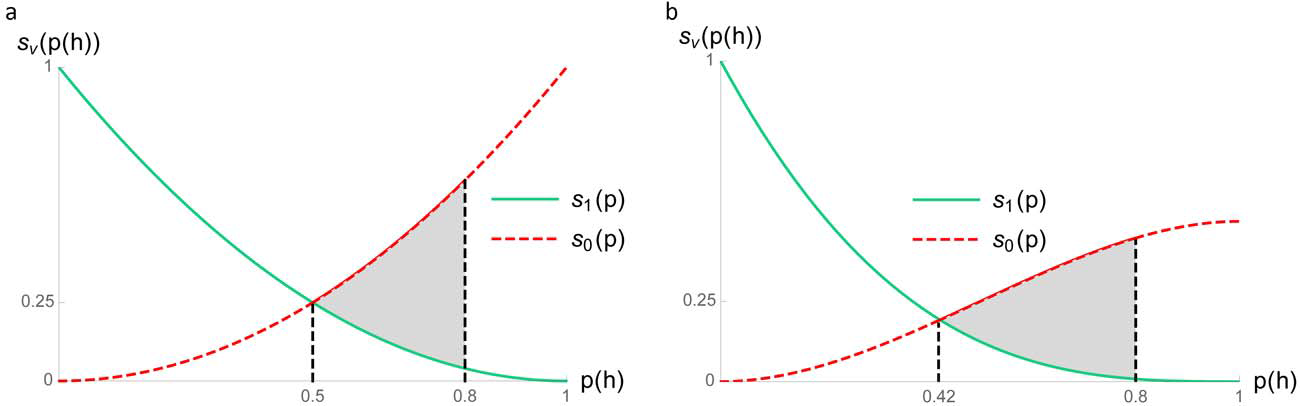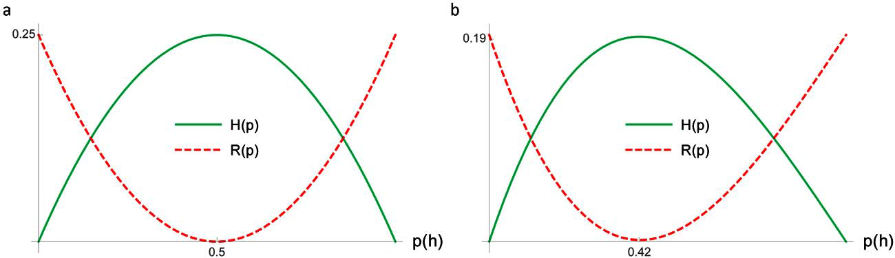For $0/1$ symmetric scores, this is 0.5. For asymmetric scores it may be something else. Figure 1 illustrates this situation. Figure 1a depicts a symmetric score, whereas figure 1b depicts an asymmetric one.

Figure 1.

Risk-free probability p*, where $s_1\left(p^{*}\right)=s_0\left(p^{*}\right)$: a, symmetric score; b, asymmetric score.

The point p* may be thought of as the least risky probability assignment in the following sense: if the agent’s credence for h is given by p*, her inaccuracy will be the same regardless of the actual truth-value for h. As a result, she knows with certainty how inaccurate she will be, even before she learns whether h is true or false.

It is natural to think of a guarantee in one’s outcome as implying an absence of risk. Indeed, this is the purpose of ordinary insurance: to charge a premium for guaranteeing a particular outcome (and, in turn, removing risk)—hence, ‘risk premium’. The outcome in insurance contexts is given in monetary terms. Here the same idea applies, but the relevant commodity is accuracy, and therefore the outcome is given in inaccuracy as measured by a scoring rule. Informally, therefore, we might identify p* as the least risky probability in the sense that it guarantees a certain inaccuracy score, regardless of outcome. Since the choice of scale in constructing a risk measure is arbitrary, we may call p* the risk-free credence and define it more formally as follows.

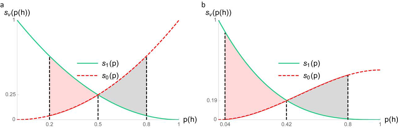
Now suppose that the agent has a stronger credence for h, say 0.8. Then if h is true, her inaccuracy will be very low, but if h is false, her inaccuracy will be quite high. Since $p\left(h\right)=0.8$ creates an opportunity for the agent (the probability of doing better) together with a corresponding potential cost (the probability of doing worse), it is in this sense a riskier credence relative to p* on the alethic approach. A natural measure for this increase in risk is the spread between s ₁ and s ₀, as depicted by the shaded areas in figure 2, because this quantity increases monotonically with shifts of probability to the tails of the risk-free distribution.Footnote ⁸ Figure 2a depicts the increase in risk from a $0/1$ symmetric score’s risk-free credence, whereas figure 2b depicts the increase in risk from an asymmetric score’s risk-free credence.

Figure 2.

Increasing epistemic risk: a, symmetric measure of risk; b, asymmetric measure of risk.

Notice, however, that it is less sensible to speak about one credence function being riskier than another if we vary the number of possible outcomes in the sample space. With three outcomes instead of two, the risk-free probability would occur where $s_1\left(p\right)=s_2\left(q\right)=s_3(1-p-q)$. Assuming a $0/1$ symmetric score, this would be the uniform distribution $p=q=1/3$. So to evaluate the riskiness of a credence function over three outcomes, we should measure the “spread” from the risk-free distribution for this larger space (we will see how to do this later). In light of these remarks, we may define a risk measure for the single proposition case as follows.

Epistemic risk. Given a single proposition h and a risk-free credence p*, the risk associated with investing credence $p<p^{*}$ in h is

$R\left(p\right)={\int }_p^{p^{*}}\left|s_1\right(t)-s_0\left(t\right)|\mathrm{dt}\mathrm{.}$

For $p>p^{*}$, the bounds of integration are reversed. For $p=p^{*}$, $R\left(p\right)=0$.

Provided the scoring rule is continuous, the risk function will be likewise continuous. Its local maxima will occur at $p\left(h\right)=0$ and $p\left(h\right)=1$. Since the scoring rule must be monotonically decreasing as the credence approaches the true value, risk monotonically increases away from the risk-free credence.Footnote ⁹

5. Risk and Normativity

Any move away from the risk-free credence threatens to increase inaccuracy, by either increasing confidence in h when it is false or decreasing confidence in h when it is true. Whether one deems the direction important reflects a substantial normative attitude toward the cost of approaching different types of error. As p(h) goes up, one risks increasing inaccuracy in the direction of a false positive (type I) error. Meanwhile, as p(h) goes down, one risks increasing inaccuracy in the direction of a false negative (type II) error.Footnote ¹⁰ It is doubtful that the only rational attitude to these types of error is indifference (as $0/1$ symmetry suggests). Being solely concerned with the truth, as Gibbard (Reference Gibbard2008) points out, does not commit one to a particular way of valuing accuracy. As a result, we want our measure of risk (and associated scoring rule) to reflect different trade-offs that agents might make between moving toward either type of error.

For example, h could be the outcome of a coin toss, where unit increases in inaccuracy in the direction of falsely predicting h (heads) are about as bad as unit increases in inaccuracy in the direction of falsely predicting its negation (tails). This set of attitudes to error is adequately captured by a $0/1$ symmetric score, such as the Brier score where $s_v\left(p\right)={(v-p)}^2$, because an $\epsilon >0$ increase in inaccuracy in the direction of either s ₁ or s ₀ from any credence $k\in \left[0,1\right]$ leads to a decrease in epistemic utility of ${(k-\epsilon )}^2$. Figure 3a depicts this situation. As a result, the risk of $p\left(h\right)=0.8$ (the shaded area to the right of the risk-free point) is equal to the risk of $p\left(h\right)=0.2$ (the shaded area to its left). Indeed, they are reflections of each other around the risk-free point. Thus, an agent with this risk function is equally sensitive to unit increases in inaccuracy in the direction of either type of error.

Figure 3.

Epistemic risk as tolerance for different types of graded error: a, symmetric measure of risk; b, asymmetric measure of risk.

Alternatively, h could be a very informative proposition that the agent is singularly pursuing. In this case, falsely believing h may be much better than falsely believing its negation. The latter may produce an enormous opportunity cost that delays or more permanently inhibits her search for the truth, for example, whereas the former may take the agent on a misleading line of inquiry that can be corrected through subsequent experimentation. In this example, unit increases in inaccuracy in the false negative error direction are worse than unit increases in inaccuracy in the false positive error direction.

One might worry that sensitivity to error appears to depend on considerations that are not purely epistemic. As a result, our measure of epistemic risk ultimately reflects these other values as well. But this is a feature of the account rather than a bug. It is compatible with the accuracy framework for an agent to have pragmatic reasons for the particular way in which she values accuracy. For example, it is reasonable for a weather forecaster to care more about false negative mistakes when the hypothesis is “there is a tornado nearby.” This consideration can be a perfectly good reason for identifying a measure of inaccuracy.

Such attitudes to error are better captured by an asymmetric score whose risk function puts more weight on false negative increases in inaccuracy. An example of this is the score considered in Joyce (Reference Joyce, Huber and Shmidt-Petri2009), where $s_1\left(p\right)={(1-p)}^3$ and $s_0\left(p\right)=(p^2/2)(3-2p)$. Like the Brier score, this score is strictly proper, continuous, and monotonic. But unlike the Brier score, an ε increase in inaccuracy in the direction of s ₁ from $p\left(h\right)=k$ leads to a decrease in the epistemic utility of ${(k-\epsilon )}^3$, whereas an increase in inaccuracy in the direction of s ₀ leads to a decrease in the epistemic utility of ${\epsilon }^2(3-2\epsilon )$. This situation is depicted in figure 3b . For this score, a unit move away from the risk-free credence in the direction of a false positive error leads to a smaller increase in risk (the shaded area to the right) than a correspondingly large move away from the risk-free credence in the direction of a false negative error (the shaded area to the left). As a result, the risk of $p\left(h\right)=0.8$ is not equal to the risk of $p\left(h\right)=.04$ (nor for that matter is it equal to $p\left(h\right)=0.2)$.Footnote ¹¹

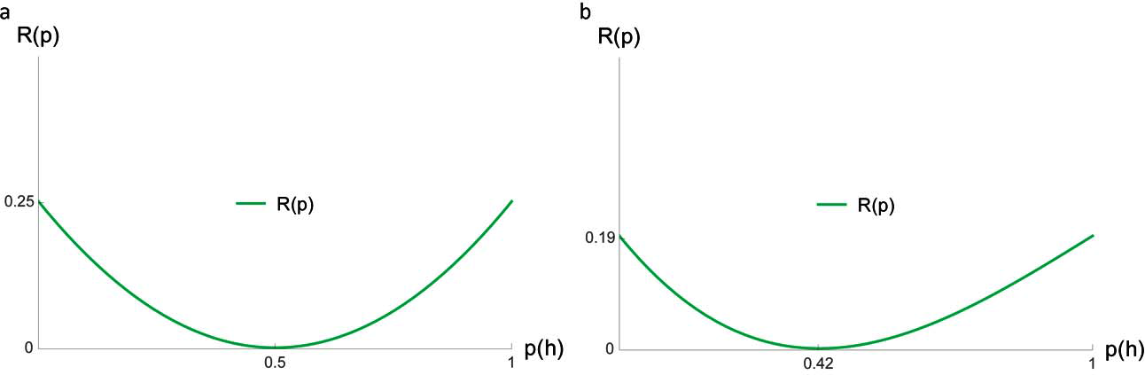
The symmetry of the embedded scoring rule is encoded in the risk function itself. In particular, it is reflected by the location of the risk function’s minimum. As figure 4 shows, a risk function associated with a $0/1$ symmetric score will reach its minimum at $p\left(h\right)=0.5$ (fig. 4a ), whereas if the risk reaches its minimum elsewhere on the unit interval the embedded score must be asymmetric (fig. 4b ).

Figure 4.

Epistemic risk function: a, symmetric risk function; b, asymmetric risk function.

I refer to risk functions such as the one in figure 4a as symmetric: it reaches its minimum at $p\left(h\right)=0.5$, and its shape on [0, 0.5) is a reflection of its shape on (0.5, 1]. Symmetry in the risk function is related to the $0/1$ symmetry of the scoring rule: a scoring rule is $0/1$ symmetric only if its associated risk function is symmetric.

Therefore, we should distinguish at least two different ways of valuing accuracy: a symmetric risk function corresponds to a way of valuing accuracy in which moving away from the truth in either direction is equally bad, whereas an asymmetric risk function implies a way of valuing accuracy in which unit changes in the direction of false positives/negatives get weighted differently at different credal values. Indeed, they may not be weighted equally at any place. It is not enough, therefore, to declare that we should seek truth and avoid error. Such an epistemic norm is underspecified. We need to decide further how to trade-off the potential costs of different types of mistakes. The epistemic risk function is flexible enough to encode different ways of balancing the competing costs.

So far we have exploited only the location of the risk function. But the risk function in figure 4b is not just shifted to the left. Speaking picturesquely, it is also pressed against the y-axis. As a result, there is both a within and between difference in its concavity: it is (a) steeper to the left of its risk-free point than it is to its right, and (b) it is not equally concave as compared to the risk function in figure 4a , whose embedded score is symmetric. These properties add further texture to the proposed measure of risk, reinforcing the idea that risk is a measure of alethic sensitivity to error. To exploit the concavity of the risk function, we need to revisit another quantity.

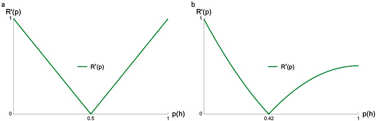
Let $h\left(p\right)=s_1\left(p\right)-s_0\left(p\right)$. For example, when $p=0.8$, h(p) is a measure of the length of the dashed vertical line connecting s ₁ and s ₀ at 0.8 in figure 3. The antiderivative of h(p) is R(p). As a result, our definition of epistemic risk implies that R′(p) is equal in absolute value to h(p). This means that the rate at which risk increases as we move away from the risk-free point reflects the increase, in absolute value, between the agent’s best and worst outcomes. As a result, while the risk function itself reflects the agent’s relative sensitivity to unit increases in inaccuracy in the direction of different types of error, its first derivative reflects, instead, the agent’s local sensitivity to risk as a function of her current credence. It is a measure of marginal increases/decreases in risk. For example, the derivative of the risk associated with the Brier score is $2p-1$. As a result, marginal changes in credence away from the risk-free point lead to a constant increase in risk, as figure 5a shows. If we let ΔFP stand for marginal increases in false positive inaccuracy and ΔFN stand for marginal increases in false negative inaccuracy, then a symmetric risk function (such as the Brier score’s) implies that $\Delta \mathrm{FP}=\Delta \mathrm{FN}$.

Figure 5.

Rate of change in epistemic risk: a, constantly increasing epistemic risk aversion; b, unequally increasing epistemic risk aversion.

By comparison, the derivative of the risk associated with the asymmetric score we have been considering is $-(3/2)p^2+3p-1$ (fig. 5b ). For this score, marginal changes in credence away from the risk-free point in the direction of a false negative error lead to bigger changes in risk relative to marginal changes in credence away from the risk-free point in the direction of a false positive error. The agent applying this particular asymmetric score is more worried about marginal increases in false negative inaccuracy than she is about marginal increases in false positive inaccuracy. For this particular asymmetric risk function, $\Delta \mathrm{FN}>\Delta \mathrm{FP}$. This corresponds to the example described above, where h is so important that rejecting it leads to substantial epistemic opportunity cost.

Moreover, marginal increases in risk taper off as the agent approaches categorical false positive error. This makes sense from a Bayesian perspective of scientific inquiry, since having credence .05 in a true and important proposition is not that different from having credence .01 in the same proposition. In both cases, the agent will likely not pursue the idea further. Meanwhile, given her concern about false negative error, her anxiety in that direction persists, leading to near constant marginal changes in risk across the whole [0, .42) subinterval.

We can see this dimension of the agent’s attitude to risk in the second derivative of the risk function. Gibbard (Reference Gibbard2008, 9) calls R″(p) an indicator of the urgency the believer ascribes to getting credences right, by her lights, in the vicinity of p. For the Brier score, $R^{″}\left(p\right)=2$. No matter where the agent’s credence is on the unit interval, her local sensitivity to being mistaken remains the same. For our asymmetric score, $R^{″}\left(p\right)=3-3p$. This is exactly what we described in the previous paragraph. This is a constantly decreasing function from 0 to 1. The agent’s peak local sensitivity to error occurs at categorical false negative error and slowly tapers off as she approaches false positive error. Given the sensitivity of this particular score to false negatives, that is to be expected because $p\left(h\right)=1$ is where false negatives are eliminated altogether.

One might wonder whether this is a reasonable attitude to false positive error. But this example should not be taken as an endorsement of this particular risk function. Rather, I use it to illustrate the flexibility of the proposed approach to capturing a wide range of attitudes to epistemic risk. The concavity of the risk function resembles in some respects the Arrow/Pratt measure of risk aversion for ordinary economic prospects, where the normalized second derivative reflects an agent’s relative sensitivity to the ordinary risk of monetary loss (Pratt Reference Pratt1964; Arrow Reference Arrow1965, Reference Arrow1971).Footnote ¹²

6. Risk and Generalized Entropy

When equation (1) is uniquely minimized at $b=p$ (i.e., the scoring rule is strictly proper) it may be rewritten as follows:

(2)$\begin{array}{}& E_p\left[s_v\right(p\left)\right]={\mathrm{ps}}_1\left(p\right)+(1-p)s_0\left(p\right)\mathrm{.}\end{array}$

Following Grunwald and Dawid (Reference Grunwald and Dawid2004), I refer to this function, E_b [s_v (p)] in which $b=p$, as H(p), the generalized entropy. Let me explain why, as this will be relevant later. Suppose w(p) is a measure of information conveyed by learning that the event h occurs with probability p. What conditions should w satisfy? This is the question Shannon (Reference Shannon1948) seeks to answer. His famous result is a representation theorem showing that the logarithmic construction $w\left(p\right)=k\log \left(p\right)$ uniquely satisfies several intuitively plausible constraints on a measure of information—namely, that w should be a decreasing, continuous, and additive function of p. By the same token −w(p) measures a lack of information, and Shannon entropy is the expectation of w(p) with $k=\mathrm{-1}$.

In the binary case, Shannon entropy becomes $-[p\log \left(p\right)+\left(1-p\right)\log \left(1-p\right)]$. This is equivalent to the expected inaccuracy of the log score, which is strictly proper. But we can think more generally about an entropy function H associated with other strictly proper scoring rules—the weighted average of a different strictly proper score function of the probability. This is generalized entropy. Generalized entropy is an important building block in epistemic utility theory because Savage (Reference Savage1971) gives us a recipe for deriving strictly proper scores from entropy by showing that every twice differentiable concave entropy function corresponds to a strictly proper scoring rule, as follows:

(3)$\begin{array}{}& s_v\left(p\right)=H\left(p\right)+(v-p)H^{\prime }\left(p\right),\end{array}$

where v is the $0/1$ truth-value for the event in question. This relationship is extremely useful. As long as we start from a twice differentiable H(p) concave on [0, 1], we can derive a continuous, truth-directed, strictly proper score.

The entropy function H is closely related to our measure of epistemic risk, R. For example, for the Brier score, risk is equal to $p^{*}-p(1-p)$, whereas entropy is $p\left(1-p\right)$. This relationship is depicted in figure 6a . Meanwhile, for our asymmetric score risk is $p^{*}-p\left(p-1\right)\left(p-2\right)$, whereas entropy is $p\left(p-1\right)\left(p-2\right)$. We can see this in figure 6b .

Figure 6.

Duality between epistemic risk and entropy; a, symmetric case; b, asymmetric case.

The following theorem establishes that this duality between generalized entropy and epistemic risk holds for all strictly proper scoring rules.

In other words, the sum of risk and entropy is constant: $\mathrm{risk}+\mathrm{entropy}=k$. In general, therefore, entropy is a scaled reflection of epistemic risk around the risk-free point $R\left(p^{*}\right)=k$, as figure 6 suggests. But the risk-free credence is also the maximum entropy credence. Therefore, rearranging the duality equation suggests that epistemic risk may be expressed as a measure of entropic change from the maximum entropy credence to the target credence: $R\left(p\right)=H\left(p^{*}\right)-H\left(p\right)$. We will use this expression below to develop a more general measure of epistemic risk.

Note that since we have defined risk in terms of expected inaccuracy, it follows that for a fixed credal value $p\left(h\right)=k$, the risk associated with k is constant. In other words, given any credence, while it is true that the agent’s accuracy for that credence is a random quantity, because the agent does not know whether h is in fact true or false, the amount of risk the agent assumes is fixed, because it is a function of the distance between those two outcomes. As a result, we cannot evaluate epistemic risk from a different credal point. Therefore, while we may consider accuracy in expectation, on this account we should avoid talking about expected epistemic risk. This will be relevant as we consider the import of epistemic risk to the selection of priors in section 8.

Since epistemic risk is dual to entropy, one might question whether we need to introduce a notion of risk, given the large literature on entropic inference.Footnote ¹³ Rather than speaking in terms of increases in epistemic risk, we could instead describe the same changes in terms of decreases in entropy. Although this is true for strictly proper scoring rules, with the effect that risk and entropy are often coextensive, they are independently motivated. We saw this while developing the notion of epistemic risk in terms of sensitivity to different types of graded error. That is, I am not arguing that the risk-free credence function is risk-free because it maximizes entropy. Rather, it is risk free, as we saw, because it eliminates variability in terms of the epistemic outcome. Strictly proper scoring rules have the feature that these two properties do not come apart. For many other scoring rules, we could eliminate variability without maximizing entropy. In such cases, the duality would not apply, and we could not measure epistemic risk in terms of entropic change.

Therefore, even though risk and entropy are extensionally equivalent for strictly proper scoring rules, thinking in terms of risk minimization is conceptually very different from thinking in terms of entropy maximization. An agent might prefer risk-free credences not because they do not go beyond the evidence, even though that might be true, but because from her perspective they give her the best balance of graded error costs. There is a conceptual difference between thinking in terms of minimizing the amount of information an agents brings into the inference problem (the entropic interpretation) and identifying an appropriate trade-off between different types of potential mistakes (the risk interpretation). As a result, we should not think of one concept being reducible to the other. The duality theorem shows that for many scoring rules, entropy and risk are two different ways of conceptualizing the same underlying epistemic facts.

Indeed, insofar as proponents of entropic methods reference risk, it is assumed that a credence function is risk averse because it maximizes Shannon entropy. Jaynes is the most ardent proponent of this position. For Jaynes, the maximum entropy distribution is the most conservative distribution in the sense that it does not permit us to draw any evidentially unwarranted conclusions because it is “as smooth and spread out as possible” subject to the data (Jaynes Reference Jaynes and Rosenkrantz1963/1983, 186). But consider an entropy function that reaches its maximum at $p\left(h\right)=0.9$. An entropy-maximizing agent with this function would not be conservative at all in Jaynes’s sense. In the absence of any data, she would predict h’s occurrence with high confidence. Therefore, for asymmetric risk functions the least risky distribution will not be maximally uniform.

7. Epistemic Risk: The General Case

So far we have considered credence functions for a single proposition h. Now let the sequence ${\left\{h_i\right\}}_{i=1}^n$ form a partition on sample space S. The risk-free credence function becomes the distribution that solves the equation $s_v\left(p_i\right)=s_w\left(p_j\right)$ for all i, j and indicators of truth-value v, w. Since this expression is unwieldy with many outcomes, we can instead identify this as the point of maximum general entropy. Because entropy is the expected inaccuracy of a strictly proper scoring rule, expressing risk in terms of entropic change enables us to harness helpful properties of expectation.

To make use of these properties, we require a random variable and its cumulative distribution function (cdf). A cdf is just a different way of expressing a probability distribution. Let $X:S\to ℝ$ be a random variable that maps outcomes in the sample space to the real numbers and whose mass/density is given by $f\left(X=x\right)$. For each value of x the cdf, defined as $F(X\le x)={\sum }_{x_i\le x}f\left(x\right)$ (for discrete X) and ${\int }_{-\infty }^{x}f\left(t\right)\mathrm{dt}$ (for continuous X), gives us the probability that X is less than or equal to that value. For example, if the random quantity X represents the numerical outcome of a single toss of a die, then $F\left(X\le 3\right)=1/2$ and $F\left(X\le 4\right)=2/3$.

For our purposes, every outcome may be described in terms of the agent’s inaccuracy if that outcome occurs. Therefore, we can define outcomes in terms of random variables as follows: let X be a random variable that maps outcomes from the sample space to the real numbers, where the real numbers represent inaccuracy given by s. For every valid probability distribution on the sample space, there exists an induced probability distribution on X that is likewise valid. The possible values of the random variable now represent inaccuracy scores. Many scoring rules will take values on a small subinterval of ℝ. For example, under the Brier score all outcomes are mapped to [0, 1]. Changing the underlying scoring rule will rescale the random variable. Therefore, when evaluating credence functions in terms of their epistemic risk, we need to identify a random variable that describes outcomes in terms of some particular measure of inaccuracy. With this in mind, we can define the risk-free cdf as follows.

To simplify, I denote the entropy of cdf P as H(P) instead of H_P (X) (a common abuse of notation, since entropy is a property of the probabilities). As emphasized above, P* is not risk free because it maximizes entropy. Rather, this is the probability assignment that eliminates variability in terms of epistemic outcome, which is how we defined the risk-free credence in the simple case. We can now extend our definition of epistemic risk as follows.

Recall that in the simple case, this definition was motivated as a measure of the “spread” between the agent’s inaccuracy if the proposition is true and her inaccuracy if the proposition is false. It remains to be shown that the general definition given here is motivated by the same underlying conceptual framework.

To see that this is indeed the case, I draw on Rothschild and Stiglitz’s (Reference Rothschild and Stiglitz1970) notion of a mean-preserving spread. Informally, one probability distribution is a mean-preserving spread of another if the second is a transformation of the first obtained by pushing probability mass/density to the tails of the distribution without affecting its expected payoff. In the case of ordinary economic lotteries, distributions are given in terms of wealth. For example, a lottery that pays $0 or $10 with equal probability is a mean-preserving spread of one that pays $6 or $4, or one that guarantees $5.

In the epistemic context, the outcomes of a “lottery” cannot be specified exogenously. Rather, the scale (i.e., scoring rule) is exogenous, but the outcome, given in terms of that scoring rule’s inaccuracy, depends on the probability assignment itself. For example, assuming the Brier score, a credence $p\left(h\right)=0.8$ in a single proposition h is effectively an epistemic lottery that pays ${(1-0.8)}^2=.04$ if h is true and ${(0-0.8)}^2=.64$ if h is false. Now consider a more extreme credence like $p\left(h\right)=0.9$. The latter is a probabilistic spread of the former because it is a transformation accomplished by taking the probability assigned to h and making it even more extreme while at the same time taking the probability assigned to its negation and making it correspondingly more extreme in the opposite direction. Assuming the agent is coherent, there is a quantity that is preserved every time we spread out probability like this, namely, the simple mean given by $1/\left|S\right|$, where |S| is the length of the partition. As long as we keep this quantity fixed, every such spread guarantees an increase in risk. In this sense, a mean-preserving spread of a credence function implies an increase in that credence function’s epistemic risk. By expressing a credence function in terms of its cdf, we can give a general definition of mean-preserving spreads and prove this relationship.

For example, suppose {h ₁, h ₂, h ₃} is a partition on S and we want to measure the epistemic risk of credence function p (or equivalently, its cdf P) given by 〈1/5, 3/5, 1/5〉 under the Brier score.Footnote ¹⁴ Since the Brier score is 0/1 symmetric, we know that its risk-free credence function p* is the uniform 〈1/3, 1/3, 1/3〉.

Before we move on, note that everything we say below will hold for nonsymmetric scoring rules as well. To illustrate, we could use instead a nonsymmetric weighted quadratic score that determines the accuracy assigned to proposition h by ${(v-\mathrm{pr}(h\left)\right)}^2+m/n$, where h is the mth cell in a partition and n is the number of cells. If ordering the cells is not appropriate, we could determine the weights some other way. The important thing is that the weights capture our attitudes to error with respect to each possible outcome. With three propositions again, the risk function of such a score would be minimized with the probabilities 〈.17, .30, .53〉. These are now the (nonuniform) risk-free credences. Notice that the probabilities increase from the first cell to the last. This is to be expected because such a scoring rule penalizes errors with increasing severity as we move up the sequence generating the partition. Because we are most sensitive with respect to errors in the direction of h ₃, that outcome is most sticky, so to speak, and the risk-free credences are extra cautious in its direction.

In any case, to keep things simple, I will continue with the symmetric example. To evaluate the spread of our target credence function from the risk-free credences, we write the cdfs of both credence functions, P and P*, as follows:

$\begin{array}{cccc}{P}^{*}=& \{\begin{array}{cc}0& \text{for }x<{(1/3)}^2\\ 2/3& \text{for }{(1/3)}^2\le x<{(2/3)}^2\\ 1& \text{for }x\ge {(2/3)}^2\end{array}& P=& \{\begin{array}{cc}0& \text{for }x<{(1/5)}^2\\ 4/5& \text{for }{(1/5)}^2\le x<{(4/5)}^2\\ 1& \text{for }x\ge {(4/5)}^2\end{array}\end{array}$

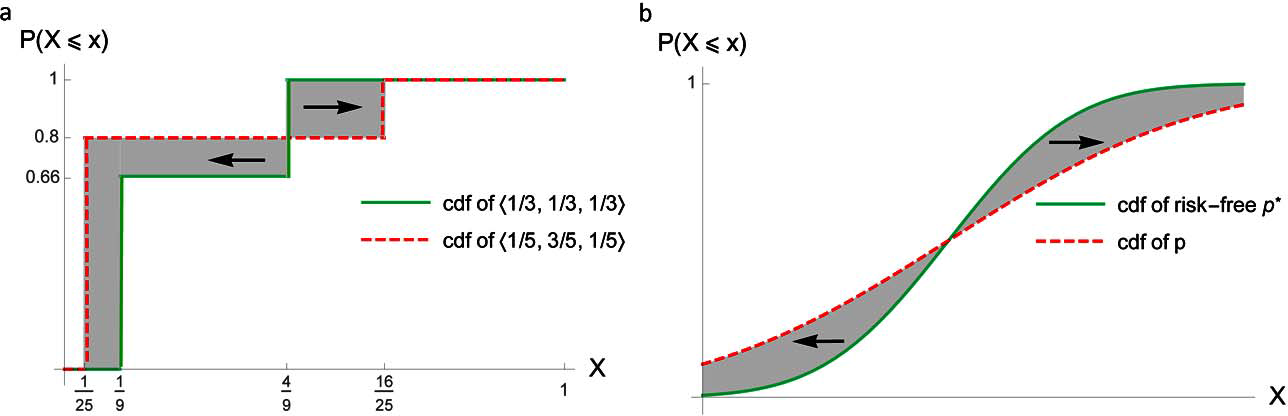
Figure 7a depicts the plot of each cdf. The arrows indicate the spread in probability generated by moving from P* to P. This is harder to visualize for discrete cdfs. To make the idea more intuitive, figure 7b depicts two arbitrary cdfs of a continuous random variable X, where one is a mean-preserving spread of the other.

Figure 7.

Mean-preserving epistemic spreads; a, discrete credence function; b, continuous credence function.

Notice that for any value of X, representing an outcome in terms of inaccuracy, the area underneath the dashed (risky) curve is greater than or equal to the area underneath the solid (safe) curve. Following Rothschild and Stiglitz (Reference Rothschild and Stiglitz1970), we can use this quantity to define mean-preserving epistemic spreads.

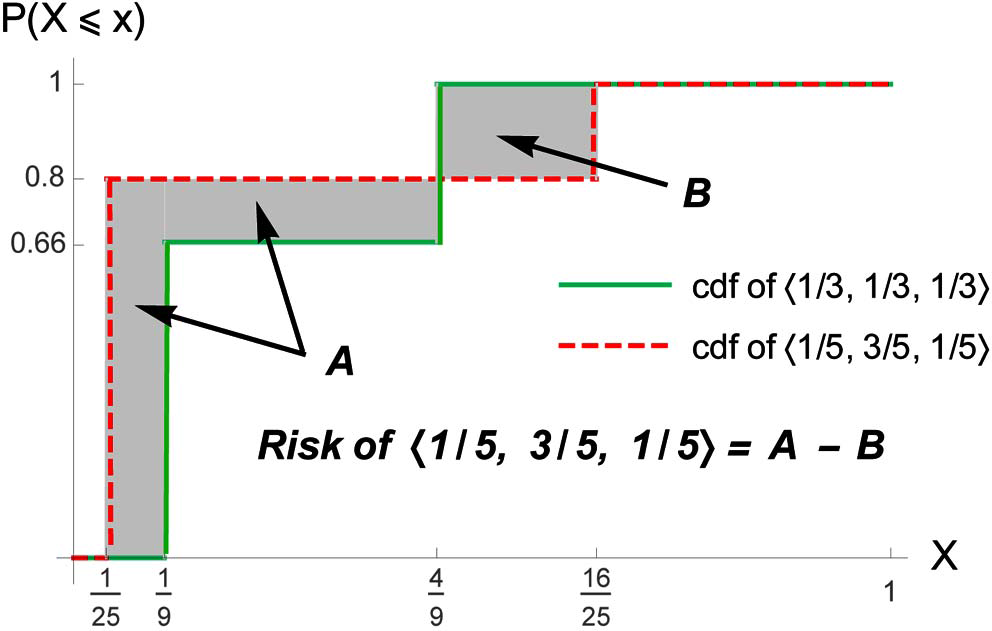
In the single proposition case, this implies that one probability q(h) is a mean-preserving epistemic spread of another probability p(h) if $\left|s_1\right(p)-s_0(p\left)\right|<\left|s_1\right(q)-s_0(q\left)\right|$. This is consistent with our definition of epistemic risk in the simple case as the integral of the absolute difference between s ₁ and s ₀. Therefore, by using mean-preserving epistemic spreads to measure risk, we measure the difference in area underneath the risk-free cdf and the target cdf. In figure 8, this is the difference of the two rectangles labeled A and the rectangle labeled B.

Figure 8.

Epistemic risk as entropic change.

This measure of epistemic risk, in terms of the change in area underneath the cdf, developed by analogy to Rothschild and Stiglitz’s (Reference Rothschild and Stiglitz1970) approach to ordinary risk, preserves the motivation given for measuring epistemic risk in the simple case as sensitivity to approaching different types of error. In the general case, however, epistemic risk reflects an agent’s sensitivity to graded inaccuracy with respect to any given outcome in the sample space. As a result, we no longer have type I and type II errors only. Instead, we have n error types for $\left|S\right|=n$ possible outcomes.

We are now in a position to show that our definition of epistemic risk in terms of entropic change corresponds to the general interpretation of epistemic risk given in terms of mean-preserving epistemic spreads. For any given cdf P, as the area underneath it, given by ${\sum }_{i=1}^{n}P\left(x_i\right)$ (for discrete X) or ${\int }_{X}P\left(x\right)\mathrm{dx}$ (for continuous X), decreases, the quantity $1-{\sum }_{i=1}^{n}P\left(x_i\right)$ (for discrete X) or $1-{\int }_{X}P\left(x\right)\mathrm{dx}$ (for continuous X), increases. In figure 8, for example, for each cdf, this is the area to its left and bounded above by the line $P\left(X\le x\right)=1$. This quantity is equal to the expectation of X. This relationship is a consequence of Fubini’s Theorem. Importantly for us, since X maps outcomes to inaccuracy scores, the expectation of a random variable X with cdf P is precisely the entropy of P, H(P), provided the underlying inaccuracy scale given by s is strictly proper. Furthermore, on any given sample space S, the risk-free cdf will be the cdf that has the smallest area underneath it. Equivalently, it will be the cdf that has the largest area to its left. We can see this in figure 8. In more familiar words, the risk-free credence is the maximum entropy credence. Again, however, it is risk free not because it maximizes entropy but rather because this is the point where the agent’s sensitivity to graded error in the direction of every possible outcome in the sample space is equal. And again it turns out, as in the simple case, that for strictly proper scores this is also the point that maximizes entropy. Therefore, as measured in terms of mean-preserving epistemic spreads, risk may be given as the difference between the entropy of the risk-free cdf and the target cdf. This is precisely the quantity A–B in figure 8, and it corresponds exactly to how we have defined epistemic risk, as $H\left(P^{*}\right)-H\left(P\right)$.

For example, consider the cdfs depicted in figure 8. To measure the risk of P, we first determine the entropy of the risk-free P*. The area to the left of its cdf is a sum of two rectangles: one of length 1/3 and width 2(1/3) and another of length 2(1/3) and width 1/3. This is 4/9. Next, we determine the entropy of P. Following the same approach, we get 8/25. Since risk is given in terms of entropic change, the risk of P is $4/9-8/25=.12$. This leads to the following theorem.

As a result, every mean-preserving epistemic spread increases variability in the underlying outcomes, increases risk, and (if s is strictly proper) decreases entropy.

Since the approach we have developed requires identifying an inaccuracy scale before evaluating the risk of a credence function, one might reasonably wonder how general the risk ordering of credence functions will be. For example, suppose we have the same two credence functions as in the previous paragraph, $p^{*}=〈1/3,1/3,1/3〉$ and $p=〈1/5,3/5,1/5〉$, but we define epistemic outcomes logarithmically instead of quadratically. That is, the x-axis now measures inaccuracy in terms of the log score. The y-axis still measures cumulative probability. Would it still be the case that $R\left(P\right)>R\left(P^{*}\right)$? If so, would the risk order be preserved for any arbitrarily chosen set of cdfs?

For most families of scoring rules considered in the literature, including some improper scores, the risk ranking of credence functions will be consistent. This includes the Brier, log, spherical, and absolute value scores. But it does not include the asymmetric score we have been considering throughout. This is because the asymmetric score has a different risk-free point, and risk is measured in terms of deviation from that risk-free point. Of course, if we take two asymmetric scores with the same risk-free point, wherever it happens to be, then it is very likely that the risk ordering between them will be consistent. Specifically, for any two scoring rules, if they share the same risk-free point, and their risk function is convex, then the risk order of credence functions between them will be consistent. The following theorem captures this relationship.

This result expands the reach of our approach to epistemic risk to the vast majority of commonly considered families of scoring rules.

That is not to say, however, that all information encoded in the risk function will be preserved across different scoring rule transformations of it. Consider the Brier and log risk functions. While they are both convex and share the same risk-free point, their derivatives are different. As a result, while a Brier-to-log transformation preserves an agent’s risk ordering, it does not preserve her attitudes to unit changes in inaccuracy nor does it preserve her local sensitivity to marginal changes in risk. We could have two agents who rank two prospective credence functions equally in terms of risk, yet while one agent finds that degree of risk tolerable, the other considers it to be inappropriate, because of differences in the way they evaluate the potential cost of increasing graded inaccuracy in the direction of any given outcome. This is to be expected, however. We would not want a risk function that erases well-known differences between these scores. As Selten (Reference Selten1998) emphasizes, the log score is hypersensitive in the sense that one’s inaccuracy goes to infinity as the probability assignment goes to 0 or 1. This hypersensitivity is reflected in the curvature of its associated risk function.

Before we move on, it is worth pausing to clarify the relationship between measures of epistemic risk and measures of attitudes to it. In ordinary economic theory, mean-preserving spreads are used to generate a partial ordering of stochastic alternatives in terms of their degree of risk. Meanwhile, the curvature of an agent’s utility function reflects her sensitivity to risk. Rothschild and Stiglitz (Reference Rothschild and Stiglitz1970) are so influential because they show that risk-averse agents prefer less risky lotteries to more risky ones, as we would expect. In the epistemic case, we have a similar relationship, to an extent. The epistemic risk function enables us to rank prospective credence functions in terms of their risk. Meanwhile, an agent is risk averse if her scoring rule is convex. And in the absence of information, an agent with a convex scoring rule would prefer a less risky credence function to a more risky one.

Risk increases with mean-preserving spreads in accuracy, and all truth-directed scoring rules with the same risk-free point agree on this ranking, regardless of their convexity. But the way risk is judged by agents to increase—the rate and acceleration of the increase in risk—reflects the agents’ attitudes to risk. Such attitudes originate in the curvature of their scoring rule (i.e., the way they value accuracy). As a result, the risk ranking of credence functions in epistemology is not completely independent from the agents’ attitudes to risk in the way that stochastic dominance is independent of a utility measure. This is inescapable, however. In economic theory, the probabilities and outcomes are both exogenously specified (e.g., the monetary prizes are determined in advance and their associated probabilities given by a roulette wheel), whereas in epistemology the accuracy outcomes are a function, in part, of the way probabilities are distributed. In other words, in the epistemic case one’s payoff is directly determined by the probability one assigns to that outcome. By contrast to economic lotteries, we do not have probabilities for the outcomes that are specified from the outside and independent of the “money” (i.e., probability) wagered on them.

8. Risk, Priors, and the Principle of Indifference

By developing a theory of accuracy dominance Joyce (Reference Joyce1998, Reference Joyce, Huber and Shmidt-Petri2009) gives us a powerful tool for evaluating the quality of an agent’s beliefs. The theory of epistemic risk enables us to go further in terms of our understanding of the normative dimensions of an agent’s credal state. One might ask how these attitudes to risk will manifest themselves. Nearly everyone in the literature agrees that an agent should choose the credence function that, in light of her evidence, minimizes her expected inaccuracy. As a result, attitudes to risk are not going to play a direct role in one’s choice (fictional or otherwise) of what to believe. But this is not the role of risk in ordinary expected utility theory either. We do not consult our sensitivity to risk in order to make a choice. Instead, our choice reflects our attitudes to risk. Roughly the same is true in the epistemic case.

However, risk attitudes can play a more direct role at the beginning of one’s epistemic practices: in particular, agents’ attitudes to risk (i.e., how much of it they are willing to assume) together with the shape of their risk function (e.g., symmetric, nonsymmetric) can motivate a choice of prior in the absence of information. The Laplacean POI is often given as a crude guide for this task. In the absence of information to privilege one outcome over others given a partition of the sample space, one should assign equal probability to each. It is assumed, therefore, that given an appropriate partition the POI recommends uniform credences. The most well-known problems with this principle stem from its association with uniformity. In particular, the uniform distribution over one partition may be logically inconsistent with the uniform distribution over a simple transformation of that partition.Footnote ¹⁵ Epistemic risk provides a new perspective on the POI—one that enables us to dissociate it from uniformity.

If we have an agent whose risk function is convex and symmetric, then the credence function that obtains minimum epistemic risk will be uniform. This is because a symmetric and convex epistemic risk function is associated with a 0/1 symmetric scoring rule. The proof of this is trivial. Under such a score, an agent would be indifferent between taking a bet whose payoffs are given in terms of inaccuracy on any proposition when the probabilities assigned to them are equal. Therefore, minimizing epistemic risk under these conditions suggests the same credence function as the ordinary Laplacean POI. As a result, we can think about the Laplacean POI as a heuristic for identifying the risk-minimizing credences under a very particular class of risk functions. However, it is only in the special case of convex and symmetric risk functions that indifference and uniformity are guaranteed to coincide.

This line of thought enables us to go further. We can consider risk-minimizing heuristics for risk functions that do not satisfy these conditions. For such risk functions, the credences that obtain minimum risk will be such that the agent is indifferent with respect to taking a bet on any outcome, but they will not be uniform. Therefore, we may think of each risk function as having its own associated POI, but when convexity and symmetry are not satisfied it is not guaranteed to be Laplacean. By recasting the Laplacean POI as a risk minimization principle, we can identify the normative commitment presupposed in its endorsement. In particular, it requires the agent to care equally about approaching different types of error. Just as importantly, we can sever its association with uniformity. For scoring rules that are not 0/1 symmetric, there will be a credence function in which the agent is indifferent regarding the outcomes, but it will not be uniform.Footnote ¹⁶

To illustrate the relationship between epistemic risk and indifference principles, suppose we have two agents, A and B, whose risk functions, given a simple partition involving h and its negation, are given by the symmetric and asymmetric risk functions we have been considering, as follows:

$\begin{array}{cc}{r}_A\left(p\right)=p^{*}-p(1-p)& r_B\left(p\right)=p^{*}-p(p-1)(p-2)\end{array}$

These functions are depicted in figures 4a and 4b , respectively. A’s epistemic risk function is associated with the ordinary Brier score. Therefore, if A seeks to minimize epistemic risk in the absence of information his credence function will be (0.5, 0.5). Under these conditions, minimizing epistemic risk and applying the ordinary Laplacean POI give the same recommendation. Now consider B. Given her risk function, the risk-free credences are (.42, .58). Given these credences, B would be indifferent between taking a bet on h or its negation. But this credence function is not uniform. In other words, (.42, .58) is the prior credence function recommended by a non-Laplacean indifference principle associated with B’s nonsymmetric epistemic risk function.Footnote ¹⁷

Pettigrew (Reference Pettigrew2016a) argues for the Laplacean POI from considerations of accuracy, as measured by the Brier score, and a minimax decision rule. On the approach we have developed, a more general result follows: the requirement to identify the prior that minimizes epistemic risk under a convex and symmetric risk function will always suggest the same credence function as the ordinary Laplacean POI. But this is not an argument for the uniform prior. Rather, it suggests that we have a family of indifference principles associated with different epistemic risk functions. And whether an agent finds the Laplacean POI attractive depends on her normative judgments regarding the relative severity of approaching different types of graded error.

The notion, due especially to Jaynes (Reference Jaynes1957), that the right prior is to be found by identifying the maximum entropy distribution is a combination of two separate normative principles: (a) that one ought to minimize epistemic risk and (b) that one ought to evaluate epistemic risk using a convex, symmetric function. The framework developed here enables us to distinguish the two principles: even if we agree that minimizing epistemic risk is desirable, the appropriate prior may not be uniform. Therefore, the Jaynesian commitment to maximum entropy priors is a commitment to a particular attitude to how much risk is rationally permissible (as little as possible) and how different types of errors are to be evaluated (equally). These are strong normative assumptions that, despite the size of the literature on the problem of the priors and the principle of maximum entropy, had not been adequately addressed.