


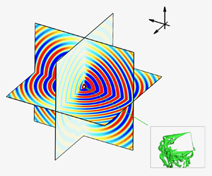



1. Introduction
The aeroacoustics generated by flapping wings is ubiquitous in aerial animal flight. Wing-flapping-generated sound (Clark Reference Clark2021) is essential in courtship (Spieth Reference Spieth1974; Gibson & Russell Reference Gibson and Russell2006) and sexual recognition (Warren, Gibson & Russell Reference Warren, Gibson and Russell2009) for many insects. Some insects, such as Drosophila melanogaster, can respond to sounds that share similar frequency characteristics to their own species (Robert & Göpfert Reference Robert and Göpfert2002). Apart from biological systems, aeroacoustics generated by flapping wings is of importance in micro aerial vehicles (MAVs), especially in applications like military reconnaissance and environmental monitoring where quiet operation is crucial, because applications of flapping wings (Platzer et al. Reference Platzer, Jones, Young and Lai2008; Shyy et al. Reference Shyy, Aono, Chimakurthi, Trizila, Kang, Cesnik and Liu2010; Ravi et al. Reference Ravi, Kolomenskiy, Engels, Schneider, Wang, Sesterhenn and Liu2016) in the MAVs (Young & Garratt Reference Young and Garratt2020; Chen et al. Reference Chen, Cheng, Zhou, Zhang and Wu2024) have been growing due to their high-lift performance.
In order to explain the aeroacoustics generated by flapping wings, it is necessary to introduce their force generation and the associated mechanisms, of which the majority are about the vortical structures. Early efforts on flapping wings were focused on their force generation (Ellington Reference Ellington1984; Platzer et al. Reference Platzer, Jones, Young and Lai2008; Shyy et al. Reference Shyy, Aono, Chimakurthi, Trizila, Kang, Cesnik and Liu2010). In particular, the influences of parameters (such as kinematics, aspect ratio and Reynolds numbers) on forces have been investigated. The kinematics of simplified flapping motions on the force generation have been extensively studied, including plunging and pitching motions in forward flight (Lai & Platzer Reference Lai and Platzer1999; Young & Lai Reference Young and Lai2007; Visbal Reference Visbal2009; Kim & Gharib Reference Kim and Gharib2010), and translating/stroke and pitching motions in hovering flight (Birch & Dickinson Reference Birch and Dickinson2001; Poelma, Dickson & Dickinson Reference Poelma, Dickson and Dickinson2006; Garmann, Visbal & Orkwis Reference Garmann, Visbal and Orkwis2013; Medina & Jones Reference Medina and Jones2016). It is found that unsteady flows over the flapping wing generate vortices near the wing edges which play an important role in the force generation in addition to the added mass (Chang Reference Chang1992; Sane & Dickinson Reference Sane and Dickinson2001). These vortical structures are demonstrated in figure 1, including leading-edge vortex (LEV) (Ellington et al. Reference Ellington, Van Den Berg, Willmott and Thomas1996; Ford & Babinsky Reference Ford and Babinsky2013; Eldredge & Jones Reference Eldredge and Jones2019), trailing-edge vortex (TEV) (Shyy et al. Reference Shyy, Aono, Chimakurthi, Trizila, Kang, Cesnik and Liu2010; Han et al. Reference Han, Chang, Kim and Han2015), tip vortex (TV) (Ringuette, Milano & Gharib Reference Ringuette, Milano and Gharib2007; Shyy et al. Reference Shyy, Trizila, Kang and Aono2009; Kim & Gharib Reference Kim and Gharib2010), root vortex (RV) (Shyy et al. Reference Shyy, Aono, Chimakurthi, Trizila, Kang, Cesnik and Liu2010) and sometimes secondary vortex (SV) (Lu, Shen & Lai Reference Lu, Shen and Lai2006). The LEV is the most prominent flow structure. It creates a low-pressure zone above the wing, responsible for most of the lift generation during the translation/middle stroke phase (Ellington et al. Reference Ellington, Van Den Berg, Willmott and Thomas1996; Liu et al. Reference Liu, Ellington, Kawachi, Van Den Berg and Willmott1998). Garmann & Visbal (Reference Garmann and Visbal2014) found that the aerodynamic force coefficients of revolving wings are hardly changed when the aspect ratio is larger than 2, as the chordwise evolution of LEV at outboard region is limited by the trailing edge, leading to the loss of the negative pressure above the wing. Jones & Babinsky (Reference Jones and Babinsky2011) investigated a waving wing at different Reynolds numbers, finding that the LEV sheds earlier at lower Reynolds numbers, leading to the earlier disappearance of the low-pressure zone and consequently a reduction of the aerodynamic forces. Other vortices contribute to the force in a similar way, i.e. through creating a low-pressure zone. Their contributions to the force are affected by shapes, kinematics and material properties of the wing (see e.g. Tian et al. Reference Tian, Luo, Song and Lu2013; Shahzad et al. Reference Shahzad, Tian, Young and Lai2016; Huang et al. Reference Huang, Bhat, Yeo, Young, Lai, Tian and Ravi2023). Therefore, their evolution and interaction are quite diverse, creating complexities in studying flapping wings. For example, the interaction between LEV and the boundary layer could generate an SV which influences the force generation (Lu et al. Reference Lu, Shen and Lai2006). Overall, the variations of these parameters will lead to the change of the vortex dynamics around the flapping wing, and thus modify the aerodynamic forces which could ultimately affect the aeroacoustics generated by the wings.
Vortical structures around a flapping wing: LEV, TEV, TV, RV and SV.

Conservation of momentum and force partition methods can be used to uncover the relationship between the vorticity and forces (Wu, Ma & Zhou Reference Wu, Ma and Zhou2007). Wu (Reference Wu1981) proposed the vorticity moment theory based on the conservation of momentum, connecting the aerodynamic force of a body moving in a fluid to the time derivative of the total first moment of the vorticity field in an open space. Based on a derivative of moment transformations, Wu, Pan & Lu (Reference Wu, Pan and Lu2005) further proposed two formulae to account for the aerodynamic forces on an arbitrary body in the form of control surface integral including the viscous vortical effects. This method was later successfully adopted by Li & Lu (Reference Li and Lu2012) to calculate the aerodynamic forces of flapping plates by considering the ring-like vortical structures in the wake, finding that the force on a flapping plate is dominated by the flow structures close to the plate. A force and moment partitioning method is a powerful tool for analysing complex vortex flows through delineating the contribution of vortex-induced effects (Wu et al. Reference Wu, Ma and Zhou2007; Menon, Kumar & Mittal Reference Menon, Kumar and Mittal2022). For example, Seo, Menon & Mittal (Reference Seo, Menon and Mittal2022) proposed a force partitioning method for studying the vortex evolution on the surface pressure fluctuation and acoustics of a two-dimensional (2-D) flapping foil. Further discussion on the relationship between vortices and aerodynamic forces can be found in Wu, Liu & Liu (Reference Wu, Liu and Liu2018). As the vortex flows dominate in flapping wings, their forces can be estimated by considering the time derivative of the vortex impulse, which is the basis of scaling laws for the aerodynamic forces of flapping wings (see e.g. Dewey et al. Reference Dewey, Boschitsch, Moored, Stone and Smits2013; Kang & Shyy Reference Kang and Shyy2013; Lee, Choi & Kim Reference Lee, Choi and Kim2015; Ehrenstein Reference Ehrenstein2019; Liu, Liu & Huang Reference Liu, Liu and Huang2022). In these scaling laws, the flapping frequency with its intrinsic connection with vortices’ evolution period is considered as an important factor for scaling the aerodynamic forces.
The aerodynamic forces acting on a moving body, which are determined by the vortex flows, have strong effects on the acoustics (Seo, Hedrick & Mittal Reference Seo, Hedrick and Mittal2019; Tian Reference Tian2020). Therefore, the vortical flows as well as their evolution would have a strong impact on the acoustics. However, the aeroacoustic characteristics have received less attention compared with the aerodynamics and vortical flows of flapping wings but have attracted growing effort recently. The aeroacoustics of flapping wings have been investigated experimentally (see e.g. Sueur, Tuck & Robert Reference Sueur, Tuck and Robert2005; Arthur et al. Reference Arthur, Emr, Wyttenbach and Hoy2014; Zhou et al. Reference Zhou, Sun, Fattah, Zhang and Huang2019) and numerically (see e.g. Nagarajan & Lele Reference Nagarajan and Lele2005; Nagarajan, Hahn & Lele Reference Nagarajan, Hahn and Lele2006; Bae & Moon Reference Bae and Moon2008; Inada et al. Reference Inada, Aono, Liu and Aoyama2009; Wang & Tian Reference Wang and Tian2020). The noise generated by a flyer in forward and aft directions is dominated by the first harmonic (flapping frequency,  $f_o$) while the noise at the sides is dominated by the second harmonic (
 $2f_o$) (Sueur et al. Reference Sueur, Tuck and Robert2005; Arthur et al. Reference Arthur, Emr, Wyttenbach and Hoy2014). This is because that the wing creates one-periodic thrust in the forward and aft directions, and two-cycle lateral forces in side directions during one flapping cycle. Vorticity features also have an impact on acoustics. For example, the vortex shedding frequency near the trailing edge of a pitching NACA0012 aerofoil at high Reynolds numbers corresponds to the central frequency of the noise hump in the spectrum (Zhou et al. Reference Zhou, Sun, Fattah, Zhang and Huang2019). For a 2-D elliptical wing undergoing hovering and forward flights, a dipole source of flapping frequency is generated from the transverse motion and higher-frequency dipole sources arise from trailing edge scattering during tangential motion (Bae & Moon Reference Bae and Moon2008). The dipole sources are generated by the pressure difference between the two sides of the wings (Inada et al. Reference Inada, Aono, Liu and Aoyama2009). A more detailed study (Seo et al. Reference Seo, Hedrick and Mittal2019) showed that the time derivative of the surface pressure is the most important noise source for the aeroacoustics of flapping wings at low Mach numbers (also see Tian Reference Tian2020; Clark Reference Clark2021). Flexibility of wings could enhance the mean force production and reduce the noise (Geng et al. Reference Geng, Xue, Zheng, Liu, Ren and Dong2017).
As noted above, the aerodynamic force fluctuations are correlated with the surface pressure variation caused by vortical structure evolution, hence new insights into the mechanism of aeroacoustics generation could be obtained by investigating the vortical structure evolution. Nedunchezian, Kang & Aono (Reference Nedunchezian, Kang and Aono2019) found that the kinematics of the wing play an important role in determining the noise level and that the variations of the vortical structures’ topology may account for the difference in noise level. Clark (Reference Clark2021) discussed the vortex–wing interaction and acknowledged that the noise generated by vortices can be promoted if the vortices are in the vicinity of a wing (also noted by Curle (Reference Curle1955)). By using a force partitioning method, Seo et al. (Reference Seo, Menon and Mittal2022) investigated the influences of each vortical structure and kinematic parameters on the aeroacoustics of a 2-D pitching NACA0015 aerofoil finding that the LEV plays an important role in determining the wing surface pressure and thus the far-field acoustics. However, the influence of characteristic vortices on surface pressure fluctuations in the three-dimensional (3-D) case can be evaluated in a more straightforward way without employing the projection method (Seo et al. Reference Seo, Menon and Mittal2022). In addition, it remains unclear which characteristic vortex is dominant in affecting the surface pressure fluctuations in the 3-D case.
To gain insights into the flow and acoustic fields associated with flapping wings, computational fluid dynamics (CFD) is an attractive method. There are two types of CFD methods used for aeroacoustic studies: (i) direct numerical simulation (DNS) and (ii) hybrid methods. In DNS, the compressible Navier–Stokes (NS) equations are solved by high-resolution numerical schemes in which all fluid scales and sound waves are resolved (Colonius, Lele & Moin Reference Colonius, Lele and Moin1997; Sandberg et al. Reference Sandberg, Jones, Sandham and Joseph2009). Direct numerical simulation has been successfully used to investigate the aeroacoustics of flapping wings (Wang & Tian Reference Wang and Tian2019; Wang, Tian & Lai Reference Wang, Tian and Lai2020). Despite its successful applications, the large computational cost has hindered DNS usage, especially for low Mach number flows ( $M<0.1$) where the size of the time step may be restricted more by the time scale of acoustic wave propagation than by that of hydrodynamics. To address these challenges, hybrid methods (Hardin & Pope Reference Hardin and Pope1994; Lele Reference Lele1997; Colonius & Lele Reference Colonius and Lele2004) have emerged as a promising approach. In these methods, the hydrodynamic field is acquired through direct solutions of the compressible or incompressible NS equations. Concurrently, the acoustic field is evaluated using simplified models (e.g. linearised Euler equations (Bailly & Juve Reference Bailly and Juve2000) and Green's function coupling with acoustic analogy (Lyrintzis Reference Lyrintzis2003; Farassat Reference Farassat2007)). The hybrid methods (e.g. coupling the incompressible simulation with the acoustic analogy) could relax the time step restriction and the grid requirement for resolving the acoustic wave propagation in the DNS at low Mach number flows. Therefore, a hybrid method coupling an incompressible solver and Farassat formulation 1A is used in this work.
This work is to develop a connection between the pressure fluctuation and the vortex evolution for a 3-D hovering wing where rotational motions are involved, and a simple scaling law for noise source. The dominant vortex on the time derivative of the surface pressure and its evolution will be addressed. To achieve this, a zero-thickness low-aspect-ratio ( $AR=1.5$) rectangular hovering wing at a Reynolds number of 1000 and a Mach number of 0.04 is numerically investigated by solving the incompressible NS equations with the diffused interface immersed boundary (IB) method. By using the wing model, the Farassat formulation 1A is first validated. A simplified acoustic model based on the Ffowcs Williams-Hawkings (FW-H) acoustic analogy is expressed in the frequency domain and validated against the Farassat formulation 1A. Furthermore, the variation of the surface pressure is analysed and the numerical results are incorporated to illustrate the underlying relationship between the surface pressure variation and vortices evolution. Finally, a scaling analysis of the vortex acoustic source is conducted.
This paper is organised as follows. The physical model and numerical method are described in § 2 with validations, mesh and computational domain convergence studies presented in the Appendix (A). The numerical results are presented and discussed in § 3, and concluding remarks are provided in § 4.
2. Physical model and numerical method
2.1. Physical model
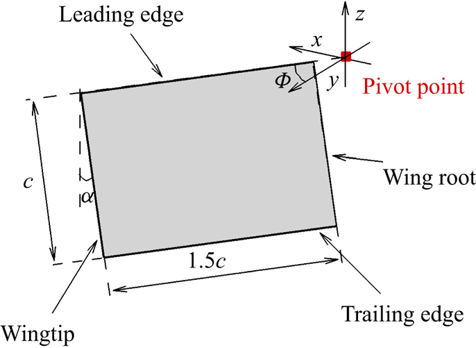
As shown in figure 2, a zero-thickness rectangular wing with a chord length of  $c$, and a wingspan of
 $1.5c$, is considered. A low aspect ratio (
 $AR=1.5$) is used due to its high power economy and low computational cost (Shahzad et al. Reference Shahzad, Tian, Young and Lai2016). The pivot point is 0.1c away from the wing root. For hovering flight, insect wings typically have three degrees of freedom (Ellington Reference Ellington1984). Here, we assume the wing undergoing stroke rotation around the
 $z$-axis and pitching motion around the leading edge. The stroke plane deviation is usually very small (Chen et al. Reference Chen, Gravish, Desbiens, Malka and Wood2016; Shahzad et al. Reference Shahzad, Tian, Young and Lai2018), and thus ignored here. The stroke and pitching motions, akin to those described in Dai, Luo & Doyle (Reference Dai, Luo and Doyle2012), are adopted,
 \begin{equation} \varPhi(t)=\frac{\rm \pi}{5}\sin\left(2{\rm \pi} f_ot+\frac{\rm \pi}{2}\right), \quad \alpha(t)=\frac{\rm \pi}{6}\sin(2{\rm \pi} f_ot), \end{equation}
where  $\varPhi$ is the angle between the leading edge and the
 $y$-axis,
 $\alpha$ is the angle between the chord line and the
 $z$-axis,
 $f_o = 0.25$ is the flapping frequency and
 $t$ is the time (
 $f_o$ and
 $t$ are normalised by
 $U_{ref}$ and
 $c$). Note that a small stroke angle is used to reduce the computational cost. According to the scaling laws and previous studies (see e.g. Lee et al. Reference Lee, Choi and Kim2015; Wang & Tian Reference Wang and Tian2020), this choice is sufficient to achieve the objective of this work.
The schematic shows dimensions and definitions of the stroke angle ( $\varPhi$) and the pitching angle (
 $\alpha$) for a zero-thickness 3-D rectangular flapping wing.
Here, a Reynolds number ( $Re=U_{ref}c/\nu$) of 1000 and a Mach number (
 $M=U_{ref}/c_o$) of 0.04 are chosen, where
 $U_{ref}$ is the mean tip velocity and defined as
 $4{\rm \pi} /5 f_o (AR+0.1)c \approx 4cf_o$,
 $\nu$ is the kinematic viscosity and
 $c_o$ is the sound speed. The chosen Reynolds number and the Mach number fall in the range of some insects (Eldredge & Jones Reference Eldredge and Jones2019; Hightower et al. Reference Hightower, Wijnings, Scholte, Ingersoll, Chin, Nguyen, Shorr and Lentink2020) and allow us to investigate the characteristic features of both flow and acoustic fields at a relatively low computational cost.
2.2. Numerical methods
Here the incompressible NS equations solver and the FW-H acoustic analogy are used. A simplified model based on the far-field approximation and the FW-H acoustic analogy is proposed here.
2.2.1. Fluid solver
As the operation speed for bio-inspired flapping wings is low (Hightower et al. Reference Hightower, Wijnings, Scholte, Ingersoll, Chin, Nguyen, Shorr and Lentink2020), the Mach number is much less than 1. Therefore, the fluid dynamics is governed by the dimensionless 3-D incompressible NS equations,
 $$\begin{gather} \boldsymbol{\nabla}\boldsymbol{\cdot} {\boldsymbol u}=0, \end{gather}$$
 $$\begin{gather}\frac{\partial {\boldsymbol u}}{\partial t} + {\boldsymbol u}\boldsymbol{\cdot}\boldsymbol{\nabla} {\boldsymbol u} ={-} \boldsymbol{\nabla} p +\frac{1}{Re}\nabla^2 {\boldsymbol u} + {\boldsymbol f}, \end{gather}$$
where  ${\boldsymbol u}$ is the fluid velocity,
 $p$ is the pressure and
 ${\boldsymbol f}$ is the body force. Based on previous studies (Jones & Babinsky Reference Jones and Babinsky2010; Garmann et al. Reference Garmann, Visbal and Orkwis2013; Eldredge & Jones Reference Eldredge and Jones2019), the flow fields for flapping wings at a Reynolds number of 1000 are laminar. To verify that the flow is laminar at
 $Re=1000$, our results of including the dynamic Smagorinsky (DS) model (Germano et al. Reference Germano, Piomelli, Moin and Cabot1991) as the subgrid model (Smagorinsky constant
 $C_s$ is chosen as 0.1), not shown here, show insignificant differences (less than 1 %) in the aerodynamic force coefficients from our current simulation without the DS model.
The second-order central difference is used for the spatial derivative while the second-order Crank–Nicolson method is used for time marching. The incompressible NS equations are solved by a projection method consisting of three steps: (i) the momentum equations are solved by a Jacobian-free Newton-Krylov method to obtain the intermediate velocity; (ii) the pressure is updated by solving a Poisson equation with the generalised minimal residual method where the algebraic multigrid method is used as a preconditioner; and (iii) the velocity for the current step is updated based on the solutions of the Poisson equation and the intermediate velocity. More details can be found in Calderer et al. (Reference Calderer, Yang, Angelidis, Khosronejad, Le, Kang, Gilmanov, Ge and Borazjani2015).
The IB method (Peskin Reference Peskin1972; Mittal & Iaccarino Reference Mittal and Iaccarino2005; Huang & Tian Reference Huang and Tian2019) is used to handle the boundary condition on the wing surface. Compared with the arbitrary Lagrangian–Eulerian method (Hirt, Amsden & Cook Reference Hirt, Amsden and Cook1974; Farhat & Lakshminarayan Reference Farhat and Lakshminarayan2014), the fluid grid in the IB method does not have to conform to the geometry of the solid surface or be regenerated if moving boundaries are involved. Thus, the IB method is more efficient in coping with moving boundary problems, as considered here. The flow field is discretised with non-uniform Cartesian grids, and the solid surface is discretised by triangle grids. The diffused interface IB method (Peskin Reference Peskin1972; Goldstein, Handler & Sirovich Reference Goldstein, Handler and Sirovich1993; Peskin Reference Peskin2002; Huang & Tian Reference Huang and Tian2019), which is easy to implement and can provide reliable solutions (Huang & Tian Reference Huang and Tian2019; Huang et al. Reference Huang, Liu, Wang, Ravi, Young, Lai and Tian2022), is used to implement the boundary condition at the fluid–structure interface. More details of this method can be found in Ji et al. (Reference Ji, Wang, Ravi, Tian, Young and Lai2022, Reference Ji, Wang, Ravi, Young, Lai and Tian2024).
Here a computational domain with the dimensions  $-5c \le x \le 5c$,
 $-5c \le y \le 5c$ and
 $-5c \le z \le 5c$, is used. A fine grid region (
 $2c \times 1.7c \times 1.2c$) is discretised by uniform fine grids with its size denoted as
 $\varDelta _{min}$ while an outer grid region is discretised by non-uniform grids. Far-field boundary conditions are enforced at the outer boundaries while the diffused interface IB method is incorporated to achieve the no-slip boundary condition at the wing surface. The fluid solver was validated in the previous works (Ji et al. Reference Ji, Wang, Ravi, Tian, Young and Lai2022, Reference Ji, Wang, Ravi, Young, Lai and Tian2024). Convergence studies of the grid and computational domain have been conducted with details presented in the Appendix (A). Based on the convergence studies,
 $\varDelta _{min}=0.01c$ and a computational domain of
 $10c \times 10c \times 10c$ are used for all simulations in this work.
2.2.2. Acoustic solver
To consider the sound generated by a moving boundary, Ffowcs Williams & Hawkings (Reference Ffowcs Williams and Hawkings1969) used the generalised function and rewrote the Curle equation (Curle Reference Curle1955) into the FW-H equation,
 \begin{equation} \left(\frac{1}{c^2_o}\frac{\partial ^2 }{\partial t^2} - \nabla^2 \right)p'(\boldsymbol{x},t)=\frac{\partial}{\partial t}[\rho_o v_n \delta(f)]-\frac{\partial}{\partial x_i}[pn_i\delta(f)]+\frac{\partial^2 H(f)T_{ij}}{\partial x_i \partial x_j}, \end{equation}
where  $\rho _o$ is the ambient density,
 $v_n$ is the surface normal velocity,
 $p$ is the surface pressure,
 $n_i$ is the unit component of normal vector of surface,
 $\delta (f)$ is the Dirac function,
 $H(f)$ is the Heaviside function,
 $f=0$ denotes the moving surface and
 $T_{ij}$ is the Lighthill stress tensor. Note that the three source terms on the right-hand side of (2.4) are monopole, dipole and quadrupole sources, respectively. As the contributions from the quadrupole source are less significant at a low Mach number and the monopole source can be ignored due to the zero thickness (Seo et al. Reference Seo, Hedrick and Mittal2019) and incompressible restriction, the integral solution of (2.4) for the dipole source, known as the Farassat formulation 1A (Farassat Reference Farassat2007), is given by
 \begin{align} 4{\rm \pi} p'_L(\boldsymbol{x},t)&=\oint \left[\frac{\dot{p} \cos \theta}{c_o|\boldsymbol{r}|(1-M_r)^2}+\frac{p\dot{M}_r \cos \theta}{c_o|\boldsymbol{r}|(1-M_r)^3}+\frac{p(M_r-M^2)\cos \theta}{|\boldsymbol{r}|^2(1-M_r)^3}\right.\nonumber\\ &\quad \left.+\frac{p(\cos \theta-M_n)}{|\boldsymbol{r}|^2(1-M_r)^2}\right]_{ret}{\rm d}A, \end{align}
 \begin{equation} p'(\boldsymbol{x},t)=p'_L(\boldsymbol{x},t), \end{equation}
where  $p'_L(\boldsymbol {x},t)$ corresponds to the sound pressure from the dipole source,
 $|\boldsymbol {r}|=|\boldsymbol {x}-\boldsymbol {y}|$ is the distance from the acoustic source (
 $\boldsymbol {y}$) to the observation point (
 $\boldsymbol {x}$),
 $M_r = M_ir_i$,
 $M_n = M_in_i$,
 $r_i$ is the unit component of
 $\boldsymbol {r}$,
 $M_i$ is the
 $i$th component of the local Mach number vector
 $\boldsymbol {M}$,
 $\cos \theta = r_in_i$,
 ${\rm d}A$ is the area of a surface element,
 $ret$ indicates the retardation time and the second-order central difference scheme is used to evaluate the time derivative
 $(^{{\cdot }})$.
2.2.3. Simplified model
A simplified model can be derived for the far-field acoustics to provide a better understanding of the mechanisms of the aeroacoustic generation. Based on the above assumptions, the FW-H acoustic analogy in the far field can be approximated as follows:
 \begin{equation} \left(\frac{1}{c^2_o}\frac{\partial ^2 }{\partial t^2} - \nabla^2 \right)p'(\boldsymbol{x},t) \approx{-}\frac{\partial}{\partial x_i}[pn_i\delta(f)]. \end{equation}
Given that the acoustic wavelength up to the 10th harmonics is  $\lambda =c_o/(nf_o) = 10c$ (
 $n=10$) which is still much larger than the size of the wing (
 $1.5c$), the wing can be considered as a compact source. Therefore, the far-field approximation (
 $\partial /\partial x_i \simeq -r_i/(|\boldsymbol {r}|c_o) \partial /\partial t$, see Howe (Reference Howe2003)) and the free space Green's function are incorporated to obtain the sound pressure in the time and frequency domains,
 $$\begin{gather} p'(\boldsymbol{x},t)={-}\frac{\partial}{\partial x_i} \oint_S \frac{pn_i\delta(f)}{4{\rm \pi} |\boldsymbol{x}-\boldsymbol{y}|} {\rm d}S \approx \frac{r_i}{4{\rm \pi} |\boldsymbol{r}|^2 c_o}\dot{f_{p_i}}, \quad \dot{f_{p_i}} = \oint \dot{p} n_i\, {\rm d}A, \end{gather}$$
 $$\begin{gather}p'(\boldsymbol{x},\omega)\approx \frac{{\rm e}^{{\rm i}k|\boldsymbol{r}|} r_i}{4 {\rm \pi}|\boldsymbol{r}|^2 c_o} \dot{f_{p_i}}(\boldsymbol{y},\omega), \quad k = \omega/c_o. \end{gather}$$
The above equations connect the far-field acoustic pressure with the time derivative of the pressure on the wing. Therefore, uncovering the sources of the time derivative of the pressure is of importance in understanding the aeroacoustics generated by the flapping wing. Validations of the Farassat formulation 1A and the simplified model have been conducted with details shown in the Appendix (A).
3. Results and discussions
3.1. Time derivative of surface pressure force
The dominant contributor to the sound pressure in the far-field is the time derivative of the surface pressure  $\dot {p}$ and thus the time derivative of surface pressure force
 $\dot {f_{p_i}}$ (see (2.8)). To discuss it,
 $\dot {f_{p_i}}$ over a flapping cycle
 $t/T=0$ to 1 (
 $T$ is the flapping period) is shown in figure 3(a). At
 $t/T=0.285$,
 $\dot {f_{p_i}}$ in the three directions is close to zero, which will be further investigated. On the other hand, the maximum fluctuation of
 $\dot {f_{p_i}}$ occurs near
 $t/T=0.42$ when
 $\dot {f_{p_x}}$ achieves its minimum value while the fluctuations of other two components are also high.
Force properties and vortical structures: (a) time derivative of the pressure force in the three directions; (b) instantaneous dimensionless surface pressure at  $t/T=0.285$; (c) instantaneous dimensionless time derivative of the surface pressure at
 $t/T=0.285$; (d) vortices visualised by
 $Q$-criterion (
 $Q=30$) and coloured by pressure at
 $t/T=0.285$; (e) instantaneous dimensionless surface pressure at
 $t/T=0.42$; ( f) instantaneous dimensionless time derivative of the surface pressure at
 $t/T=0.42$; (g) vortices visualised by
 $Q$-criterion (
 $Q=30$) and coloured by pressure at
 $t/T=0.42$.

The instantaneous surface pressure and its time derivative together with the vortices visualised by the  $Q$-criterion (Jeong & Hussain Reference Jeong and Hussain1995) over the suction side at
 $t/T=0.285$ and
 $t/T=0.42$ are presented in figures 3(b–d) and 3(e–g), respectively. The
 $Q$-criterion is used here because it can be taken as the acoustics and the surface pressure variation source, as will be discussed in § 3.3. The negative pressure over the outboard region at
 $t/T=0.285$ is much larger than that at
 $t/T=0.42$ (see figure 3b,e) but no significant difference in the vortical structures between these two time steps can be identified (see figure 3d,g). In addition, a
 $\boldsymbol {\varPi }$-like distribution pattern with a high negative pressure (
 $p<-0.7$, see figure 3e) can be identified in the inboard region at
 $t/T=0.42$, which is associated with the low pressure within the LEV, RV and SV (SV1). In particular, the negative pressure near the wing root at
 $t/T=0.42$ is larger than that at
 $t/T=0.285$ due to the larger RV. At
 $t/T=0.285$,
 $\dot {p}$ over the outboard region is positive which compensates for the negative value over the inboard region, yielding a small amplitude
 $\dot {f_{p_i}}$ (see figure 3a,c). At
 $t/T=0.42$,
 $\dot {p}$ over the suction side is generally positive, indicating that the surface pressure increases, and a region R1 with a noticeably high value is found at around a chord from the wing root (see figure 3f). Although the value of
 $\dot {f_{p_i}}$ can be explained by the contours of
 $\dot {p}$, the relationship between the vortical structure evolution and
 $\dot {p}$ cannot be determined from figure 3. Furthermore, it should be noted that
 $\dot {p}$ generally increases from the wing root to the wingtip at
 $t/T=0.285$. However, R1 does not occur at the wingtip at
 $t/T=0.42$, which may contain some important physical insights and shall be investigated. The LEV, as a prominent vortical component, may significantly affect
 $\dot {p}$ and result in the high
 $\dot {p}$ at R1 (Eldredge & Jones Reference Eldredge and Jones2019). Therefore, the LEV circulation will be quantified and examined in the next section.
3.2. The LEV evolution
To investigate the correlation between the LEV and the high  $\dot {p}$ of R1, a body-fixed reference frame
 $s$–
 $n$–
 $\tau$, with its origin at the corner closest to the pivot point of the wing (see figure 4a) is first established, where
 $s$ represents the direction from the trailing edge to the leading edge,
 $n$ denotes the normal to the wing surface and
 $\tau$ points from the wing root to the wingtip. The vorticity
 $\boldsymbol {\omega }=\boldsymbol {\nabla } \times \boldsymbol {u}$ is calculated in the
 $s$,
 $n$ and
 $\tau$ directions, respectively, and the circulation of the LEV,
 $\varGamma _{\tau }=\iint \omega _{\tau } \,{\rm d}A$, is defined here to quantify the vorticity strength of the LEV and its variation near R1 (see figure 3f). In figure 4(b), the integration area
 $A$ is defined as a rectangular region to exclude the contribution of the vorticity of SV1 (see figure 3d,g). Additionally, the LEV is bounded by
 $Q>0$ and
 $\omega _{\tau }<0$ (similar definition can be found in Chen et al. (Reference Chen, Wang, Zhou, Wu and Cheng2022)). Here, two slices S1 (
 $\tau =0.75c$) and S2 (
 $\tau =0.95c$) (see figure 4c,d), are chosen for calculating the LEV circulation. Here S1 is placed out of R1 while S2 crosses R1. It should be noted that the LEV will lose its coherence at the further outboard area where the tilting of the TV may affect the estimation of the LEV circulation. Therefore, the LEV circulation at the outboard region is not considered here. Apart from
 $\varGamma _{\tau }$, the vorticity fluxes
 $\hat {\omega }_s$ and
 $\hat {\omega }_n$ at S1 and S2 are obtained by integrating the other two vorticity components within the LEV region to show the strength of vorticity in the
 $s$ and
 $n$ directions.
The LEV structures: (a) schematic of the body-fixed reference frame  $s$–
 $n$–
 $\tau$ (marked by the red colour); (b) schematic of circulation integration area and the LEV is highlighted by the contours of
 $\omega _\tau$; (c) schematics of S1–3, with the contours of
 $\dot {p}$ at
 $t/T=0.285$; (d) schematics of S1–3, with the contours of
 $\dot {p}$ at
 $t/T=0.42$; (e) the LEV circulation
 $\varGamma _\tau$, and vorticity fluxes
 $\dot {\hat {\omega }}_s$ and
 $\dot {\hat {\omega }}_n$ of S1 and S2.

Overall, it can be observed from figure 4(e) that  $\varGamma _\tau$ is larger with respect to the vorticity fluxes in the other two directions (
 $\hat {\omega }_s$ and
 $\hat {\omega }_n$) for both slices, and the values at S2 are generally larger than those at S1, suggesting that the LEV is more 3-D and unsteady near R1 over the inboard region. At S1,
 $\hat {\omega }_s$ and
 $\hat {\omega }_n$ have a similar variation tendency and share a similar maximum value of around 0.35 at
 $t/T=0.38$. At S2, the variation of
 $\hat {\omega }_s$ and
 $\hat {\omega }_n$ is different after achieving its maximum value at
 $t/T=0.33$. At
 $t/T=0.285$, the variation trend of
 $\varGamma _\tau$ at S1 and S2 is similar, which may explain why
 $\dot {p}$ has a similar magnitude near S1 and S2 (see figure 4c). Meanwhile,
 $\varGamma _\tau$ of S1 and S2 at
 $t/T=0.42$ increases, indicating a reduction of the LEV circulation, and the increase rate of
 $\varGamma _\tau$ at S2 is larger with respect to that of S1, corresponding to the higher
 $\dot {p}$ at R1 (see figure 4d). Moreover, the difference in the variation rate at
 $t/T=0.42$ between S1 and S2 is larger than that at
 $t/T=0.285$.
Additionally, the cross-correlations between  $\dot {\varGamma }_\tau$,
 $\dot {\hat {\omega }}_s$, and
 $\dot {\hat {\omega }}_n$ and
 $\dot {p}$ are incorporated to investigate and quantify the relationship between the time derivatives of the pressure and vortex evolution,
 \begin{align} R_{\dot{\varGamma}_\tau \dot{p}} = \frac{1}{N}\sum_{n=1}^{N} \frac{(\dot{\varGamma}_\tau - \overline{\dot{\varGamma}_\tau})(\dot{p} - \bar{\dot{p}})}{\sigma_{\dot{\varGamma}_\tau} \sigma_{\dot{p}}}, \quad R_{\dot{\hat{\omega}}_i \dot{p}} = \frac{1}{N}\sum_{n=1}^{N} \frac{(\dot{\hat{\omega}}_i - \overline{\dot{\hat{\omega}}_i})(\dot{p} - \bar{\dot{p}})}{\sigma_{\dot{\hat{\omega}}_i} \sigma_{\dot{p}}}, \quad i=n,s, \end{align}
where  $(^{{\cdot }})$ denotes the time derivative,
 $N$ is the total sample number,
 $\dot {\varGamma }_\tau$ and
 $\dot {\hat {\omega }}_i$ are the time derivatives of the LEV circulation and vorticity fluxes of the LEV in the
 $n$ and
 $s$ directions at S2,
 $\overline {({\cdot })}$ denotes the average values and
 $\sigma _{\square }$ denotes the root mean square (r.m.s.) value.
Three points ( ${\rm P}_{\rm S1}$,
 ${\rm P}_{\rm S2}$ and
 ${\rm P}_{\rm S3}$) located at the intersection of three slices with the midchord of the wing (see figure 4c,d) have been selected to investigate as the midchord line crosses R1. It is believed that
 ${\rm P}_{\rm S1}$ and
 ${\rm P}_{\rm S2}$ are significantly influenced by the evolution of the LEV, while
 ${\rm P}_{\rm S3}$ is chosen for comparison as it is less influenced by the LEV. Here
 $R_{\dot {\varGamma }_\tau \dot {p}}$ and
 $R_{\dot {\hat {\omega }}_i \dot {p}}$ over
 $t/T=0$ to 0.5 at the three points are summarised in table 1. The sample number
 $N$ is 50 with an interval of
 $0.01T$. Here
 $R_{\dot {\varGamma }_\tau \dot {p}}$ at
 ${\rm P}_{\rm S1}$ and
 ${\rm P}_{\rm S2}$ is high (with absolute values larger than 0.8), indicating that the time derivative of surface pressure at these two points is significantly related to the variation of the LEV circulation. Here
 $R_{\dot {\hat {\omega }}_s \dot {p}}$ and
 $R_{\dot {\hat {\omega }}_n \dot {p}}$ share a similar value at
 ${\rm P}_{\rm S1}$ while
 $R_{\dot {\hat {\omega }}_n \dot {p}}$ (
 $-$0.79) is more significant than
 $R_{\dot {\hat {\omega }}_s \dot {p}}$ (
 $-$0.67) at
 ${\rm P}_{\rm S2}$. One possible explanation is that the dual stage vortex tilting for the flapping wing (see Chen, Cheng & Wu (Reference Chen, Cheng and Wu2023a); Chen et al. (Reference Chen, Zhou, Werner, Cheng and Wu2023b) for more information) have reoriented the LEV and converted the vorticity from the
 $\tau$ axis to the
 $n$ axis. Conversely, a weak cross-correlation is observed at
 ${\rm P}_{\rm S3}$, suggesting that the pressure variation in the outboard region is less influenced by the LEV, which loses its coherency near the wingtip.
Cross-correlation between  $\dot {\hat {\omega }}_s$,
 $\dot {\hat {\omega }}_n$ and
 $\dot {\varGamma }_\tau$ at S2 and
 $\dot {p}$ of
 ${\rm P}_{\rm S1}$,
 ${\rm P}_{\rm S2}$ and
 ${\rm P}_{\rm S3}$.

3.3. Analytical analysis on the vortices and the time derivative of the surface pressure
From the previous section, the evolution of the LEV has been identified as an important factor in determining the time derivative of the surface pressure. Here, the role of the vortices evolution on the time derivative of the surface pressure is further investigated. To do so, an analytical expression of the time derivative of the surface pressure is established with all source terms placed on the right-hand side of the expression. An analysis is conducted to investigate the relationship between the source terms and vortices evolution by incorporating the simulation results. To obtain the expression, the time derivative of the divergence of the momentum equations in conjugation with the incompressible restriction expressed in the body-fixed reference frame  $s$–
 $n$–
 $\tau$ (Batchelor Reference Batchelor1967; Garmann et al. Reference Garmann, Visbal and Orkwis2013; Jardin & David Reference Jardin and David2015) is as follows:
 \begin{align} \nabla^2 \frac{\partial p}{\partial t}=\rho\left(2\frac{\partial \hat{Q}}{\partial t} -\underbrace{\frac{\partial [\boldsymbol{\nabla} \boldsymbol{\cdot} (\dot{\boldsymbol{\varOmega}} \times \boldsymbol{r_o})]}{\partial t}}_{\textit{Angular acceleration}} - \underbrace{\frac{\partial [\boldsymbol{\nabla} \boldsymbol{\cdot} ( \boldsymbol{\varOmega} \times (\boldsymbol{\varOmega} \times \boldsymbol{r_o}) )]}{\partial t}}_{\textit{Centrifugal\ acceleration}} -\underbrace{\frac{\partial [\boldsymbol{\nabla} \boldsymbol{\cdot} (2\boldsymbol{\varOmega} \times \boldsymbol{v})]}{\partial t}}_{\textit{Coriolis\ acceleration}} \right), \end{align}
where  $\boldsymbol {\varOmega }$ is the rotation rate of the flapping and pitching motions,
 $\boldsymbol {r_o}$ is the vector from the rotation centre to a given point,
 $\boldsymbol {v}=\boldsymbol {u}-\boldsymbol {\varOmega } \times \boldsymbol {r_o}$ is the relative velocity and
 $\hat {Q} =-1/2( \boldsymbol {\nabla } \boldsymbol {v}: \boldsymbol {\nabla } \boldsymbol {v})$ which is analogous to the
 $Q$-criterion for incompressible flow (
 $Q=-1/2(\boldsymbol {\nabla } \boldsymbol {u}:\boldsymbol {\nabla } \boldsymbol {u})$, see Jeong & Hussain (Reference Jeong and Hussain1995)).
In (3.2), the divergence of the term  $\dot {\boldsymbol {\varOmega }} \times \boldsymbol {r_o}$ is zero. Additionally, it should be noted that the centrifugal acceleration term
 $-4 \boldsymbol {\varOmega }\boldsymbol {{\cdot }} \dot {\boldsymbol {\varOmega }}$ is a constant over the flow field. As the flapping amplitude and frequency are low, it is negligible compared with the Coriolis acceleration (also reported by Garmann et al. (Reference Garmann, Visbal and Orkwis2013)). Therefore, (3.2) can be simplified as
 \begin{align} \nabla^2 \frac{\partial p}{\partial t}=\rho\left(2\frac{\partial \hat{Q}}{\partial t} + 4\boldsymbol{\varOmega}\boldsymbol{\cdot} \dot{\boldsymbol{\varOmega}} - \frac{\partial [\boldsymbol{\nabla} \boldsymbol{\cdot} (2\boldsymbol{\varOmega} \times \boldsymbol{v})]}{\partial t}\right)\approx 2\rho\left(\frac{\partial \hat{Q}}{\partial t} - \frac{\partial [\boldsymbol{\nabla} \boldsymbol{\cdot} (\boldsymbol{\varOmega} \times \boldsymbol{v})]}{\partial t}\right). \end{align}
From (3.3), the time derivatives of  $\hat {Q}$ and the divergence of the Coriolis acceleration are the major sources of the Poisson equation of
 $\dot {p}$. Furthermore, Green's second identity is incorporated and yields the following equation:
 \begin{align} &\iiint G(\boldsymbol{r},\boldsymbol{r}')\nabla^2 \frac{\partial p}{\partial t} - \frac{\partial p}{\partial t}\nabla^2 G(\boldsymbol{r},\boldsymbol{r}') \,{\rm d}V'\nonumber\\ &\quad =\iint G(\boldsymbol{r},\boldsymbol{r}') \frac{\partial }{\partial n}\left(\frac{\partial p}{\partial t}\right) - \frac{\partial p}{\partial t} \frac{\partial G(\boldsymbol{r},\boldsymbol{r}')}{\partial n}\,{\rm d}S', \quad \nabla^2 G(\boldsymbol{r},\boldsymbol{r}')=\delta(\boldsymbol{r}-\boldsymbol{r}'), \end{align}
where  $G(\boldsymbol {r},\boldsymbol {r}')$ is Green's function,
 $\boldsymbol {r}$ is the observer location,
 $\boldsymbol {r'}$ is the source location,
 $\delta (\boldsymbol {r}-\boldsymbol {r}')$ is the Dirac function,
 ${\rm d}V'$ is the flow domain and
 ${\rm d}S'$ is the wing surface. In the body-fixed reference frame, the two terms on the right-hand side of (3.4),
 ${\partial }/{\partial n}({\partial p}/{\partial t})$ and
 $\partial G(\boldsymbol {r},\boldsymbol {r}')/ \partial n$, are almost zero if the volume is properly selected. The solution of (3.3) is approximated as
 \begin{equation} \frac{\partial p(\boldsymbol{r})}{\partial t} \approx 2\rho \iiint G(\boldsymbol{r},\boldsymbol{r}') \left[ \frac{\partial \hat{Q}(\boldsymbol{r}')}{\partial t} -\frac{\partial [\boldsymbol{\nabla} \boldsymbol{\cdot} (\boldsymbol{\varOmega} \times \boldsymbol{v}(\boldsymbol{r}'))]}{\partial t} \right] {\rm d}V', \end{equation}
which indicates that the surface pressure derivative is related to  $\partial \hat {Q}/\partial t$ and
 $\partial [\boldsymbol {\nabla } \boldsymbol {{\cdot }} (\boldsymbol {\varOmega }\times \boldsymbol {v})]/\partial t$ in the body-fixed reference frame. The two terms on the right-hand side of (3.5) at S1–3 (see figure 4) of
 $t/T=0.285$ and
 $t/T=0.42$ are presented in figure 5. It should be noted that S3 is included here as
 $\dot {p}$ at
 $t/T=0.285$ near S3 is much larger than that of the inboard region, implying that investigating S3 is physically meaningful.
Partial derivative  $\partial \hat {Q}/\partial t$ (
 $Q=0$ marked by the black line) at (a) S1, (b) S2 and (c) S3 of
 $t/T=0.285$; Coriolis acceleration term at (d) S1, (e) S2 and ( f) S3 of
 $t/T=0.285$;
 $\partial \hat {Q}/\partial t$ at (g) S1, (h) S2 and (i) S3 of
 $t/T=0.42$; Coriolis acceleration term at ( j) S1, (k) S2 and (l) S3 of
 $t/T=0.42$.

At  $t/T=0.285$ (see figure 5a–f), the Coriolis acceleration term (
 $\partial [\boldsymbol {\nabla } \boldsymbol {{\cdot }} (\boldsymbol {\varOmega }\times \boldsymbol {v})]/\partial t$) is much lower with respect to
 $\partial \hat {Q}/\partial t$ in the three slices. Generally, it can be found that the region with high
 $\partial \hat {Q}/\partial t$ is mainly enclosed by the boundary of
 $Q=0$ (marked by the solid black line, considered as the boundary of vortical structures), which indicates that
 $\partial \hat {Q}/\partial t$ arises from vortices evolution. It can be seen that the LEV grows in size from S1 to S2. Furthermore,
 $\partial \hat {Q}/\partial t$ in the proximity of the wing surface is negative due to the absorption of the SV (SV2). In contrast,
 $\partial \hat {Q}/\partial t$ at the outer side of the LEV is positive due to the vorticity fed by the shear layer emanating from the leading edge. The similar distribution pattern of
 $\partial \hat {Q}/\partial t$ leads to the similar
 $\dot {p}$ at the wing surface for S1 and S2. At S3,
 $\partial \hat {Q}/\partial t$ near the wing surface is less prominent but much higher in the wake region where the complex and unsteady vortical interaction (see figure 3d) may account for the higher
 $\partial \hat {Q}/\partial t$. The different distribution patterns and magnitudes of
 $\partial \hat {Q}/\partial t$ account for the difference in
 $\dot {p}$ between S3 and the inner region.
At  $t/T=0.42$ (see figure 5g–l), the Coriolis acceleration term is also much less significant than
 $\partial \hat {Q}/\partial t$, suggesting that
 $\dot {p}$ is dominated by the latter. Here
 $\partial \hat {Q}/\partial t$ within the LEV for S1 and S2 is larger than that at
 $t/T=0.285$ and the LEV begins to detach and moves downstream. The effects of the variation of the distance between the wing surface (
 $\boldsymbol {r}$) and the source location (
 $\boldsymbol {r}'$) are represented by changing the value of
 $G(\boldsymbol {r},\boldsymbol {r}')$ in the integration of (3.5) and lead to the variation of
 $\dot {p}$, which will be discussed in the next section. At S3, the high-value region of
 $\partial \hat {Q}/\partial t$ moves upwards compared with that of
 $t/T=0.285$. Overall,
 $\partial \hat {Q}/\partial t$ within the LEV of S1 is less than that of S2, which correlates with the lower
 $\dot {p}$ at the wing surface near S1. Although the high
 $\partial \hat {Q}/\partial t$ in the wake region of S3 is comparable with that within the LEV of S2, its larger distance from the wing surface renders its influences less significant, which may explain the lower
 $\dot {p}$ near S3 than that of R1.
3.4. Position of the LEV
Despite the presence of both  $\partial \hat {Q}/\partial t$ and the Coriolis acceleration terms, Green's function in (3.4) may play an important role in the formation of R1 and will be elaborated upon here. Green's function
 $G(\boldsymbol {r},\boldsymbol {r}')$ is related to the distance between the source
 $\boldsymbol {r}'$ and the wing surface
 $\boldsymbol {r}$, but its expression cannot be readily given here. In the body-fixed reference frame,
 $\boldsymbol {r}$ is set as stationary and the only variable in Green's function is
 $\boldsymbol {r}'$. This indicates that Green's function can be evaluated by reflecting on the source location. From previous section, it is found that
 $\partial \hat {Q}/\partial t$ within the LEV is the dominant source for R1 (see figure 5h). Therefore, it can be summarised that the effects of Green's function can be reflected by evaluating the location of the LEV (bounded by
 $Q>0$ and
 $\omega _{\tau }<0$). In figure 6(a), the LEV with the contours of
 $Q$ at four specific time steps (
 $t/T=0.1$, 0.2, 0.42 and 0.49) is shown. Generally, it can be found that the LEV increases its size and moves downward and backward from
 $t/T = 0.1$ to 0.4, while less variation can be identified between
 $t/T=0.4$ and 0.49. Furthermore, the location of the LEV should be quantified. Analogous to the concept of the centroid of vorticity (Huang & Green Reference Huang and Green2015; Jones et al. Reference Jones, Medina, Spooner and Mulleners2016), the centroid of
 $Q$ of the LEV is used to represent the source location and given as follows:
 \begin{equation} Q_s=\frac{\displaystyle\iint s Q\, {\rm d}A}{\displaystyle\iint Q \,{\rm d}A}, \quad Q_n=\frac{\displaystyle\iint n Q \,{\rm d}A}{\displaystyle\iint Q \,{\rm d}A}, \end{equation}
where  $Q_s$ and
 $Q_n$ are the coordinates of the centroid of the
 $Q$ within the LEV in the
 $s$ and
 $n$ directions, respectively, and
 $A$ is the region of the LEV (defined in § 3.2).
Vortex evolution: (a–d) contours of  $Q$ within the LEV region at
 $t/T = 0.1$, 0.2, 0.42 and 0.49, respectively; (e) LEV trajectory at S2
 $\tau =0.95c$, represented by the centroid of
 $Q$ (red arrow denotes the LEV evolution direction); ( f) time histories of the centroid of
 $Q$ (
 $Q_s$ and
 $Q_n$) at S2 from
 $t/T=0.05$ to 0.5.x.

The  $Q$ centroid of the LEV at S2 (
 $\tau =0.95c$) from
 $t/T=0.05$ to 0.5 is shown in figure 6(b,c). Note that the leading edge is located at
 $(s,n) = (0,0)$. From figure 6(a), it can be observed that the LEV generally moves from the leading edge to the trailing edge, detaching from the wing surface to downstream. However, the opposite trend can be found near the end of the half-stroke. The time histories of
 $Q_s$ and
 $Q_n$ are shown in figure 6(c) and the extreme values occur near
 $t/T=0.42$ corresponding to the high
 $\dot {p}$ for R1, as shown in figure 3. Another interpretation of the formation of R1 is that the detachment of the LEV and the variation of
 $\hat {Q}$ increase the surface pressure, resulting in a high positive
 $\dot {p}$ at R1.
3.5. A scaling law for the vortex acoustic source
As discussed in the Section 3.3,  $\partial \hat {Q}/ \partial t$ arising from the vortical structures evolution is considered as the main source for
 $\partial p/\partial t$ which is considered as the dominant source of the far-field noise generated by the hovering wing (see (2.9)). In other words,
 $\partial \hat {Q}/ \partial t$ can be regarded as the noise source from vortex evolution. It is thus worthy to scale the magnitude of
 $\partial \hat {Q}/ \partial t$ and
 $\partial p/\partial t$ with kinematic parameters (e.g.
 $f_o$) to provide a new insight for MAV design.
According to Lee et al. (Reference Lee, Choi and Kim2015), the vorticity within the LEV of a flapping wing is estimated by
 \begin{equation} {\omega} \sim \frac{U_{ref} c AR \sin(\alpha)}{A_{vor}(AR + 2)}, \end{equation}
where  $A_{vor}$ is the cross area of the vortex, and
 $\alpha$ is the angle of attack during the middle stroke. Therefore,
 $\hat {Q}$ can be estimated as
 \begin{equation} \hat{Q} \simeq \frac{1}{4} \omega^2 \sim \frac{U_{ref}^2 c^2 AR^2 \sin^2(\alpha)}{4A_{vor}^2(AR + 2)^2} = \frac{4{\rm \pi}^2 c^4 AR^2(AR+0.1)^2 \sin^2(\alpha)}{25 A_{vor}^2(AR + 2)^2}f_0^2, \end{equation}
where  $U_{ref} = 4{\rm \pi} (AR+0.1)c f_0/5$ is applied. The change of
 $\hat {Q}$ happens within a period of flapping, and thus
 \begin{equation} \frac{\partial \hat{Q}}{\partial t} \sim \frac{4{\rm \pi}^2 c^4 AR^2(AR+0.1)^2 \sin^2(\alpha)}{25 A_{vor}^2(AR + 2)^2}f_0^3. \end{equation}
The scaling law for the pressure variation with respect to time is achieved by applying (3.9) into (3.5), i.e.
 \begin{equation} \frac{\partial p}{\partial t} \sim A_{vor}\partial \hat{Q}/\partial t \sim \frac{4{\rm \pi}^2 c^4 AR^2(AR+0.1)^2 \sin^2(\alpha)}{25 A_{vor}(AR + 2)^2}f_0^3. \end{equation}
The r.m.s. values of  $\dot {f_{p_i}}$ (see (2.8)) are incorporated here as an indicator to show whether the
 $f_o^3$ law is valid. Here, five different flapping frequencies are chosen as
 $f_o= \{0.05,0.1,0.125,0.2,0.25\}$, yielding five different Reynolds numbers ranging from 200 to 1000. Here
 $\dot {f_{p_i}}$ is calculated after twenty flapping cycles where the cycle-to-cycle variations in the pressure are negligible. The second-order central difference is adopted to calculate the time derivative of the surface pressure. The r.m.s. values of
 $\dot {f_{p_i}}$ are evaluated over five flapping cycles as shown in figure 7, where the r.m.s. of
 $\dot {f_{p_i}}$ is proportional to
 $f_o^3$ for all three directions. The coefficients in (3.9) and (3.10) appear as a minor shift in the vertical direction, and thus are not explicitly included. Therefore, the vortex acoustic source
 $\partial \hat {Q}/\partial t$ is scaled by
 $f_o^3$. It should be noted that the scaling law, (3.10), is a very useful tool in MAV design and other engineering applications.
Scaling law for the time derivatives of pressure forces.

4. Conclusions
The influences of the evolution of vortices on the aeroacoustics of a hovering rectangular wing with a low aspect ratio of 1.5 at Reynolds number of 1000 and Mach number of 0.04 is numerically investigated using a 3-D NS equation solver and diffused interface IB method. A simplified acoustic model based on the FW-H acoustic analogy suggests that the time derivative of the surface pressure ( $\dot {p}$) is the dominant noise source for the far-field acoustics. A body-fixed reference frame
 $s$–
 $n$–
 $\tau$, with its origin placed at the corner closest to the pivot point of the flapping wing is considered. The variations of the LEV circulation and vorticity fluxes calculated at two spanwise slices S1 (
 $\tau =0.75c$) and S2 (
 $\tau =0.95c$) show that they are related to the variation of
 $\dot {p}$ based on the cross-correlation analysis. Particularly, a region with high
 $\dot {p}$ caused by the interaction (vortex tilting effects) between the LEV and the TV is identified near S2, suggesting that the vortices interaction can amplify the noise source. Moreover, the formulation for the
 $\dot {p}$ in the body-fixed reference frame for the flapping wing is obtained by incorporating Green's function. The time derivatives of the
 $Q$-value in the body-fixed reference frame (
 $\partial \hat {Q}/ \partial t$, representing the divergence of the convection), the angular acceleration and the Coriolis acceleration determine the time derivative of the surface pressure. Further investigation suggests that
 $\partial \hat {Q}/ \partial t$ arising from vortical structure evolution (especially for the LEV), is the dominant source, which overrides the influences of angular and Coriolis accelerations. The position of the LEV at S2 is calculated finding that the shedding of the LEV together with the large magnitude
 $\partial \hat {Q}/ \partial t$ results in the increase of the surface pressure and the high
 $\dot {p}$. The analytical framework established in this work can be further extended to investigate the noise sources for other rotating compact surfaces (e.g. UAV propellers). A scaling analysis shows that the vortex acoustic source
 $\partial \hat {Q}/ \partial t$ is scaled by
 $f_o^3$. Further parametric investigations of the wing, such as variations in aspect ratio, stroke angle and Reynolds number, could be conducted in future work to gain deeper insight into the relationship between vortex evolution and surface pressure fluctuations.
Acknowledgements
The computation work of this research was performed on the National Computational Infrastructure (NCI) supported by the Australian Government. This work was supported by the Australian Research Council Discovery Project (grant no. DP200101500). The authors would like to thank Dr D. Petty and Dr K. Talluru Murali at UNSW Canberra for their insightful discussions.
Declaration of interests
The authors report no conflict of interest.
Appendix A. Numerical validation
A.1. Grid convergence study
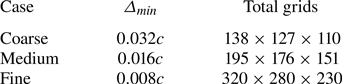
Three different sizes of grids are used here as listed in table 2. The size of the solid surface grid of the wing is chosen as the same as the fluid grid for each scenario. Twenty flapping cycles have been simulated, which is sufficient to ensure the flow field does not change significantly from cycle to cycle. Furthermore, the instantaneous force coefficients along the  $x$-axis (
 $C_x=2F_x/(\rho _o U^2_{ref} 1.5c^2)$,
 $F_x$ is the force along the
 $x$-axis) and
 $z$-axis (
 $C_z=2F_z/(\rho _o U^2_{ref} 1.5c^2)$,
 $F_z$ is the force along the
 $z$-axis) obtained from these three different grids are shown in figure 8 where the results from the medium and fine grids are closer with respect to that from the coarse grid. Therefore, it can be concluded that the medium grid is considered to be fine enough to calculate the flow field here. Here
 $\varDelta _{min}$ of 0.01
 $c$ will be used in all simulations to achieve a higher resolution at a reasonable cost.
Grid convergence study.
Grid convergence study: (a) instantaneous force coefficient in the  $x$-axis
 $C_x$ and (b) instantaneous force coefficient in the
 $z$-axis
 $C_z$, obtained from the coarse, medium and fine grids.

A.2. Computational domain convergence study
Two different computational domains were selected: (i) a small computational domain ( $10c \times 10c \times 10c$) and (ii) a large computation domain (
 $20c \times 20c \times 20c$). With the same grid resolution used in fine grid region (
 $\varDelta _{min}=0.01c$), the total grid points for these two domains are 11 362 000 and 25 740 000, respectively. The instantaneous force coefficients
 $C_x$ and
 $C_z$ (see figure 9) are insignificantly affected (less than 1 % variation). Therefore, the small computational domain is used in this work.
Computational domain convergence study: (a) instantaneous force coefficient in the  $x$-axis
 $C_x$ and (b) instantaneous force coefficient in the
 $z$-axis
 $C_z$, obtained from small and large computational domains.

A.3. Farassat formulation 1A validation
To validate the acoustic solver, the acoustic field generated by a 2-D periodic oscillating circular cylinder in a uniform flow with a prescribed motion in the  $y$ direction of
 $y(t)=0.1D\sin (2{\rm \pi} {\cdot }0.25t)$ is calculated. The Reynolds number (based on the velocity of the incoming flow
 $U_o$ and the diameter of the cylinder
 $D$) and the Mach number are 100 and 0.1, respectively. To compare the results from the current acoustic solver with those from the 2-D simulation, a spanwise extension of the noise sources (Singer et al. Reference Singer, Brentner, Lockard and Lilley2000) is used here. The r.m.s. of the sound pressure (normalised by
 $\rho _o$ and
 $c_o$) at (0,
 $50D$, 0) normal to the incoming flow is calculated by varying the spanwise extension length
 $L_c$ and shown in figure 10(a) where
 $p'_{rms}$ converges to
 $2.5 \times 10^{-5}$ at a large
 $L_c$ (e.g.
 $L_c/D>1000$). Therefore,
 $L_c=1100D$ is chosen here. The r.m.s. values of the sound pressure at
 $|\boldsymbol {r}|=50D$ from the current solver are in good agreement with that from Seo et al. (Reference Seo, Menon and Mittal2022) as shown in figure 10(b).
Sound pressure generated by a 2-D heaving circular cylinder at  $Re=100$ and
 $M=0.1$: (a) r.m.s. of sound pressure at (0,
 $50D$, 0) obtained from different spanwise extension length (
 $L_c$) and (b) r.m.s. of sound pressure at
 $|\boldsymbol {r}|=50D$ obtained from current solver with
 $L_c = 1100D$ and the results from Seo et al. (Reference Seo, Menon and Mittal2022) are used here for comparison.

A.4. Simplified model validation
To validate the simplified model [see (2.9)], the sound pressure generated by the hovering wing (see figure 2) at (100 $c$,0,0) and (0,0,100
 $c$) obtained from the simplified model is compared with that from the Farassat formulation 1A (see (2.6), results are transformed into the frequency domain via fast Fourier transform) in figure 11. The input for the simplified model and Farassat formulation 1A is the fluid data that are obtained from 10 flapping cycles and collected every 10 time steps (
 $10 \Delta t = 0.04$), yielding a resolution in the frequency domain of
 $\Delta \,St =0.025$. It can be seen that good agreement between these two methods has been achieved with some discrepancies at
 $2f_o$ for (100
 $c$,0,0) (see figure 11a), which may be caused by the fact that the
 $2f_o$ component dominants the noise at the sides (
 $y$- and
 $z$-directions). Overall, the simplified model with its low computational cost and excellent accuracy has proven that the time derivative of the surface pressure is the dominant noise source for the hovering wing at a low Mach number.
Sound pressure level (SPL) in the frequency domain at (a) (100 $c$, 0, 0) and (b) (0, 0, 100
 $c$), obtained from the Farassat formulation 1A and the simplified model,
 $St=f c/U_{ref}$.



