INTRODUCTION
Over the last couple of years, the study of behavioral models of dynamic interaction in financial markets has brought about a better understanding of some of the key stylized facts of financial data, in particular of the fat tails of the distribution of returns and the temporal dependence in volatility. Although these statistical features have counted as almost universal findings for practically all financial time series for a long time and appear to be extremely uniform across assets and sampling horizons, economic explanations of their behavioral origins were nonexistent until very recently. However, the recent rush of interest in heterogeneous agents models, the availability of fast computers for simulations of markets with a large number of agents, and the introduction of new analytical and computational tools (often adapted from statistical physics) in the analysis of multiagent systems have brought about quite a number of models in which the above stylized facts (one of them or both) have been shown to be emergent properties of interacting agent dynamics. Some of these contributions show that besides reproducing key statistical properties, the overall dynamics is also indistinguishable from a unit-root process. Hence, despite having identifiable behavioral roots (in terms of the assumed speculative behavior of the agents), no immediately recognizable traces of predictability can be found in the simulated time series, and the dynamics appears to be observationally equivalent to a martingale process.
Early papers in this area have often been the results of collaborations between economists and physicists, e.g. Takayasu et al. (1992), Palmer et al. (1994), and Baki et al. (1997). Although they made important contributions to getting this literature started, in some of these early papers the proximity of the resulting time paths to empirical data was quite limited. Later studies have merged this multiagent approach with the type of noise trader–fundamentalist interaction introduced by Beja and Goldman (1980) and Day and Huang (1990). Papers along this line included the microscopic stock market models of Lux and Marchesi (1999, 2000), Chen et al. (2001), Chen and Yeh (2002), Iori (2002), Farmer and Joshi (2002), and LeBaron (2000) as well as the adaptive belief dynamics of Gaunersdorfer and Hommes (2005) and Gaunersdorfer et al. (2000). A related approach can be found in the artificial foreign exchange markets of Arifovic and Gencay (2000) and Georges (2005), in which agents' selection of strategies is formalized via genetic algorithms.
Interestingly, some general conclusions seem to emerge from this literature. First, volatility clustering and fat tails may result from adaptive behavior in the presence of indeterminacy of the equilibrium of the dynamics [see Lux (2005)]. In particular, with different strategies performing equally well in some kind of steady state, stochastic disturbances lead to continuously changing strategy configurations, which every once in a while generate bursts of activity. This type of dynamics can be found already in Youssefmir and Huberman (1997) in the context of a resource exploitation model and can be identified in both the papers by Lux and Marchesi (1999, 2000) and the otherwise quite different GA models of Arifovic and Gencay (2000), Lux and Schornstein (2005), and Georges (2005).
Another more general avenue toward an explanation of these features can be found in Gaunersdorfer and Hommes (2005), who show that volatility clustering can emerge from stochastic dynamics with multiple attractors. Small amounts of noise added to a deterministic dynamics with two or more attractive states can lead to recurrent switches between these attractors. As these different regimes often have different levels of variability of the dynamic variables (e.g., a fixed point vis-à-vis a chaotic attractor), some degree of volatility clustering is a somehow natural result of such a process. Interestingly, both of these mechanisms are sometimes identified as examples of intermittent dynamics, which might, therefore, be thought of as a general conceptual framework for the explanation of the particular characteristics of financial markets.
Although the above models contain—due to their origin from the behavioral finance literature—more or less complicated descriptions of agents expectations and strategy choices, some authors with a physics background have rather tried to reduce the dynamics to a few basic principles able to generate the required time series characteristics. Recent models with only a few ingredients for activation and frustration of agents leading to realistic simulated output include those of Eguiluz and Zimmermann (2000), Bornholdt (2001), and variants of the so-called minority game [Challet et al. (2001)].
Our aim in this paper is similar to that of these studies. We are interested in whether an extremely simplified model of interaction of noise traders and fundamentalists is already sufficient to reproduce the key stylized facts: unit roots, fat tails, and volatility clustering. The model we investigate in this paper is a simple variation of the herding dynamics introduced by Kirman (1993) and Lux (1995). We distinguish between two groups and allow for mimetic contagion among agents by assuming that they will move from one group to the other with a certain probability depending on group size. This leads to the natural emergence of majority opinions, with all agents sharing one of two available opinions. However, the stochasticity of the dynamics also leads to recurrent switches between majorities, so that the model generates a bimodal ergodic distribution of the agents' configuration. With a simple price adjustment rule added, this bimodality carries over to prices as well. Simulations of this model show that it can mimic in surprising quantitative accuracy the above stylized facts. The simplicity of the model also makes it possible to derive some analytical insights into its dynamics. In particular, it is straightforward to show that the model does not exhibit “true scaling,” neither concerning the distribution of large returns, nor for the temporal dependence structure of volatility. This apparent scaling, in fact, results from a kind of “regime switching” between the two modes of its stationary distribution. This is a phenomenon similar to the difficulty of distinguishing between apparent and true scaling in certain stochastic processes (Anderson et al. 1999; Granger and Teräsvirta 1999; Diebold and Inoue 2001; LeBaron 2001). Our analysis thus demonstrates that “apparent” scaling is not confined to a particular class of appropriately constructed stochastic models, but might also prevail in behavioral approaches with interacting agents.
Closely related models have also been studied by Wagner (2003) and Alfarano et al. (2005a, 2005b). Whereas Wagner (2003) investigates a more complicated model in which agents are allowed to switch between three different groups, Alfarano et al. (2005a) elaborate on a model with two groups of traders similar to the present one and estimate its parameters for selected financial time series. Alfarano et al. (2005b) derive closed-form solutions for both conditional and unconditional moments of a similar model, which provide insights into the mechanisms generating the apparent power-law behavior.
The remainder of this paper is structured as follows: in Section 2 we introduce a simple model of contagion. Section 3 provides the details of the artificial market structure, in which we embed the contagion mechanism. Some analytical approximations of the return dynamics are also derived that provide us with important insights into the origin of leptokurtosis and temporal dependence in volatility. Section 4 contains a statistical analysis of simulated data demonstrating their close proximity to empirical records in the sense of scaling laws with “realistic” exponents. The finite sample properties of some of these tests are analyzed in Section 5 and compared to their known asymptotic behavior. As it turns out, apparent scaling occurs over a well-defined time horizon beyond which the “true” asymptotic behavior is recovered. Some final remarks conclude the paper.
A SIMPLE MODEL OF CONTAGION
Transition Rates
Our market is populated by N agents, each of them belonging either to group A or to group B. The numbers of agents in the two groups are denoted by NA and NB, respectively. The state of the system can be conventionally described by an intensive variable x:

The probability of observing a transition of the system during a time interval Δt0 from a configuration {NA, NB} to
will be denoted by

Because in the limit of continuous time, Δt0→0, multiple switches during one incremental time unit become increasingly unlikely, we can confine the analysis to the cases NA±1 and NB∓1 for sufficiently small Δt0. The conditional probabilities for changes of the configuration of agents are assumed to reflect herding tendencies in the following way:
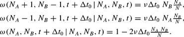
Equations (2) should be interpreted as follows: the probability of one agent switching from group A to group B per incremental time unit Δt0 is given by the probability of an A-agent being prone to a change of opinion (which we assume depends on the relative size of the B group, NB/N) times the number of A-agents in the population, NA. Vice versa, the probabilities for changes in the opposite direction are explained by analogous arguments. The constant ν is a parameter for the strength of contagion. In order to guarantee that on average only one agent will switch between groups, the elementary time step has to be constrained by the inequality

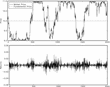
This model, therefore, formalizes interactions between economic agents (traders) based on imitative behavior. The contagion effect is modeled via the dependence of the transition probabilities on the fraction of traders in the alternative state. The perfect symmetry of equation (2) could suggest a similarly symmetric outcome of this dynamics. However, this is only partially correct, as the outcome of the process is a temporary polarization of opinion among the traders (see Figure 1), although the equilibrium distribution of x turns out to be symmetric around 0.

The upper panel shows the behavior of the fundamental (simply assumed to be constant) and the market price from a typical simulation. The lower panel shows the returns of the market price, computedas log increments over unit time intervals. Underlying parameters of this run are N=100, ν=1, pF=10.The simulation is performed using the binomial updating method from equations (A.4) and (A.5).
Taking stock of equation (1), NA and NB could be expressed as

Expressing the probabilities (2) in terms of x, we end up with1
We use now the more compact notation ω(x→x+Δx) to indicate the conditional probabilities from equation (2).
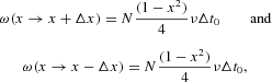
and obviously

with the elementary step of the variable x being Δx=2/N. In this setup, x=−1 and x=1 are absorbing states in which no change of the population can occur any more. To avoid the total extinction of one group, we introduce reflecting boundary conditions (RBCs hereafter) at the edges:

The previous probabilities together with the RBCs for the realizations of x specify a finite and homogeneous birth–death process [see Chapter 1 in Kelly (1979)]. The two states |x|=1 are now transient rather than absorbing states, so that their equilibrium probabilities are identically zero (Pe(|1|)=0), because they could not be reached from any other state and, if they happened to be chosen as initial conditions, the system would never return to these states. If we exclude the states |x|=1, the resulting finite Markov chain is ergodic, because it is aperiodic and irreducible.2
The chain is aperiodic because the conditional probability of remaining in the state is strictly positive for all states. It is irreducible because every state can be reached from another arbitrary state in a finite number of steps.
Equilibrium Distribution
To derive the functional form of the equilibrium distribution Pe(x), we adopt the following strategy: we assume that for our Markov chain the detailed balance condition

holds for a particular weighting function w(x), which we assume to be strictly positive in its domain and to sum up to one. If the detailed balance condition holds, w(x) coincides with the equilibrium distribution Pe(x), given the ergodicity of the chain. Therefore, if w(x) indeed can be shown to exist and if it can be derived in closed form, we have proved that the detailed balance condition holds for our model and we have at the same time recovered the functional form of Pe(x).
Because we assume that w(x) is strictly positive, we can write w(x) as an exponential function:

By means of equations (4) and (5), we obtain

For large N, we can rewrite equation (6) in the limit Δx→0, which results in a simple differential equation for U(x),

which we can easily solve for U(x):

The equilibrium distribution is then given by
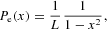
where L is its normalization constant,

with δ=1/N (we explain in detail in Section 3.2 below why the boundaries of the integral are −1+1/N and 1−1/N). Given that the weighting function w(x), defined in (4), exists, the detailed balance condition holds and the Markov chain is, therefore, time-reversible. Time-reversibility of the Markov chain implies that the probability of a transition from a state x0 to any other state of the chain x depends solely on x and x0, but not on the particular path. In other words, the equilibrium properties of the chain are invariant under a reversal of time [see Chapter 1 in Kelly (1979)].
It is easy to obtain the second and fourth moments of x, which are, respectively, given by (see Appendix A.3 for details)
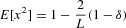
and

The previous mechanism is obviously inspired by Kirman's analysis of opinion formation (Kirman, 1993). The main difference from Kirman's model is the absence of a constant term in the transition probabilities (2), introduced by the author to prevent the existence of absorbing states at |x|=1. We have replaced this ingredient by imposing reflecting boundary conditions, which similarly prevent a lock-in at one state with all agents following one of the two behavioral alternatives. As a consequence, the only possible scenario in our case is a distribution with mass concentrated in the extreme values (U-shaped distribution), whereas in the original model a flat distribution and a distribution with a unique mode at zero are also possible, depending on the particular values of the parameters. Alfarano et al. (2005a) have investigated another variant of the Kirman model, allowing asymmetric unconditional distributions. In their model the constant parameters in the transition probabilities are allowed to assume different values for switches in one or the other direction. This enhanced flexibility of their model allows a wide spectrum of outcomes of stationary population distributions and the associated return distributions derived from them.
THE FINANCIAL MARKET MODEL
Agents' Behavior
We now use this two-state opinion dynamics as the main ingredient in a financial market model with interacting heterogenous agents. Our market participants are divided into two groups:
NF fundamentalists (F), who buy (sell) a fixed amount of stocks TF when the price is below (above) its fundamental value pF;
NC noise traders (C), who are driven by herd instincts.
Assuming sluggish price adjustment by a market maker in the presence of excess demand, the price dynamics can be formalized by

where β is the speed of price adjustment.
As an approximation to the resulting disequilibrium dynamics, we may consider instantaneous market clearing (Walrasian scenario). We can, then, solve (11) for the equilibrium price:
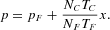
Without loss of generality, we simplify notation by choosing the following set of parameter values:

Due to equation (12), the average price is pF because the mean of x is zero. We can observe, however, phases in which the asset is undervalued (compared to the fundamental price) alternating with episodes in which it is overvalued. In the first case the majority of the noise traders is in the pessimistic group, whereas in the second case most of them are in an optimistic mood.
We define the returns as the log-increment of prices over an arbitrary time interval,3
Note that the time increment Δt is arbitrary and does not necessarily coincide with the time unit Δt0 used in the formalization of transition probabilities (2). We will see in the next section that a careful choice of Δt leads to a meaningful approximation of the dynamics of the variable x.

where the last approximation holds as long as |x|/pF [Lt ] 1.
Simulation Results and Analytical Approximations
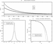
As it turns out, our simple model is able to reproduce some of the salient characteristics of financial markets. Figures 1 and 2 illustrate the results of the model. Volatility clusters are visible in the time series of returns and the unconditional distribution of returns is leptokurtic. The autocorrelations of absolute and squared returns (as a measure of volatility) are positive over an extended time horizon, while the raw returns show almost no correlation. All these features are in qualitative agreement with empirical findings.
In addition to our Monte Carlo analysis of the simulated data, detailed in Sections 4 and 5 below, we can provide some analytical results for the dynamics of the opinion index x and the associated returns. In Appendix A.2, we show that the dynamics of the discrete variable x can be approximatively characterized by the recursive stochastic difference equation4
Equation (13) is a meaningful approximation of the dynamics of the discrete variable x if we can treat it as a continuous variable. The approximation holds if both NO and NP are large, and therefore not too close to the boundaries |x|=1−δ. Closer to the reflecting boundaries, in fact, the discrete nature of the process remains important even for large N. Note that during the macroscopic time increment Δt multiple switches are allowed; cf. Appendix A.2.

where η(·) is a random variable drawn from a standard normal distribution. The previous equation is called the Langevin equation in the pertinent literature. Note that because of the Gaussian approximation of the noise term, we cannot exclude values of the variable x outside its admissible domain |x|<1−δ. Therefore, equation (13) has to be supplemented by reflecting boundary conditions, which are conveniently formalized as (cf. Appendix A.1)


which establish the behavior of x in the nonpermitted region. Moreover, note that equations (14) and (15) are equivalent to a reflection around the points x=−1+1/N and x=1−1/N. The domain of the variable x in the continuous approximation, therefore, extends to the interval
. This determines the value of δ=1/N in equation (8).
Because
, the approximation (13) is extremely useful in analyzing the dynamics of returns. First, equation (13) reveals that heteroscedasticity in the returns series is due to the nonlinear state-dependent diffusion term, which directly derives from the Markovian herding interaction among traders. The diffusion term, in fact, vanishes at the edges (|x|≈1) and attains its maximum at x=0. Moreover, by means of equation (13), we can compute the variance and kurtosis of the return distribution,

and
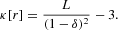
All the odd moments are identically zero, given the symmetry of the system. It can be verified that the resulting return distribution is leptokurtic (i.e., κ>0) for any number of noise traders.5
From equation (17) we notice that for any number of agents N the distribution of returns is leptokurtic. However, because equation (17) has been derived under the assumption of large N, this conclusion has to be treated with caution.
Plugging in the pertinent values pF=10, ν=1, and N=100, we have E[r2]=3.741×10⁻⁵, and κ=2.401.
Note that autocorrelations for raw returns are identically zero for all time-lags, due to the absence of a drift term in equation (13) and the independence of the Gaussian noise. To compute the correlation of higher moments, for example squared and absolute returns as a proxy for the volatility, is a more cumbersome task. Note that equation (13) does not include the effect of the reflecting boundaries, which play a crucial role in the dynamics of the model. It should, therefore, be obvious that the reflecting boundaries would add some element of mean-reversion to the approximate law of motion (13). To compute exact autocorrelation formulas for both raw returns and absolute or squared returns, one would have to include the effect of the RBCs in the dynamics. Unfortunately, we have not been able to derive these autocorrelation functions analytically. We rely, therefore, on Monte Carlo simulations of the process (13) together with equations (14) and (15). Figure 2 shows the slow decay of the autocorrelation of both absolute and squared returns, together with the almost complete absence of autocorrelation in raw returns. The approximatively exponential decay of these autocorrelation functions is not surprising, given the Markovian nature of the underlying process.

(a) Autocorrelation function of raw, squared, and absolute returns. (b) Distribution of normalized returns compared to a standard normal distribution; notice the leptokurtic shape. (c) Inverse cumulative distribution. Parameters: N=100, ν=1, pF=10, number of observations 3 × 10⁵.

It is also worthwhile pointing out that the analytical structure of the stochastic equation governing the dynamics of returns falls into the wide class of stochastic volatility models employed in financial econometrics. However, note that in contrast to phenomenological models of volatility, our model has been derived from a behavioral approach of interacting agents, albeit a very simple one. It could therefore be viewed as a bridge between the econometric and agent-based models of asset price dynamics.
Mean first passage time
Under a proper choice of the time interval Δt (see Appendix A.2), the dynamics of the system can be modeled via the Langevin equation given by equation (13), where the drift and diffusion functions are given by

The equilibrium distribution (7) is bimodal, with two modes at |x|=1−δ due to the reflecting boundary conditions. The system can be described as “bistable” with two “equilibria” coincident with the modes. However, we might observe transitions between them with finite probability. The average time needed for a transition is denoted as the mean first passage time T0, which can be computed using the textbook formula [see Gardiner (2003, p. 139)]

where
. The integral (19) can be computed explicitly, leading to7
With the chosen parameters N=100 and ν=1, we obtain T0 ≈ 1,060.

STATISTICAL ANALYSIS OF SIMULATED DATA
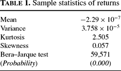
To see how closely the statistical results from our simulated data match empirical observations, we performed a series of experiments with a long data set of 1,000,000 integer time steps. Tables 1 and 2 give some elementary statistics for the whole sample. As can be seen, the resulting distribution is characterized by significant excess kurtosis and slight positive skewness. The Bera–Jarque test for normality leads to a strong rejection of its null hypothesis.
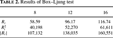
To investigate the autocorrelation structure, we applied the Box–Ljung test to auto-correlations of up to 8, 12, and 16 lags for the raw data as well as the squares and absolute values of returns. In harmony with empirical records, there is only slight autocorrelation in the returns themselves, but highly significant autocorrelation in the squares and absolute values. Because, with samples of that size, we are able to detect even very small degrees of autocorrelation with high reliability, we would not expect the results of the Box–Ljung test to be insignificant (in fact, they allow rejection of the null of no autocorrelation even for the raw returns, presumably due to the influence of our reflecting boundaries). However, what is interesting here is that the statistics are orders of magnitude larger for the squares and absolute values of returns.
The highly significant entries for the latter transformations lead to the question of whether these time series are able to mimic the empirical observations of long-term dependence, defined as hyperbolic decay of the autocorrelation function,

where γ is the decay parameter. To this end, we estimate the parameter of fractional differentiation, denoted by
, from a regression in frequency space following the approach of Geweke and Porter-Hudak (1983) (GPH), as well as the Hurst exponent
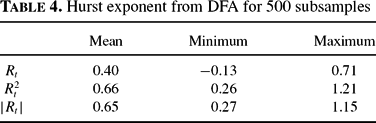
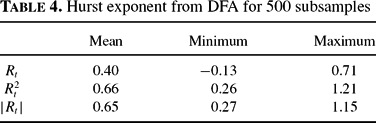
from detrended fluctuation analysis (DFA) (Peng et al. 1994); see Tables 3 and 4

The GPH method is based on the linear regression of the log-periodogram on transformations of low frequencies of the Fourier spectrum. The estimated parameter d is related to the decay rate of the autocorrelation function by

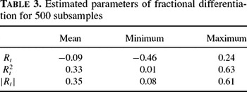
A value of d = 0 would indicate the absence of long memory, whereas d significantly above zero speaks in favor of long-term dependence. Table 3 gives summary results from 500 sub-samples of 2,000 observations each. As it turns out, we get results in the vicinity of zero for the raw data, but on average much higher values for the squares and absolute returns. In fact, the latter are very close to typical empirical estimates obtained with returns of various financial markets [cf. Lux and Ausloos (2002)].
Estimates from the alternative DFA approach (shown in Table 4) confirm these results. Note that the theoretical relationship between the two coefficients is

We observe that for both methods we find satisfactory agreement for raw returns. For absolute and squared returns, results from both methods are qualitatively similar, albeit with a larger difference in the numerical values. The later might be explained, however, by different small-sample biases of the two estimators.
The appearance of long-term dependence is particularly interesting because simple inspection of the model, in fact, indicates that it does not exhibit this feature: Figure 2 indicates that the absolute and squared returns are characterized by approximately exponential decay of their autocorrelation function, which is, in fact, the defining property of short-memory processes. This property does not come as a surprise given the Markovian nature of the underlying stochastic process (3). However, it is known that certain classes of regime-switching models can indeed “erroneously” give the impression of long-term dependence [Lobato and Savin (1998); Anderson et al. (1999); Granger and Teräsvirta (1999); Diebold and Inoue (2001)]. Because switching between the two modes of the distribution in our model is similar to changes of regime in Markov-switching models, we conjecture that the source of apparent long-term memory should be closely related to these findings in the statistical literature. Interestingly, a similar result can be found in Kirman and Teyssière (2002), who study a more complicated foreign exchange market model in which Kirman's herding model is combined with a monetary approach à la Frankel and Froot (1986).
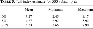
We now turn to the unconditional distribution of the synthetic data. To complement the results for kurtosis, we estimate the so-called tail index to get an assessment of the heaviness of the tails of the simulated returns. Empirical research indicates again a hyperbolic relationship for the decay of the probability in the outer part of the return distribution, following

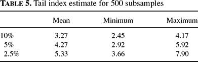
with α usually in the range of [2.5, 5] [cf. Lux and Ausloos (2002)]. Here we applied the usual maximum likelihood estimator proposed by Hill (1975), using the same 500 sub-samples and tail sizes of 10, 5 and 2.5%. Both the range of the estimators and the tendency toward slightly increasing numbers are in good harmony with empirical results (see Table 5).
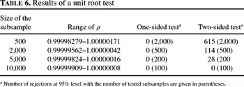
The martingale behavior of financial data is another well-established stylized fact, cf. de Vries (1994), usually interpreted as a consequence of informational efficiency. In other words, one is typically not able to reject the null hypothesis that the price follows a unit root process. To test for a unit root, we applied the standard Dickey–Fuller test to subsamples of different lengths (from 500 to 10,000; see Table 6), in order to check whether the simulated time series show the same pattern as empirical data.

As can be seen from Table 6, we cannot reject the null hypothesis of a unit root using a one-sided test for all the subsamples considered. In contrast, applying a two-sided test, we observe several cases of rejections in favor of an explosive root of the dynamics. Inspection shows that these cases are driven by switching between the two modes of the distribution in the pertinent subsample. The fast change of the majority of the noise traders creates the impression of an exponential increase of the price (leading to an estimated autoregressive parameter ρ>1) for particular choices of the size of subsamples, even though the time series of the price is bounded. However, with longer sample sizes we observe fewer rejections also for the two-sided test, because the time series then runs over several transitions between the two “equilibria.”
DISCOVERING THE ASYMPTOTIC BEHAVIOR
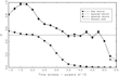
The incongruity between the theoretical properties of the model (absence of long memory) and the results of the statistical investigation, described in the previous section, in the end should be a “finite size” effect (even though one might recover the “true” behavior only with immense amounts of data). To show the transition toward its true behavior in the case of apparent long-term dependence of volatility, it is necessary to study the asymptotic correlation properties of the time series. To this end, Figure 3 shows the Hurst exponent, estimated via DFA, as a function of different time windows (ranging from 10 to 5×10⁵ time steps Δt) for raw, squared, and absolute returns.

Estimated Hurst exponents for raw, squared and absolute returns for different time windows calculated via detrended fluctuation analysis. The dashed line isthe benchmark value for a random walk. Note that for our numerical example, T0 ≈ 1,060 for N=100.
Concerning the raw returns, we observe a vanishing Hurst exponent, which after its initial fluctuations around 0.5 eventually approaches zero for longer time windows. This behavior can be explained by the boundedness of the time series of the price, which leads to constant variance of returns. Since the Hurst exponent measures the rate of increase of the variance, it therefore has to decline toward zero for large time horizons. But if we restrict our time horizon to a few hundred or thousand time steps (with the extent of the preasymptotic regime depending on parameter values), the Hurst exponent stays close to 0.5, the value of a random walk.
The estimate shows different properties for the time series of squared and absolute returns. For moderate time horizons, both exhibit values above 0.5, which would be characteristic of long-memory processes, whereas from about ∼104 time steps, the Hurst exponent declines to the typical value of the random walk; and at the end we observe a convergence to zero that is indicative of a bounded time series.
The explanation of these results lies in the oscillatory pattern of the price. These oscillations create a characteristic time scale T0 [see equation (20)], below which the time series is indeed close to a random walk, with a linear increase of the variance over time. This is exactly the time scale over which the difference equation (13) provides a good approximation of the dynamics. The zero drift of this equation is, in fact, in perfect harmony with the pseudo-empirical result of nonrejection of a unit root and a Hurst coefficient of 0.5 for raw returns. However, for longer time series (the size of the sample T several times greater than T0), the switching between the two modes becomes important and the variance reaches a constant value because it then averages over numerous oscillations between the two modes. These oscillations have the character of regime-switching dynamics alternating between a calm period and a turbulent one, which is observationally similar to a long-memory process, at least for time windows not too large compared to T0. This effect seems to be responsible for the spurious estimates H > 0 for squared and absolute returns, when the size of the sample is no too long.
The time scale T0 therefore determines the necessary number of data for recovering the true behavior of the model. Samples of smaller size, on the other hand, give rise to different “spurious” characteristics, which are, in fact, in good agreement with the empirical data; from (20) we can even calculate the scaling of the necessary sample size depending on the parameters of the model.
CONCLUSIONS
This paper has analyzed an extremely simple variant of a noise trader/infection model. In contrast to many other contributions to the literature on artificial financial markets, it belongs to a class of models whose dynamical behavior is well understood. In particular, we know that it amounts to a bounded Markovian process with a bistable limiting distribution, and therefore, the model should lack any true scaling properties. Nevertheless, applying the usual statistical tests to simulated data, we find apparent scaling with quite close agreement with empirically observed exponents. This shows that the difficulty of distinguishing between true and spurious scaling is not confined to particular stochastic processes, but may also emerge in behavioral multiagent models. Our analytical approximations, in fact, show that apparent temporal scaling laws would be the typical outcome of simulations of pseudoempirical tests as long as the sample sizes are below a critical threshold T0. We argue that such apparent scaling might also occur in other models that have been proposed in the literature.
APPENDIX
SIMULATION ALGORITHM
The contagion process formalized in Section 2 belongs to the class of continuous-time-jump Markov processes. Simulating this process, one has to find an appropriate compromise between the proximity of the discrete simulations to the underlying continuous time dynamics and the efficiency of the simulation algorithm. A convenient approach to the joint dynamics of an ensemble of traders consists in simulating the agents' transitions between groups by binomial draws. To this end, we consider a macroscopic time scale Δt[Gt ]Δt0, which, however, should also not be too long, so that the main features of the dynamics are preserved in this approximation.
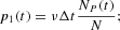
In line with the contagion process formalized in equation (2), we can also formalize transition probabilities for individual agents. Each optimistic agent has a probability of changing attitude over the unit time interval Δt given by
conversely, every pessimist can switch to the group of optimists with probability
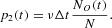
The probabilities (A.1) and (A.2) impose the condition

for a feasible simulation algorithm that imposes an upper bound on the admissible time-increment Δt one could use in the simulations. Note that here during the time unit Δt in this discrete approximation of our continuous-time model, we might observe multiple switches of agents between the two states. Although the time unit Δt is constrained by the previous inequality, its value is, in principle, arbitrary. The time evolution of the number of traders in the two groups is, then, given by

and

where B(·, ·) represents a random variate drawn from a binomial distribution. The signs in front of the random variables represent the agents' movements in and out of each group. The dynamics governed by equations (A.4) and (A.5) have to be complemented by the RBCs to avoid absorbing states NO,P=0; that is, at least one agent should remain in each group. Moreover, given the independence of the two binomial draws in equations (A.4) and (A.5), we have to take into account the possibility of negative values of NO(t) and NP(t) resulting from the dynamics of equations (A.4) and (A.5). To reinitiate the dynamics after a violation of the RBCs, we conventionally add the following rules to the above difference equations:

and

Note that the previous conditions imply a reflection around the points NO,P=0.5, which is equivalent to
in terms of the intensive variable x. This explains the boundaries that have been imposed in equation (8).
DERIVATION OF THE LANGEVIN EQUATION (13)
The basic idea of the Langevin approximation is to find a time horizons for which the conditional distribution of the discrete variables NA and NB is well approximated by a Gaussian. To do so, we have to carefully define the time unit Δt that we use in equations (A.4) and (A.5). For notational convenience, let us define nt as the number of optimists in the market at time t, and N−nt as the corresponding number of pessimists. First, we may approximate the two binomial distributions in equation (A.4) by two normal distributions. One might recall that a binomial distribution B(M, p) can be well described by a Gaussian with mean Mp and variance Mp(1 − p) in the case of a large number of “Bernoulli trials” M [see for instance Feller (1971)], and, additionally, if Mp[Gt ]1. In our case, we are allowed to use this approximation if N − nt and nt are large, and p1· nt[Gt ]1 and p2·(N − nt)[Gt ]1. This means that the approximation should work reasonably well if nt is far from its boundaries and νΔt∼O(1), according to equation (A.3). Hence, the Langevin approximation should work well under the assumption of a large number of agents, if we are not too close to the boundaries and if we fix the arbitrary time scale to be Δt∼O(1).
We can, then, rewrite equation (A.4) as

where η and ξ are independent random normal variables. Given equations (A.1) and (A.2), we obtain ntp1=(N−nt)p2. Note that, on average, the numbers of agents switching in both directions are identical, so that the agents' expected outflow from each state offsets the corresponding inflow at every instant t. What remains is just the contribution given by the fluctuation terms. We therefore arrive at

Because the sum of two independent normal variables η and ξ with mean zero and variances
and
, respectively, is still a Gaussian variable (ζ) with variance
, we can further simplify equation (A.8) and end up with

Expressing the numbers of agents nt+Δt and nt in equation (A.9) in terms of the intensive variables xt and xt+Δt as

we obtain the final result given by equation (13) in the main text.
MOMENTS OF x AND r
The computation of the second moment of Pe(x) yields the following result:

The fourth moment can be computed via the integral decomposition

which leads to equation (10) in the main text.
By means of the recursive equation (13) and the second moment of x from (9), we can easily compute the second moment of the return distribution p(r):

Plugging equations (9) and (10) into the previous expression, we have the fourth moment given by

The computation of the kurtosis is, then, straightforward using the previous two results.
MEAN FIRST PASSAGE TIME
Plugging equation (18) into equation (19), we end up with equation

The second integral is given by

The first term is vanishing altogether and the integral of the second term yields

Plugging the previous result into equation (A.10), we obtain equation (20) in the main text.
We are particulary grateful to Jean-Philippe Bouchaud and Friedrich Wagner for helpful suggestions and intense discussions during the preparation of this paper. Financial support by the European Commission under STREP Contract 516446 is gratefully acknowledged. We also gratefully acknowledge financial support by the Deutscher Akademischer Austauschdienst and the Landesbank Schleswig-Holstein. A preliminary version of this paper appeared in the volume Long Memory in Economics, edited by Gilles Teyssière and Alan Kirman (pp. 345–362; Berlin: Springer, 2005).