Nomenclature
- X
Scalar position
- V
Velocity
- A
Acceleration
- R
Position vector
- W
Rotational speed vector
- AC
Aircraft
- NED
North (x), East (y), Down (z) coordinate frame, with the centre on aircraft's centre of mass
- Inertia
Inertial coordinate frame, here assumed to be the same as NED
- Ra/b
Ra – Rb
 $C_I^B$
Rotation matrix, converting a vector in inertial coordinates to body coordinates
- V|cam
Velocity vector in camera coordinates
- h
Pixel position
- x, y, z
Position of point in camera coordinates
- u, v
Normalised pixel positions u = x/z, v = y/z
- N
Number of image rows
- ox, oy
Pinhole model offsets (in pixels)
- fx, fy
Pinhole model focal lengths (in pixels)
- k 1, k 2, k 3
Radial coefficients in Brown distortion model
- p 1, p 2
Tangential coefficients in Brown distortion model
- dr
Radial distortion in Brown distortion model
- dt
Tangential distortion in Brown distortion model
- td
Delay in capturing the centre of the image
- tr
Delay difference in capturing of the first row to the last one
- te
The exposure time of each pixel

1. Introduction
Data collection is an important phase in most research projects. A viable algorithm should perform well (or better) on the collected data. For algorithms to be comparable, common realistic data should be available. These data are provided using real recorded data (datasets), recorded data from scaled normalised environments (like wind tunnels), and computer simulators.
In the field of image processing and computer vision, recorded datasets are used more frequently than simulators and scaled environments due to the ease of recording camera images and videos. This can be a limiting factor when algorithms are supposed to work on airborne objects. Airborne recorded data are rare, incomplete, and hard to obtain in various flight conditions. The available airborne datasets use two types of camera. One is the fixed-zoom global-shutterFootnote 1 progressive camera, e.g., Kagaru airborne dataset (Warren et al., 2012), European Robotics Challenge micro aerial vehicle (EuRoC MAV) dataset (Burri et al., Reference Burri, Nikolic, Gohl, Schneider, Rehder, Omari, Achtelik and Siegwart2016) and an oblique camera in the Field and Service Robotics 2015 Autonomous Systems Laboratory (FSR 2015 ASL) dataset (Oettershagen et al., Reference Navarro, Serón and Gutierrez2016). The other is a rolling shutter camera without calibration, as in the UAV123 dataset (Mueller et al., Reference Meilland, Drummond and Comport2016) or the FSR 2015 thermal and nadir-looking high resolution camera. In the case of airborne RGB-D (Red-Green-Blue + depth) cameras, they are further limited to operational min/max depth limits (Huang et al., Reference Huang, Bachrach, Henry, Krainin, Maturana, Fox and Roy2017) and void areas (Pomerleau et al., Reference Pham and Suh2012).
Image generation by filming scaled environments appeared early in the movie-making industry, where it was used for special effects. It enabled the first image generators that were used for navigation (Koch and Evans, 1980) and training (Beard et al., Reference Beard, Buchmann, Ringo, Tanita and Mader2008). A miniature camera moved along a ‘terrain board’ which produced realistic onlineFootnote 2 videos for training pilots. Although these image generators saved the cost of real flights, they lacked the real artifacts that exist in images from real cameras. They also needed costly handmade replicas of the environments.
Image simulators were developed more recently. As camera simulators are mainly developed in the gaming, training and dynamic simulation industries, it is usually sufficient to simulate an ‘ideal’ camera. The term ‘ideal’ means there are no existing distortions, including geometric (lens effect), temporal (rolling shutter, motion blur, interlacing) and photometric (vignetting, light intensity, noise). With these simulation engines, the emphasis is mostly on environmental conditions like light level, shadows and weather conditions (OpenSceneGraph Library, Reference Oettershagen, Stastny, Mantel, Melzer, Rudin, Gohl, Agamennoni, Alexis, Siegwart, Wettergreen and Barfoot1998; Unreal Engine, 1998).
There have been some dedicated airborne camera simulators built on top of these engines for visual processing evaluations. They mostly did not model any distortion (Allerton, Reference Allerton2009; Atashgah and Malaek, Reference Atashgah and Malaek2012; Mueller et al., Reference Meilland, Drummond and Comport2016). Some of them modelled a few artifacts like sun shadows – e.g., FlightGear Flight Simulator (1997), AirSim (Shah et al., Reference Schumaker2018) or that proposed by Jiang et al. (Reference Jiang, Li, Gu, Sun and Xiao2019) – but still used ideal cameras. Only a few modelled fixed-zoom lens distortion (Koenig and Howard, Reference Koch, Evans and Wiener2004; Hempe and Rosmann, Reference Hempe and Rosmann2015; Yu et al., Reference Yan, Wang and Zhou2017). Other distortions were mostly ignored; exceptions are Atashgah and Malaek (Reference Atashgah and Malaek2013) who added motion blur to be eliminated in a mono-slam system, Irmisch et al. (Reference Irmisch, Baumbach, Ernst and Börner2019) who also added motion blur, and Pueyo et al. (Reference Pomerleau, Liu, Colas and Siegwart2020) who added out-of-focus/depth-of-field simulation to the AirSim simulator.
The majority of commercial state of the art cameras (like those for thermal or high resolution imaging) are still rolling shutter cameras, even with analog outputs (so interlaced). Due to the speed and vibration of the aircraft platform, airborne cameras usually amplify rolling shutter, motion blur and interlacing effects. These artifacts are not easy to remove, especially when they interact. Algorithms like visual odometry can be very sensitive to interlacing or even a slight rolling shutter, as discussed in Engel et al. (Reference Engel, Koltun and Cremers2018). The sensitivity of a wide range of visual processing algorithms to the amplified image distortions on an airborne platform brings about the need for a simulation environment. Unfortunately, no imperfect camera simulators (simulating rolling shutter, motion blur, interlacing, variable zoom lens distortion, vignetting, light level and image noise) suitable for generating airborne data have been developed so far, to the best of the authors’ knowledge, and this is the main motivation for this work.
In this paper several innovation points are proposed to solve the above-mentioned problem. The first innovation is a motion tracking algorithm allowing the user to reconstruct an eligible flight path according to the discrete flight log. A novel insight into the existing square root (SQRT) controller is also provided. The next and main contribution is the introduction of a short-time pixel displacement model, usable in a reverse pipeline. It is shown that in the reverse pipeline the inverse lens distortion and the inverse temporal distortions are decoupled, allowing the user to add even high values of lens distortion alongside the temporal distortion model. The developed post-processing shader program is published in a public repository (Mahmoudi, Reference Koenig and Howard2020) to simplify further development and usage of this paper.
This paper is as arranged as follows. The general problem is described in Section 2. To simulate a camera, its positions and velocities are needed at the camera frequency. This is discussed in Section 3. To add distortions, development of an ‘ideal’ base camera output and a depth map is discussed in Section 4. These two camera frames and the vignetting map, as well as linear and rotational speeds, distortion and zooming parameters, are passed to a post-processing shader which adds the geometric (Section 5), temporal (Section 6) and photometric distortions (Section 7). Results, tests and evaluations are discussed in Section 8.
2. Statement of the problem
Camera distortions are categorised as geometric, temporal and photometric. Geometric distortions are those that cause (static) physical movement in pixel locations. They are mainly caused because cameras with lenses do not exactly obey the pinhole model (refer to Section 4). Temporal distortions are those that cause timeshifts in the capture time of pixels (e.g. time delay, rolling shutter, motion blur, interlacing etc.). Photometric distortions are distortions added to pixel colour and intensity (light level, noise, vignetting, saturation, etc.).
Here we should describe shaders to show why all the direct distortion equations (at least for geometric and temporal distortions) have to be inversed in this paper. The operation of converting the sample data to realistic images, usually performed on a graphical processing unit (GPU), is called ‘rendering’ and the program doing that is called a ‘shader’. Shaders are available in two major subgroups, vertex and fragment. These are both parallel units of execution in GPU. Vertex shaders output corner positions (vertices) which form a polygon. This polygon is filled with pixels coloured by fragment shaders. In short, vertex shaders determine the geometry and fragment shaders determine the colour of pixels. As a polygon contains much higher numbers of surface pixels than corners, fragment shaders are built more efficiently in parallel execution.
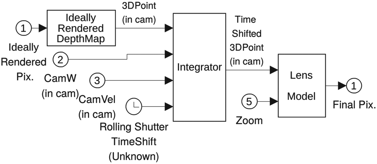
This paper proposes a two-stage shader. The first shader renders an ‘ideal’ snapshot of the environment as a reference. It contains colour and depth channels. Notice that this is a standard shader and can be replaced by any sophisticated off-the-shelf ideal camera simulator with depth channel, like Gazebo or AirSim. To cause distortions, a connection is needed between each pixel in the final distorted image (output) and the ideally rendered pixel from the previous stage (input). The colour and depth values in the distorted image are transferred based on this relation in a second shader. This second stage can utilise two approaches. One direct approach is to use a vertex shader via every snapshot pixel, determine its new position after distortion, and draw on it (Figure 1). Pixel location in ideal image (1), its depth, camera rotational speed (2) and linear speed (3) along with the timeshift (4) are input so that the integrator determines each pixel's three-dimensional (3D) position after temporal distortion. Lens distortion is added afterwards using the lens zoom (5). Although it is straightforward, there is no guarantee that every pixel in the output image will be filled, as many input pixels would map to the same output pixel. Modelling the rolling shutter and motion blur is also hard in this way. In the case of rolling shutter cameras, the exact timeshift based on the final (distorted) pixel location is not known beforehand. An iterative approach can be used, but it involves repeating whole calculations. Modelling motion blur also needs another repeat and averaging on whole calculations. This approach is not exactly parallel as many points may incorporate in forming a single pixel. Finally, by using vertex shaders per pixel on a GPU, this approach is not as parallel and fast as a fragment shader.
Direct approach, adding geometrical distortions to an ideal frame

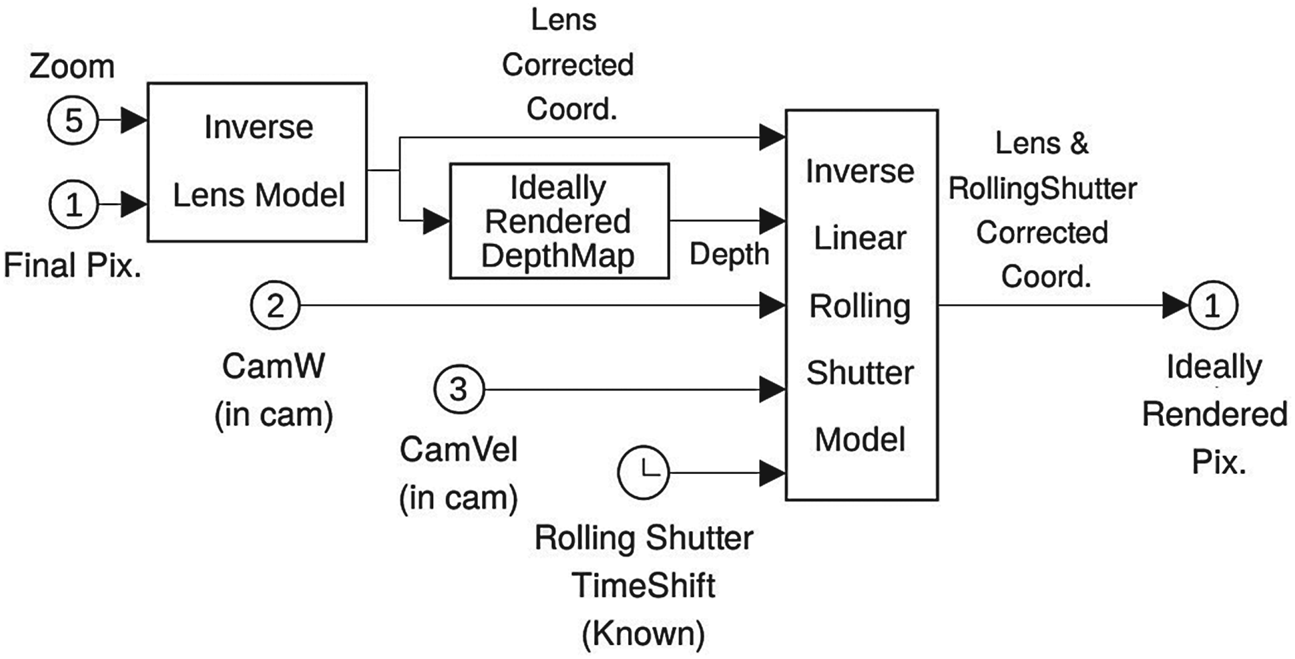
The other solution, the inverse approach, is to consider each output pixel position and reach its colour in the ideal snapshot by removing the distortion (Figure 2). Using the distorted pixel location (1) and lens zoom (5), the geometric distortion is removed first. By doing so, the geometric and temporal distortions are decoupled. Assuming the timeshift does not affect the depth, the 3D point position is calculated. This along with camera speeds (2, 3) and timeshift (4) is input to the inverse rolling shutter model to reach the ideal coordinates of the point. It gives a smooth image as it guarantees that every pixel in the output would have a colour (at least for those which map to valid pixels in the input image). Timeshift caused by the rolling shutter is a function of distorted pixel position which is known exactly. The motion blur can also be modelled efficiently as only a fraction of the algorithm is recalculated for getting the timeshift samples (inside the inverse rolling shutter model). This approach is completely parallel as the value of each output pixel can be found independently. On a GPU, a fragment shader can be used conveniently to render pixels in parallel. The only difficulty is that all the distortion models have to be inversed (analytically or numerically). This forms the root of some of the problems tackled in this paper.
The inverse approach, removing distortions from a distorted frame (inverse pipeline)

3. Aircraft track (flight path) generation
Aircraft (angular and linear) positions are directly used in the frame generation process. To model rolling shutter and motion blur, aircraft (angular and linear) velocities are also needed. The camera model needs this information in its own frequency. Unwanted discontinuities in position or velocities produce jumps in consequent frames and are not allowed. Out of range velocities would also cause extremely distorted or torn frames.
We assume the flight path of an aircraft (track) is provided by a flight log, which is a sparse table of aircraft positions and angles.Footnote 3 This approach is more flexible than using a dynamic flight simulation, as in Atashgah and Malaek (Reference Atashgah and Malaek2013), because it is not limited to a fixed type of aircraft. A ‘good’ trajectory would pass provided points as close as possible, maintaining a continuous track both in position and velocity, while fulfilling maximum speed and acceleration constraints. A simple linear interpolation between provided points to obtain data in camera frequency creates a velocity discontinuity at the provided points which is not applicable. A simple differentiation on the interpolated data to obtain velocities is also not applicable due to the noise present in the input data.
Several works have been done to generate acceptable trajectories. In Yan et al. (Reference Warren, McKinnon, He, Glover, Shiel, Yoshida and Tadokoro2015) a Kalman filter and cubic spline interpolation was used to generate realistic data from data logs. In Pham and Suh (2019) a spline method was used to generate data for a foot-mounted inertial measurement unit (IMU). In Irmisch et al. (Reference Irmisch, Baumbach, Ernst and Börner2019) a spline method was used to construct an IMU/camera simulation framework. Most of these approaches are based on a spline approach (Buckley, Reference Buckley1994; Schumaker, Reference Pueyo, Cristofalo, Montijano and Schwager2007). Spline-based trajectory generation is focused on passing (near) the provided points with continuous curves and continuous velocities/accelerations (Cn continuity), not giving a velocity/acceleration constrained motion. As the spline uses a local set of points, it is hard for a spline to consider long-term lags of the trajectory.
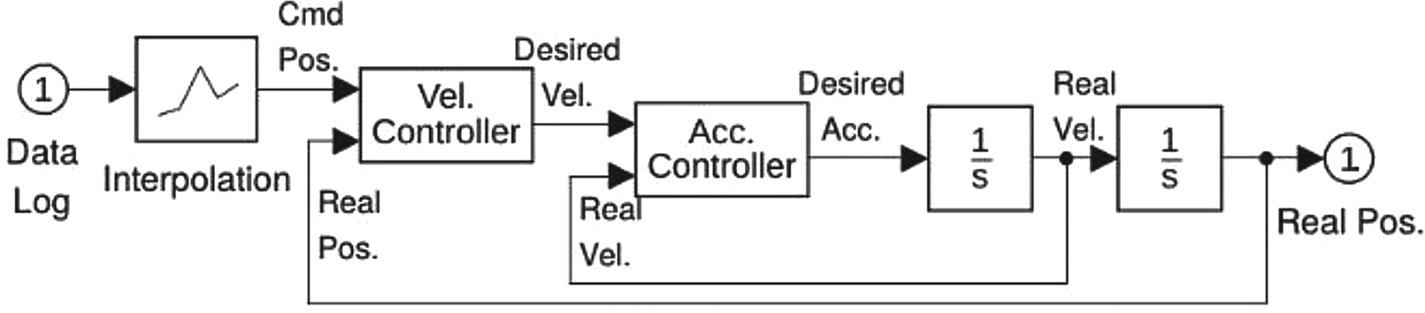
One way to generate a ‘good’ trajectory is to see the problem as a plant-control system. A simplified model of an aircraft is controlled on the interpolated flight path with eligible inputs (accelerations, velocities). The aircraft is simulated by a six degrees of freedom (6-DOF) decoupled model. Each DOF is considered individually using two integrators and is controlled by acceleration (Figure 3, middle). This method gives the flexibility to determine maximum velocity and acceleration for each DOF individually. The two-integrator model ensures continuity of position and velocities. The aircraft will pass flight log points only if they are reachable with logical acceleration and velocities. If noisy GPS data generates a highly rugged path, the aircraft will go through an averaged route among the points. This solution is not dependent on the number of points and spacing between them. It has the advantage of working with highly distant data-log points which gives the ability to design the path instead of collecting real flight data.
The plant-control system used for path tracking

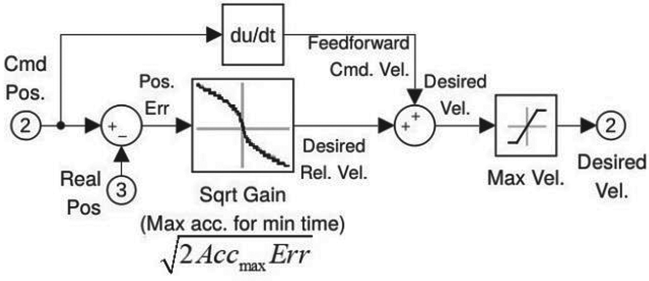
Two inner controller loops are used for each channel to keep the aircraft on course. Each loop uses a SQRT controller, inspired by a diagram in Copter Attitude Control (2016). Although not described in any paper, the SQRT controller is a useful, nonlinear, (near) minimum time controller. It is inspired by a car driving in traffic. A hurrying driver tries to reach the bumper of the car in front with maximum constant braking. It is selected as it allows one to reach the target with constrained acceleration and velocities and no overshoot. Constraining accelerations and velocities are derived from the object properties. SQRT gain gives the velocity derived from the well-known constant acceleration formula, Equation (1). In this formula, x 1 is the input error, v 1 is the desirable relative velocity to the target, x 2 is the position at the target (set to zero), v 2 is the relative speed at the target (also set to zero), and a max is the maximum allowed acceleration. This finally gives a square root form of the desired velocity with respect to the error known as SQRT gain, Equation (2).
 \begin{align}{v_2}^2 - {v_1}^2 &= 2{a_{\max }}({x_2} - {x_1})\end{align}
 \begin{align}v &= \sqrt {2{a_{\max }}x}\end{align}
Note that due to the infinite slope of the gain at the origin, this controller may chatter near the target. To overcome this problem, a small linear region is added to the centre. As this velocity is relative to the target, the final desired velocity is formed by simply adding target velocity (as a feed-forward). Velocity saturation is finally applied to constrain velocities (Figure 4).
The complete SQRT controller structure

Besides position and velocity, this controller can virtually be used for controlling any variable, by giving its desirable derivative. After getting the aircraft's position, angles and linear/rotational velocities, those for the camera are easily obtained. Assuming the aircraft's distance to objects is much larger than the distance between the aircraft's centre of mass and the camera position, the camera position is found:
 \begin{equation}\begin{aligned} {R_{\textrm{Cam}}}{|_{\textrm{NED}}} & ={R_{\textrm{AC}}}{|_{\textrm{NED}}} + {R_{\textrm{Cam/AC}}}{|_{\textrm{NED}}}\\ & ={R_{\textrm{AC}}}{|_{\textrm{NED}}} + C_{\textrm{AC}}^{\textrm{NED}}{R_{\textrm{Cam/AC}}}{|_{\textrm{AC}}} \approx {R_{\textrm{AC}}}{|_{\textrm{NED}}} \end{aligned}\end{equation}
Camera velocities (in camera coordinates) are also simplified and determined:
 \begin{equation}\begin{aligned} { {{V_{\textrm{Cam}}}} |_{\textrm{Cam}}} = { {{V_{\textrm{AC}}}} |_{\textrm{Cam}}} + {W_{\textrm{AC/NED}}} \times {R_{\textrm{Cam/AC}}}\\ \approx { {{V_{\textrm{AC}}}} |_{\textrm{Cam}}} = { {C_{\textrm{AC}}^{\textrm{Cam}}C_{\textrm{NED}}^{\textrm{AC}}{V_{\textrm{AC}}}} |_{\textrm{NED}}} \end{aligned}\end{equation}
Camera rotational velocity is determined in Equation (5). The camera is assumed to be fixed on the aircraft body.
 \begin{equation}\begin{aligned} { {{W_{\textrm{Cam/NED}}}} |_{\textrm{Cam}}} & ={ {{W_{\textrm{AC}}}} |_{\textrm{Cam}}} + { {{W_{\textrm{Cam/AC}}}} |_{\textrm{Cam}}}\\ & =C_{\textrm{AC}}^{\textrm{Cam}}{ {{W_{\textrm{AC/NED}}}} |_{\textrm{AC}}} + { {{W_{\textrm{Cam/AC}}}} |_{\textrm{Cam}}} \approx C_{\textrm{AC}}^{\textrm{Cam}}{ {{W_{\textrm{AC/NED}}}} |_{\textrm{AC}}} \end{aligned}\end{equation}
4. Ideal camera simulation
An ideal camera is usually interpreted as one with a pinhole camera model, as in Equation (6). An assumption of brightness constancy is also made for simplicity. This means that every point has the same brightness (and colour) when looked at from any angle.
 \begin{equation}\begin{aligned} & h \left( {\left[ {\begin{array}{*{20}{c}} x\\ y\\ z \end{array}} \right]} \right) = h\left( {\left[ {\begin{array}{*{20}{c}} u\\ v \end{array}} \right]} \right) = \left[ {\begin{array}{*{20}{c}} {{o_x}}\\ {{o_y}} \end{array}} \right] + \left[ {\begin{array}{*{20}{c}} {{f_x}} & 0 \\ 0 &{{f_y}} \end{array}} \right]\left[ {\begin{array}{*{20}{c}} u\\ v \end{array}} \right]\\ & \left( {u: = {{x \over z}},v: = {{y \over z}}} \right) \end{aligned}\end{equation}
In this equation, the final pixel location h is a function of a point's location in camera coordinates x, y, z. This location is first normalised to u, v values. The ideal pinhole camera model has the parameters fx, fy, ox and oy. These are the focal length and pixel shifts. For ideal camera simulation, a custom OpenSceneGraph (OpenSceneGraph Library, Reference Oettershagen, Stastny, Mantel, Melzer, Rudin, Gohl, Agamennoni, Alexis, Siegwart, Wettergreen and Barfoot1998) simulation is utilised. It consists of scenery and camera nodes.
To make a realistic camera frame, colour and depth information are needed. Without loss of generality, we use digital satellite imagery available online from Bing maps (2005)Footnote 4 and 1 arcsec digital elevation map from Farr et al. (Reference Farr, Rosen, Caro, Crippen, Duren, Hensley, Kobrick, Paller, Rodriguez and Roth2007) as geographic data samples in this work. Sample data are meant to be as real as possible, just to allow a comparison with real captured images.
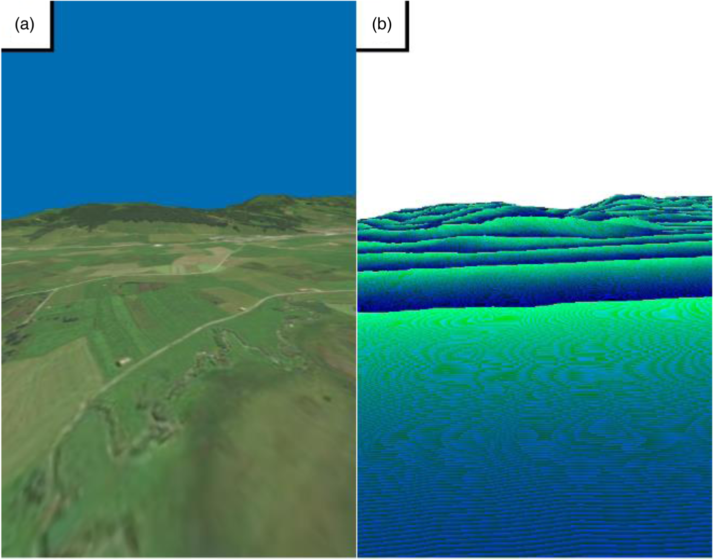
Two synchronised co-centred cameras are placed on the scene, using camera position and angle data generated by Equations (2)–(4). One camera gives a standard colour frame, while the other gives the depth frame. The depth camera has a modified shader to render distance of points to the camera plane (depth) instead of colours in full resolution (24 bits). This ideal full resolution depth and colour frames are later used in the distortion adding process. As adding geometrical distortions (like lens effect or rolling shutter) may need visual data from outside the final field of view (FOV), a bigger FOV (by a threshold) is rendered. These frame outputs are rendered in GPU but not shown, they are redirected to GPU memories (known as textures) for further processing (Figure 5).
Ideal and bigger rendered map of FSR 2015-ASL dataset, the first image in the lawnmower sequence: (a) colour rendering (b) 24 bit depth rendering. Notice that horizontal lines in depth map are blue channel (3rd byte) discontinuities

5. Geometric distortions simulation
Geometric distortions are deviations from the pinhole camera model caused by the lens. The most common lens distortion model used is the Brown five parameter model (Brown, Reference Brown1966), describing radial and tangential distortion in the pixels:
 \begin{equation}h\left( {\left[ {\begin{array}{*{20}{c}} u\\ v \end{array}} \right]} \right) = \left[ {\begin{array}{*{20}{c}} {{o_x}}\\ {{o_y}} \end{array}} \right] + \left[ {\begin{array}{*{20}{c}} {{f_x}}&0\\ 0&{{f_y}} \end{array}} \right]\left( {{d_r}\left[ {\begin{array}{*{20}{c}} u\\ v \end{array}} \right] + {d_t}} \right)\end{equation}
In this equation, radial and tangential distortions (dr and dt) are defined as:
 \begin{align} r&: = {u^2} + {v^2}\notag\\ {d_r}&: = (1 + {k_1}{r^2} + {k_2}{r^4} + {k_3}{r^6}) \end{align}
 \begin{align}{d_t}&: = \left[ \begin{array}{c} {2uv{p_1} + (r + 2{u^2}){p_2}}\\ {2uv{p_2} + (r + 2{v^2}){p_1}} \end{array} \right]\end{align}
Brown radial distortion parameters are k 1, k 2 and k 3 which together form the radial distortion dr. Brown tangential distortion parameters p 1 and p 2 form the tangential part dt. The biggest problem in utilising this model is that its inverse is required to model the distortion caused by the lens, in a fragment shader. Unfortunately, this model is known to have no closed-form inverse. Even for the radial only problem which is a degree 5 or 7 polynomial, the Abel-Ruffini theorem states that a finite general solution does not exist. The usual way to undistort or distort a sequence of images is to pre-compute the transformation map and then warp the image using this map (Bing maps, 2005; Rehder et al., Reference Shelley2016). Although it is fast, this is only possible if the distortion coefficients are fixed (i.e., zoom is fixed in-the-run or distortion coefficients remain constant while zooming).
To solve the problem online, an iterative Gauss–Newton inverse solution is used, like the one in Rehder et al. (Reference Shelley2016). It is simple enough to be run on a GPU fragment shader online. Although there is no proof of convergence, our experiments show that it generally works well in practice. Non-converged regions are rendered in red colour for clarity (as in Figures 11 and 12). These regions are usually caused by using inappropriate calibration patterns (e.g., see Figure 12). Notice that for a fixed-lens camera, the calculations are repeated in every frame and all the pixels remain converged if they have converged once. In the test case of a badly installed fisheye lens (Section 8.3), it converges in less than four iterations for all pixels within a 0⋅1-pixel accuracy.
6. Temporal distortion model
Temporal distortions are those that cause the displacement of pixels caused by ‘small’ timeshifts. Although named differently, image delay, motion blur, rolling shutter and interlacing are all caused by timeshifts and obey the same formulations.
Several works consider adding motion blur to still (ideal) images. This paper is limited to those that incorporate the depth of pixels (not consecutive frames) as an input. For exact timeshift modelling, one should render frames in every timeshift (e.g., every row for rolling shutter) and then mix them, which is a non-real-time solution. Rendering a frame in this way may take up to tens of seconds (Huang et al., Reference Huang, Hou, Ren and Zhou2012; Zhang et al., Reference Yu, Cai and Chen2014). An overview of motion blur generating methods is presented in Navarro et al. (Reference Mueller, Smith and Ghanem2011). In Atashgah and Malaek (Reference Atashgah and Malaek2013) and Zhao et al. (Reference Zhang, Wang, Sun and Han2014) a model is developed to simulate earth surface motion blur as a function of the aircraft's rotational and linear velocities and the focal length. These models assume the pixel travel as linear in every frame, which causes deformations in in-plane camera rotations (discussed in Section 8.4). Although it is not explicitly stated, the model in Atashgah and Malaek (Reference Atashgah and Malaek2013) seems to run online. In theory, rolling shutter and motion blur are both timeshifts and can be produced in the same way. A unified model for modelling motion blur and rolling shutter simultaneously was first introduced by Meilland et al. (Reference Mahmoudi2013). This model used mixing multiple renders to generate motion blur and was offline. In Guertin et al. (Reference Guertin, McGuire and Nowrouzezahrai2014) the problem of real-time motion blur is discussed along with the removal of artifacts over edges. In Gribel and Akenine-Möller (Reference Gribel and Akenine-Möller2017) interactions between ray-tracing and motion blur were discussed. None of these works consider the lens effect combined with general temporal distortions (delay, blur, rolling shutter and interlacing).
Exploiting the simulated depth of pixels, it is possible to develop a short-term time displacement model for every pixel. The model predicts source pixel displacements in the ideally rendered image. It utilises a single colour + depth frame and camera velocities. In this model, both linear and angular velocities are assumed to be fixed during the timeshift. Since the maximum rolling shutter and motion blur timeshift is in the order of tens of milliseconds, this seems acceptable, except at extreme linear-rotational accelerations. As image delay might be quite large (in the order of a tenth of a second), it is not recommended to model it by this model. Fixed image time delay can easily be added to the whole images by buffering the camera path.
Assuming small linear pixel-wise travel, the camera model is linearised to achieve a short-term displacement model:
 \begin{equation}\frac{{dh}}{{dt}}(u,v) = \frac{{\partial h}}{{\partial u}}\frac{{\partial u}}{{\partial t}} + \frac{{\partial h}}{{\partial v}}\frac{{\partial v}}{{\partial t}} = \frac{{\partial h}}{{\partial u}}\dot{u} + \frac{{\partial h}}{{\partial v}}\dot{v}\end{equation}
In this equation, time derivatives of normalised pixel coordinates are calculated as follows in Equations (11) and (12).
 \begin{equation}\begin{aligned} \dot{u} & =\dfrac{{\partial ({\raise0.5ex\hbox{$\scriptstyle x$}\kern-0.1em/\kern-0.15em\lower0.25ex\hbox{$\scriptstyle z$}})}}{{\partial t}} = \dfrac{{z\dot{x} - x\dot{z}}}{{{z^2}}} = \dfrac{{\dot{x}}}{z} - \dfrac{x}{z}\dfrac{{\dot{z}}}{z} = \dfrac{{{V_x}}}{z} - u\dfrac{{{V_z}}}{z}\\ \dot{v} & =\dfrac{{\partial ({\raise0.5ex\hbox{$\scriptstyle y$}\kern-0.1em/\kern-0.15em\lower0.25ex\hbox{$\scriptstyle z$}})}}{{\partial t}} = \dfrac{{{V_y}}}{z} - v\dfrac{{{V_z}}}{z} \end{aligned}\end{equation}
Note that z is pixel depth and is assumed to be constant during the time period. As all points are assumed to be stationary, point velocities in camera frame (Vx, Vy and Vz) are just a function of camera velocity and rotational speeds.
 \begin{equation}{ {{V_{\textrm{point/Cam}}}} |_{\textrm{Cam}}} ={-} { {{V_{\textrm{Cam/Inertia}}}} |_{\textrm{Cam}}} - { {{W_{\textrm{Cam}}}} |_{\textrm{Cam}}} \times { {{R_{\textrm{point}}}} |_{\textrm{Cam}}}\end{equation}
As the lens distortion (dr and dt) is already removed in the reverse pipeline, derivatives of h can be derived easily.
 \begin{equation}\frac{{\partial h}}{{\partial u}} = \left[ {\begin{array}{*{20}{c}} {{f_x}}\\ 0 \end{array}} \right],\textrm{ }\frac{{\partial h}}{{\partial v}} = \left[ {\begin{array}{*{20}{c}} 0\\ {{f_y}} \end{array}} \right]\end{equation}
It is interesting to note that the inverse temporal displacement model is independent of the distortion model. The final displacement caused by the time displacement is calculated as follows:
 \begin{equation}h(u(t),v(t)) \approx h(u({t_0}),v({t_0})) + \frac{{dh}}{{dt}}({u({t_0}),v({t_0}),{\raise0.7ex\hbox{${\vec{V}}$} \!\mathord{/ {\vphantom {{\vec{V}} z}} }\!\lower0.7ex\hbox{$z$}}({t_0})} )\Delta t\end{equation}
In Equation (14), V/z is the normalised velocity of a 3D point in and with respect to the camera coordinates. It is needed for calculation of u, v derivatives in Equation (11), and is assumed to be fixed during the small timeshift in the following equations. Equation (14) is simplified, for clarity, to Equation (15).
 \begin{equation}h(t) \approx h({t_0}) + \frac{{dh}}{{dt}}({{t_0}} )\Delta t\end{equation}
Note that the inverse is needed in the reverse pipeline to get from the known distorted coordinates h(t) to the undistorted coordinates h(t 0) in Equation (16).
 \begin{equation}h({t_0}) \approx h(t) - \frac{{dh}}{{dt}}({t_0})\Delta t \approx h(t) - \frac{{dh}}{{dt}}(t)\Delta t\end{equation}
This model is called the (inverse) linear displacement model. By redefining the derivative as negative, this equation finally becomes a standard differential equation.
 \begin{equation}\begin{split}
&h({t_0}) \approx h(t) + \dfrac{{d{h^ - }}}{{dt}}(t)\Delta
t\\ &\left( {\dfrac{{d{h^ - }}}{{dt}}: ={-}
\dfrac{{dh}}{{dt}}} \right)
\end{split}\end{equation}
Note that linearisation might cause some errors in case of high rotations, as seen in Figure 13. To improve the simulation's accuracy, one can implement a non-standard backward two-point Runge-Kutta order 2 (RK2) solver. The idea of RK2 is to use the average derivatives at the initial point and at the first estimate solution point. Based on this idea, the proposed solution is described in Equation (18).
 \begin{equation}\begin{split}
{h_1}({t_0}) & =h(t) + \dfrac{{d{h^ - }}}{{dt}}(t)\Delta
t\\ {h_2}({t_0}) & =h(t) + \dfrac{{(d{h^ - }/dt)(t) + (d{h^
- }/dt)({t_1},{h_1})}}{2}\Delta t
\end{split}\end{equation}
To further improve the RK2 accuracy, the t−t 0 timebase is divided into multiple time-steps and the solver is run multiple times (Figure 13).
6.1 Rolling shutter modelling
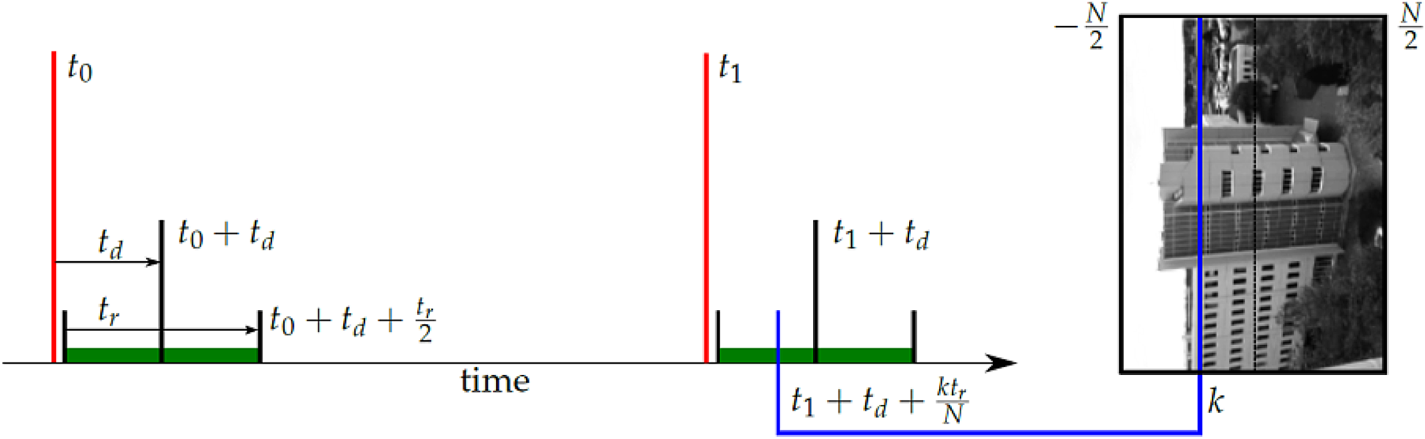
Rolling shutter cameras have a timeshift in subsequent image rows (or columns) (Figure 6). When an image is captured, a timestamp is provided (ti | i = 0, 1, 2 …). The middle row of the image was captured at some time ti + td. Notice that td is usually negative. The entire image of N rows has a read time of tr, meaning that row k was captured at ti + td + k.tr/N where  $k \in [{\textstyle{{ - N} \over 2}},{\textstyle{N \over 2}}]$ (Shelley, Reference Shah, Dey, Lovett and Kapoor2014). The timeshift is thus assumed to be
 \begin{equation}\Delta t = t - {t_i} = {t_d} + k\frac{{{t_r}}}{N}\end{equation}
Timeshift caused by rolling shutter

The final h is the one without the lens and rolling shutter distortions, so its colour and depth can be read easily from the ideal image rendered earlier.
6.2 Motion blur modelling
For modelling motion blur, an exposure time of te is considered for each pixel in each image. Using the displacement model, two sample pixel positions (h points) using the beginning and end of this exposure time are generated.
 \begin{equation}\begin{split}
\Delta {t_1} & ={t_d} + k\dfrac{{{t_r}}}{N} -
\dfrac{{{t_e}}}{2}\\ \Delta {t_2} &
={t_d} + k\dfrac{{{t_r}}}{N} + \dfrac{{{t_e}}}{2}
\end{split}\end{equation}
These points form a sampling line in the ideally rendered frame. Colours on this sampling line are averaged to form the final colour caused by motion blur.
6.3 Interlacing
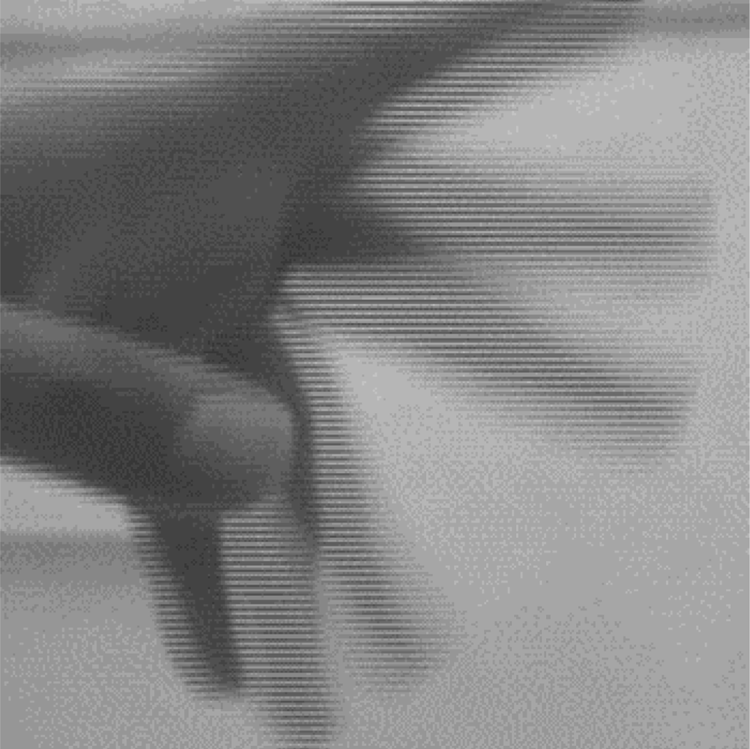
For better visual feeling, analog videos come in double frequencies and half rows. At the time of visualisation (or in the analog to digital device), two consecutive odd and even frames are mixed to construct a full frame (Figure 7). Interlacing can cause serious problems in image processing, much worse than rolling shutter. This operation is reversible only if no image loss due to compression occurs in the analog to digital device, otherwise a wavy image on the edge of moving parts is generated. The timeshift model for the interlacing is demonstrated in Equation (21).
 \begin{equation}\Delta t = {t_d} + k\frac{{{t_r}}}{N} \pm \frac{{{t_e}}}{2} - \frac{{k\%2}}{{2fps}}\end{equation}
Interlacing combines two consequent half-row frames like a zipper, to form a full-frame one

7. Photometric distortion simulation
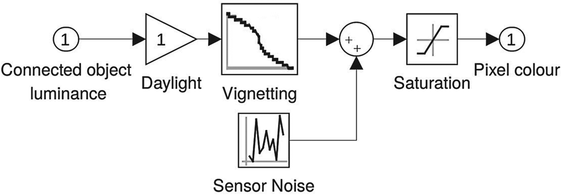
Photometric distortions cause changes in pixel brightness. They are static (e.g., vignetting) or dynamic (noise, light level etc.). These imperfections are implemented for each output pixel after geometrical distortions. As they are independent, they are easily parallelised (in the pixel-wise fragment shader).
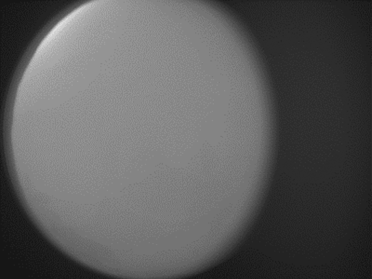
Vignetting is the reduction of the image's brightness or total saturation towards the edges of the frame. A vignetting frame is obtained by taking a picture from a white wall in full light (Figure 8). It is sent to the GPU shader, thresholded to eliminate noise in central image areas and finally multiplied by the brightness of pixels in the shader.
Vignetting map of a badly installed fisheye lens on Galaxy S3 main camera

Although simple shadowing/ray-tracing methods exist, they interfere with the existing shadows/light gradient on the satellite images. In this study, the light source, the reflectance of light, and shades as they already exist are ignored. The environment light level is just modelled by a gain. An additive Gaussian sensor noise is also implemented. Finally, saturation is used to keep the pixel values in the 0 to 1 range (Figure 9).
Pixel-wise photometric model, including vignetting, colour noise, light level and saturation

8. Results, test and evaluation
8.1 Tracking performance
The flight log data in the FSR 2015 ASL, lawnmower sequence, is used as the test case. Tracking performance is determined by the root mean squared (RMS) distance of tracker output from the interpolated values of the flight log. Maximum accelerations in linear and angular channels are assumed to be 2 g and 60 deg/s2 (Table 1). Notice that as the data in the flight log has noise, it is natural that the generated flight path with real acceleration and velocity constraints is closer to reality.
Flight log tracking RMS error

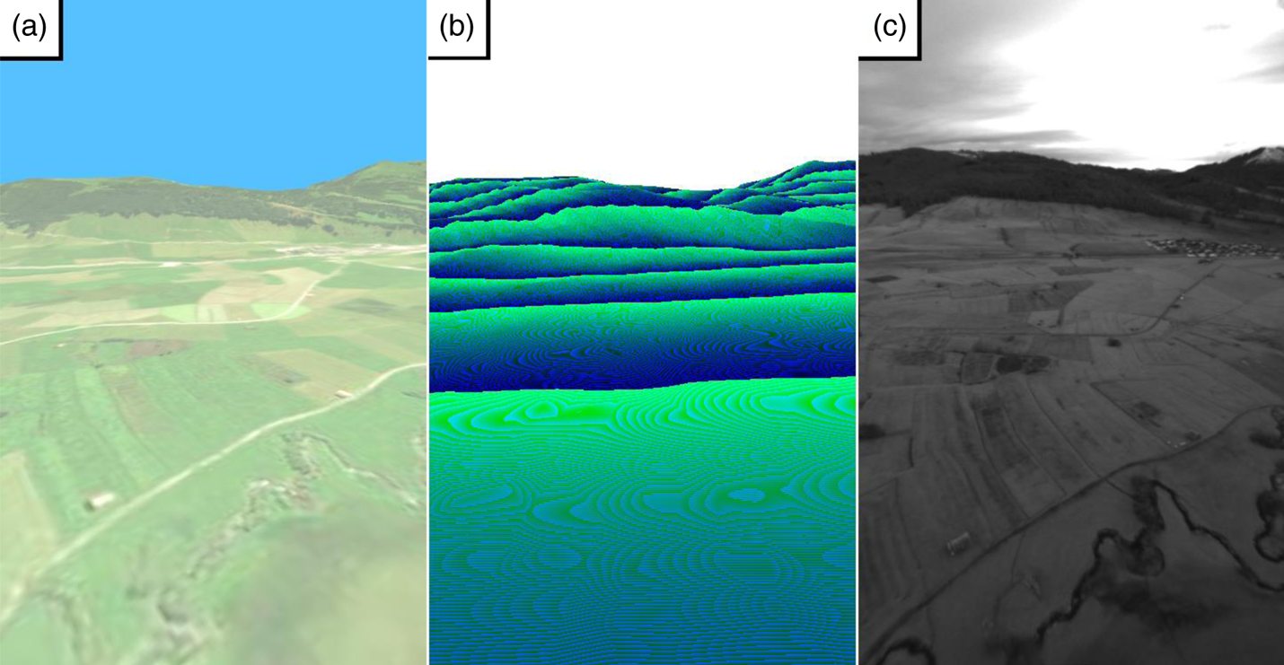
8.2 Ideal camera rendering test
Snapshots from the simulation output can be seen in Figure 10. They include light intensity images along with depth-maps generated from camera FOV. Although exact earth simulation is not the main focus of this work, its validation can show the correctness of the ideal (pinhole) camera model and its placement. The first frame of the oblique grey camera present in the lawnmower sequence is used as the test case. As lens distortion simulation is not meant in this test, the distortion is eliminated from the captured image using standard routines. Eight manually selected corresponding points are selected in the simulated and real images. Using the well-known eight-point algorithm (Hartley, Reference Hartley1997), the rotation between two images is shown to be about 6 degrees, which can be due to errors in the flight log and IMU installation, or in the elevation map and orthographic images.
Simulation of FSR 2015-ASL dataset, the first image in the lawnmower sequence: (a) final simulator output, (b) 24 bit depth, (c) undistorted captured image

8.3 Lens model test
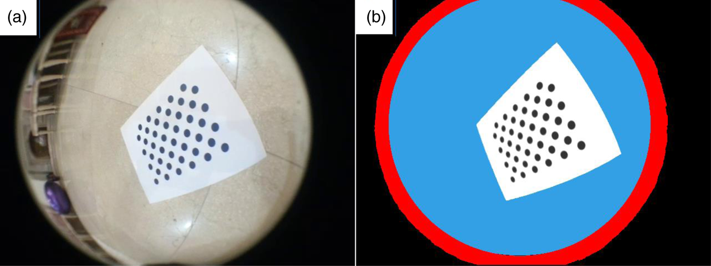
For testing lens simulation accuracy, a test procedure is designed. OpenCV uses various calibration patterns for lens modelling. One of them is the asymmetric circular pattern (Figure 11). By taking multiple (60) 640 × 480 photographs of this calibration pattern from different angles, a standard OpenCV routine can be usedFootnote 5 to determine both intrinsic (calibration) and extrinsic (positioning) parameters of this camera. These calibration and positioning data are fed into the simulation along with a vignetting map, as discussed in Section 7, to generate 60 simulated images of the calibration pattern.
(a) One of the 60 pictures taken from OpenCV's asymmetric circular calibration pattern, (b) simulation output

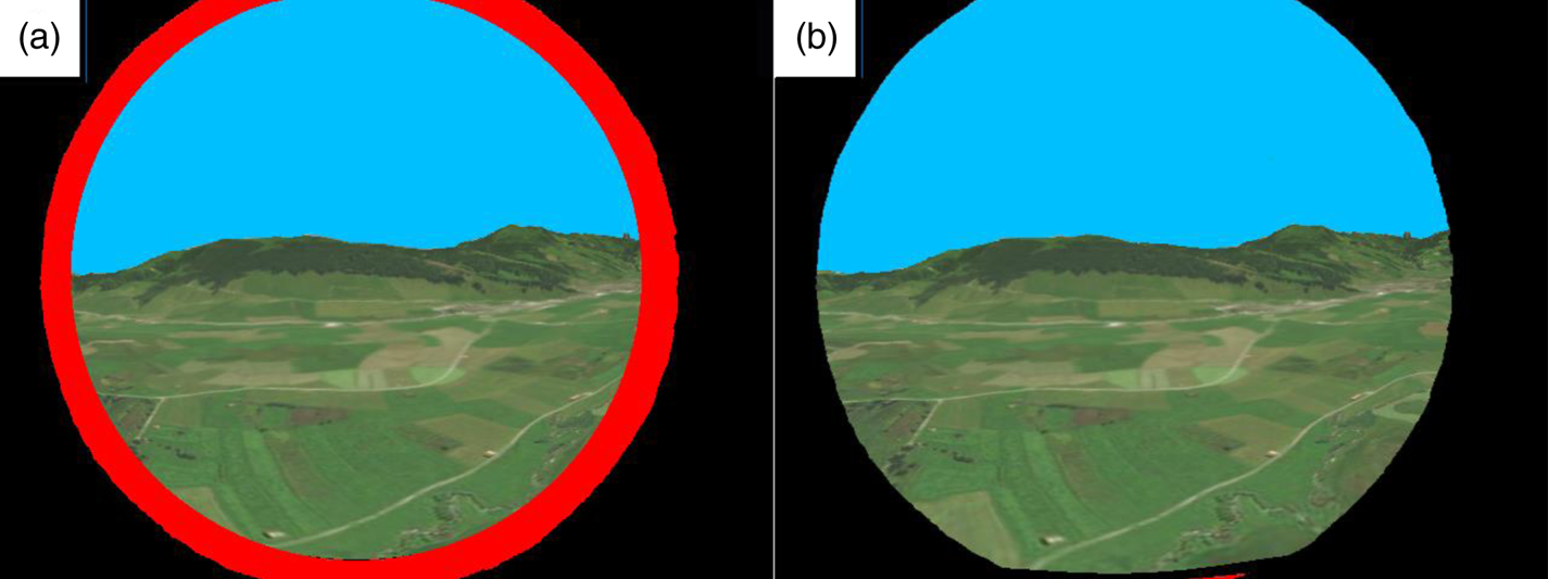
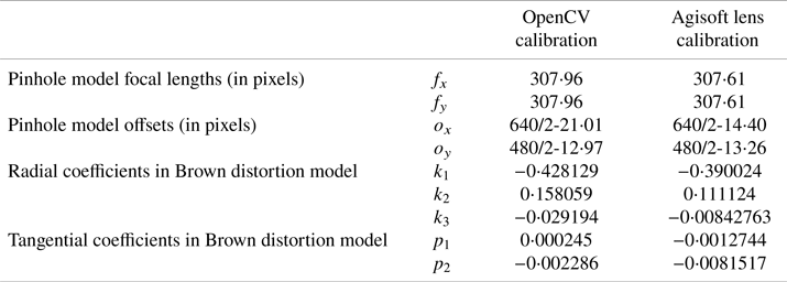
Termination criteria used for the iterative inverse algorithm are 0⋅1 pixels maximum error or a maximum of 50 iterations. A comparison routine compares the positions of the centre of the area of circles in all 60 real and simulated images.Footnote 6 It is found to have an RMS error of 0⋅73 pixels, which seems acceptable. Notice the red ring around the edge of the simulated frame. In this region, the lens inverse solver is not converged within predefined accuracy (0⋅1 pixels). This is because the pattern becomes highly distorted and undetectable at the frame edges, so the calibration algorithm does not give good results at the edges. By using the wide calibration pattern and algorithm provided by Agisoft Lens, this problem can be solved (Figure 12). Frame dimensions, ideal (pinhole) camera parameters, lens distortion parameters and solver parameters are presented in Table 2. The Agisoft parameters are used in the proceeding sections.
Simulation output using (a) OpenCV, (b) Agisoft Lens calibration parameters

Intrinsic ideal camera and lens distortion calibration parameters

8.4 Time displacement model test
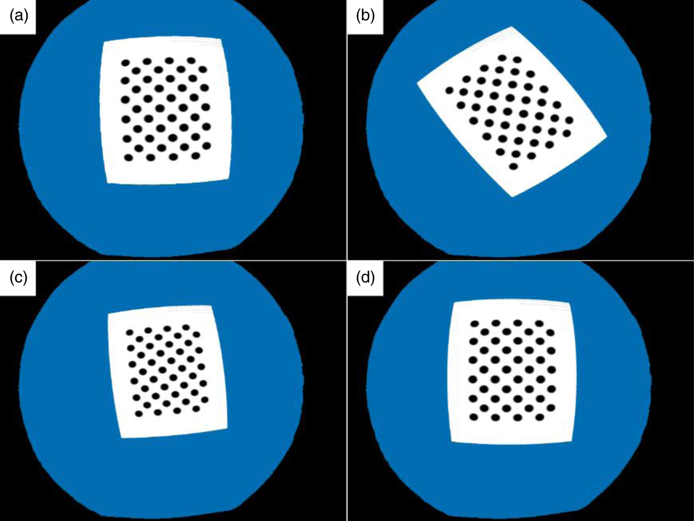
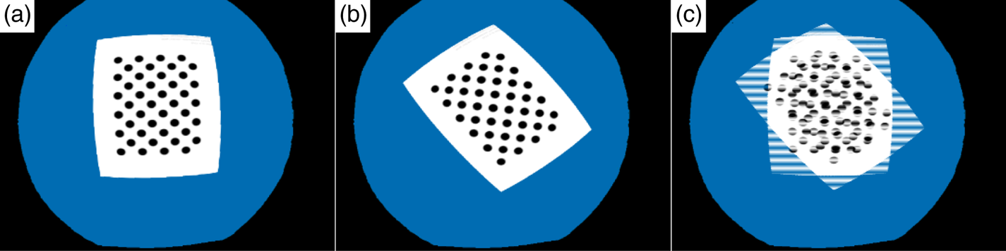
At the heart of temporal distortions, the time displacement model exists. If it is modelled correctly, time delay, rolling shutter, motion blur and interlacing models are mostly evaluated, too. We can do this evaluation by modelling delays in two separate rotational and translational motions. As shown in Figure 13, even a high amount of rotation (~36 degrees) is recovered correctly.
Delay effect under camera rotation: (a) original positioning, (b) pattern after 1 s of rotation (36 degrees), (c) 1 s rotation + 1 s delay using single-step linear solution, (d) using single-step backward RK2 solution

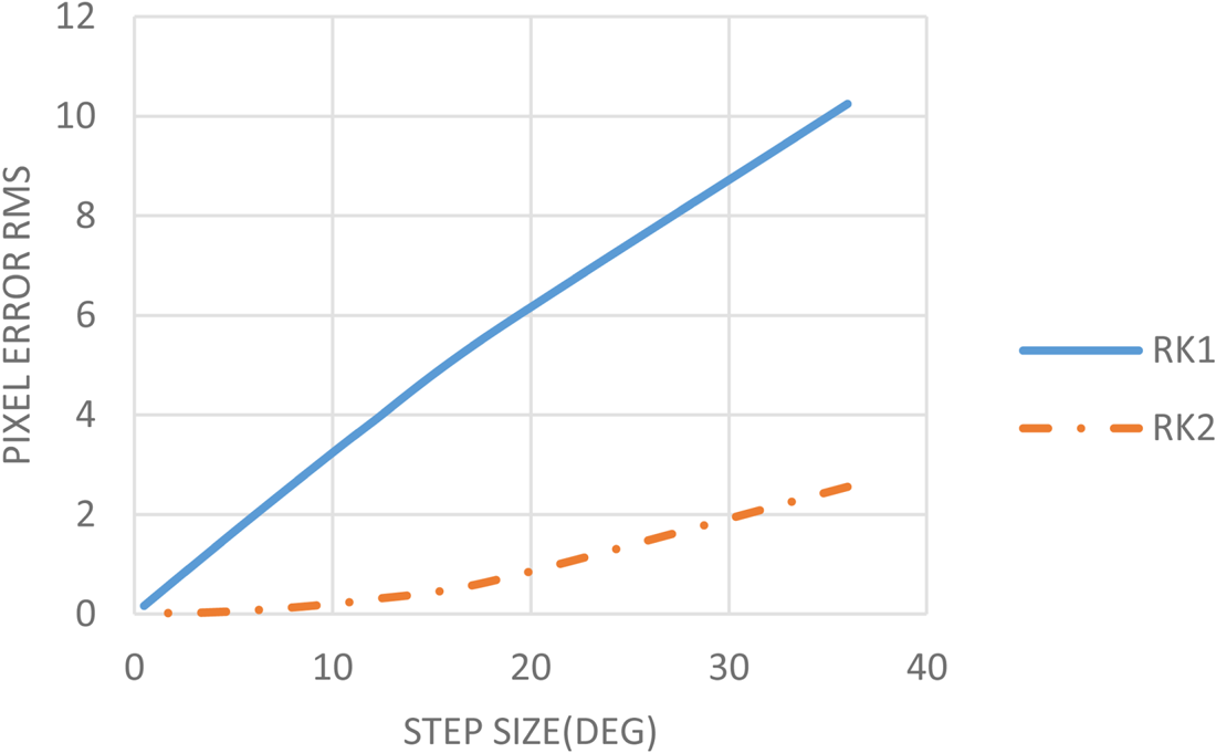
The accuracy of the model depends on the solver type, as discussed in Section 6, step size and the total amount of rotation. This is illustrated in Figure 14. The lower the step size or total amount of rotation, the better is the accuracy. This relation is almost linear. Notice the great effect of the solver type. RK2 solver doubles the evaluation points but increases the accuracy multiple times. The accuracy seems not to change much below 2⋅5 degrees of step size, giving an RMS error of 0⋅02 pixels. So this step size is considered as optimal.
Pixel error RMS versus step size for different solver types, total pattern rotation is 36 degrees between frames, validated step sizes are 36, 18, 12, 9, 6, 4, 3, 2, 1 and 0⋅5 degrees

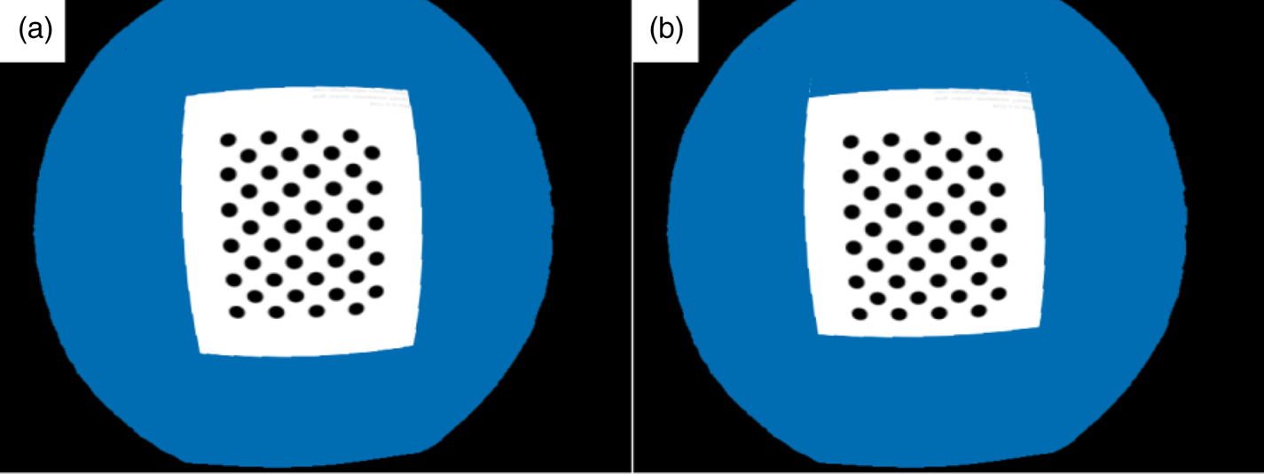
The delay effect in camera motion is linear in nature and accurately created even by a single-step linear solver (Figure 15). However, some problems might be seen at depth discontinuities like the bottom part of the pattern which disappears at its edge. This is due to the unsatisfied assumption of no depth change under small timeshift, which is not a significant problem in continuous terrains.
Delay effect under camera motion: (a) no delay (b) 1 s move + 1 s delay

8.5 Motion blur model test
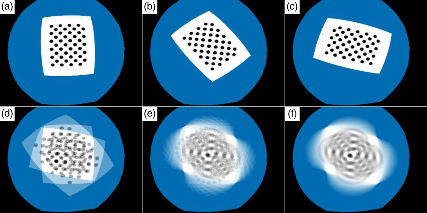
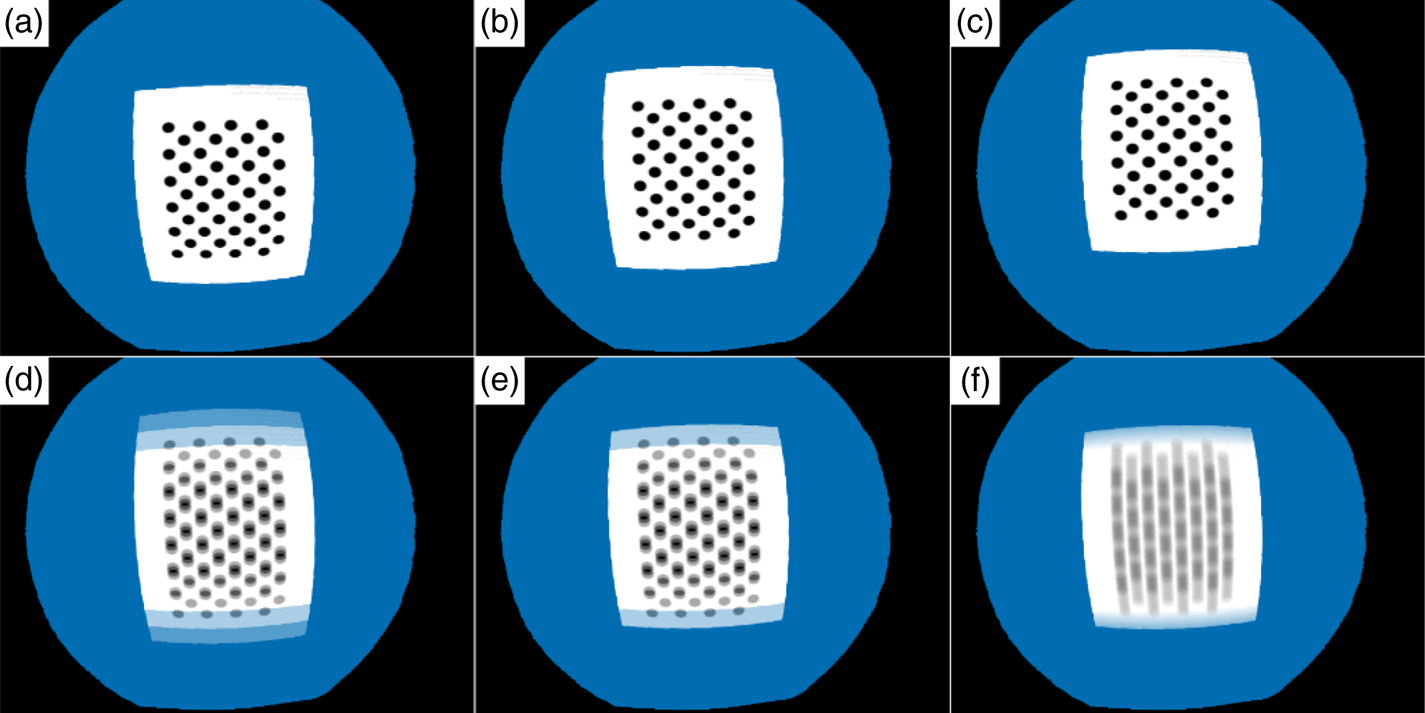
Motion blur can easily be evaluated by comparing it with overlaid delayed images (Figure 16). It can be seen that simulation output with three samples closely follows the overlay of three subsequent images. Simulation output becomes closer to the anticipated reality as the sample points increase. Motion blur under camera motion is also exactly modelled like the motion displacement model except at the edges (Figure 17).
Motion blur under camera rotation (a)–(c) static camera in three consequent positions (36 degree spacing), (d) simulation output using three sample points, (e) 10 sample points, (f) 100 sample points

Motion blur under camera motion: (a)–(c) static camera in three positions, (d) overlay of static images, (e) simulation output using three sample points, (f) simulation output using 100 sample points

8.6 Rolling shutter model test
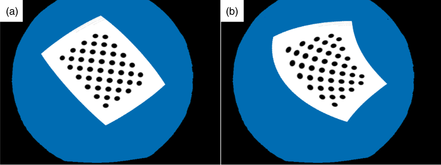
Motion blur is evaluated qualitatively. The rotation effect on the rolling shutter is demonstrated in Figure 18. The camera is rotating clockwise (CW), so the image rotates counter clockwise (CCW). The top rows are simulated as captured sooner, so they are rotated less CCW. The bottom rows are rotated more CCW.
Rolling shutter under camera rotation: (a) static camera, (b) camera rotating CW

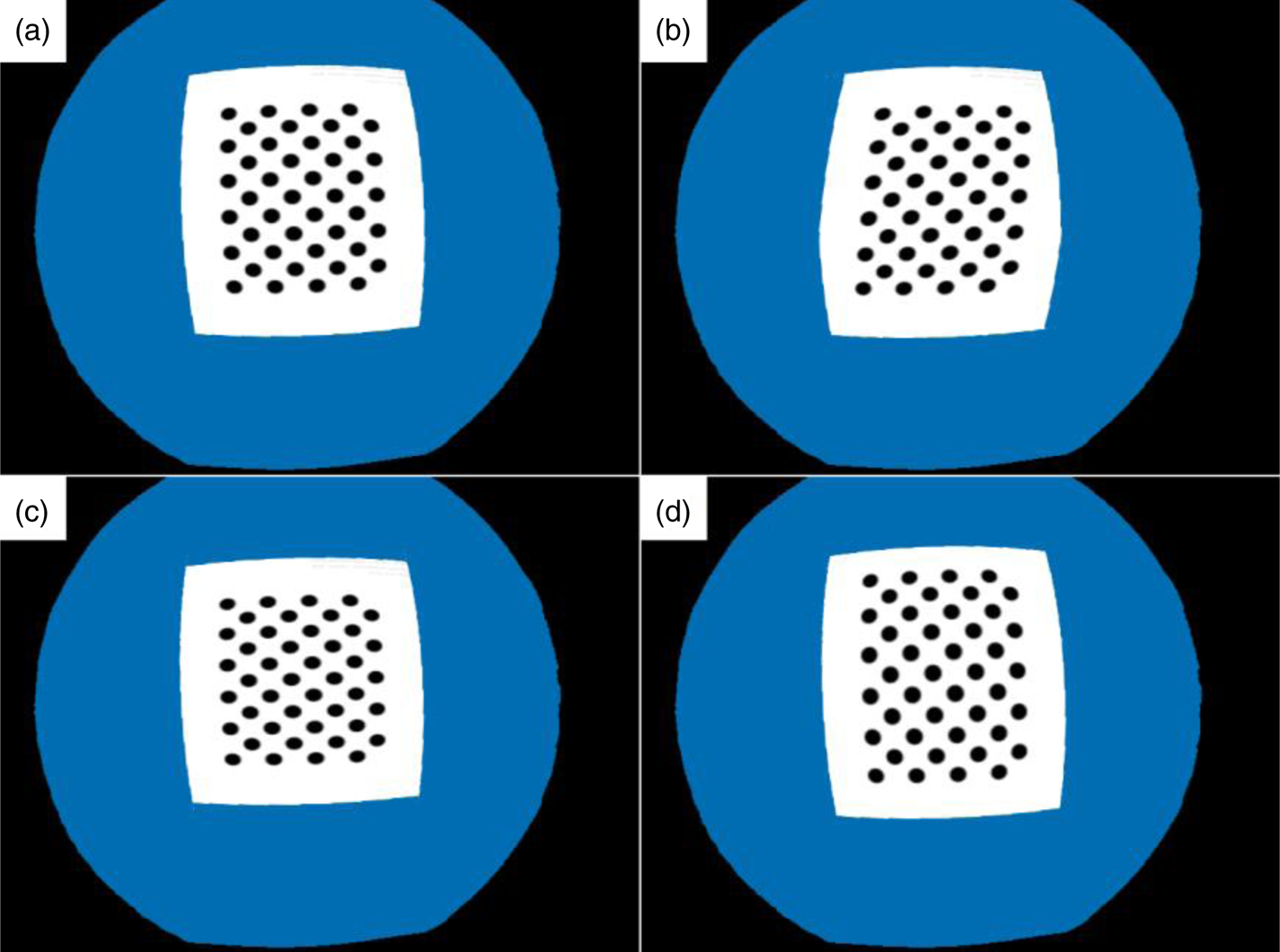
Under camera motion, the rolling shutter creates weird effects. Shearing, shortening and elongation are seen in Figure 19. Edge artifacts are still seen in the left of shear in Figure 19(b) and top of elongation in Figure 19(d).
Rolling shutter under camera motion: (a) static camera, (b) camera moving to the right (shear), (c) camera moving upwards (shortening), (d) camera moving downwards (elongation)

8.7 Interlacing model test
As seen in Figure 20, the interlacing effect is much like the motion blur with two sample points and can be evaluated the same way by comparing image overlays. The only difference is that, unlike motion blur, the delay is switching in odd and even rows.
Interlacing under camera rotation: (a) and (b) static camera in two positions, (c) simulated interlaced image at the second position

8.8 Time displacement on map
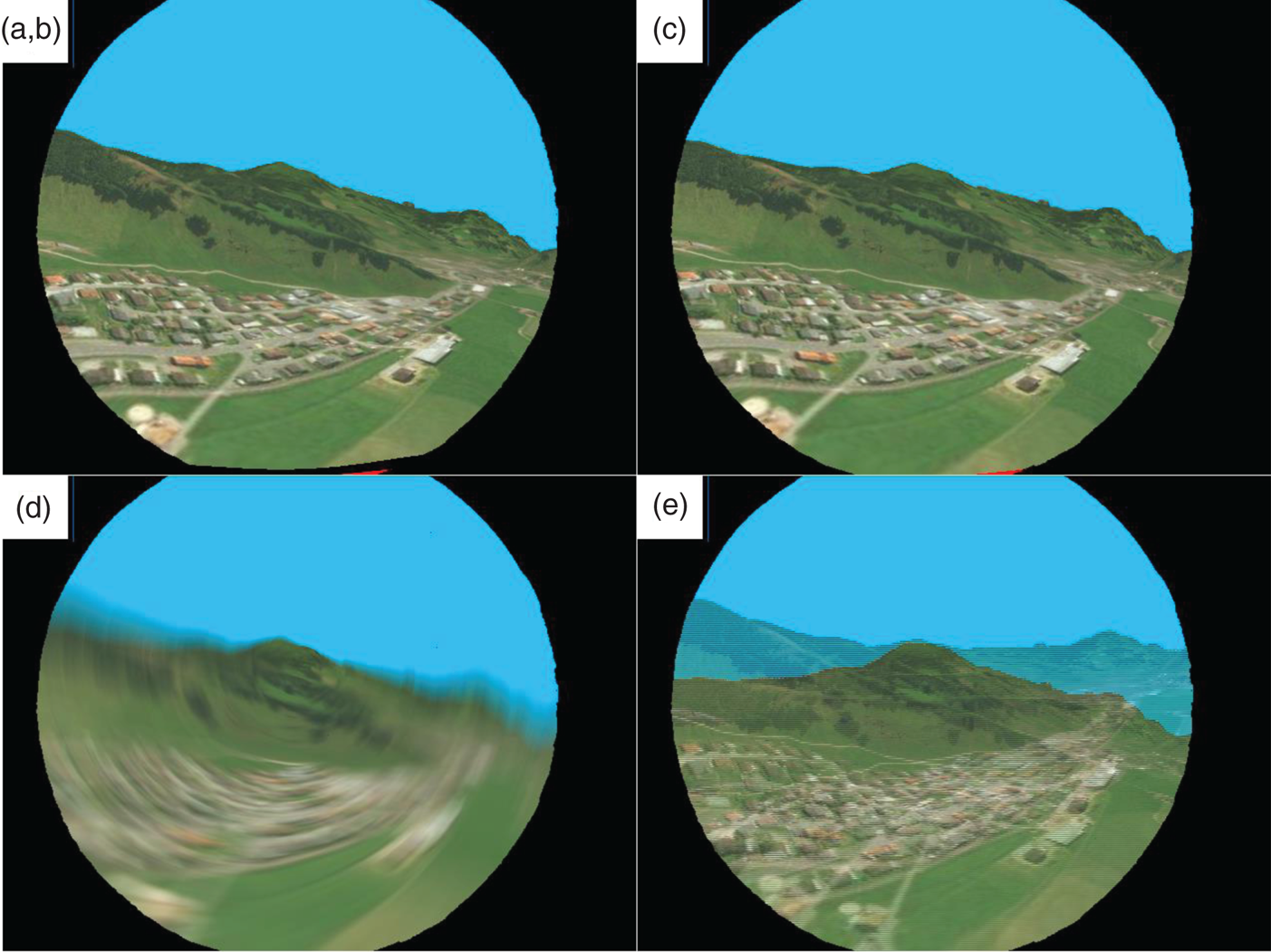
A video frame with a 640 × 480 dimension is generated on the lawnmower sequence in Figure 21(a). The camera's view is assumed to be exactly parallel to the nose of the aircraft. The aircraft/camera is rotating CCW and to the left. For visualisation purposes, all the distortion parameters are set with large values. A fisheye lens with high distortion levels is used (Table 2). All the time constants are exaggerated to 1 s, see Figure 21(b)–(e). In Figure 21(b) a 1 s delay is simulated, compensated by a 1 s timeshift. In Figure 21(c) rolling shutter is exaggerated. The up row belongs to half a second sooner and the down row half a second later. The image is shortened in the left and elongated in right as expected. Exposure time of 1 s causes extreme motion blur as expected, see Figure 21(d). Pure interlacing creates a two-fold image, see Figure 21(e). Notice that individual even and odd rows belong to different timestamps with 1 s spacing.
640 × 480 fisheye camera frame added to FSR 2015-ASL dataset, using exaggerated temporal distortions: (a) no temporal distortions, (b) 1 s later +1 s delay (visually indistinguishable from (a)), (c) 1 s rolling shutter (tr) (d) 1 s exposure time (te), (e) 1 s spacing for interlacing (ti)

8.9 Overall speed test
A typical core i7-7500 U CPU at 2⋅7 GHz with GeForce940MX GPU hardware was used during the experiment. With 100 blur sampling points, the frequency of the image generation algorithm exceeds 33 fps (frames per second) which surpasses a 30 fps camera. Having acceptable speed, using this as a real-time simulation framework needs further work as some jitter (hiccups) is seen in the timing of the output, in the order of hundreds of milliseconds.
9. Discussion and conclusion
This work has developed and evaluated a framework suitable for airborne RGB-D camera simulation. First, an eligible flight path is generated based on the flight log. Based on this path, an ideal pinhole RGB-D camera capable of rendering the earth's surface or a calibration pattern is developed. Camera model artifacts are added in a post-processing stage, in a GPU fragment shader. This is done by a reverse pipeline connecting each pixel in the output image to pixels in the ideally rendered input frame. Modelled artifacts are lens distortion, zoom changes, image delay, rolling shutter, motion blur, interlacing, vignetting, image noise and low light. This is the first work to combine the static (lens) and temporal distortions together in an online fashion. Previously even temporal distortions were not treated in an online unified framework. The developed shader program is published in a public repository (Mahmoudi, Reference Koenig and Howard2020) to make further development/usage possible.
As just an orthographic map was available to the authors for light intensity and colour modelling, nonlinear light intensity effects under different view angles and light conditions are not modelled. Using shadowing/ray-tracing methods could interfere with existing shadows/light gradient on the map and is not modelled. For elevation modelling, just a limited resolution digital elevation map was used, so it is assumed that high-frequency altitude clutter like buildings, jungle, sea waves and moving objects are not present in the view or the altitude is high enough to discard them. Further developments can include using an advanced off-the-shelf simulator before the provided post-processing shader to address these shortcomings.
Another assumption is that the linear-rotational speed of the camera does not change during the frame generation timebase (in the order of several milliseconds). This assumption might be simplistic in the presence of high-frequency vibrations. It is also assumed that the distance of the objects from the camera plane do not change in the timebase. This could cause infidelities in the temporal model in hybrid rotational and translational motions, especially on nearby objects with a high view angle. Another assumption is that pixel depths do not change due to linear camera motion, after timeshifts caused by delay, rolling shutter, exposure time and interlacing. This problem is already treated for pure motion blur in Guertin et al. (Reference Guertin, McGuire and Nowrouzezahrai2014). This might cause artifacts on the edges of nearby terrain discontinuities and could be tackled in a further paper.
Supplementary data
The complete simulator code is open sourced at: https://github.com/mah92/camsim.
Competing interests
The authors declare that there are no conflicts of interest regarding the publication of this paper.
Acknowledgements
This research did not receive any specific grant from funding agencies in the public, commercial, or not-for-profit sectors. Arshiya Mahmoudi would like to thank their instructors and family who understood the importance of the subject and provided enough time for the work to become mature. Special thanks to Imam Hussein for his mental support, especially during hard programming locks. The authors also thank the developers of the ‘Nasir framework’ project, making hybrid Android + Linux and OpenGL shader programming a lot easier.