1 Introduction
Synthetic jets have attracted a considerable amount of research over the past decades (e.g. Smith & Glezer Reference Smith and Glezer1998, Glezer & Amitay Reference Glezer and Amitay2002, Cattafesta & Sheplak Reference Cattafesta and Sheplak2011). The distinctive feature of synthetic jet actuators is the creation of a zero-net-mass-flux jet which has non-zero net momentum flux. These jets consist of alternating blowing and suction cycles through an orifice and are formed entirely from the working fluid. During the suction phase surrounding fluid is ingested into the actuator. The blowing phase is often modelled as a slug of fluid being ejected by the actuator. Part of this fluid slug rolls up into a vortical structure around the edge of the jet exit. This structure propagates away from the actuator, driven by a combination of its self-induced velocity and the momentum created by the jet. Since this jet is created from the working fluid, synthetic jet actuators do not require a fluid supply, making them practical to integrate in a range of flow-control applications. Synthetic jets in cross-flow can be used in a wide range of applications such as mixing enhancement (M’Closkey et al. Reference M’Closkey, King, Cortelezzi and Karagozian2002; Sau & Mahesh Reference Sau and Mahesh2008), control of turbulence (Rathnasingham & Breuer Reference Rathnasingham and Breuer2003) or separation control (Dandois, Garnier & Sagaut Reference Dandois, Garnier and Sagaut2007). In the present study the interaction of a synthetic jet with a turbulent boundary layer is considered where the jet is issuing in the direction normal to the bulk flow (i.e. in the wall-normal direction).
The interaction of a synthetic jet with a cross-flow can be compared to the canonical cases of steady jets in cross-flow (see for example the review by Mahesh Reference Mahesh2013) and forced jets in cross-flow (see for example the review by Karagozian Reference Karagozian2014). The present study focusses on the wake created by the jet in the cross-flow. This wake is of importance for most flow-control applications since it decreases the momentum and therewith potentially the (energy) efficiency of the control mechanism. An example is the recent investigation on reducing skin-friction drag in a high-Reynolds-number turbulent boundary layer through control of large-scale structures by Abbassi et al. (Reference Abbassi, Baars, Hutchins and Marusic2017). This study reports skin-friction drag reductions of up to 3.2 %. Skin-friction control in this case is obtained using a pulsed jet issuing from the surface through a rectangular slot oriented with the long dimension in the streamwise direction. If this were to be applied in an internal flow (for example a pipeline), any energy savings coming from the skin-friction reduction would be offset by the pressure loss caused by the emergence of a strong wake created by the pulsed jet. It is assumed that the wakes created by pulsed jets and synthetic jets are driven by the same mechanisms, discussed in the present study.
The interaction of a steady jet with a cross-flow, i.e. transverse jet, is a canonical case and the wake and its structure have been studied for decades (e.g. Kamotani & Greber Reference Kamotani and Greber1972; Broadwell & Breidenthal Reference Broadwell and Breidenthal1984; Fric & Roshko Reference Fric and Roshko1994). This interaction shares some features with the interaction of a synthetic jet with a cross-flow, such as blockage of the cross-flow by ejected fluid as well as the generation of vortical structures. Fluid ejected by the jet causes viscous blockage of the cross-flow. In the past this blockage has been compared to the wake behind a bluff body. The momentum deficit behind a wall-mounted bluff body is caused by momentum transfer of the flow to this body, which is subsequently transferred to the wall. Due to the lack of a rigid connection, such a transfer of momentum away from the flow is not possible for a jet in cross-flow (Fric & Roshko Reference Fric and Roshko1994; Morton & Ibbetson Reference Morton and Ibbetson1996). This does not imply there is no blockage wake in a jet in cross-flow: initially the fluid of the jet has zero streamwise momentum (relating to the direction of the cross-flow) and thereby blocks the cross-flow. This causes a transfer of streamwise momentum from the cross-flow to the ejected fluid, similar to the momentum transfer to a bluff body. Instead of transferring this momentum to the wall the jet fluid retains this momentum, leading to an acceleration in streamwise direction. The blockage and transfer of momentum continues until the ejected fluid reaches the same velocity as the surrounding cross-flow, which leads to a finite blockage wake downstream of the jet.
The transverse jet creates multiple types of coherent (vortical) structures (Fric & Roshko Reference Fric and Roshko1994). Two types are present in the mean flow; a horseshoe vortex around the base of the jet and a counter-rotating vortex pair aligned with the jet. The vortex pair, which induces an upward flow at the jet centre-plane lifts up low-momentum fluid from near the wall, causing a momentum deficit and apparent wake in the cross-flow (Fric & Roshko Reference Fric and Roshko1994; Kelso, Lim & Perry Reference Kelso, Lim and Perry1996; Morton & Ibbetson Reference Morton and Ibbetson1996; Cortelezzi & Karagozian Reference Cortelezzi and Karagozian2001). In addition to the blockage effect discussed above, this up-wash of low-momentum fluid is a second source of momentum deficit downstream of the transverse jet.
When forcing a jet, vortical structures are formed with the forcing frequency (Wu, Vakili & Yu Reference Wu, Vakili and Yu1988). Depending on the forcing parameters these vortical structures can form distinct vortex rings that may bifurcate from the core of the jet and can have a significantly larger wall-normal penetration in the cross-flow (Eroglu & Breidenthal Reference Eroglu and Breidenthal2001; Johari Reference Johari2006; Shapiro et al. Reference Shapiro, King, M’Closkey and Karagozian2006). The creation of vortex rings in a shear flow leads to a tilting of these rings with their axes in a slight opposite direction to the cross-flow (Lim, Lua & Thet Reference Lim, Lua and Thet2008; Cheng, Lou & Lim Reference Cheng, Lou and Lim2009). This means that (when subtracting their advection velocity) these rings have a slight self-induced motion in the direction opposite to the cross-flow. In addition they induce a velocity in the surrounding flow in the direction opposite to the cross-flow, resulting in a third source of momentum deficit downstream of the forced transverse jet.
The synthetic jet shares a lot of similarities with steady and forced jets. In fact, the velocity cycle at the orifice of all three (when using sinusoidal forcing) can be generalized as
 $$\begin{eqnarray}u_{j}(t)=\langle u_{j}\rangle +u_{j}^{\prime }\sin (2\unicode[STIX]{x03C0}tf),\end{eqnarray}$$
where
 $\langle u_{j}\rangle$
represents the time-averaged jet velocity and
 $u_{j}^{\prime }$
the amplitude of cyclic fluctuations of frequency
 $f$
around this average. For steady jets
 $u_{j}^{\prime }=0$
while for synthetic jets
 $\langle u_{j}\rangle =0$
. Forced jets consist of both a steady and a fluctuating component and can be considered to be an intermediary case between the steady and synthetic jet cases. As discussed above, when going from a steady to a forced jet the vortical structures created by the jet get locked onto the specified frequency
 $f$
. When moving to a synthetic jet, under certain conditions all of the jet fluid rolls up into vortices and the jet forms a train of vortical structures with the specified frequency (Smith & Glezer Reference Smith and Glezer1998). These vortical structures can be linked to all three sources of the momentum deficit discussed above; (I) they initially block the cross-flow, leading to a momentum transfer from the cross-flow to these structures, causing a momentum deficit in the flow downstream of the jet and accelerating the structures until they reach the velocity of the surrounding flow (Lardeau & Leschziner Reference Lardeau and Leschziner2011), (II) the vortical structures induce a velocity away from the wall at the centreline of the jet, causing up-wash of low-momentum fluid causing a momentum deficit away from the wall (Rathnasingham & Breuer Reference Rathnasingham and Breuer2003) and (III) the tilted vortical structures induce a velocity in the direction opposite to the cross-flow, causing a momentum deficit. This study focusses on the third source of momentum deficit: the velocity induced by vortical structures. Furthermore, it will be reasoned that the effects of blockage and up-wash on the momentum deficit are limited. The total momentum deficit is a combination of all three (and possibly other) factors. The ratio of the contributions of these effects will vary with downstream distance and depends on the flow parameters and the type of vortical structures created by the synthetic jet.
The velocity cycle of a synthetic jet as given by (1.1) (for
 $\langle u_{j}\rangle =0$
) can be characterized using a frequency
 $f$
and velocity magnitude
 $\bar{u}_{j}$
(Glezer & Amitay Reference Glezer and Amitay2002). The velocity magnitude used here is the mean blowing velocity, calculated as
 $\bar{u}_{j}=1/T\int _{0}^{T/2}u_{j}(t)\,\text{d}t$
, which is related to the amplitude by
 $\bar{u}_{j}=u_{j}^{\prime }/\unicode[STIX]{x03C0}$
. Alternative representative velocities are used throughout the literature, most notably the momentum flow velocity,
 $U_{0}~(\text{m}~\text{s}^{-1})$
, as defined by Cater & Soria (Reference Cater and Soria2002), relating to the mean blowing velocity as
 $U_{0}=\bar{u}_{j}\unicode[STIX]{x03C0}/\sqrt{2}$
. The velocity of the jet is normalized using the free-stream velocity,
 $U_{\infty }$
, resulting in a velocity ratio, given by
 $$\begin{eqnarray}r=\frac{\bar{u}_{j}}{U_{\infty }}.\end{eqnarray}$$
The frequency of the jet is normalized using the free-stream velocity in combination with the slot length
 $l$
, resulting in a Strouhal number given by
 $$\begin{eqnarray}St=\frac{f\,l}{U_{\infty }}.\end{eqnarray}$$
The vortical structures created by a synthetic jet issuing into a laminar boundary layer have been mapped onto a parameter space by Sau & Mahesh (Reference Sau and Mahesh2008) and by Jabbal & Zhong (Reference Jabbal and Zhong2008). For low velocity ratios the shear in the boundary layer is strong enough to fully cancel the vorticity of opposite sign on the upstream side of the vortex ring, modifying this ring to a hairpin-like structure. For higher velocity ratios partial cancellation of the upstream side of the vortex ring occurs. The resulting vortical structure has a self-induced velocity in the wall-normal direction, transporting the structure upwards while being convected downstream by the cross-flow. Since the upstream side of the structure is (partially) cancelled by the shear in the boundary layer, the downstream side experiences a larger self-induced velocity, causing the structure to tilt against the cross-flow. The exact shape of the resulting vortical structure depends on the velocity ratio and Strouhal number, as well as on the distribution of vorticity in the boundary layer. Turbulent boundary layers have a different distribution of vorticity than laminar boundary layers with more vorticity close to the wall, potentially creating different vortical structures. The vortical structures created by a synthetic jet in cross-flow show similarities to eddies observed in and/or modelled for turbulent boundary layers (see for example Perry & Chong Reference Perry and Chong1982). A notable difference is that the vortical structures created by the synthetic jet are of a periodical nature and reappear at the exact same spot each cycle whereas eddies in a turbulent boundary layer have a statistical distribution. This makes the structures created by a synthetic jet relatively easy to measure by phase locking the measurement equipment to the jet frequency. In the present study the velocity induced by these measured structures is calculated using the Biot–Savart law, similar to how contributions of eddies in the turbulent boundary layer are calculated (see for example recent work by de Silva, Hutchins & Marusic Reference de Silva, Hutchins and Marusic2015 or Baidya et al. Reference Baidya, Philip, Hutchins, Monty and Marusic2017). The Biot–Savart law has been used previously to analyse the evolution of vortical filaments (Moin, Leonard & Kim Reference Moin, Leonard and Kim1986) and synthetic jets (Straccia & Farnsworth Reference Straccia and Farnsworth2017).
The influence of orifice geometry and orientation on the three-dimensional interaction of a synthetic jet with a cross-flow has been studied by Van Buren et al. (Reference Van Buren, Beyar, Leong and Amitay2016a ,Reference Van Buren, Leong, Whalen and Amitay b ), who found large qualitative differences. The influence of orifice shape is beyond the scope of the present paper. However, the outlined analysis method is assumed to be applicable to a wide range of orifice geometries. The present study uses a rectangular orifice, oriented with the long dimension in the streamwise direction. This is similar to the orifice used for control of large-scale structures by Abbassi et al. (Reference Abbassi, Baars, Hutchins and Marusic2017).
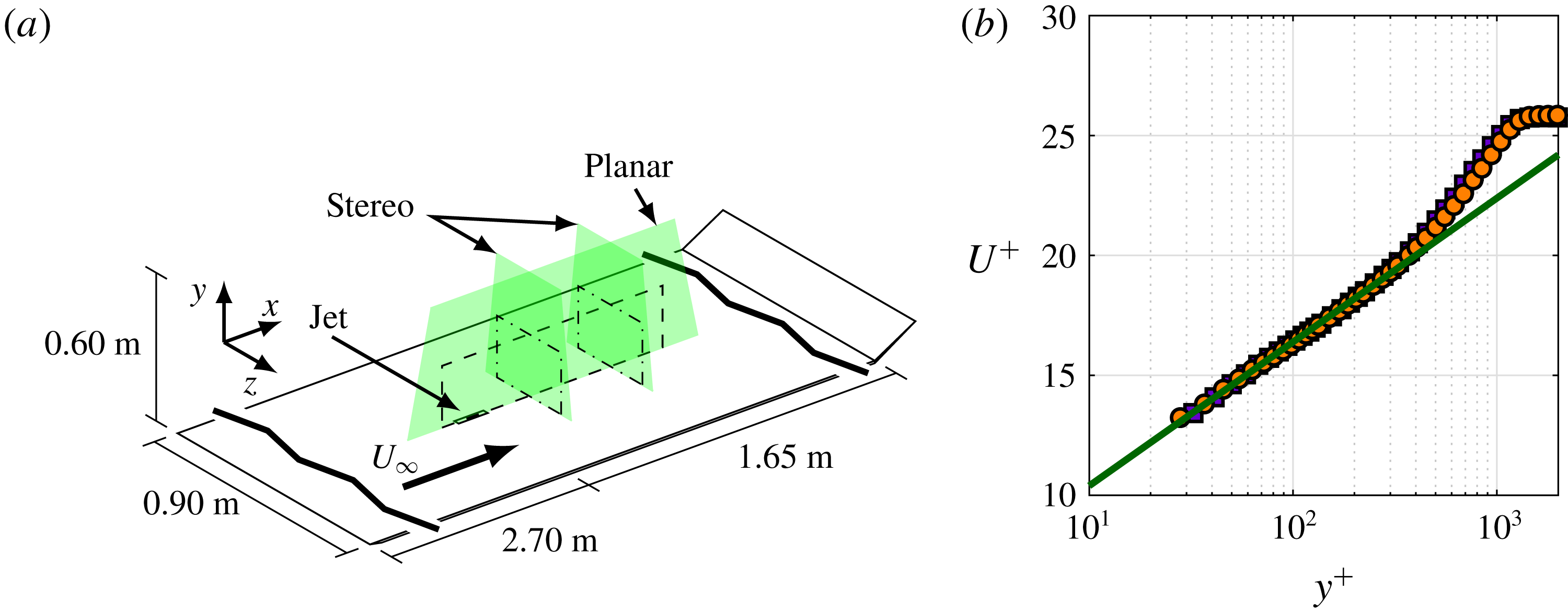
(a) Schematic of experimental set-up (not to scale). (b) Boundary-layer profiles of unperturbed flow at
 $x/\unicode[STIX]{x1D6FF}=-1$
(purple squares) and at
 $x/\unicode[STIX]{x1D6FF}=6$
(orange circles) compared to a log law with coefficients
 $\unicode[STIX]{x1D705}=0.384$
and
 $A=4.4$
(green line).

First, the measured momentum-flux deficit is presented in § 3.1. The three different sources of momentum deficit as introduced above are identified and discussed using these measurements. The measured vortical structures are reconstructed in § 3.2.1 and their induced velocity is calculated in § 3.2.2. This induced velocity is compared to the measured velocity deficit and the similarities/differences in the momentum-flux deficit for both cases are discussed. Using the measured vortical structures as an input, an inviscid-flow model is discussed in § 3.3 which predicts the evolution of a train of these structures. This model gives insight in the three-dimensional three-component velocity field as well as the deformation and evolution of the vortical structures.
2 Experimental set-up and procedures
2.1 Description of the flow and facility
Experiments are performed in the University of Southampton’s 3 ft by 2 ft suction wind tunnel. The tunnel is fitted with a false floor, creating a test section of
 $4.35$
m
 $\times$
0.60 m
 $\times$
0.90 m (
 $x\times y\times z$
, as defined in figure 1). Figure 1(a) presents a schematic of the experimental set-up. The boundary layer on the flat plate is tripped using a zip-zag tape fixed 3 cm downstream of the leading edge of the plate. The angle of the trailing-edge flap is adjusted to control the location of the stagnation point at the leading edge of the plate, ensuring a well defined and stable turbulent boundary layer. At a free-stream velocity of
 $U_{\infty }=10~\text{m}~\text{s}^{-1}$
, the turbulent boundary layer at the measurement station has a boundary-layer thickness (based on
 $U(\unicode[STIX]{x1D6FF})=0.99U_{\infty }$
) of
 $\unicode[STIX]{x1D6FF}=45$
mm. Boundary-layer profiles of the unperturbed flow (i.e. in the absence of the jet) are presented in figure 1(b) measured at
 $x/\unicode[STIX]{x1D6FF}=-1$
and
 $x/\unicode[STIX]{x1D6FF}=6$
. The overlap of these two measurements shows that the growth of the boundary layer over our measurement domain is negligible. The data are fitted to a log law with coefficients
 $\unicode[STIX]{x1D705}=0.384$
and
 $A=4.4$
(Marusic et al.
Reference Marusic, Monty, Hultmark and Smits2013). This fit indicates a friction velocity of
 $U_{\unicode[STIX]{x1D70F}}=0.38~\text{m}~\text{s}^{-1}$
(
 $Re_{\unicode[STIX]{x1D70F}}=1200$
).
2.2 Description of the synthetic jet actuator
A synthetic jet with a rectangular orifice exit of dimensions
 $l=13$
mm in the
 $x$
-direction and
 $d=1$
mm in the
 $z$
-direction is used. The exit of the jet is flush with the boundary-layer plate and the jet issues perpendicular into the boundary layer (i.e. in the
 $y$
-direction). The jet is driven by a loudspeaker, attached to a cavity of volume
 $1.85\times 10^{-5}$
m
 $^{3}$
and a nozzle with a neck length of 19.5 mm leading to the orifice exit. More details of the actuator can be found in Berk, Gomit & Ganapathisubramani (Reference Berk, Gomit and Ganapathisubramani2016). The jet velocity (
 $\bar{u}_{j}$
in (1.2)) is measured in the absence of the cross-flow. Six cases are considered for which the actuation parameters are given in table 1. These cases can be divided into a set of four Strouhal numbers for a fixed velocity ratio and a set of three velocity ratios for a fixed Strouhal number. For all cases the jet is operated using a sinusoidal waveform, leading to a near-sinusoidal velocity cycle.
Actuation parameters used for the different cases in the present study.

2.3 Measurement procedures
Velocity fields are measured using particle image velocimetry (PIV). Planar-PIV measurements (giving two-dimensional, two-component velocity fields) are taken in the
 $(x,y)$
-plane on the centreline of the orifice, spanning from
 $x=-2\unicode[STIX]{x1D6FF}$
to
 $7\unicode[STIX]{x1D6FF}$
and
 $y=0.05\unicode[STIX]{x1D6FF}$
to
 $2\unicode[STIX]{x1D6FF}$
. For two of the measured cases (
 $St=0.9$
,
 $r=0.88$
and
 $St=0.7$
,
 $r=1.35$
) a measurement error caused the measurement plane to end at
 $x=3\unicode[STIX]{x1D6FF}$
. For this measurement an array of three LaVision ImagerPro LX 16MP cameras is used. The planar velocity fields have a resolution of 0.34 mm per vector. Stereo-PIV measurements (giving two-dimensional, three-component velocity fields) are taken in the
 $(y,z)$
-plane at streamwise positions of
 $3\unicode[STIX]{x1D6FF}$
and
 $6\unicode[STIX]{x1D6FF}$
downstream of the orifice, with the plane spanning from
 $z=-1\unicode[STIX]{x1D6FF}$
to
 $1\unicode[STIX]{x1D6FF}$
and
 $y=0.05\unicode[STIX]{x1D6FF}$
to
 $2\unicode[STIX]{x1D6FF}$
. For this measurement two LaVision ImagerPro LX 16MP cameras are placed at opposite sides of the test section, pointing upstream with an included angle of 60 degrees. The stereo velocity fields have a resolution of 0.35 mm per vector. Measurements are taken phase locked to the actuation signal at eight equidistant phases of the jet. Each phase is averaged over 300 measurements. This reduces the uncertainty in the phase-averaged velocity in the region of interest to below 3 % (based on a 95 % confidence interval).
2.4 Use of velocity, vorticity and momentum
The background flow is removed in order to measure the strength of the vortical structures imposed on the background flow. In the present study the time-averaged incoming velocity components are used as proxy for the background flow, i.e.
 $$\begin{eqnarray}\displaystyle & \displaystyle u^{\ast }(x,y)=u(x,y)-u_{in}(y), & \displaystyle\end{eqnarray}$$
 $$\begin{eqnarray}\displaystyle & \displaystyle v^{\ast }(x,y)=v(x,y)-v_{in}(y)\approx v(x,y), & \displaystyle\end{eqnarray}$$
 $$\begin{eqnarray}\displaystyle & \displaystyle w^{\ast }(x,y)=w(x,y)-w_{in}(y)\approx w(x,y), & \displaystyle\end{eqnarray}$$
where
 $u$
,
 $v$
and
 $w$
indicate the streamwise, wall-normal and spanwise velocity components respectively,
 $u_{in}$
indicates the (time-averaged) incoming velocity and
 $u^{\ast }$
the velocity relative to the incoming flow. The incoming velocity profile is measured upstream of the actuator, averaged over
 $-1.5<x/\unicode[STIX]{x1D6FF}<-1.0$
. The spanwise and wall-normal components in the incoming boundary layer are found to be negligible. Using these relative components of velocity, the vorticity fields are given by
 $$\begin{eqnarray}\unicode[STIX]{x1D714}_{z}^{\ast }=\frac{\unicode[STIX]{x2202}v^{\ast }}{\unicode[STIX]{x2202}x}-\frac{\unicode[STIX]{x2202}u^{\ast }}{\unicode[STIX]{x2202}y},\end{eqnarray}$$
for the relative spanwise vorticity in the
 $(x,y)$
-plane and
 $$\begin{eqnarray}\unicode[STIX]{x1D714}_{x}^{\ast }=\frac{\unicode[STIX]{x2202}w^{\ast }}{\unicode[STIX]{x2202}y}-\frac{\unicode[STIX]{x2202}v^{\ast }}{\unicode[STIX]{x2202}z},\end{eqnarray}$$
for the relative streamwise vorticity in the
 $(z,y)$
-plane.
Vortices are identified in these vorticity fields using swirling strength (see Adrian, Christensen & Liu (Reference Adrian, Christensen and Liu2000)) which differentiates between vortices and shear layers. Unless noted otherwise, vorticity fields presented throughout this paper only show vorticity at locations identified by the swirling strength as belonging to a vortex.
In the present paper the terms momentum, momentum flux and streamwise momentum flux are used interchangeably to indicate the flow of streamwise momentum through a point or plane, i.e.
 ${\dot{P}}=\text{d}P/\text{d}t=\unicode[STIX]{x1D70C}u^{2}$
, where
 $\unicode[STIX]{x1D70C}$
is the density of the fluid. The momentum-flux deficit considered in this paper is based on the time-averaged velocities. The streamwise-momentum-flux deficit compared to the incoming flow is given by
 $$\begin{eqnarray}\unicode[STIX]{x0394}{\dot{P}}(x,y)=-(\unicode[STIX]{x1D70C}u^{2}(x,y)-\unicode[STIX]{x1D70C}u_{in}^{2}(y)).\end{eqnarray}$$
Using the relative velocity component defined in (2.1) this equals
 $$\begin{eqnarray}\unicode[STIX]{x0394}{\dot{P}}(x,y)=-\unicode[STIX]{x1D70C}((u^{\ast }+u_{in})^{2}-u_{in}^{2})=-\unicode[STIX]{x1D70C}((u^{\ast })^{2}+2u^{\ast }u_{in}),\end{eqnarray}$$
where
 $u^{\ast }$
is either the measured relative velocity or the reconstructed velocity induced by the vortical structures.
3 Results and discussion
As discussed above, the synthetic jet issuing into the turbulent boundary layer creates a momentum deficit in the cross-flow. The measured (streamwise) momentum deficit is presented and discussed in § 3.1. The different sources of momentum deficit are identified and discussed using this measured data. The momentum deficit induced by the vortical structures of the jet is reconstructed from the measured vorticity fields and discussed in § 3.2. An inviscid-flow model, predicting the evolution of a train of vortical structures, is presented in § 3.3. Throughout the paper maps of the velocity fields are presented for the
 $St=0.1$
,
 $r=0.88$
case. This lowest-
 $St$
case is chosen because it has the largest separation between subsequent structures. This makes the velocity fields clearer and clearly shows individual structures. Unless stated otherwise, presented analysis methods and conclusions are similar for all cases.
3.1 Measured momentum-flux deficit
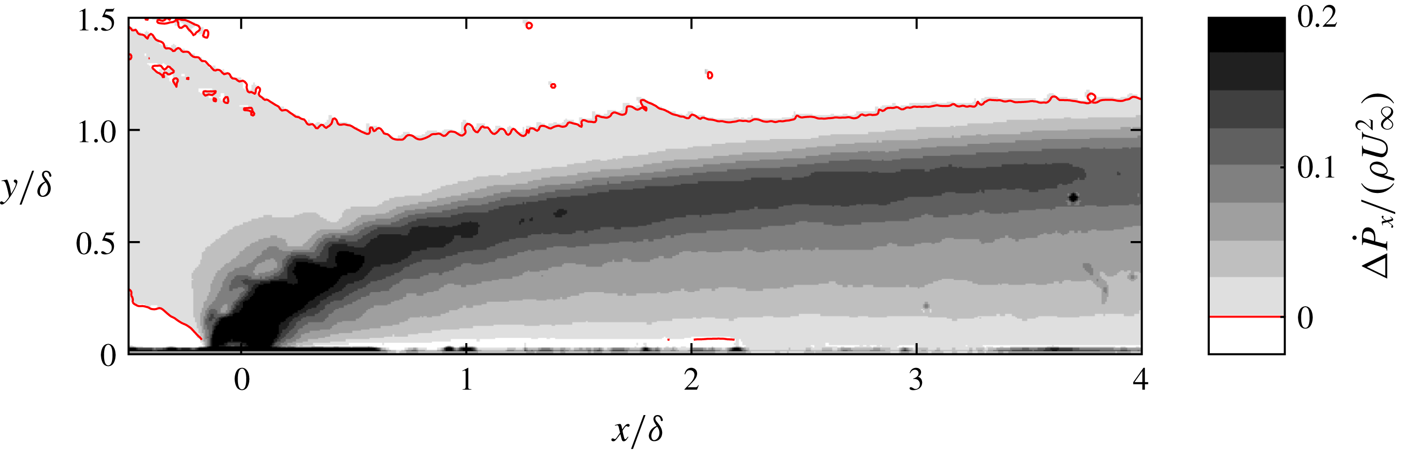
The momentum-flux deficit is calculated using (2.6). The momentum-flux deficit for the
 $St=0.1$
,
 $r=0.88$
case is presented in figure 2. A plume of streamwise-momentum-flux deficit originating from the orifice of the jet is visible, indicating that the jet creates a wake in the cross-flow. The red contour line in figure 2 indicates the wall-normal height above which the momentum-flux deficit is negative, meaning that the momentum flux has increased. It is assumed that the main mechanism behind this increase in momentum flux around the wake of the jet is the conservation of mass. This implies that the volume flow through each cross plane in the wind tunnel must be equal and therefore if the velocity is decreased in one area, the flow has to speed up around it. In addition, the flow might be accelerated above the wake by the induced velocity of vortical structures.
Measured momentum-flux deficit field for the
 $St=0.1$
,
 $r=0.88$
case. The red contour line indicates
 $\unicode[STIX]{x0394}{\dot{P}}=0$
.

The streamwise-momentum-flux deficit is evaluated as function of streamwise location by integrating in wall-normal direction as
 $$\begin{eqnarray}\unicode[STIX]{x0394}{\dot{P}}_{x}(x)=\frac{1}{\unicode[STIX]{x1D6FF}}\int \unicode[STIX]{x0394}{\dot{P}}(x,y)\,\text{d}y.\end{eqnarray}$$
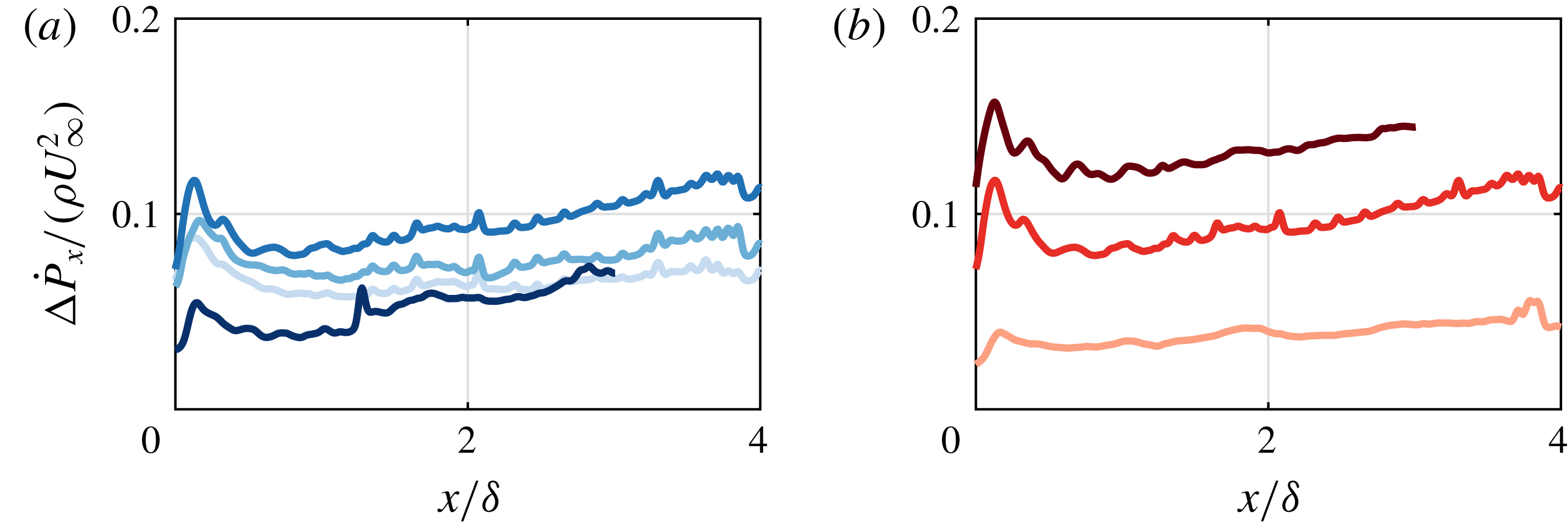
This integral is evaluated over the wall-normal extent of the wake (from the wall up to the contour line in figure 2). The momentum-flux deficit as a function of streamwise distance is presented for all six cases in figure 3.
Variation of measured momentum-flux deficit with (a) Strouhal number for
 $r=0.88$
and
 $St=0.1$
,
 $0.3$
,
 $0.7$
and
 $0.9$
(darker shades of blue for increasing
 $St$
) and with (b) velocity ratio for
 $St=0.7$
and
 $r=0.45$
,
 $0.88$
and
 $1.35$
(darker shades of red for increasing
 $r$
).

The variation of momentum-flux deficit with Strouhal number (see figure 3
a) shows that (for
 $0.1<St<0.7$
) the deficit slightly increases for increasing Strouhal number. For the highest Strouhal number (
 $St=0.9$
) the momentum-flux deficit is considerably lower. It is expected that this is caused by the actuation parameters of the synthetic jet approaching a formation criterion similar to the one proposed for synthetic jets in the absence of cross-flow by Holman et al. (Reference Holman, Utturkar, Mittal, Smith and Cattafesta2005). This criterion states that if the ratio of
 $\bar{u}_{j}/f$
is too low, vortices created by the jet will be re-ingested during the suction phase, thereby greatly reducing the effectiveness of the jet and ultimately leading to no jet being formed at all.
The variation of momentum-flux deficit with velocity ratio (see figure 3 b) shows that the momentum-flux deficit increases for an increasing velocity ratio. This variation is intuitive as the velocity ratio is directly related to the strength (either fluidic power, total circulation or total ejected volume) of the jet.
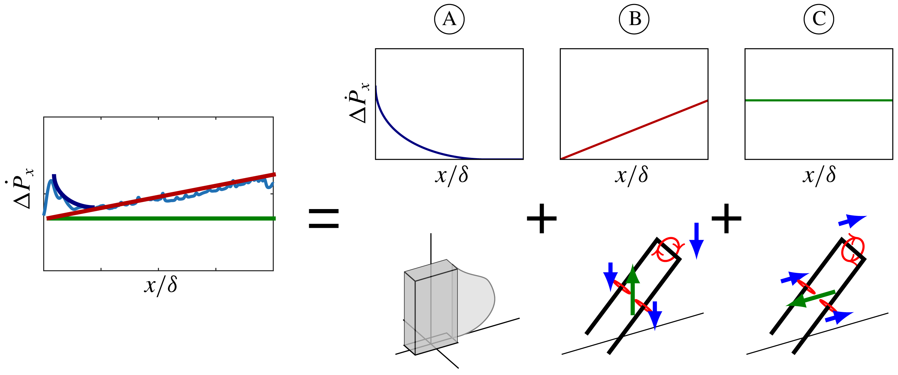
Schematic representation of momentum deficit as a sum of (A) viscous blockage, (B) increased skin friction due to down-wash and (C) induced streamwise velocity.

The momentum-flux deficit for each case shows the same trend; a sharp increase followed by a decrease, forming a peak shortly downstream of the jet, after which it shows an almost linear increase. It can be hypothesized that this trend is due to the different sources of momentum deficit. These sources are represented schematically in figure 4. Three sources of momentum deficit are identified; viscous blockage (A in figure 4), increased skin friction (B) and induced velocity (C). Note that other (unforeseen) sources of momentum deficit might be present and could be causing the described trends. The peak immediately downstream of the orifice could be reconciled as the effect of viscous blockage of the cross-flow by the jet. This is somewhat analogous to blockage by a slender column, which will create a quickly recovering blockage wake as presented schematically in figure 4(A) (e.g. Sumner, Heseltine & Dansereau (Reference Sumner, Heseltine and Dansereau2004)). The main difference is that instead of transferring the momentum to the wall as a solid object does, the jet fluid retains this momentum and uses it to accelerate as discussed in § 1.
The vortical structures created by the synthetic jet (the shape of these structures will be discussed in § 3.2) induce a flow in the wall-normal direction as shown schematically in figure 4(B). This flow is away from the wall between the legs of the structure and towards the wall outside the legs. In the literature this effect is often referred to as up-wash of low-momentum fluid (e.g. Rathnasingham & Breuer Reference Rathnasingham and Breuer2003), which is only one half of the story since up-wash and down-wash balance each other. This effect does however redistribute regions of low and high momentum, effectively increasing the velocity close to the surface and therewith the skin friction. This increase in skin friction will act as a momentum sink, leading to a constant rate of increase of the momentum-flux deficit as shown in figure 4(B). In the present study we do not measure this increase in skin friction directly and the measured constant rate of increase of the momentum-flux deficit might be caused by an unforeseen source of momentum loss.
The same vortical structures also induce a velocity component in the streamwise direction as shown schematically in figure 4(C). Between the legs of the structure, at the centreline of the jet this component is mainly in the direction opposite to the cross-flow, thereby directly inducing a velocity deficit and increasing the momentum-flux deficit. For a constant geometry and strength of the vortical structure, the induced streamwise-momentum-flux deficit is constant as represented schematically in figure 4(C).
A far-field region can be defined from both the trajectory and the momentum-flux deficit as
 $x/\unicode[STIX]{x1D6FF}>1$
. In this far-field region, the effect of the vertical velocity on the trajectory (see figure 2) and the effect of viscous blockage (see figure 3) have diminished. Unless stated otherwise, in the remainder of this paper, only the far field is considered.
The induced momentum-flux deficit in the far field, as presented schematically in figure 4(C) is reconstructed from the data and quantified in § 3.2. An inviscid-flow model, predicting the evolution of a train of vortical structures is presented in § 3.3. This model predicts the induced velocity based on the geometry and strength (circulation) of an input structure.
3.2 Induced momentum-flux deficit
The geometry and strength (i.e. circulation) of the vortical structures created by the synthetic jet are determined using a combination of planar- and stereo-PIV. The reconstruction of these vortical structures is discussed in § 3.2.1. Using these reconstructed structures, the vortex-induced velocity is calculated using the Biot–Savart law in § 3.2.2. The
 $St=0.1$
,
 $r=0.88$
case is used to exemplify the reconstruction method.
3.2.1 Reconstruction of vortical structures
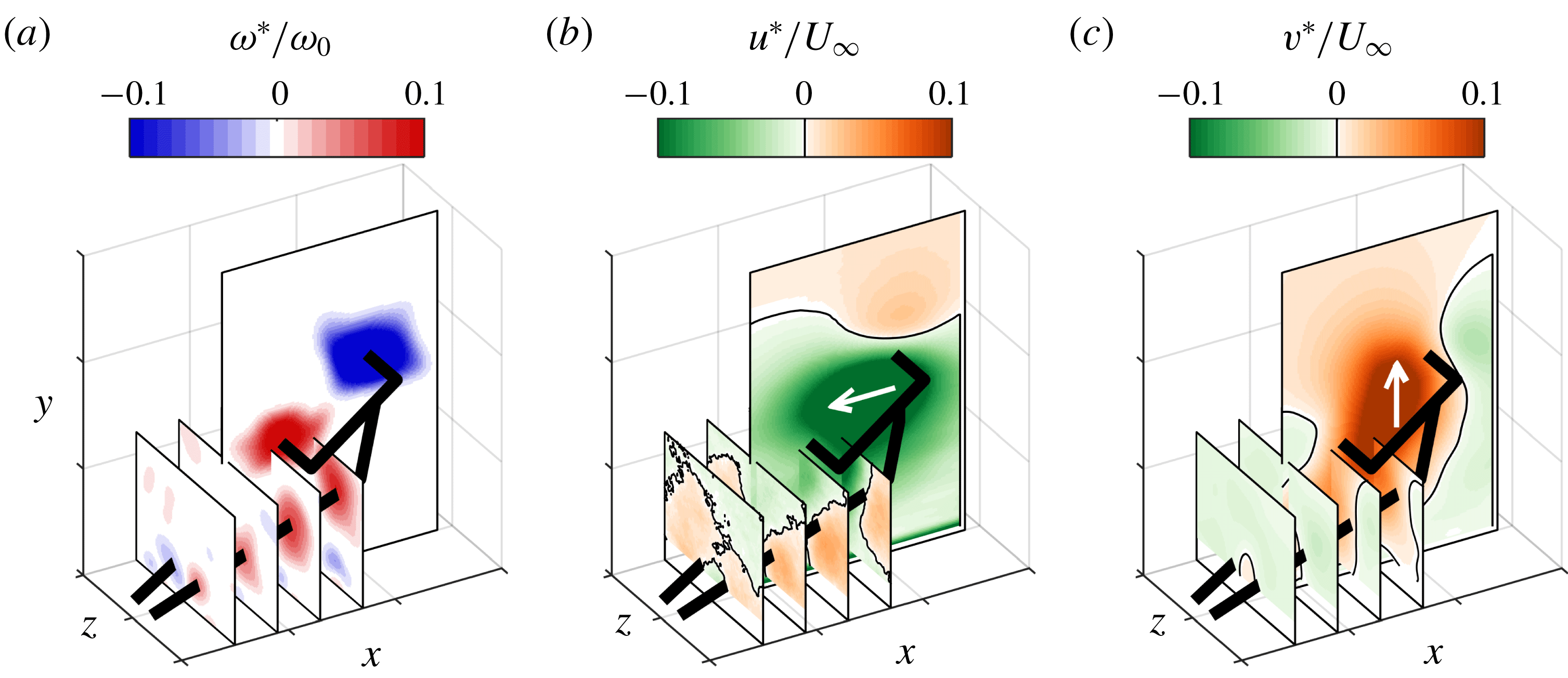
As discussed above, the interaction of a synthetic jet with a turbulent boundary layer is expected to result in the creation of hairpin-like vortical structures. The geometry of these structures is reconstructed from a combination of different measurement planes as presented in figure 5. The four presented spanwise–wall-normal planes are all measured at the same streamwise location during different phases of the jet. The transformation of this phase difference to a streamwise displacement is discussed below.
Three-dimensional reconstruction of a single vortical structure with (a) vorticity (
 $\unicode[STIX]{x1D714}_{z}^{\ast }$
in the
 $(x,y)$
-plane and
 $\unicode[STIX]{x1D714}_{x}^{\ast }$
in the
 $(y,z)$
-plane). (b) Streamwise velocity and (c) wall-normal velocity.

The observed vorticity fields do not resemble a classical hairpin. Instead, the vortical structure seems to consist of a tilted vortex ring with legs originating from the sides of the ring as indicated by the thick black line in figure 5. The shape of this structure can be explained from the interaction of the synthetic jet with the boundary layer. During formation, the vortex ring created by the synthetic jet entrains vorticity from the cross-flow boundary layer. This entrained vorticity has the opposite sign to the vorticity in the upstream side of the vortex ring but equal sign to the downstream side, leading to a redistribution of vorticity in the vortex ring. According to Helmholtz’s vortex theorems (for inviscid flow) the strength of a vortex filament is constant along its length and cannot end in a fluid. This means that (for inviscid flow) vorticity can only vary along a ring in the presence of a side branch. These branches are formed at the spanwise sides of the ring, leading from the ring to the surface and forming the observed legs. The strength of the legs is then given by the difference in strength between the two sides of the vortex ring. The asymmetry in vorticity distribution along the ring also causes tilting of the ring as the downstream side of the ring (with higher circulation) has a stronger self-induced vertical velocity. This tilting has previously been observed and explained for vortex rings in a shear flow by Lim et al. (Reference Lim, Lua and Thet2008) and Cheng et al. (Reference Cheng, Lou and Lim2009).
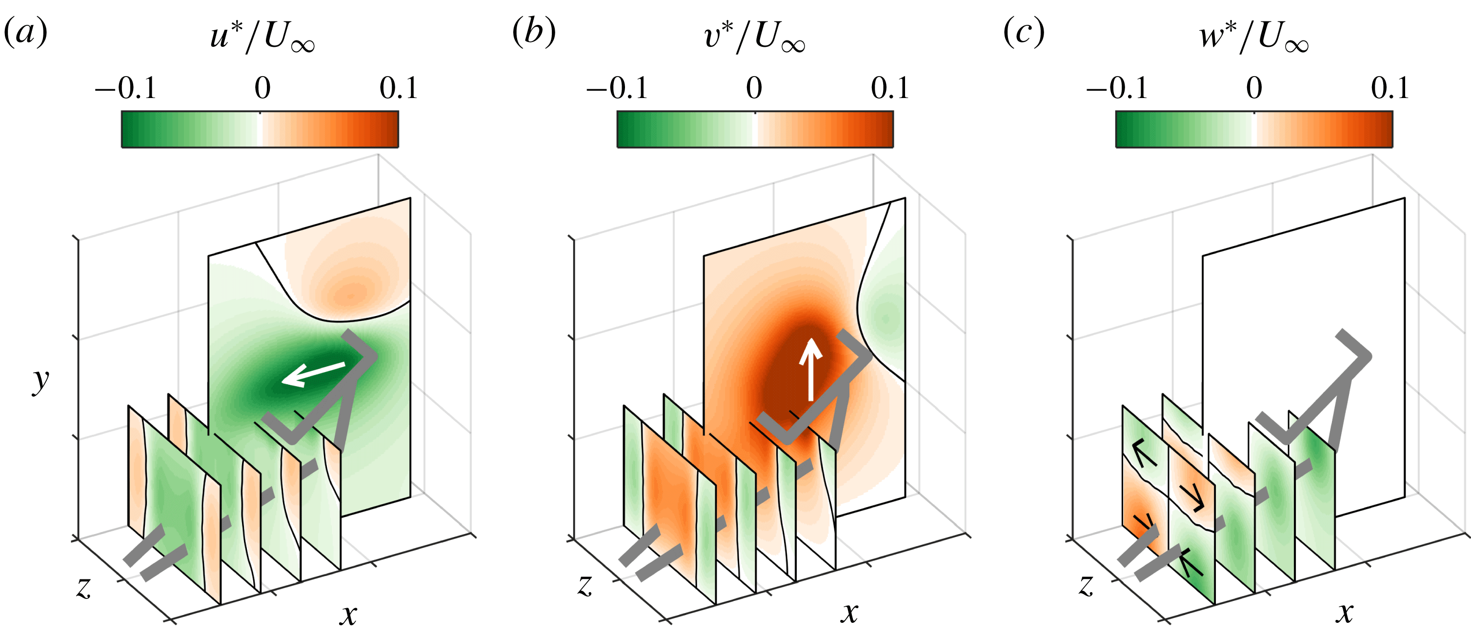
The streamwise and wall-normal velocity components measured around the vortical structure are presented in figure 5(b,c). Although the shape of the structure is more complicated than that of a single hairpin, the velocity components are similar to those expected from a hairpin (see the schematic representations in figure 4B,C). The streamwise velocity field is dominated by negative velocity (opposite to the cross-flow direction) within the vortex ring and between the legs. The wall-normal velocity field is dominated by a positive velocity (away from the wall) within the ring and between the legs. The velocity components outside the structure are in the opposite direction, due to the circular motion around vortical filaments. Inside the vortical structure the streamwise and wall-normal velocity components induced by the different parts of the structure act in the same direction, leading to a high velocity. Outside the structure the components induced by the different parts of the structure act in opposite directions, leading to a relatively low induced velocity.
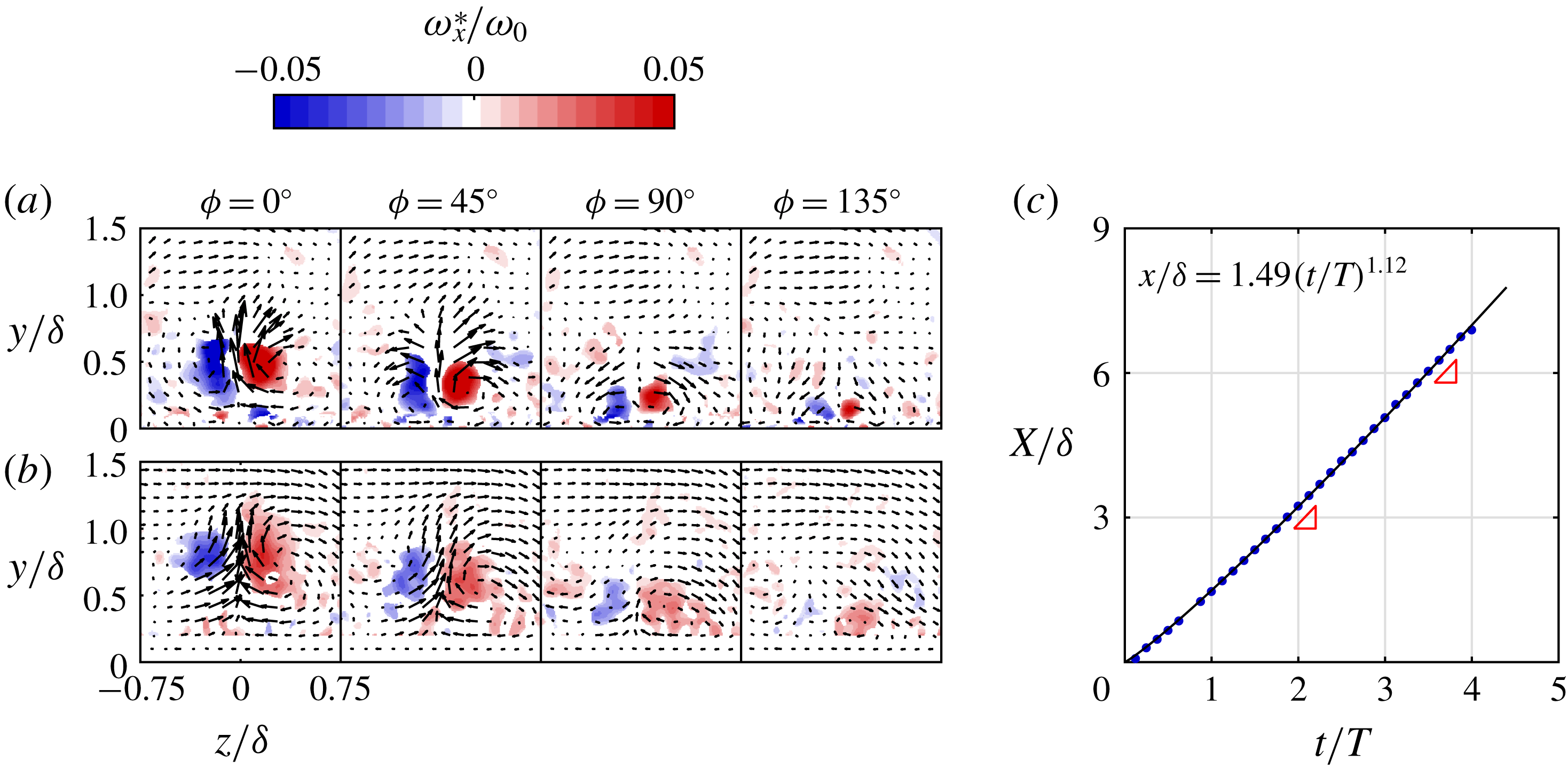
The streamwise vorticity fields of the legs are presented in more detail and for both the
 $x/\unicode[STIX]{x1D6FF}=3$
and
 $6$
locations in figure 6. The legs can be identified as counter-rotating vortex pairs. The exact position of the legs is defined as the weighted centre of vorticity, calculated for both vortices independently and averaged over the presented range (i.e.
 $-0.75<z/\unicode[STIX]{x1D6FF}<0.75$
and
 $0<y/\unicode[STIX]{x1D6FF}<1.5$
). As time (i.e. phase) increases, the vortex pair moves closer to the surface, corresponding to the inclination of the legs as in figure 5. For both downstream locations the vortex pair is only visible during the four presented phases (out of a total of eight phases).
Streamwise vorticity measured using stereo-PIV during four phases, showing the legs of the vortical structure at
 $x/\unicode[STIX]{x1D6FF}=3$
(a) and
 $x/\unicode[STIX]{x1D6FF}=6$
(b). Streamwise position as function of time (c) tracked using planar-PIV. The advection velocity of the structures, given by the slope indicated by the red triangles defines the streamwise separation distance between subsequent fields in (a) and (b).

Although the structure evolves between
 $x/\unicode[STIX]{x1D6FF}=3$
and
 $6$
, the deformation is small compared to the downstream displacement. Therefore, the structure is assumed to be ‘frozen’ in order to translate the temporal spacing to a spatial distance using the advection velocity (similar to Taylor’s hypothesis). This velocity is determined by tracking the head of the vortical structure through time in the streamwise–wall-normal plane. The tracked streamwise position is presented in figure 6(c). The streamwise evolution shows a rapid acceleration to a relatively constant advection velocity. This evolution is fitted to a power law (indicated by the black line) which gives an accurate representation. The streamwise advection velocity is calculated as the derivative of this power law. The advection velocities at
 $x/\unicode[STIX]{x1D6FF}=3$
and 6 (
 $0.88U_{\infty }$
and
 $0.95U_{\infty }$
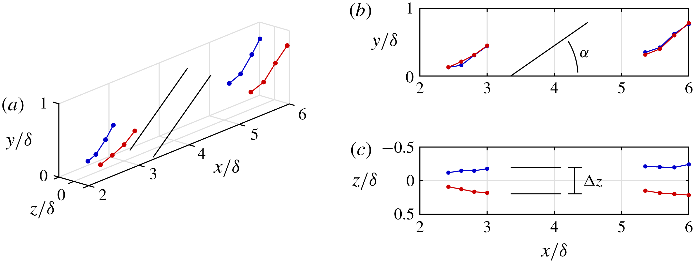
respectively) are used to translate the phase differences in figure 6(a,b) to a streamwise separation between subsequent vorticity fields. The combination of this streamwise location of the measurement planes with the spanwise and wall-normal location of the vortices as determined from these planes leads to the three-dimensional geometry of the legs as presented in figure 7.
Measured geometry of the legs of the vortical structure at
 $x/\unicode[STIX]{x1D6FF}=3$
and
 $6$
. Colours indicate sign of streamwise vorticity (red positive). The black structure indicates the modelled geometry with
 $\unicode[STIX]{x0394}z=20d$
and
 $\unicode[STIX]{x1D6FC}=35^{\circ }$
.

The legs of the hairpin are presented at streamwise positions
 $x/\unicode[STIX]{x1D6FF}=3$
and
 $x/\unicode[STIX]{x1D6FF}=6$
. The side view presented in figure 7(b) shows that, although the structure moves away from the wall, the inclination angle of the legs compared to the wall is relatively constant. The top view presented in figure 7(c) shows that the legs are parallel to each other and have a relatively constant separation distance. The black lines show a modelled pair of legs with an inclination angle of
 $\unicode[STIX]{x1D6FC}=35^{\circ }$
and a spanwise separation of
 $\unicode[STIX]{x0394}z=20d$
(for
 $d=1$
mm the orifice width) which closely matches the data. The inclination angle and spanwise separation for other cases are found to be similar.
3.2.2 Calculation of vortex-induced velocity
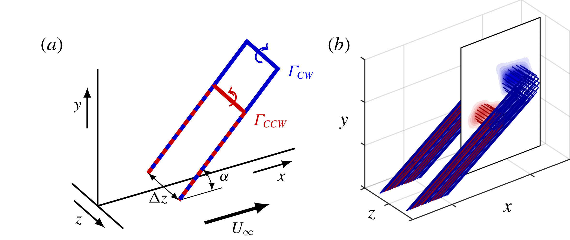
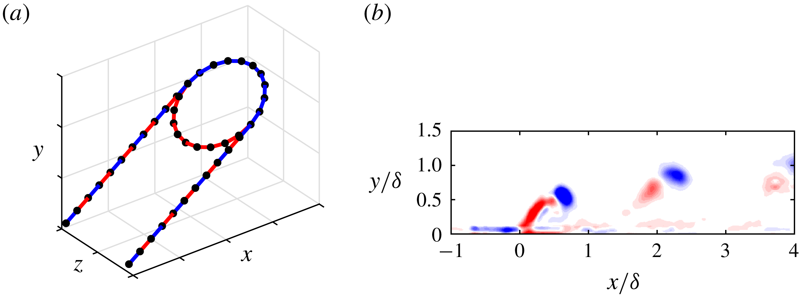
The geometry of the vortical structure is simplified by modelling it as the combination of two hairpins as presented in figure 8(a). These two hairpins originate from the counterrotating vortices measured in the head of the structure. The vortical filaments forming these hairpins have constant circulation along their length given by
 $\unicode[STIX]{x1D6E4}_{CW}$
and
 $\unicode[STIX]{x1D6E4}_{CCW}$
, equal to the measured circulation of the clockwise and counter-clockwise vortices respectively. In line with the above discussion
 $|\unicode[STIX]{x1D6E4}_{CW}|>|\unicode[STIX]{x1D6E4}_{CCW}|$
. Both hairpins overlap in the legs of the structure, leading to partial cancellation of their effect. The velocity induced by the combination of these legs is equal to a velocity induced by legs of magnitude
 $\unicode[STIX]{x1D6E4}_{leg}=\unicode[STIX]{x1D6E4}_{CW}+\unicode[STIX]{x1D6E4}_{CCW}$
. The geometry of the legs is fully determined by the vorticity fields in the
 $(z,y)$
-plane as discussed above. Using the constant spanwise separation
 $\unicode[STIX]{x0394}z$
and inclination angle
 $\unicode[STIX]{x1D6FC}$
to describe these legs, only the position and circulation of the head, measured from the vorticity field in the
 $(x,y)$
-plane is required to fully reconstruct the hairpin vortices.
Simplified geometry of the vortical structure modelled as two counter-rotating hairpins (a) and implementation by using each data point as a separate hairpin (b).

Instead of using a single hairpin per vortex, a hairpin is modelled at each data point as presented in figure 8(b). Using each data point of the vorticity fields enables a more representative description of the vorticity distribution. The circulation of each filament is then given by
 $\unicode[STIX]{x1D6E4}=\unicode[STIX]{x1D714}_{z}^{\ast }\unicode[STIX]{x0394}x\unicode[STIX]{x0394}y$
, which is the area integral of vorticity
 $\unicode[STIX]{x1D714}_{z}^{\ast }$
for data with grid spacing
 $\unicode[STIX]{x0394}x$
and
 $\unicode[STIX]{x0394}y$
. For numerical purposes, each filament is described using a finite number of three-dimensional line segments, whose geometry is described by
 $\boldsymbol{d}\boldsymbol{s}$
. The Biot–Savart law states that the velocity induced by a segment (
 $\boldsymbol{u}_{ind,s}$
) on any point
 $(x,y,z)$
at distance
 $\boldsymbol{\ell }$
from the segment is given by
 $$\begin{eqnarray}\boldsymbol{u}_{ind,s}(x,y,z)=\frac{\unicode[STIX]{x1D6E4}}{4\unicode[STIX]{x03C0}}\frac{\boldsymbol{d}\boldsymbol{s}\times \boldsymbol{\ell }}{|\boldsymbol{\ell }|^{3}}.\end{eqnarray}$$
The full velocity
 $\boldsymbol{u}_{ind}$
induced at a given point is calculated by summing over the velocities induced by all segments in all filaments,
 $\boldsymbol{u}_{ind}(x,y,z)=\sum \boldsymbol{u}_{ind,s}(x,y,z)$
.
The three velocity components induced by the filaments in figure 8(b) are presented in figure 9. These velocity fields are the induced velocity components reconstructed from the measured velocity fields in figure 5. The measured and induced streamwise and wall-normal components (
 $u^{\ast }$
and
 $v^{\ast }$
) are qualitatively similar. In general, the velocity within the structure (i.e. between the legs and inside the ring) is in the streamwise direction opposite to the cross-flow and the wall-normal direction away from the wall, while the velocity outside the structure is in the opposite direction. The spanwise component of the induced velocity is presented in figure 9(c). Due to symmetry enforced by the hairpin model the spanwise component in the symmetry plane (
 $z=0$
) is zero.
Velocity induced by the three-dimensional vortical structure.

The velocity fields in the spanwise–wall-normal plane located at
 $x/\unicode[STIX]{x1D6FF}=3$
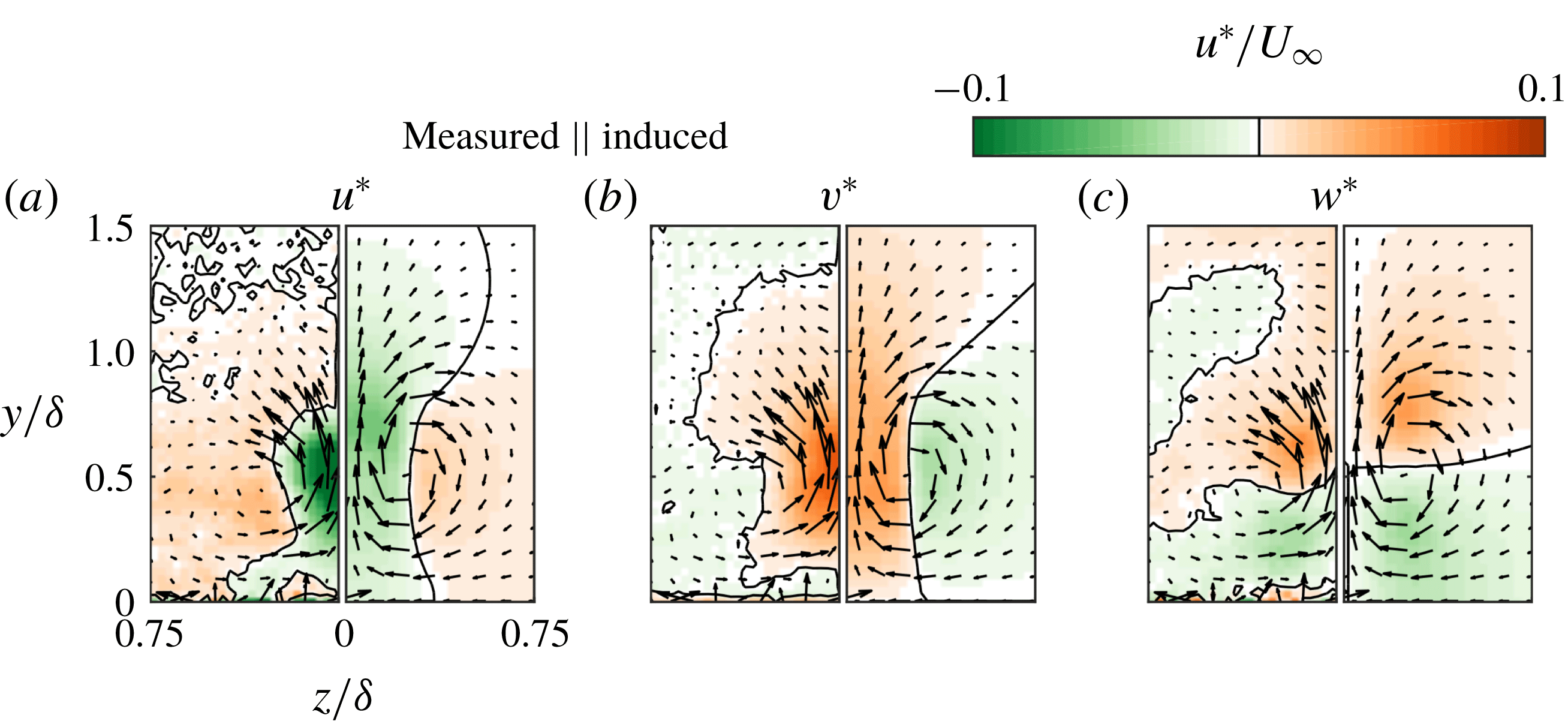
are presented in more detail for a single phase in figure 10. The presented phase shows a cross-section of the legs of the vortical structure. The streamwise, wall-normal and spanwise velocity components are presented in figures 10(a), 10(b) and 10(c), respectively. Each figure combines the measured velocity field (left, mirrored) with the induced velocity field (right) using the symmetry across
 $z/\unicode[STIX]{x1D6FF}=0$
. Qualitatively the induced velocity fields are largely similar to the measured velocity fields. The streamwise component (a) shows a velocity deficit between the legs and a velocity increase outside the legs. The measured velocity field indicates an increase in velocity above the legs while this is not present in the induced velocity field. This difference will be discussed below. The wall-normal component (b) indicates a velocity away from the wall between the legs and a velocity towards the wall outside the legs. These vertical motions redistribute regions of high and low momentum as will be discussed below. The spanwise component (c) indicates a velocity towards the centreline (
 $z/\unicode[STIX]{x1D6FF}=0$
) underneath the legs and a velocity away from the centreline above the legs. The combination of the spanwise and wall-normal components indicates a circular motion around each leg as can be expected for the flow around a vortical filament.
Comparison of phase-locked stereo-PIV data at
 $x/\unicode[STIX]{x1D6FF}=3$
(left half of plots, mirrored) to the computed induced velocity (right half) for the (a) streamwise, (b) wall-normal and (c) spanwise velocity components.

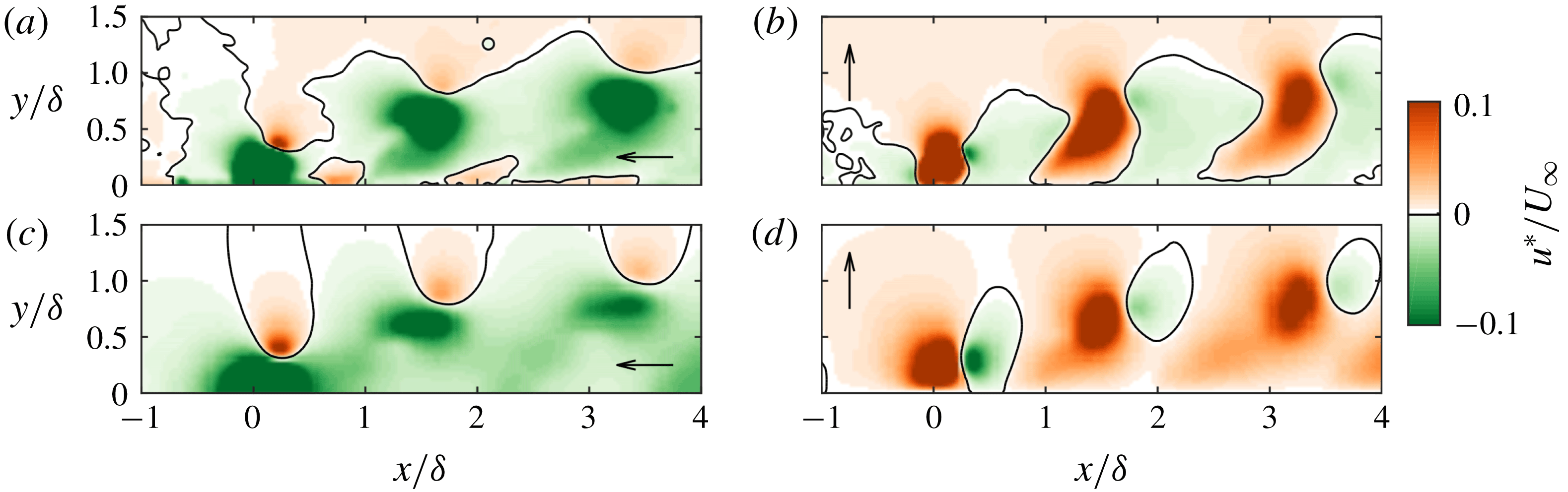
The velocity fields in the streamwise–wall-normal plane at
 $z/\unicode[STIX]{x1D6FF}=0$
are presented for a single phase in figure 11. The presented streamwise extent shows the velocity fields associated with a train of three subsequent vortical structures. Measured (a,b) and induced (c,d) velocity fields are compared for the streamwise (a,c) and wall-normal (b,d) components. Although the strength and wall-normal location of the three structures varies, the velocity fields surrounding these structures are qualitatively similar.
Comparison of phase-locked planar-PIV data at
 $z/\unicode[STIX]{x1D6FF}=0$
(a,b) to the computed induced velocity (c,d) for the streamwise (a,c) and wall-normal (b,d) components.

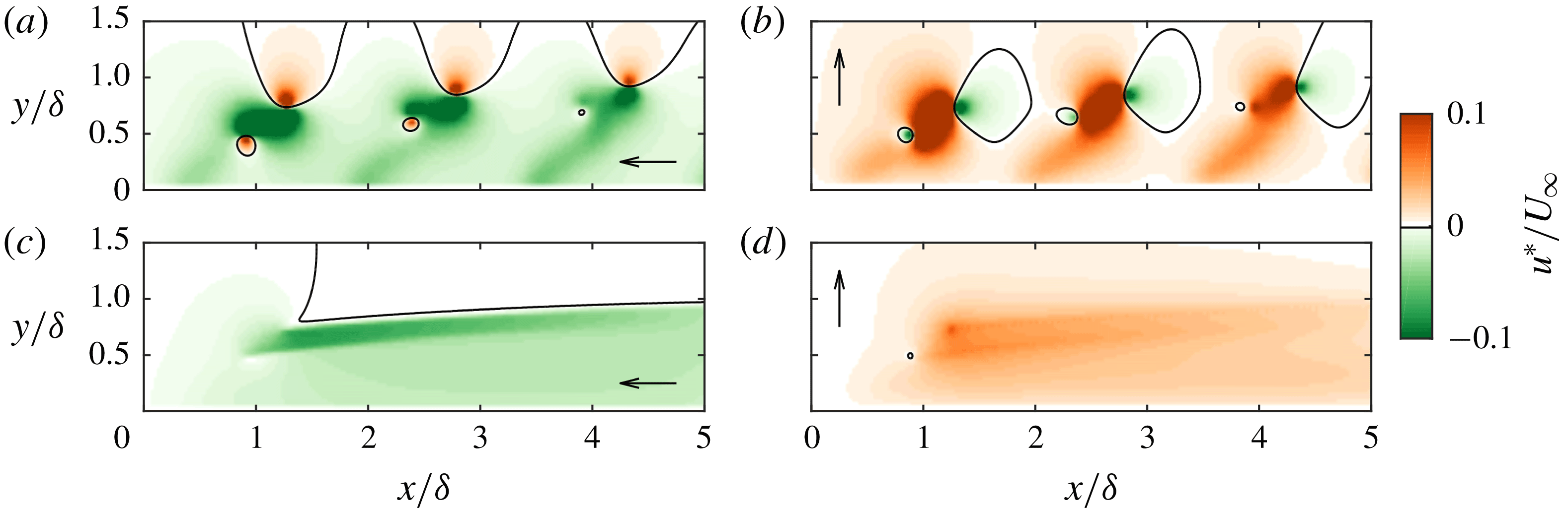
Time-averaged velocity fields in the streamwise–wall-normal plane at
 $z/\unicode[STIX]{x1D6FF}=0$
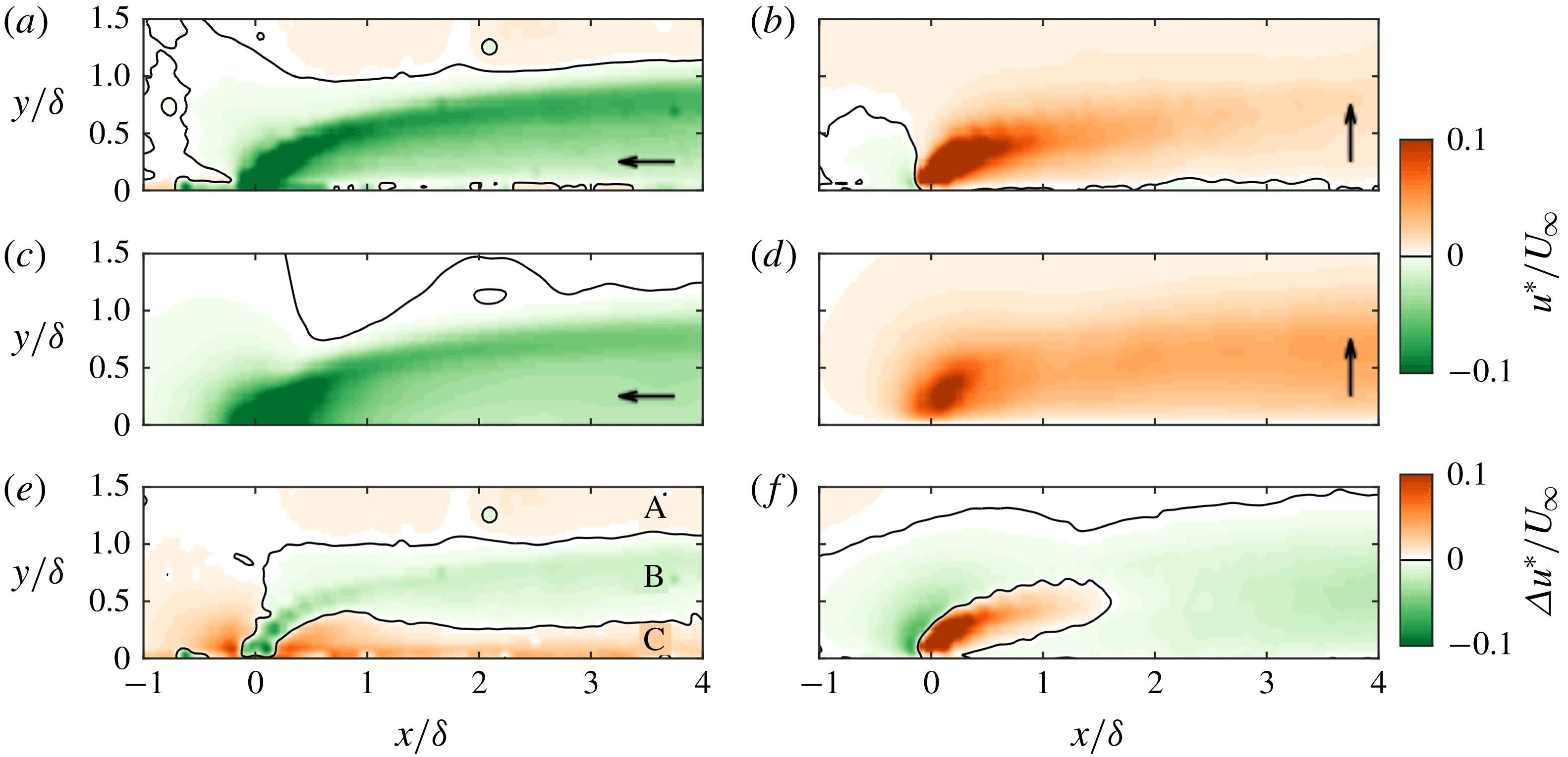
, averaged over eight phases, are presented in figure 12. Measured (a) and induced (c) streamwise velocity components are qualitatively similar. The difference between the two, defined as
 $\unicode[STIX]{x0394}u^{\ast }=u_{meas}^{\ast }-u_{ind}^{\ast }$
(e) shows three regions in the far field (i.e.
 $x/\unicode[STIX]{x1D6FF}>1$
) where the measured and induced components are different. Region A, above the wake of the jet (approximately at
 $y/\unicode[STIX]{x1D6FF}>1.0$
), shows a higher measured than induced velocity. It is expected that this is caused by the conservation of mass through cross-planes in the wind tunnel. As the incoming velocity is slowed down in part of this plane (due to the wake of the jet), the velocity of the surrounding flow has to increase to keep the same mass flux through each plane. The difference in region B, approximately at
 $0.3<y/\unicode[STIX]{x1D6FF}<1.0$
, indicates a measured velocity that is lower than the induced velocity (i.e. a stronger wake). It is assumed that this is due to the up-wash of low-momentum fluid as caused by the vertical component of the induced velocity. Similarly, region C (approximately at
 $y/\unicode[STIX]{x1D6FF}<0.3$
) indicates a higher measured than induced velocity. Analogously to the up-wash in region B it is assumed that this increase in velocity is caused by the down-wash of high-momentum fluid. The spanwise–wall-normal planes in figure 10 showed that the vertical component of the velocity field consists of upward motions between the legs and downward motions next to the legs, i.e. low-momentum fluid is removed from the wall between the legs of the structure while high-momentum fluid is transported towards the wall outside the legs.
Time-averaged measured and induced wall-normal components are presented in figure 12(b,d). The measured and induced velocity fields are qualitatively very similar and are both dominated by a velocity away from the wall. The difference between the two cases (
 $\unicode[STIX]{x0394}v^{\ast }=v_{meas}^{\ast }-v_{ind}^{\ast }$
) (f) indicates that the measured vertical velocity is much higher than the induced velocity in the core of the jet but lower just upstream of the jet. This is caused by the fact that the jet has a given wall-normal velocity (
 $\bar{u}_{j}$
) at the exit of the jet. This exit velocity is present in the measured velocity field, but not in the induced field, causing the core of the jet to be stronger for the measured case. Since synthetic jets are formed entirely from the surrounding fluid by alternating blowing and suction cycles, the flow upstream of the actuator is ingested into the jet as can be seen from the negative vertical velocity in the measured velocity field. In the far field (
 $x/\unicode[STIX]{x1D6FF}>1$
), the wall-normal velocity is over-predicted in most of the flow field. It is assumed that this is caused by the boundary layer compensating for the upward motion of vortical structures. With these structures moving upward due to their induced velocity a low pressure region is created underneath these structures. It can be assumed that the flow between subsequent structures is downward to compensate this pressure difference. This viscous effect leads to the over-prediction of wall-normal velocity as observed in figure 12.
Comparison of time-averaged planar-PIV data at
 $z/\unicode[STIX]{x1D6FF}=0$
(a,b) to the computed induced velocity (c,d) as well as the difference defined as
 $\unicode[STIX]{x0394}u^{\ast }=u_{meas}^{\ast }-u_{ind}^{\ast }$
(e,f) for the streamwise (a,c,e) and wall-normal (b,d,f) components.

The streamwise-momentum-flux deficit (
 $\unicode[STIX]{x0394}{\dot{P}}_{x}$
) as was presented for the measured cases in figure 3 is recalculated based on the induced velocity only. This induced streamwise-momentum-flux deficit is presented in figure 13. Note that for the
 $r=0.88$
,
 $St=0.9$
and
 $r=1.35$
,
 $St=0.7$
cases the measurement plane is only up to
 $x/\unicode[STIX]{x1D6FF}=3$
. Due to the reconstruction of hairpin structures based on the location of the heads (i.e. based on the most downstream part of the structures) the end of the measurement plane has an influence upstream. This is visible in figure 13 by the decline in induced momentum-flux deficit for these two cases shortly before reaching
 $x/\unicode[STIX]{x1D6FF}=3$
. Apart from this artificial decline, the induced deficit is relatively constant with streamwise location for all cases.
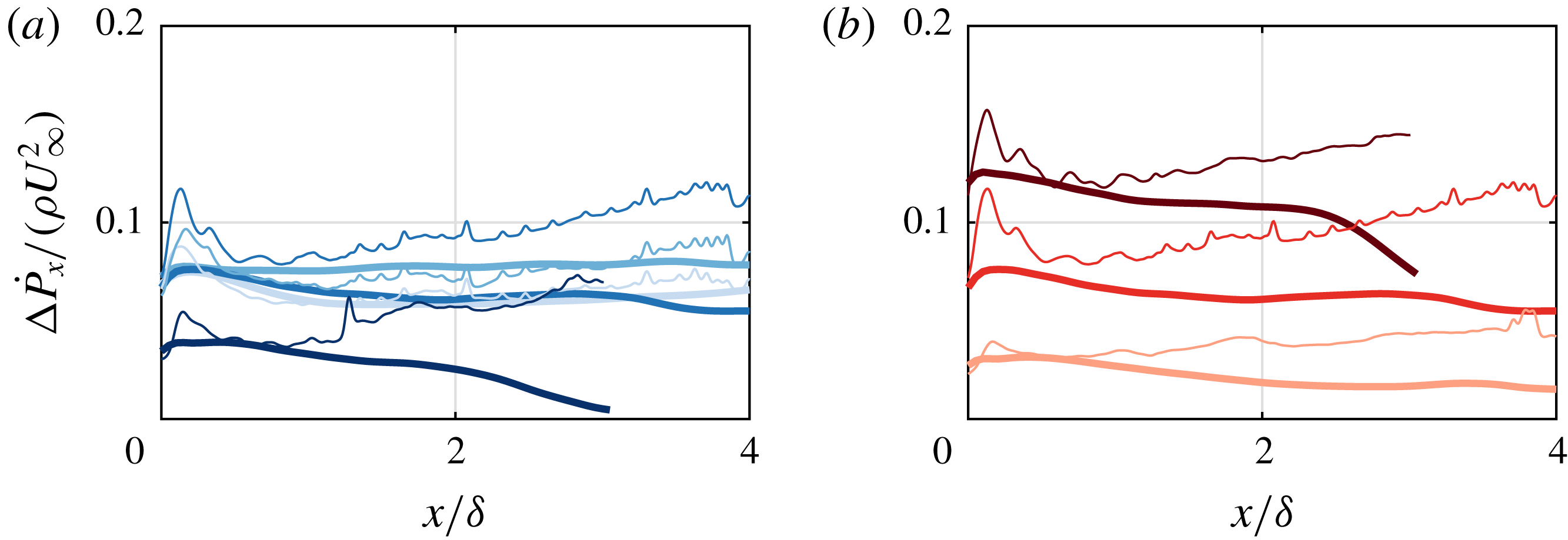
Figure 13(a) presents the induced momentum-flux deficit for different Strouhal numbers. For the three lowest Strouhal numbers the induced deficit is relatively equal. This can be explained using the theoretical circulation of vortex rings produced by the synthetic jet. During the formation of a vortex ring at the jet exit, the circulation grows with
 $\text{d}\unicode[STIX]{x1D6E4}/\text{d}t\approx u^{2}(t)/2$
(Shariff & Leonard Reference Shariff and Leonard1992), where
 $u(t)$
is the instantaneous centreline velocity. For a harmonic velocity cycle as used in the present study this implies that the circulation of a single structure (i.e. created during one cycle) scales with
 $\unicode[STIX]{x1D6E4}\propto \bar{u}_{j}^{2}/f$
. The number of these structures created per unit time equals the frequency causing the time-averaged circulation,
 $\unicode[STIX]{x1D6E4}_{TA}\propto \bar{u}_{j}^{2}$
, to be independent of frequency. This leads to an invariability of the strength of the train of vortices – and therewith the induced momentum flux with Strouhal number. As discussed above, for high Strouhal numbers the jet formation criterion is approached, leading to (partial) re-ingestion of circulation during the suction phase of the jet. This leads to a lower strength of the vortical structures for
 $St=0.9$
, explaining the lower induced momentum-flux deficit.
The induced streamwise-momentum-flux deficit is presented for different velocity ratios in figure 13(b). The induced deficit increases with velocity ratio. This can be expected from the dependence of the time-averaged circulation on the jet velocity.
Variation of induced momentum-flux deficit (thick lines) with (a) Strouhal number for
 $r=0.88$
and
 $St=0.1$
,
 $0.3$
,
 $0.7$
and
 $0.9$
(darker shades of blue for increasing
 $St$
) and with (b) velocity ratio for
 $St=0.7$
and
 $r=0.45$
,
 $0.88$
and
 $1.35$
(darker shades of red for increasing
 $r$
). Thin lines correspond to the measured momentum-flux deficit.

The induced momentum-flux deficit is compared to the measured momentum-flux deficit (thin lines in figure 13). For the two lowest Strouhal numbers (lightest blue lines) the measured momentum-flux deficit (downstream of the peak caused by viscous blockage) is similar to the induced momentum-flux deficit, indicating that the momentum deficit is almost entirely caused by the induced velocity. For the higher Strouhal numbers, as well as for the different velocity ratios, the measured momentum-flux deficit is larger than the induced momentum-flux deficit. This difference increases linearly with downstream distance, suggesting a constant momentum sink. As discussed alongside figure 4 it is assumed that this constant rate of increase in momentum-flux deficit with downstream distance is caused by a constant increase in skin friction. The absence of this difference for the lowest Strouhal numbers could be caused by the fact that in these cases the separation between subsequent vortical structures is large enough for the flow to recover between structures. For higher Strouhal numbers the separation between structures is smaller which does not give the flow near the surface time or space to recover, leading to an increase in velocity close to the wall (due to down-wash of high-momentum fluid) and subsequently an increase in skin friction.
3.3 Inviscid-flow model
An inviscid-flow model is developed which describes the temporal evolution of a train of vortical structures. The Matlab code for the model is provided in the supplementary material available at https://doi.org/10.1017/jfm.2019.279. The model is based on an input vortical structure which propagation velocity is a combination of a specified cross-flow advection velocity, its self-induced velocity and the velocity induced by other vortical structures. The input structure used here is presented in figure 14(a) but can easily be changed in the developed model. Similar to the hairpins in the analysis discussed above, the vortical filament is divided into a finite number of segments where each segment is located between two nodes. At every time step the velocity induced on each node is determined by adding the contributions of all segments. The displacement of each node is then given by the velocity induced on the node multiplied by the specified time step.
Input structure for the inviscid-flow model (a) and measured vorticity field for
 $St=0.1$
,
 $r=0.88$
showing roll-up of vortices up to
 $x/\unicode[STIX]{x1D6FF}\approx 1$
(b).

In §§ 3.3.1–3.3.3 the inviscid-flow model uses input conditions given by measured data and is used purely for qualitative comparisons to the measurements and a qualitative description of the flow. Results of the model can be used to evaluate (i) the deformation of the input geometry of the vortical structures, (ii) the instantaneous and time-averaged three-dimensional three-component velocity fields and (iii) the wall-normal evolution (i.e. trajectory) of the vortical structures. Results are presented for an input structure based on the structures observed in the present study for the
 $St=0.1$
,
 $r=0.88$
case.
In § 3.3.4 the model is expanded to incorporate a parametric variation in input conditions (
 $St$
and
 $r$
). This version of the model varies the initial conditions (location and circulation) of a given structure as function of
 $St$
and
 $r$
. The same initial geometry is used as measured for the
 $St=0.1$
,
 $r=0.88$
case. This implies the model to small parametric variations for which changes to the geometry are assumed to be negligible.
3.3.1 Initial conditions
Initial conditions for the model are the geometry of the vortical structure, the streamwise and wall-normal starting positions of the structure and the circulation of the structure. The geometry of the input structure is presented in figure 14(a). This geometry is based on the double hairpin presented in figure 8(a) and consists of a circular ring with legs leading from the sides of the ring to the surface. The downstream half of the ring has a circulation
 $\unicode[STIX]{x1D6E4}_{CW}$
, the upstream side has a circulation
 $\unicode[STIX]{x1D6E4}_{CCW}$
and the legs have a circulation
 $|\unicode[STIX]{x1D6E4}_{leg}|=|\unicode[STIX]{x1D6E4}_{CCW}|-|\unicode[STIX]{x1D6E4}_{CW}|$
, such that conservation of circulation is ensured along the vortical filaments. The initial position (
 $x_{0}$
,
 $y_{0}$
) of the structure is defined using the centre of the ring. Together with the inclination angle and spanwise separation between the legs (equal to the diameter of the ring), this starting position fully defines the geometry presented in figure 14(a) (similar to the description in figure 8
a).
For the results presented below the initial conditions are based on the data as presented in § 3.2. The inclination angle and spanwise separation of the legs are
 $\unicode[STIX]{x1D6FC}=35^{\circ }$
and
 $\unicode[STIX]{x0394}z=20$
mm (
 $\unicode[STIX]{x0394}z/\unicode[STIX]{x1D6FF}=0.44$
) respectively. The initial position of the structure as well as the circulation of both sides of the vortex ring are measured in the phase-locked vorticity fields as presented in figure 14(b). This vorticity field shows that the vortical structure is fully rolled up at approximately
 $x/\unicode[STIX]{x1D6FF}=1$
(the start of the far field as defined in this study), at which the wall-normal position is approximately
 $y/\unicode[STIX]{x1D6FF}=0.6$
. At this location the circulation of the two vortices can be determined by integrating the vorticity over the area of the vortex.
3.3.2 Time evolution
The model uses a certain time step
 $\unicode[STIX]{x0394}t$
based on the frequency of the jet (here
 $\unicode[STIX]{x0394}t/T=1/32$
is used). At each time step nodes are displaced driven by a combination of an advection velocity of the cross-flow and velocity components induced by each segment. The velocity
 $\boldsymbol{u}_{ind,s}$
induced at a point (
 $x,y,z$
) by a segment
 $\boldsymbol{d}\boldsymbol{s}$
is calculated using the Biot–Savart law, given by
 $$\begin{eqnarray}\boldsymbol{u}_{ind,s}(x,y,z)=\frac{\unicode[STIX]{x1D6E4}}{4\unicode[STIX]{x03C0}}\frac{\boldsymbol{d}\boldsymbol{s}\times \boldsymbol{\ell }}{|\boldsymbol{\ell }|(\text{max}[|\boldsymbol{\ell }|,R])^{2}},\end{eqnarray}$$
where
 $\boldsymbol{l}$
is the vector from the centre of the segment to the point (
 $x,y,z$
) and
 $R$
is a Rankine vortex radius. A Rankine vortex is used to limit the velocity close to the centre of the vortex. In the real flow this limitation is enforced by the viscous core of the vortex. This radius is chosen empirically on the condition that filaments should remain on a line, meaning that single nodes should not stray from the line due to a high induced velocity when approaching a segment. The total induced velocity is determined by summing over the contributions of all segments, i.e.
 $\boldsymbol{u}_{ind}(x,y,z)=\sum \boldsymbol{u}_{ind,s}(x,y,z)$
.
The displacement of each node at every time step
 $\unicode[STIX]{x0394}t$
is given by
 $$\begin{eqnarray}\unicode[STIX]{x0394}\boldsymbol{x}=(\boldsymbol{u}_{ind}+\boldsymbol{u}_{adv})\unicode[STIX]{x0394}t,\end{eqnarray}$$
where
 $\boldsymbol{u}_{adv}$
is the advection velocity caused by the cross-flow. For the cases in the present study the advection velocity in the streamwise direction is equal to approximately
 $0.8U_{\infty }$
, i.e.
 $\boldsymbol{u}_{adv}/U_{\infty }=[0.8,\hspace{2.22198pt}0,\hspace{2.22198pt}0]^{\text{T}}$
.
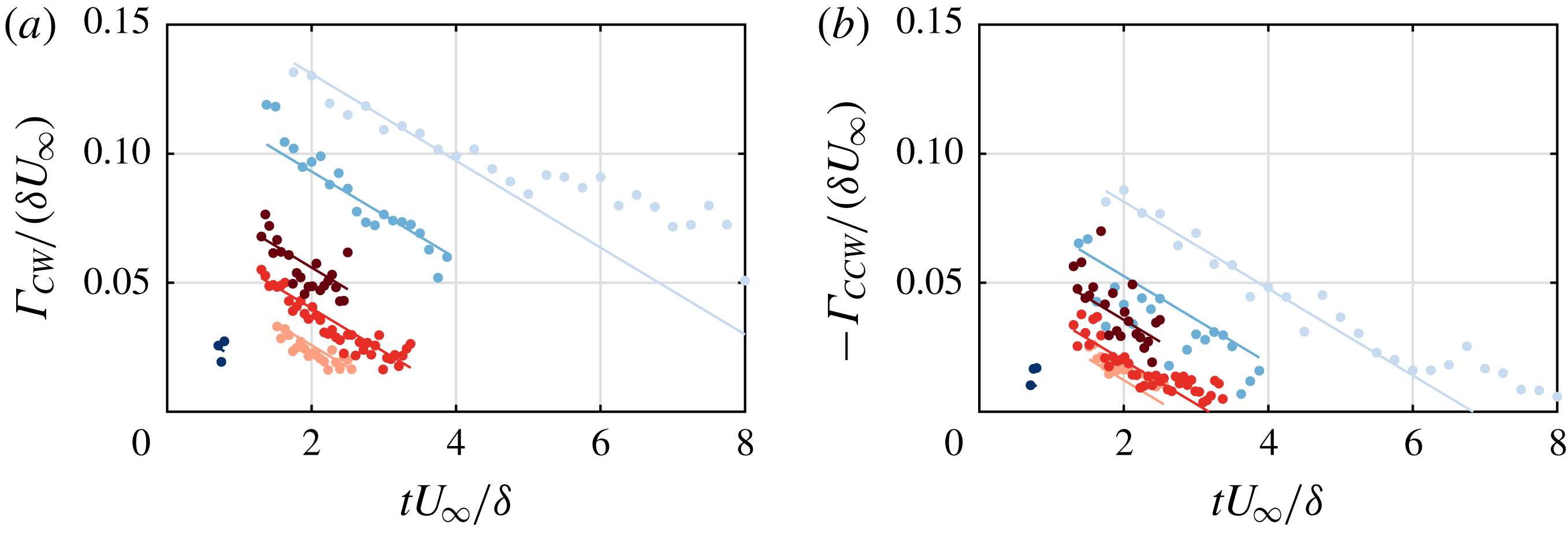
The circulation of the vortical structures decays over time. The normalized circulation of the measured cases in the present study is presented in figures 15(a) and 15(b) for the clockwise and counter-clockwise vortex respectively. A linear trend is added to the data, indicating a constant decay. This decay of circulation is incorporated in the model.
Normalized decay of circulation for (a) the clockwise vortex and (b) the counter-clockwise vortex as function of time for
 $r=0.88$
and
 $St=0.1$
,
 $0.3$
,
 $0.7$
and
 $0.9$
(darker shades of blue for increasing
 $St$
) and (b)
 $St=0.7$
and
 $r=0.45$
,
 $0.88$
and
 $1.35$
(darker shades of red for increasing
 $r$
).

3.3.3 Results of the model
As discussed above the developed model describes the evolution of a given train of input structures. The resulting strength and location of these structures can be used to study (i) the deformation of the vortical structures, (ii) the three-dimensional three-component induced velocity field and (iii) the wall-normal penetration of the structures in the cross-flow (i.e. the trajectory). Results are discussed here based on the
 $St=0.1$
,
 $r=0.88$
case.
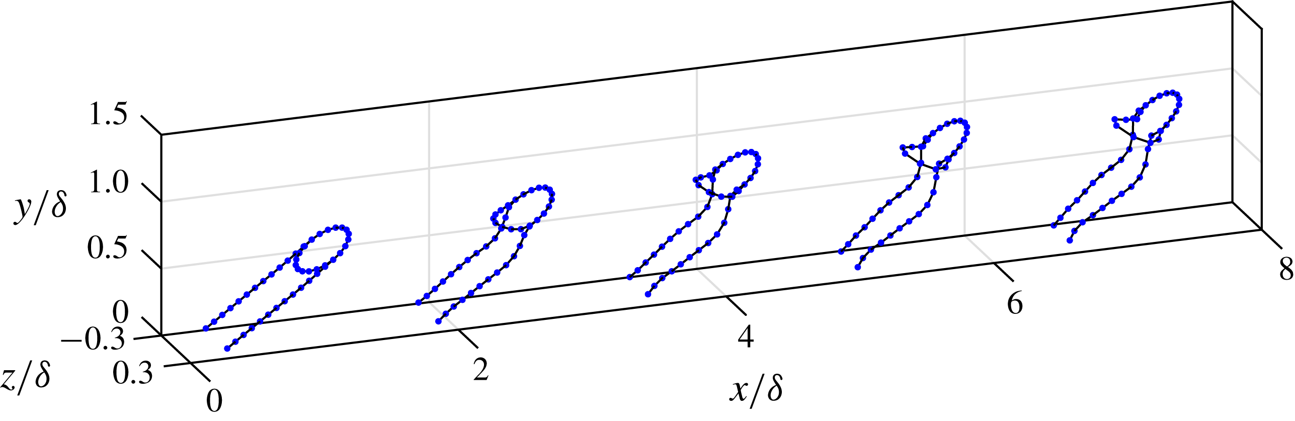
(i) An instantaneous snapshot of the vortical structures resulting from the model is presented in figure 16. The shape of the structures shows a deformation from the input geometry (around
 $x/\unicode[STIX]{x1D6FF}=1$
) to a geometry resembling the shape of the reconstructed structures as presented in figure 5(a) (around
 $x/\unicode[STIX]{x1D6FF}=7$
). The deformation of this shape indicates that the induced velocity is the driving force leading to this geometry rather than viscous effects or initial conditions.
Instantaneous result of the inviscid-flow model for
 $St=0.1$
,
 $r=0.88$
.

(ii) Given the position of vortical structures as presented in figure 16, the three components of the induced velocity can be calculated at any point
 $(x,y,z)$
using the Biot–Savart law. The velocity induced in the streamwise–wall-normal plane at the centreline of the jet (
 $z/\unicode[STIX]{x1D6FF}=0$
) is presented in figure 17. The instantaneous streamwise and wall-normal velocity components (corresponding to the position of the structures as presented in figure 16) are presented in (a) and (b), respectively. Results are qualitatively similar to the measured and reconstructed phase-locked velocity fields presented in figure 11. The time-averaged (constructed from 32 phases) streamwise and wall-normal velocity components are presented in (c) and (d) respectively. Excluding the start-up phenomena, the time-averaged velocity fields are qualitatively similar to the reconstructed velocity fields presented in figure 12(c,d) with the streamwise component dominated by a flow in opposite direction of the cross-flow and the wall-normal component dominated by a flow away from the wall. Both velocity components are strongest at the wall-normal location of the head of the vortical structure rather than the legs, indicating that the induced momentum deficit as well as up-wash are mainly driven by the vortex ring. Both components show a clear decay with streamwise distance caused by the decay of circulation of the vortical structure.
Phase-locked (a,b) and time-averaged (c,d) streamwise (a,c) and wall-normal (b,d) velocity components computed by the inviscid-flow model for the
 $St=0.1$
,
 $r=0.88$
case.

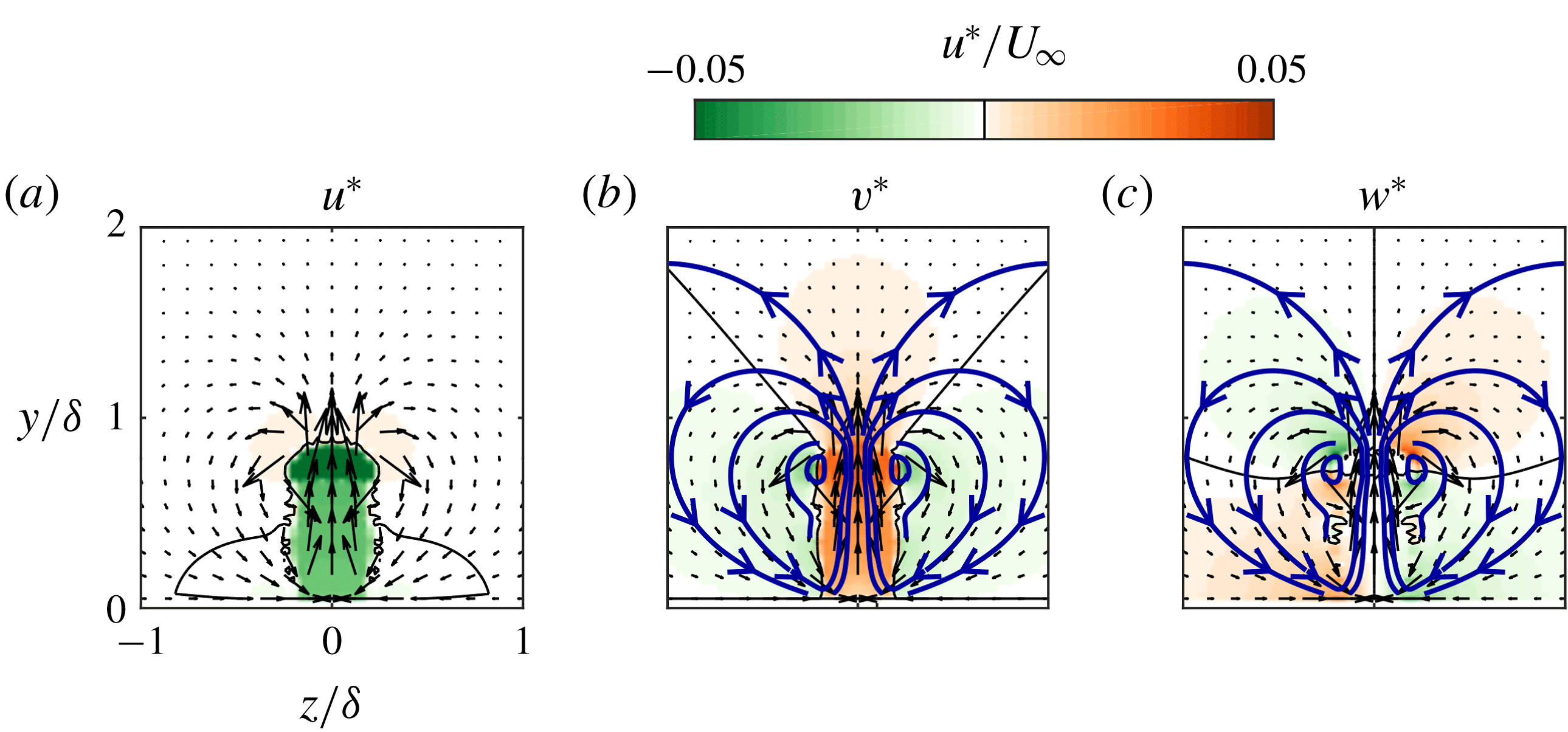
Time-averaged (a) streamwise, (b) wall-normal and (c) spanwise velocity components in the spanwise–wall-normal plane at
 $x/\unicode[STIX]{x1D6FF}=3$
computed by the inviscid-flow model for the
 $St=0.1$
,
 $r=0.88$
case. Selected streamlines are plotted in blue. Contour lines at
 $u^{\ast }/U_{\infty }=0$
are plotted in black.

For most of the present paper the velocity and the momentum-flux deficit have been considered in the streamwise–wall-normal centreline plane. Due to the nature of the flow around a vortex, the velocity components are of opposite direction inside and outside the legs of the vortical structure (see for example the schematics in figure 4). This makes it important to consider the velocity outside the structure (i.e. in off-centreline planes) as well. The inviscid-flow model enables computation of the three-dimensional three-component velocity field (as opposed to being restricted to a given measurement plane in the performed PIV experiments). The time-averaged velocity in the spanwise–wall-normal plane at
 $x/\unicode[STIX]{x1D6FF}=3$
is presented in figure 18 for the (a) streamwise, (b) wall-normal and (c) spanwise velocity components. The streamwise component (a) indicates that within the structure there is a strong negative component as seen in the centreline plane. Outside the structure (both above and to the sides) the induced velocity is slightly positive, indicating a flow in the same direction as the cross-flow. However, this component is negligible compared to the negative component and decays even further with distance from the structure. The wall-normal component (b) shows that within the structure the velocity is away from the wall, as seen in the centreline plane. In contrast, to the sides of the structure the induced velocity is towards the wall. These vertical components lead to the up-wash of low-momentum fluid at the centreline of the structures and down-wash of high-momentum fluid at the sides of the structure. The spanwise component (c) shows a velocity away from the centreline above the structure and towards the centreline below the head of the structure. Selected in-plane streamlines are overlaid on the velocity maps. These streamlines indicate a time-averaged circular motion similar to the flow around a steady counter-rotating vortex pair (also called streamwise rollers) as widely observed for steady jets in cross-flow (Mahesh Reference Mahesh2013). Large streamwise rollers have been observed both instantaneously and in time-averaged sense for synthetic jets in cross-flow by for example Van Buren et al. (Reference Van Buren, Beyar, Leong and Amitay2016a
). The time-averaged circular motion causes a net increase in streamwise momentum near the wall and around the vortical structures and a net decrease away from the wall and within the vortical structure. This increase in streamwise momentum near the wall was observed in figure 12(e) and leads to an increase in skin friction, adding to the momentum-flux deficit.
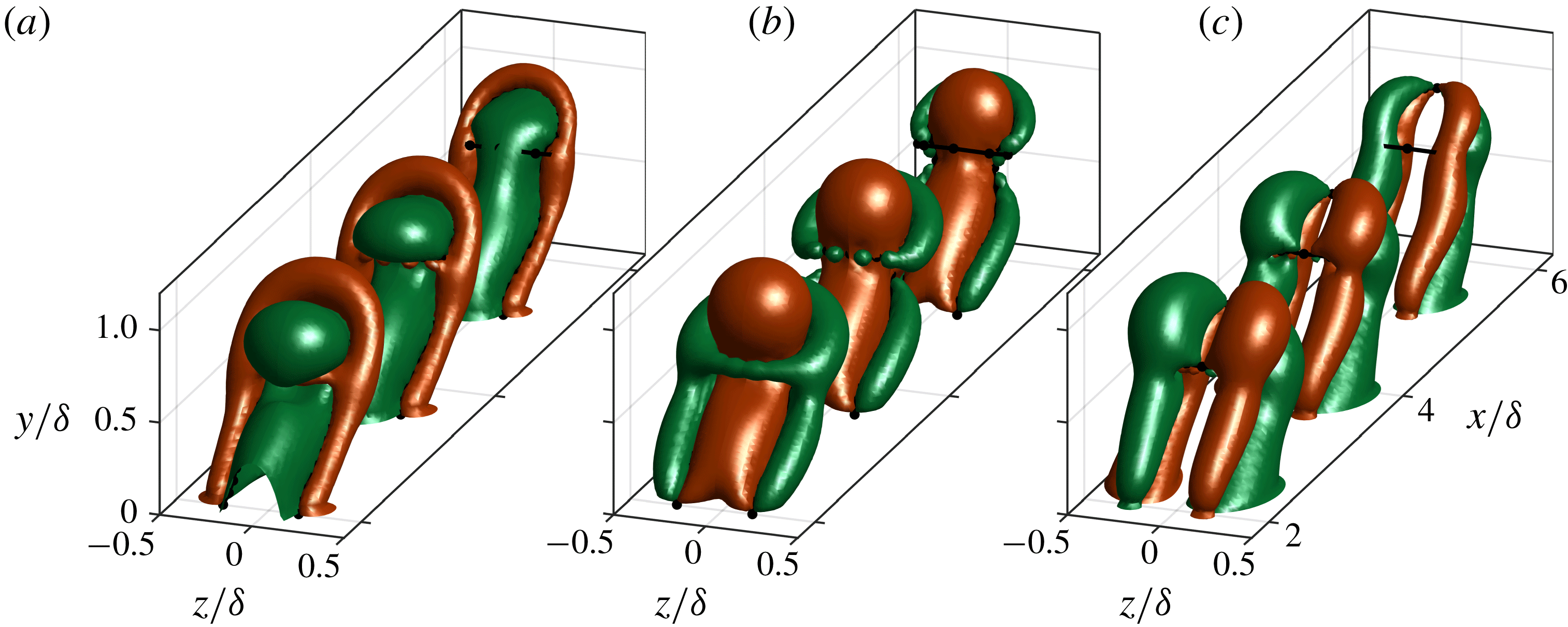
The instantaneous three-dimensional velocity field is presented in figure 19 using iso-contours of velocity at
 $u^{\ast }/U_{\infty }=\pm 0.02$
for the (a) streamwise, (b) wall-normal and (c) spanwise components respectively. These three-dimensional structures indicate the same circular motions around the vortical filaments as observed above in streamwise–wall-normal and spanwise–wall-normal planes. The dominance of the component opposite to the cross-flow as well as the component away from the wall is clearly visible in these three-dimensional representations.
Iso-contours of the instantaneous (a) streamwise, (b) wall-normal and (c) spanwise velocity components computed by the inviscid-flow model for the
 $St=0.1$
,
 $r=0.88$
case. Iso-contours indicate
 $u^{\ast }/U_{\infty }=\pm 0.02$
. Vortical filaments are indicated by black dots (nodes) and lines (segments).

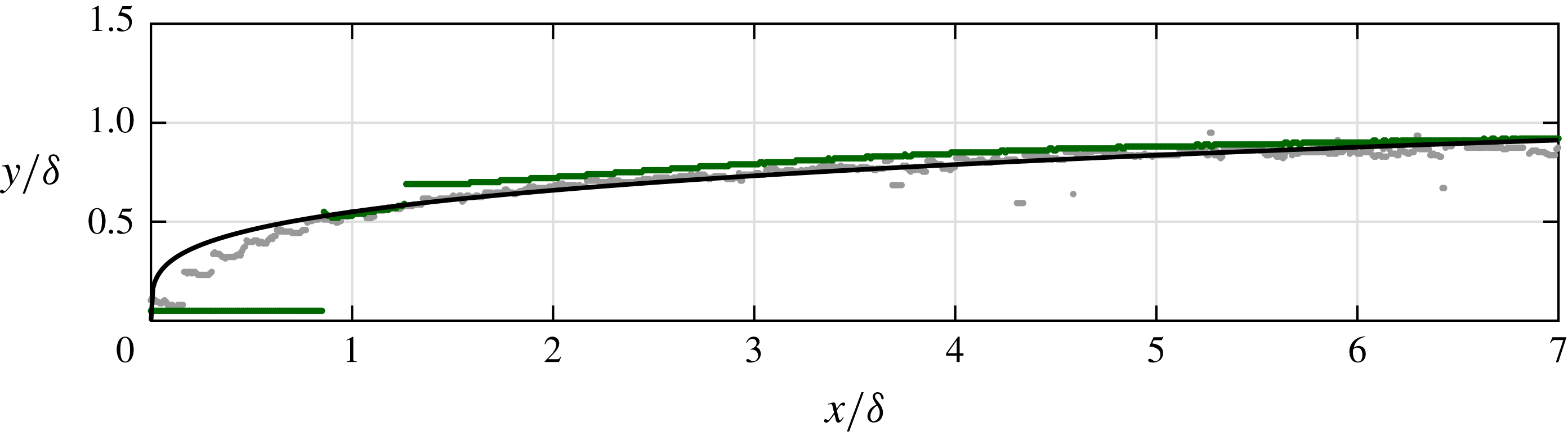
(iii) The trajectory of the jet in the model is compared to the measured trajectory for the
 $St=0.1$
,
 $r=0.88$
case in figure 20. The trajectory is defined as locations of maximum velocity deficit. Note that in the model the vortical structures are created at
 $x/\unicode[STIX]{x1D6FF}=1$
at a wall-normal height of
 $y/\unicode[STIX]{x1D6FF}=0.6$
as determined from the data. Downstream of this location the measured and modelled jet show the same trajectory. This implies that downstream of
 $x/\unicode[STIX]{x1D6FF}=1$
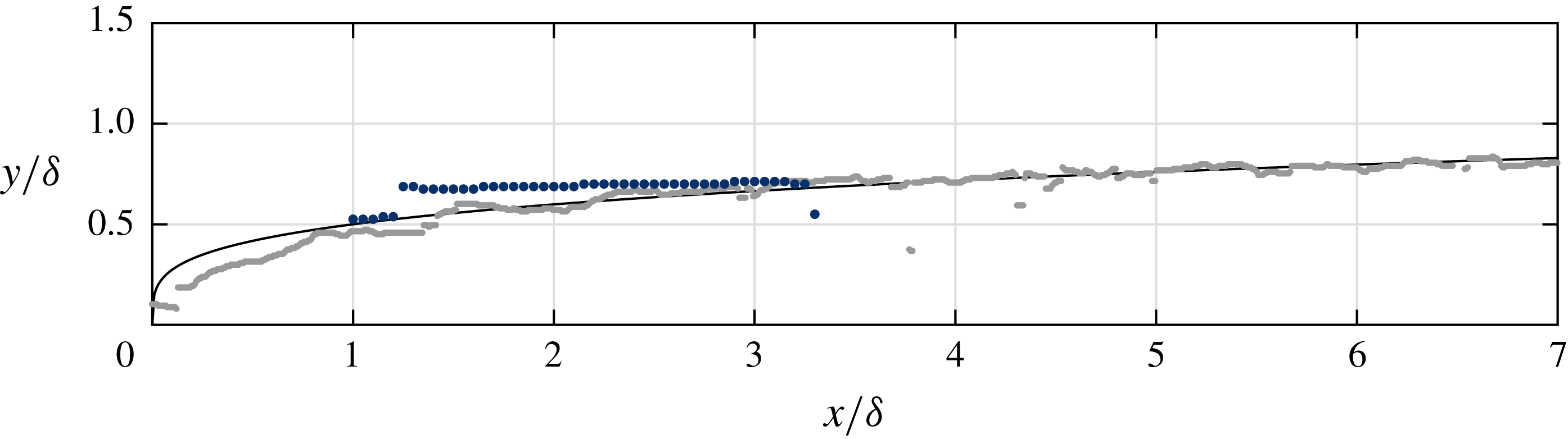
, i.e. in the far field of the jet, the trajectory is driven by the induced velocity of the vortical structures. This means that in this far field the effect of the vertical momentum created at the jet exit has disappeared. The trajectory of the jet in the far field follows a power law as indicated by the black line in figure 20. This power-law behaviour is in agreement with findings in our recent paper Berk et al. (Reference Berk, Hutchins, Marusic and Ganapathisubramani2018).
Trajectory computed by the inviscid-flow model (green dots) compared to the measured trajectory (grey dots). Each dot indicates a single streamwise grid point of either the PIV velocity field or the computed velocity field. The black line shows the power law
 $y/\unicode[STIX]{x1D6FF}=0.55(x/\unicode[STIX]{x1D6FF})^{0.26}$
.

3.3.4 Modelling parametric variations
The model is expanded to include small variations of
 $St$
and
 $r$
. Using the results computed by the model, the qualitative influence of these parameters on the trajectory is explored. As discussed above, the initial conditions for the model consist of the shape, circulation and location of the vortical structure. The initial geometry of the input structure is not varied, which limits the model to small parametric variations. The initial circulation and location of the structure are varied with respect to the baseline case (
 $St=0.1$
,
 $r=0.88$
), based on theoretical scalings with
 $St$
and
 $r$
. As discussed in § 3.2.2, the circulation of the vortical structures theoretically scales with
 $\unicode[STIX]{x1D6E4}_{0}\propto \bar{u}_{j}^{2}/f$
. When normalized using the free-stream velocity and the slot length this equals
 $\unicode[STIX]{x1D6E4}_{0}/(lU_{\infty })\propto r^{2}/St$
. This proportionality is used to vary the initial circulation with respect to the baseline case. It is assumed that the streamwise starting position of the far field does not change. Therefore, the starting position for the model is taken to be
 $x_{0}/\unicode[STIX]{x1D6FF}=1$
as used above. For the initial wall-normal position it is assumed that in the near field the jet acts like a ‘slug’ of fluid which is analogous to the concept of a stroke length
 $L=\bar{u}_{j}/f$
to describe the synthetic jet (Smith & Glezer Reference Smith and Glezer1998). This suggests that in the near field the vertical velocity scales with the mean blowing velocity
 $\bar{u}_{j}$
and the wall-normal location scales with
 $y_{0}\propto \bar{u}_{j}t_{0}$
where
 $t_{0}$
indicates the time from the onset of the jet until the structure reaches the initial position used in the model. It may be assumed that the streamwise advection velocity of the structure scales with the free-stream velocity, i.e.
 $x_{0}\propto t_{0}U_{\infty }$
, which leads to
 $y_{0}\propto \bar{u}_{j}x_{0}/U_{\infty }$
. For the initial position
 $x_{0}/\unicode[STIX]{x1D6FF}=1$
this equals
 $y_{0}/\unicode[STIX]{x1D6FF}\propto r$
. It should be noted that the variation in
 $y_{0}$
is a significant simplification. However, the results below indicate that the slope of the trajectory is independent of the wall-normal starting position.
The simplifications in the model, in combination with the invariant input geometry, limit the model to small parametric variations. This can be illustrated by trying to bridge the gap between different measured cases using the model. Starting from the
 $St=0.1$
,
 $r=0.88$
case, the input parameters are varied to represent the
 $St=0.3$
,
 $r=0.88$
case. The trajectory as computed by the model is compared to the measured trajectory for
 $St=0.3$
,
 $r=0.88$
in figure 21. The wall-normal starting position of the model is higher than in the measured data, which is an effect of the simplifications in
 $y_{0}$
. More significantly, the wall-normal penetration rate in the model is lower than for the measured data. This is assumed to be caused by (i) a difference between the circulation of the real structures and
 $\unicode[STIX]{x1D6E4}_{0}$
in the model and (ii) a difference between the geometry of the real vortical structures (which varies between cases) and the geometry of the structures in the model (which is constant between case). These differences indicate that the model cannot be used for larger parametric variations as the differences in circulation, starting position and geometry are too large.
Trajectory for
 $St=0.3$
,
 $r=0.88$
as measured (light grey dots), modelled as parametric variation around
 $St=0.1$
(dark blue dots) and as described by a power law
 $y/\unicode[STIX]{x1D6FF}=0.50(x/\unicode[STIX]{x1D6FF})^{0.26}$
(black line).

The model is used for small variations around an input case, for which the geometry of the vortical structures may be assumed similar and for which the simplifications in initial position and circulation do not lead to large errors. The model is run for variations in
 $St$
and
 $r$
around the
 $St=0.10$
,
 $r=0.88$
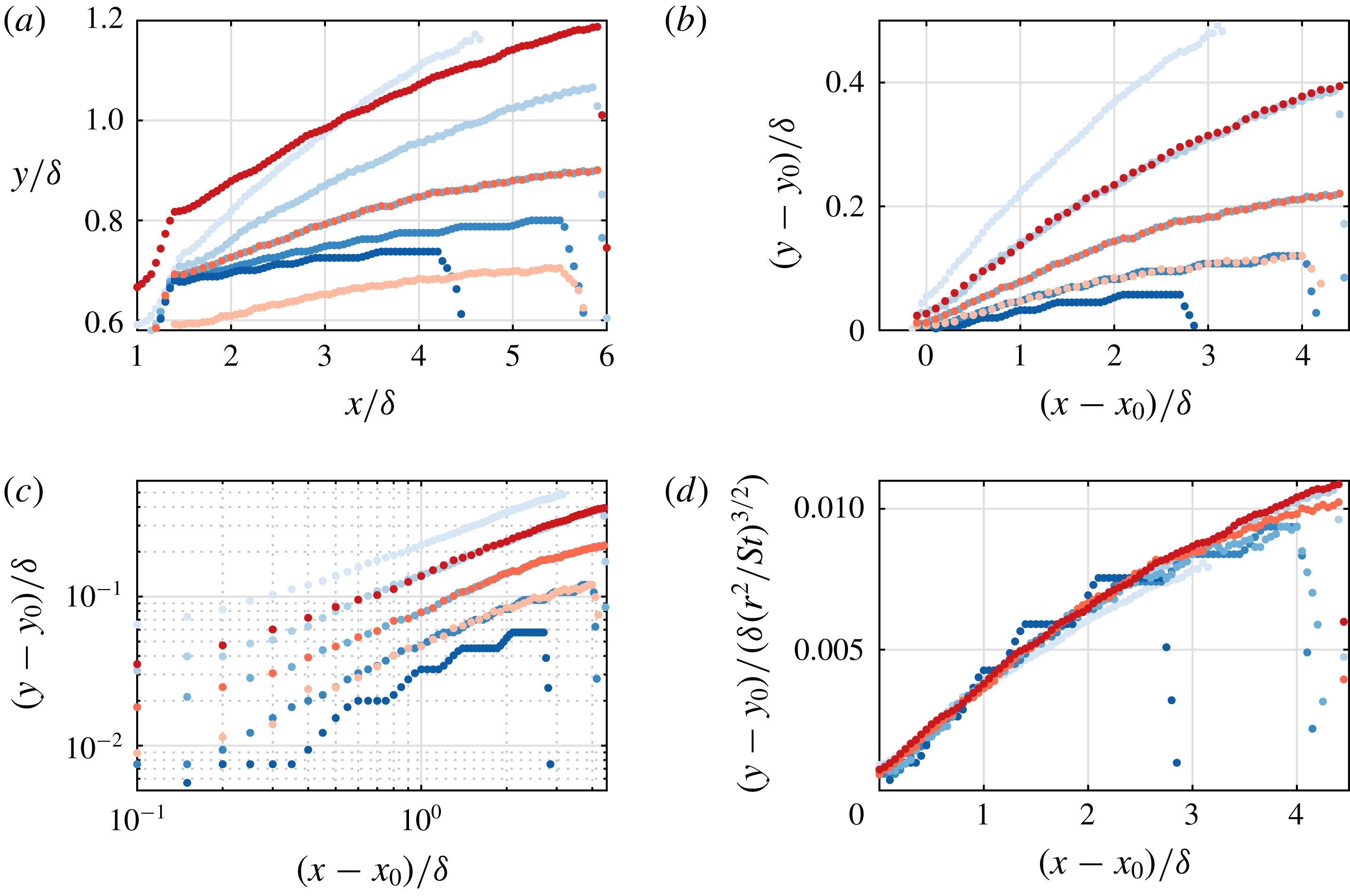
case as tabulated in table 2. Computed trajectories are presented in figure 22(a). As discussed above, the initial position (scaling with
 $y_{0}/\unicode[STIX]{x1D6FF}\propto r$
) depends only on
 $r$
. The penetration of the jet decreases for increasing
 $St$
and increases for increasing
 $r$
. The wall-normal location is highly dependent on the starting position
 $y_{0}$
. To correct for this offset, trajectories are presented relative to the starting position (
 $x_{0}$
,
 $y_{0}$
) in figure 22(b). In this relative plot it is apparent that some cases have an equal rate of penetration (i.e. the same wall-normal velocity). Overlapping cases have equal circulation (for example
 $St=0.07$
,
 $r=0.88$
and
 $St=0.10$
,
 $r=1.05$
, both with
 $\unicode[STIX]{x1D6E4}_{0}/\unicode[STIX]{x1D6E4}_{ref}$
= 1.41), indicating that the wall-normal velocity is fully driven by the circulation and independent of the distance from the wall. In the literature (e.g. Mahesh Reference Mahesh2013, Berk et al.
Reference Berk, Hutchins, Marusic and Ganapathisubramani2018), the trajectory of a (synthetic) jet in cross-flow is typically described by a power law of the form
 $$\begin{eqnarray}\frac{y}{g(\ldots \,\!)}=A\left(\frac{x}{g(\ldots \,\!)}\right)^{n},\end{eqnarray}$$
where
 $A$
and
 $n$
are constants while
 $g(\ldots \,\!)$
is a function of actuation and cross-flow parameters. When this power law is plotted on logarithmic axes, the slope equals
 $n$
while the offset is given by a function of
 $A$
and
 $g$
. Relative trajectories are presented on logarithmic axes in figure 22(c). In agreement with the literature, the constant slope across all cases indicates that the power
 $n$
is a constant. Since the wall-normal velocity is driven by circulation, it can be assumed that
 $g(\ldots \,\!)$
is a function of
 $\unicode[STIX]{x1D6E4}_{0}$
, i.e. a function of
 $r^{2}/St$
. The relative trajectories are presented with the wall-normal position normalized by
 $(r^{2}/St)^{3/2}$
in figure 22(d) (note that the exponent
 $3/2$
is determined empirically). Using this normalization, the trajectories of almost all cases are collapsed.
Trajectories computed by the inviscid-flow model as function of Strouhal number for
 $r=0.88$
and
 $St=0.05$
,
 $0.07$
,
 $0.10$
,
 $0.14$
and
 $0.20$
(darker shades of blue as
 $St$
increases) and as function of velocity ratio for
 $St=0.10$
and
 $r=0.74$
,
 $0.88$
and
 $1.05$
(darker shades of red as
 $r$
increases).

Input parameters (
 $St$
,
 $r$
) and initial conditions (
 $x_{0}/x_{ref}$
,
 $y_{0}/y_{ref}$
and
 $\unicode[STIX]{x1D6E4}_{0}/\unicode[STIX]{x1D6E4}_{ref}$
) used in the model. Reference values
 $x_{ref}$
,
 $y_{ref}$
and
 $\unicode[STIX]{x1D6E4}_{ref}$
are for the reference case
 $St=0.10$
,
 $r=0.88$
.

It should be stressed that due to the offsets in the starting positions in figure 22(d) the power law as stated in (3.5) is modified. This modification influences both the slope of the trajectories (
 $n$
), as well as the exponent (
 $3/2$
) in the normalization. The baseline case (for which the wall-normal offset is known) can be used to evaluate the exponents in the power law. As illustrated in figure 20 both the model and the experimental data follow a power law with exponent
 $n=0.26$
. Using this value, in combination with the scaling found above, the power law in (3.5) can be expressed as
 $$\begin{eqnarray}\frac{y/\unicode[STIX]{x1D6FF}}{(r^{2}St^{-1})^{a}}=A\left(\frac{x/\unicode[STIX]{x1D6FF}}{(r^{2}St^{-1})^{a}}\right)^{0.26},\end{eqnarray}$$
for an unknown exponent
 $a$
. This expression can be related to the description of the trajectory in high-Reynolds-number turbulent boundary layers as postulated in our recent paper (Berk et al.
Reference Berk, Hutchins, Marusic and Ganapathisubramani2018). For a given incoming cross-flow boundary layer and a constant orifice geometry, the trajectory in Berk et al. (Reference Berk, Hutchins, Marusic and Ganapathisubramani2018) can be expressed as
 $$\begin{eqnarray}\frac{y/\unicode[STIX]{x1D6FF}}{r^{1.26}St^{-0.56}}=B\left(\frac{x/\unicode[STIX]{x1D6FF}}{r^{1.26}St^{-0.56}}\right)^{0.32}.\end{eqnarray}$$
This expression agrees with the scaling of the trajectories predicted by our model (for
 $a\approx 0.6$
in (3.6)). This indicates that variations of the trajectory in the far field are driven by the circulation and self-induced velocity of the vortical structures. The exponent found in the present study (0.26 in (3.6)) is slightly lower than the exponent found in Berk et al. (Reference Berk, Hutchins, Marusic and Ganapathisubramani2018) (0.32). This may be caused by the relatively low Strouhal number regime investigated here, which causes independent behaviour of subsequent vortical structures, leading to decreased penetration compared to interacting structures observed in Berk et al. (Reference Berk, Hutchins, Marusic and Ganapathisubramani2018).
4 Conclusions
The interaction of a synthetic jet with a cross-flow leads to a momentum-flux deficit in the cross-flow. In the literature this deficit is often ascribed to either viscous blockage of the cross-flow by the synthetic jet or by the up-wash of low-momentum fluid. The present paper has introduced and discussed a third source of the momentum-flux deficit: a velocity induced in the direction opposite to the cross-flow by the vortical structures created by the synthetic jet.
It is shown that the momentum deficit created by viscous blockage recovers quickly downstream of the jet exit. It is hypothesized that the main influence of up-wash is the accompanying down-wash of high-momentum fluid, increasing the effect of skin friction which acts as a momentum sink.
The effect of vortex-induced velocity is determined by reconstructing the vortical structures created by the synthetic jet using measured velocity fields. The velocity induced by these reconstructed structures is calculated by applying the Biot–Savart law to these measured structures. This induced velocity shows large qualitative and quantitative similarity to the measured velocity fields, indicating that the driving source of velocity fluctuations is the induced velocity, rather than blockage or up-wash. It is shown that for low Strouhal numbers the momentum deficit downstream of the blockage wake is entirely caused by the velocity induced in the direction opposite of the cross-flow. This implies that the increase in skin friction is negligible for these low Strouhal numbers, which can be explained by the large separation between subsequent structures, enabling the flow to recover between structures. For higher Strouhal numbers a constant offset between the measured and induced momentum deficit is observed, suggesting a constant increase in skin friction. The momentum-flux deficit starts to decrease for high Strouhal numbers, caused by the approach of the formation criterion, meaning that part of the synthetic jet is re-ingested during the suction phase of the jet, decreasing its strength. The momentum deficit increases with velocity ratio, caused by the increasing strength of vortical structures created by the jet. It is shown that the increase in skin friction is relatively constant with velocity ratio.
An inviscid-flow model is developed in which the evolution of a train of vortical structures of given geometry and circulation is computed. Results of the model are presented for a single case equal to one of the measured cases. It is shown that the geometry of the vortical structure in the model deforms from the simplified input structure to a shape resembling the measured vortical filaments. This suggests that the shape of the vortical structures is driven by the induced velocity rather than viscous effects or initial conditions. The inviscid-flow model is able to reconstruct three-dimensional three-component velocity fields. Velocity fields computed by the model in planes equal to the measurement planes show a great (qualitative) similarity of the measurements to the inviscid computations. The instantaneous velocity field is dominated by a component opposite to the cross-flow and away from the wall within the vortical structure. Outside the vortical structure a weaker component is present in the direction of the cross-flow and towards the wall. The same is true in the time-averaged velocity field. Finally, the far-field trajectory of the vortical structures in the inviscid-flow model is equal to the measured trajectory of the synthetic jet, indicating that in this far field the trajectory is driven by self-induced velocity rather than by initial conditions or viscous effects. Small parametric variations in the model indicate that changes in the trajectory are driven by the circulation of the created vortical structures. Based on these parametric variations an expression for the trajectory of synthetic jets is derived that agrees well with experimental results in the literature.
The present paper has presented evidence that the velocity induced by vortical structures created by a synthetic jet plays an important role in the velocity field around the jet. In the far field of the jet this induced velocity is the main contributor to the momentum deficit in the cross-flow as well as the development (both the trajectory and structure) of the jet.
Acknowledgements
We acknowledge the financial support from the EPSRC (grant no. EP/L006383/1) and European Research Council (grant agreement no. 277472). The inviscid-flow model used and all data supporting this study are openly available from the University of Southampton repository at http://dx.doi.org/10.5258/SOTON/D0859.
Supplementary material
Supplementary material is available at https://doi.org/10.1017/jfm.2019.279.