1 Introduction
The displacement of one fluid by another in a quasi-two-dimensional geometry is common to a wide range of natural and industrial systems. In some systems, the evolving interfaces between the two fluids can maintain a smooth circular or planar shape, but in others they can develop fingering instabilities and consequently evolve complex patterns.
A large class of interfacial-stability problems, known as viscous fingering, involves flows that are dominated by shear, typically due to the traction imposed by confining solid boundaries. In these shear-dominated flows in a uniform gap, it is established that the interface is stable when the displacing fluid is more viscous, either in a system of Newtonian fluids that obeys Darcy’s law and the pressure field is Laplacian (Saffman & Taylor Reference Saffman and Taylor1958; Wooding & Morelseytoux Reference Wooding and Morelseytoux1976; Paterson Reference Paterson1981; Homsy Reference Homsy1987; Bhaskar et al. Reference Bhaskar, Garik, Turner, Bradley, Bansil, Stanley and Lamont1992; Cardoso & Woods Reference Cardoso and Woods1995; Coumou et al. Reference Coumou, Driesner, Geiger, Heinrich and Matthai2006; Jha, Cueto-Felgueroso & Juanes Reference Jha, Cueto-Felgueroso and Juanes2011; Zhao, MacMinn & Juanes Reference Zhao, MacMinn and Juanes2016; Rabbani et al. Reference Rabbani, Or, Liu, Lai, Lu, Datta, Stone and Shokri2018), or when at least one of the fluids is complex and the pressure field is no longer Laplacian (Lemaire et al. Reference Lemaire, Levitz, Daccord and Vandamme1991; Zhao & Maher Reference Zhao and Maher1993; Kondic, Shelley & Palffy-Muhoray Reference Kondic, Shelley and Palffy-Muhoray1998; Coussot Reference Coussot1999; Lindner, Bonn & Meunier Reference Lindner, Bonn and Meunier2000a ; Lindner, Coussot & Bonn Reference Lindner, Coussot and Bonn2000b ; Azaiez & Singh Reference Azaiez and Singh2002; Callan-Jones, Joanny & Prost Reference Callan-Jones, Joanny and Prost2008). A more general statement is that the interface is stable when the displacing fluid is less mobile than the displaced fluid, where mobility is the ratio of permeability and viscosity. The physical requirement for instability in these systems is that the magnitude of the driving pressure gradient is larger in the displaced fluid than in the displacing fluid, which can be hydrostatic rather than dynamic (Kowal & Worster Reference Kowal and Worster2019). Instability can be suppressed or triggered by specifying a non-uniform gap between the confining boundaries (Al-Housseiny, Tsai & Stone Reference Al-Housseiny, Tsai and Stone2012), which affects the driving pressure gradients. In addition, non-monotonic mobility profiles in confined miscible flows can lead to reverse fingering, in which the displaced fluid fingers through the displacing fluid more readily than vice versa (Manickam & Homsy Reference Manickam and Homsy1994).
The flow geometry also affects the stability of confined shear-dominated flows. Particularly, for a constant-flux source, Newtonian flows in a circular geometry tend to be more stable than flows in a linear geometry (e.g. Paterson Reference Paterson1981) because the velocity of circular interfaces declines with time and circumferential stretching tends to push perturbation to lower wavenumbers. A priori, such flow configurations may appear prone to Saffman–Taylor instability if a single fluid phase of strain-rate-softening fluid propagates axisymmetrically. This is because the radial decline of the dominant strain-rate component leads to monotonically increasing viscosity, or declining mobility, with radius. This implies that any ring of fluid within such flows is like an interface between an inner less-viscous fluid and an outer more-viscous fluid. Although there is no viscosity jump across such fluid rings and they behave as rather smeared interfaces, one might anticipate that instability could still occur as it does in miscible Newtonian fluids (Paterson Reference Paterson1985; Manickam & Homsy Reference Manickam and Homsy1993; Holloway & de Bruyn Reference Holloway and de Bruyn2005). However, viscous fingering in radially spreading, strain-rate-softening fluids has not been observed thus far. Similar axisymmetric flows of strain-rate-softening fluids were studied using viscous gravity currents that propagate into low-viscosity fluids over a horizontal substrate. Such flows have mixed boundary conditions of no slip along their base and no stress along their free surface due to the absence of confinement. Here too, despite a radially increasing viscosity within the strain-rate-softening displacing fluids, no fingering was observed (Sayag & Worster Reference Sayag and Worster2013).
In another class of problems, which forms the focus of this paper, the fluids have free top and bottom surfaces along which traction is negligible and the resulting circular flow is dominated by extension rather than by shear. In this case, evidence shows that unique finger-like patterns can arise with the fluid appearing to be torn apart when the displacing fluid is strain-rate softening. For example, ice shelves deform like strain-rate-softening fluids (Glen Reference Glen1955) under negligible traction, as they spread over the ocean. When ice shelves are free from lateral confinement, finger-like patterns can emerge normal to the shelf front, separated by deep rifts, reminiscent of tears (rips) that cut through the entire ice thickness (Hughes Reference Hughes1983; Doake & Vaughan Reference Doake and Vaughan1991; Bassis et al. Reference Bassis, Fricker, Coleman and Minster2008; Borstad, McGrath & Pope Reference Borstad, McGrath and Pope2017). Similarly, tear-like patterns emerge when pastes squeezed by parallel disks emerge outside of the rim of the disks into a region that is unconfined where no external stress is applied (Mascia et al. Reference Mascia, Patel, Rough, Martin and Wilson2006; Roussel, Lanos & Toutou Reference Roussel, Lanos and Toutou2006). The formation of these patterns is potentially related to the migration of the liquid phase within the pastes as they spread. In contrast, the interface remains stable in similar flows of Newtonian displacing fluids, such as viscous gravity currents that spread radially under no traction (Pegler & Worster Reference Pegler and Worster2012).
In this Part 1 of the study we extend Sayag & Worster (Reference Sayag and Worster2013) by allowing a thin film of strain-rate-softening fluid to propagate with the absence of any traction along its boundaries, thereby forming an extensionally dominated flow. We trace the evolution of the fluid–fluid interface in time and analyse its wavenumber decomposition. We then analyse the pattern in which the dominant wavenumber of the interface evolves and how that pattern depends on the main experimental control parameter, the source mass flux. In Part 2 of this study (Sayag & Worster Reference Sayag and Worster2019) we focus on a theoretical investigation of the instability reported here.
2 Experimental observations
2.1 Experimental set-up
We generated extensional flows experimentally by discharging a thin layer of viscous fluid into a bath filled with low-viscosity but denser fluid. This way traction on the viscous fluid was reduced substantially, allowing extensional stresses to dominate. The experimental apparatus (figure 1) consisted of a transparent bath of
 $1\times 1~\text{m}^{2}$
filled with low-viscosity, transparent salt solution to a depth of 15 mm. At the centre of the bath and attached to its bottom we placed a conical section made of transparent polydimethylsiloxane (PDMS), which had a trapezoidal cross-section (figure 1
b) with dimensions 15 mm height, 10 cm top base diameter and 18 cm bottom base diameter. The displacing complex fluid was driven from a container by a peristaltic pump at constant flux (
 $1\lesssim Q\lesssim 14$
)
 $\text{g}~\text{s}^{-1}$
, which was measured with an accuracy of
 $\pm 0.05~\text{g}~\text{s}^{-1}$
using a computer connected to a digital balance that supported the container. From the pump the fluid was discharged axisymmetrically through a tube, 10 mm in diameter, over the centre of the top base of the conical section. The fluid continued to propagate under gravity over the conical section and beyond, displacing the ambient salt solution. The propagation of the interface was imaged using a digital SLR camera in plan view from the bottom of the bath through a 45
 $^{\circ }$
mirror at a rate of one frame every 2–6 s, depending on the source flux.
(a) Schematic diagram of the experimental apparatus to generate extensional flows. The region where the flow evolves (dotted rectangular) is expanded in (b). (b, top) Schematic side view of the flow region, showing the polymer solution (blue) propagating radially over the conic plate and into a bath of salt solution (cyan), resulting in a no-stress interface at the surface and the base of the displacing fluid. (b, bottom) An image showing the camera plan view of the flow at a stage where the front of the polymer solution developed four fingers. The vertical dashed lines mark the radius
 $r_{G}$
, which is where the fluid–fluid interface intersects with the conical section.

To keep the level of the ambient fluid in the tank fixed as the complex fluid was intruding, we used a secondary pump controlled by an optical feedback circuit. Specifically, a red laser beam was emitted through the ambient fluid and underwent total internal reflection from the ambient-fluid free surface towards an optical sensor. A rise in the level of the ambient fluid shifted the beam trajectory from the sensor and consequently operated the pump that drained excess fluid, until the beam resumed intersection with the sensor, thereby turning the pump off. This way we managed to keep the level of the ambient fluid fixed to within a 0.1 mm accuracy.
The complex fluid consisted of Xanthan gum (Jungbunzlauer) dissolved in distilled water (1 % in weight), having density
 ${\approx}1.02~\text{g}~\text{cm}^{-3}$
. Xanthan is a semirigid and high-molecular-weight polysaccharide produced by the Xanthomonas campestris bacterium (Lapasin Reference Lapasin1995). To prepare the solution we used a laboratory mixer to form a smooth vortex in the centre of a 3 l beaker containing the distilled water. The Xanthan powder (from a single batch) was then spread into the centre of the vortex through a sieve to disperse powder aggregates, thereby allowing faster polymer hydration. Next, we added a couple of millilitres of blue dye and maintained the mixing for one hour at the maximum speed possible so long as air bubbles did not intrude into the fluid. Then the solution was left for the next 24 h in a closed container to allow full hydration of the polymer. This way we obtained an agglomerate-free and bubble-free Xanthan solution.
The rheology of Xanthan gum solutions of
 ${\sim}1\,\%$
concentration has been studied extensively in various flow configurations. Under steady-shear flow, such solutions behave as a power-law, shear-thinning fluid with exponent
 ${\approx}6$
(Sayag & Worster Reference Sayag and Worster2013) for the solution we used, although other measurements find that it can vary between
 ${\approx}5$
(Martin-Alfonso et al.
Reference Martin-Alfonso, Cuadri, Berta and Stading2018) and
 ${\approx}7$
(Song, Kim & Chang Reference Song, Kim and Chang2006a
) (we define shear thinning with exponents larger than 1). At low shear rates there are indications of bounded shear viscosity at more dilute polymer concentrations than 1 % (Wyatt & Liberatore Reference Wyatt and Liberatore2009; Jaishankar & McKinley Reference Jaishankar and McKinley2014; Allouche et al.
Reference Allouche, Botton, Henry, Millet, Usha and Hadid2015) with a zero strain-rate viscosity of over
 $10^{6}$
times that of water at
 $25\,^{\circ }\text{C}$
at shear rates lower than
 $10^{-3}~\text{s}^{-1}$
(Jaishankar & McKinley Reference Jaishankar and McKinley2014), and possibly the presence of yield stress (e.g. Herschel-Bulkley fluid, Song et al.
Reference Song, Kim and Chang2006a
). These solutions also exhibit elastic properties such as primary normal-stress difference over a wide range of strain rates (Jaishankar & McKinley Reference Jaishankar and McKinley2014), and a relaxation time of
 $\unicode[STIX]{x1D706}\approx 0.1~\text{s}^{-1}$
(Stokes et al.
Reference Stokes, Macakova, Chojnicka-Paszun, de Kruif and de Jongh2011). In oscillatory-shear flow, the storage modulus of such suspensions is 2–4 times larger than the loss modulus in frequencies ranging between 0.01 and
 $100~\text{rad}~\text{s}^{-1}$
(Song, Kuk & Chang Reference Song, Kuk and Chang2006b
). In uniaxial extensional flows, Xanthan solutions exhibit strain hardening (Stelter & Brenn Reference Stelter and Brenn2002; Stelter et al.
Reference Stelter, Brenn, Yarin, Singh and Durst2002), as well as strain-rate softening of the extensional viscosity (extensional thinning) with an exponent of
 ${\approx}3$
(Jones, Walters & Williams Reference Jones, Walters and Williams1987; Ferguson, Walters & Wolff Reference Ferguson, Walters and Wolff1990; Martin-Alfonso et al.
Reference Martin-Alfonso, Cuadri, Berta and Stading2018), while the behaviour at extensional rates lower than approximately
 $0.5~\text{s}^{-1}$
is not known. The ratio of extensional to shear viscosity (Trouton ratio) of such solutions grows with the strain rate, reaching approximately 30 at strain rate of
 $1~\text{s}^{-1}$
(Jones et al.
Reference Jones, Walters and Williams1987; Martin-Alfonso et al.
Reference Martin-Alfonso, Cuadri, Berta and Stading2018), but at lower strain rates it drops and is expected to converge to the Newtonian value of 3, as typical of polymeric solutions (Bird, Armstrong & Hassager Reference Bird, Armstrong and Hassager1987). Therefore, at the higher end of the strain rate, such Xanthan solutions have a more significant elastic deformation, while viscous deformation becomes more significant at the lower end.
The ambient fluid consisted of sodium chloride solution with density
 ${\approx}1.181\,\text{g}\,\text{cm}^{-3}$
, and therefore denser than the Xanthan gum solution. This combination of fluids resulted in the formation of a region in the flow where the Xanthan solution was propagating over the denser ambient fluid, which was significantly less viscous and consequently applied negligible traction.
2.2 Evolution of the interface
We performed a range of experiments in which we varied the source flux
 $Q$
of the polymer solution, while keeping fixed the level and density of the ambient salt solution, and the concentration of the polymer solution (table 1).
The source flux
 $Q$
(
 $\pm 0.05~\text{g}~\text{s}^{-1}$
uncertainty) that was specified in each experiment and the resulting measured grounding-line position
 $r_{G}$
and the fluid thickness
 $h_{G}$
at the grounding line. In all the experiments the polymer solution consisted of 1 % Xanthan gum and the density of the salt solution was
 $\unicode[STIX]{x1D70C}=1.181~\text{g}~\text{cm}^{-3}$
.

Once discharged from the tube, the gravity-driven polymer solution propagated axisymmetrically over the truncated cone surrounded by a deep layer of denser and low-viscosity salt solution. When the circular fluid front intruded into the ambient salt solution, as it advanced along the sloping section of the cone, buoyancy forces due to the surrounding denser fluid caused it to detach from the substrate and float (figure 1
b, top). This way, a circular contact line (grounding line) was formed at radius
 $r_{G}>5~\text{cm}$
over the slope of the cone, separating between an inner region (
 $r<r_{G}$
) where no-slip basal conditions were applied to the polymer solution, and an outer region (
 $r>r_{G}$
) where no-stress basal conditions were applied to the polymer solution. Within a short transient the grounding line advanced down the slope of the substrate and reached a steady position that was maintained for all
 $t>0$
. We discovered that the leading front of the displacing polymer solution split into a number of tongues in the vicinity of
 $r_{G}$
, which moved as solid blocks similar to the movement of floating ice tongues (e.g. Holdsworth Reference Holdsworth1983) or of foam under wall slip (Lindner et al.
Reference Lindner, Coussot and Bonn2000b
). The region between the tongues resembled fractures with sharp tips near
 $r_{G}$
, reminiscent of fracture tips (figure 1
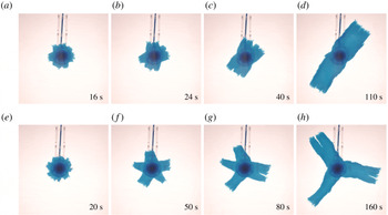
b, bottom). As the tongues grew longer, some of those tips were advected with the flow and, as they did, the space between the tongues closed by the joining of adjacent tongues into wider ones. Consequently, the number of tongues declined with time (figure 2 and supplementary movies are available at https://doi.org/10.1017/jfm.2019.777). Such an inverse cascade of the number of tongues also appears to characterise patterns in squeezed pastes (Mascia et al.
Reference Mascia, Patel, Rough, Martin and Wilson2006), in fractured thin elastic plates (Vermorel, Vandenberghe & Villermaux Reference Vermorel, Vandenberghe and Villermaux2010; Vandenberghe, Vermorel & Villermaux Reference Vandenberghe, Vermorel and Villermaux2013) and in melt transport (Spiegelman, Kelemen & Aharonov Reference Spiegelman, Kelemen and Aharonov2001). However, the breakdown of the circular symmetry that we report is in sharp contrast with similar flows that involved Newtonian displacing fluids (Pegler & Worster Reference Pegler and Worster2012), in which the fluid–fluid interface remained circular.
Snapshots (plan view) from two experiments with source flux (a–d)
 $Q=3.90\pm 0.05~\text{g}~\text{s}^{-1}$
and (e–h)
 $Q=2.64\pm 0.05~\text{g}~\text{s}^{-1}$
, showing the evolution of the fluid–fluid interface. The injected complex fluid is coloured blue, and the ambient less viscous, denser fluid as well as the conical substrate are transparent. Time is measured with respect to the instant when the interface reached the grounding-line position. The Fourier modes of each interface in (e–h) are shown in figure 5(b).

Snapshots (plan view) from the experiment with source flux
 $Q=2.64\pm 0.05~\text{g}~\text{s}^{-1}$
tracing the evolution of the interface as it transits the steady grounding-line position at
 $t=0$
. The injected polymer solution is coloured blue, and the ambient denser fluid as well as the conical substrate are transparent. The origin is the centre of the tube outlet (

 $\cdots \cdots$
, green) in each of the previous panels, normalised by the intensity of the background (ambient fluid). The grounding-line position at each time is the local minimum of the intensity between 5 cm (the top edge of the substrate slope,
 $\cdots \cdots$
) and
 ${\sim}6~\text{cm}$
(▴), where (- - -, red) marks the grounding-line steady position.

Fourier decomposition of the fluid–fluid interface: examples from three different experiments (
 $Q=2.64,1.36,1.37\pm 0.05~\text{g}~\text{s}^{-1}$
), showing snapshots of the traced interface (——) and the results of the regression (——, red) of part of the interface (
 $r\leqslant 2.5\,r_{G}$
) to the Fourier series (2.1).

2.3 Analysis of the results
Having image sequences of the experimental results, we first determine the grounding-line steady position
 $r_{G}$
and the instant when the front crossed that position for each experiment. We define the origin
 $r=0$
at the centre of the feeding tube using snapshots taken before the fluid was discharged. We also identify the rim of the larger base of the PDMS substrate (figure 3
a) and use its known diameter (18 cm) to convert from pixels to dimensional length. Then we identify the position of the grounding line using the intensity of the light transmitted through the polymer solution (figure 3
f). Specifically, the part of the fluid that spreads along the higher base of the conical section from the nozzle is relatively thick and appears as a dark disk that becomes radially brighter towards the edge of that top base. Near that edge and just before the fluid intrusion into the salt solution, the fluid thickness is minimal and appears as a thin ring of brighter colour (figure 3
e), with a corresponding local maximum in the light intensity at radius 5 cm (figure 3
f). Across that ring, the polymer solution intrudes into the ambient fluid along the substrate slope (figure 1
b), so it becomes thicker and consequently darker with radius, as also implied from the corresponding decline in the light intensity. Further down along the substrate slope, another sharp transition occurs into a brighter region, which implies that the fluid layer has gone through a sudden thinning. Such abrupt thinning that coincides with a local minimum in the light intensity (figure 3
f) is due to the detachment of the fluid layer from the slope of the substrate (figure 1
b, top). Therefore, we identified that local minimum in intensity, which varies with azimuth by less than
 $\pm 2$
mm, with the position of the grounding line. We follow the propagation of the grounding line along the slope from the time it is formed very close to the top base and until it reaches a steady position within a short transient (figure 3
f). Upon detachment of the polymer solution, the basal friction drops abruptly and substantially and the fluid layer flows as a plug (no vertical shear), becoming a pure extensional flow with principal axes along the radial and azimuthal directions resulting in horizontal stretching, and perpendicular to the direction of flow resulting in vertical thinning (e.g. Robison, Huppert & Worster Reference Robison, Huppert and Worster2010; Pegler & Worster Reference Pegler and Worster2013). Having the steady grounding-line position and knowing the substrate geometry, we calculate the fluid thickness at that position,
 $h_{G}$
, assuming that the fluid is floating (table 1). In addition we define
 $t=0$
at the instant when the fluid front reaches the steady position of the grounding line (figure 3).
The sharp colour contrast between the polymer solution and the salt solution allowed a straightforward tracing of the fluid–fluid interface
 $r_{N}(\unicode[STIX]{x1D703},t)$
as a function of time (figure 4) using image-processing tools. Applying a fast Fourier transform to the raw interface leads to inconsistent results, particularly when the interface roughness is substantial, having sections with multiple fracture-like elements that enhance the interface length in these parts disproportionally (e.g. figure 4
c). To avoid such complications we first truncate at each instant the part of the interface having
 $r>2.5r_{G}$
and then fit to the residual traced interface a Fourier series of the form
 $$\begin{eqnarray}f(t)=a_{0}(t)+\displaystyle \mathop{\sum }_{k=1}^{N}a_{k}(t)\sin (k\unicode[STIX]{x1D703}+\unicode[STIX]{x1D719}_{k}(t)),\end{eqnarray}$$
where the amplitudes
 $a_{0\ldots N}$
and the phases
 $\unicode[STIX]{x1D719}_{1\ldots N}$
are the fitted parameters (figure 4). We chose
 $N=30$
noticing that a larger value does not affect the amplitude distribution
 $a_{k}(t)$
in a measurable way. In addition, the value of the truncation radius was robust and was used for all experiments. We applied this routine to each experimental snapshot and got a time series of the wavenumber amplitude distribution (figure 5
a,b). Then, we normalised the amplitude distribution at each instant with the maximal amplitude at that instant, obtaining the normalised amplitude distribution of the different Fourier modes for the whole duration of the experiment (figure 5
c). For clarity, that distribution is a smoothed (interpolated) version of the original discrete distribution (appendix A). This wavenumber–amplitude distribution, which is typical for a wide range of experiments, shows that the initial circular front (
 $t<0$
) first develops a high-wavenumber pattern (
 $0<t<20~\text{s}$
) that then declines progressively and monotonically through a descending set of dominating wavenumbers to a finite
 $k=3$
dominating wavenumber. This reduction of the dominating wavenumber is reflected in the experiment through the repeated merging of adjacent fingers into wider ones (figure 2).
(a) The traced fluid–fluid interface at times
 $t=20$
, 50, 80, 160 s (thick curves) in the experiment with
 $Q=2.64\pm 0.05~\text{g}~\text{s}^{-1}$
(figure 2
e–h), with the grounding line marked in (——, green). (b) Amplitude distribution (lines) of the dominating Fourier wavenumbers that compose each of the interfaces in (a) (colours match) obtained by fitting a Fourier series of the front
 $r_{N}(\unicode[STIX]{x1D703},t)$
(♢ marking the maximum amplitude in each case). (c) Time evolution of the amplitude distributions (interpolated) normalised by the maximum amplitude at each time, where darker colour represents modes with higher amplitudes (discrete version is shown in appendix A). Vertical gridlines mark the distributions at times that match (by colour) those shown in (b).

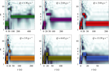
Time evolution of the normalised amplitude of the Fourier modes (dark, smoothed) that comprise the fluid–fluid interfaces for experiments with source flux in the range
 $1.3\lesssim Q\lesssim 13.4\pm 0.05~\text{g}~\text{s}^{-1}$
. The maximal amplitudes at each instant are highlighted with colour patches. In each panel, the horizontal gridline marks the average wavelength after the initial cascade of wavenumbers.

We repeated the same analysis procedure for all of the experiments with varying source flux
 $Q$
(table 1), and generated the corresponding wavenumber–amplitude distributions (figure 6, 7). The evolution of the interface is reflected in the evolution of the dominant wavenumbers – those modes that have maximum amplitude at each instant (figure 8). In these experiments we find that the wavenumber evolution at early time has a different pattern compared to late time. At early time, the patterns that emerged from the initial circular front had high dominating wavenumber, which gradually cascaded into a lower dominating wavenumber at increasingly growing transition times. This behaviour characterised all experiments, and quantitatively the rate of the cascade (transition time to lower wavenumbers) and the lowest wavenumber that the pattern converged to was strongly dependent on the source flux
 $Q$
. At later times, after the initial cascade to the lower wavenumber, the interface evolved in two distinguished patterns depending on the input flux. In the higher-flux regime (
 $Q\gtrsim 1.37~\text{g}~\text{s}^{-1}$
), the asymptotic pattern remained in the lowest wavenumber of the initial cascade. That lowest wavenumber declined with the source flux (figure 8
a). In the lower-flux regime (
 $Q\lesssim 1.37~\text{g}~\text{s}^{-1}$
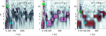
), the dominating wavenumber did not settle on a well-defined fixed value, rather, it changed stochastically within a finite band of wavenumbers (figure 8
b). This appears to imply that, while instantaneously the pattern has an integer dominant wavenumber, on average the system can asymptotically settle on a fractional wavenumber.
Time evolution of the normalised amplitude of the Fourier modes (dark, smoothed) that comprise the experimental fronts for experiments with source flux in the range
 $Q=0.73,1.37,1.38\pm 0.05~\text{g}~\text{s}^{-1}$
, in which the dominant wavenumber varies stochastically after the initial wavenumber cascade. The maximal amplitudes at each instant are highlighted with colour patches. In each panel the ○, green marks the instant when the pattern had a maximum dominant wavenumber. The ○, cyan marks the instant when the pattern had the lowest wavenumber at the termination of the wavenumber cascade, beyond which the dominant wavenumber evolved stochastically. In each panel, the horizontal gridline marks the average wavenumber after the initial cascade of wavenumbers.

3 Discussion
The apparent stochastic evolution of the dominant wavenumber in the lower-flux experiments (figure 8
b) motivates us to evaluate a time-averaged asymptotic wavenumber. To do this we identified in each experiment the time when the initial wavenumber cascade terminated. This was done by first finding the instant when the pattern had the maximal wavenumber. The instant that followed at which the pattern had the minimal wavenumber was defined as the end of the wavenumber cascade phase (e.g. figure 7). The time-average dominant wavenumber
 $\unicode[STIX]{x1D705}$
is defined as the time average of the dominant wavenumbers in the interval from that latter instant onwards. Those lower-flux experiments in which the dominant wavenumber evolved stochastically after the initial cascade (figure 8
b) had a fractional time-average wavenumber and a standard deviation of about one wavenumber (figure 9
a), whereas the higher-flux experiments (figure 8
a) had zero standard deviation. In addition, the time-average wavenumbers decline monotonically with the source flux
 $Q$
(figure 9
a).
The dependence on
 $Q$
of the time-averaged dominant wavenumber and of the transition times to lower wavenumbers may be partially scaled away with an appropriate
 $Q$
-dependent time scale. One way to define a time scale using the measured quantities is to consider the flow at
 $r=r_{G}$
. When the flow is quasi-steady, the grounding-line position is steady and so is the thickness of the free surface for
 $r<r_{G}$
. Therefore, conservation of mass implies that from that stage on, the total volume flux across a circle of radius
 $r_{G}$
is equivalent to
 $Q$
. Therefore, at the grounding-line position,
 $Q=2\unicode[STIX]{x03C0}r_{G}h_{G}u_{G}$
, where
 $u_{G}$
is the radial velocity at
 $r_{G}$
. In addition, the scale of
 $u_{G}$
can be written in terms of
 $u_{G}=r_{G}/{\mathcal{T}}$
, where
 ${\mathcal{T}}$
is a characteristic time scale of the flow. Substituting this relation in the expression for the flux we find that the characteristic time scale is
 $$\begin{eqnarray}{\mathcal{T}}={\displaystyle \frac{2\unicode[STIX]{x03C0}r_{G}^{2}h_{G}}{Q}}.\end{eqnarray}$$
Using the measurements in table 1, we evaluated the characteristic time scale (3.1) in each experiment and used it to normalise the time evolution of the dominant wavenumber. We applied this to the experimental results that behaved regularly and not stochastically in the long-time limit (figure 8
a) and found that the measurements collapse into a narrower region (figure 9
b). This demonstrates that the patterns we observe in experiments with different mass fluxes share common features when the rate of the flow represented by the flux is scaled away. Particularly, it may imply that in the non-stochastic cases the wavenumber cascade could end up at the lowest possible wavenumber for any source flux
 $Q$
, and that the associated time scale could grow like
 $1/Q$
, as implied from (3.1). The lowest wavenumber may be
 $k=2$
, although in the experiment with the highest
 $Q=13.39~\text{g}~\text{s}^{-1}$
we found that one tongue was approximately 30 % thicker than the other, and that the angle between their axes of propagation was less than
 $180^{\circ }$
. This may represent an intermediate pattern before a transition to
 $k=1$
at higher flux. Experiments with
 $Q>3~\text{g}~\text{s}^{-1}$
have all reached
 $k=2$
by the time
 $t\simeq {\mathcal{T}}$
(figure 9
b), and those experiments that terminated at higher wavenumbers lasted no longer than
 $t\simeq 3{\mathcal{T}}$
. Therefore, it may be that
 ${\mathcal{T}}$
represents a damping time scale and that within less than
 ${\approx}10{\mathcal{T}}$
any flows would converge to wavenumber
 $k=2$
and possibly less.
The dominant wavenumbers (maximum instantaneous amplitude) versus time and source flux
 $Q$
in
 $\text{g}~\text{s}^{-1}$
, corresponding to the experiments in which (a) the late-time evolution of the dominant wavenumber converged to a fixed value (figure 6), and in which (b) the dominant wavenumber changed stochastically (figure 7).

The Xanthan solution that we used has a viscoelastic deformation in principle. The relative role of elastic compared to viscous deformation can be estimated by the ratio of the fluid elastic-relaxation time
 $\unicode[STIX]{x1D706}$
and the characteristic rate of flow
 ${\mathcal{T}}$
, as represented by the Deborah number
 $De=\unicode[STIX]{x1D706}/{\mathcal{T}}$
. Having
 $\unicode[STIX]{x1D706}\approx 0.1~\text{s}$
(Stokes et al.
Reference Stokes, Macakova, Chojnicka-Paszun, de Kruif and de Jongh2011), the maximal Debora number in the experiments we report (
 $0.01~\text{s}^{-1}<1/{\mathcal{T}}<0.07~\text{s}^{-1}$
) that corresponds to the smallest
 ${\mathcal{T}}$
, is
 $De\approx 0.007$
. This suggests that the characteristic time scale of the flow in all of the experiments is much longer than the time scale of the fluid elastic relaxation, implying that in the flow we consider elastic effects are weaker than viscous deformation. As indicated in § 2.1, more direct measurements of the relative strength of elasticity under extension at rates similar to those in the experiments we report are absent. The known decline of the Trouton ratio with the decline of the rate of deformation (Jones et al.
Reference Jones, Walters and Williams1987; Martin-Alfonso et al.
Reference Martin-Alfonso, Cuadri, Berta and Stading2018) implies that the relative strength of elasticity drops at smaller strain rates, but measurements at extensional rates lower than
 $0.5~\text{s}^{-1}$
are absent in the literature. Similarly, in other flow configurations the relative strength of elasticity drops as the rate of deformation declines. For example, in simple-shear flow the ratio of the normal-stress difference and shear stress (stress ratio, Bird et al.
Reference Bird, Armstrong and Hassager1987) drops from 5 at a shear rate of
 $1~\text{s}^{-1}$
to 1 at a shear rates of
 $10^{-2}~\text{s}^{-1}$
(Jaishankar & McKinley Reference Jaishankar and McKinley2014). In oscillatory-shear flow the ratio of the storage to loss moduli drops from 3 at a shear rate of
 $1~\text{s}^{-1}$
to approximately 2 at a shear rate of
 $10^{-2}~\text{s}^{-1}$
(Song et al.
Reference Song, Kuk and Chang2006b
). Despite the decline of the elastic strength with the decline of rate in these examples, as in extensional flows, at low shear rates (
 ${\approx}0.01~\text{s}^{-1}$
) elasticity can be comparable to the viscous deformation in simple shear or even larger in oscillatory shear. However, these values may not necessarily indicate the specific Trouton ratio in the extensional flow that we study, which differs substantially from both oscillatory and simple shear flows.
The flow of the polymer solution from the inner, shear-dominated region across
 $r_{G}$
to the free-slip region is associated with a Reynolds number. Considering the grounding-line position, we find that
 $Re=Q\unicode[STIX]{x1D70C}/2\unicode[STIX]{x03C0}r_{G}\unicode[STIX]{x1D707}$
. To estimate an upper bound for
 $Re$
we use
 $Q\sim 10$
and the viscosity associated with the largest strain rate (
 $0.1~\text{s}^{-1}$
)
 $\unicode[STIX]{x1D707}\sim 10^{2}~\text{Pa}~\text{s}$
, resulting in
 $Re\lesssim 10^{-3}$
.
Although the polymer solution is in contact with both the salt solution and air, we expect that the impact of surface tension on the dynamics of the front is weak, having a secondary or higher-order contribution owing to two major reasons. Firstly, the density ratio of the two solutions implies that nearly 80 % of the displacing front of the polymer solution is submerged in the salt solution, yet the two solutions are nearly miscible as their surface tensions differ only by approximately 5 % (surface tension of 1 % Xanthan gum solution
 ${\sim}0.0825~\text{N}~\text{m}^{-1}$
at
 ${\sim}25\,^{\circ }\text{C}$
(Muthamizhi et al.
Reference Muthamizhi, Kalaichelvi, Powar and Jaishree2014), and the corresponding value of our sodium chloride solution is
 ${\sim}0.0785~\text{N}~\text{m}^{-1}$
(Bzdek et al.
Reference Bzdek, Power, Simpson, Reid and Royall2016)). Secondly, deforming the highly viscous and possibly unyielded polymer solution at the front requires larger external stresses than could be provided by surface tension. The low traction applied to the floating tongues combined with the strain-rate-softening property of the polymer solution leads to high fluid viscosity (at least
 ${\sim}100~\text{Pa}~\text{s}$
, Sayag & Worster (Reference Sayag and Worster2013)) in most of the tongues and particularly along the front, such that the fluid in those regions appears unyielded throughout the whole experiment. Such immobility of the polymer solution is reflected in the vertically flat (figure 1
b) and thick fluid front (similar to
 $h_{G}$
, table 1), in contrast to the wedge-like front when the displacing fluid is Newtonian (Pegler & Worster Reference Pegler and Worster2013).
(a) The dependence of the average dominant wavenumber on the source flux. The time-averaged dominant wavenumber (coloured ♢ corresponding to the colours in figure 8) is computed for the time after the initial wavenumber cascade to a minimal value. A
 $\pm 1$
standard deviation of the dominant wavenumber distribution is marked by the error bars. Experiments with non-zero standard deviation (♢, red) are those shown in figure 8(b). Inset shows one example of the dominant wavenumber distribution for the experiment with
 $Q=0.73~\text{g}~\text{s}^{-1}$
, and the fitted Gaussian distribution used to compute the average and standard deviation. (b) Non-dimensional time evolution of the dominant Fourier modes that the front is comprised of, for a range of source fluxes
 $1.3\gtrsim Q\gtrsim 13.4~\text{g}~\text{s}^{-1}$
corresponding to those in figure 8(a).

4 Conclusions
In this experimental study we have shown that the interface between a strain-rate-softening fluid that displaces a lower-viscosity fluid can become unstable when friction is nearly negligible along the path of the flow. Our experiments using polymer solutions that deform under nearly free-slip conditions showed that the initially circular interfaces become unstable, evolving rectangular-shaped fingers with rough edges reminiscent of tears in solid material. Tracing the dominant wavenumber in the instantaneous Fourier decomposition as a function of time, we find that the evolution of the interface consists of two primary stages: in the initial wavenumber cascade stage the interface ruptured into multiple fingers that gradually grew and merged into a smaller number of wider fingers; in the second stage, the pattern evolved either regularly or stochastically depending on the discharge rate. At higher discharge rates the pattern remained in the lowest-wavenumber form, which corresponds to a constant number of fingers whose length continuously grow. At lower discharge rates the pattern evolved within a small band of wavenumbers in a stochastic form, which corresponds to the repeated emergence of new fingers followed by their merging to existing longer fingers. In both cases, we found that the time-averaged dominant wavenumber that the evolving pattern converged to in that stage declined with the source flux. The transition time to lower wavenumbers in the initial cascade declined with the source flux as well.
The instability that we find seems strongly reliant on both the free-slip conditions and the strain-rate-softening property of the displacing fluid, and possibly of the circular geometry of the flow. Such conditions characterise other natural and man-made systems such as when non-Newtonian pastes are squeezed out of a confining geometry (Mascia et al. Reference Mascia, Patel, Rough, Martin and Wilson2006) and when glacier ice creeps over the ocean (Walker et al. Reference Walker, Bassis, Fricker and Czerwinski2013). Therefore, this study may help to understand the evolution of these systems.
In the second part of this study (Sayag & Worster Reference Sayag and Worster2019) we investigate theoretically the early-time evolution of the circular interface into tongues and the wavenumber cascade. Specifically, we analyse the linear stability of an axisymmetric base flow and thereby identify that the instability relies on the divergent nature of the flow and is allowed by the absence of boundary friction and by the strain-rate-softening property of the fluid.
Acknowledgements
We thank Jungbunzlauer for providing the Xanthan gum; R.S. thanks SIDEER and BIDR in Ben-Gurion University, Israel, for financial support, and DAMTP, University of Cambridge, UK, where some of this research took place. This research was supported by the Israel Science Foundation (grant no. 1368/16).
Supplementary movies
Supplementary movies are available at https://doi.org/10.1017/jfm.2019.777.
Appendix. The discrete amplitude distribution
For the purpose of clearer graphical representation of the dominant wavenumbers, diagrams that show the evolution of the amplitude distribution of wavenumbers (figures 5 c, 6, 7, 8 and 9 b) are smoothed through a linear interpolation. At each instant the amplitude distribution of wavenumbers is discrete (figure 10) and the log scale representation of the wavenumber axis results in relatively stretched patches of the lower wavenumbers in these diagrams. Whether discrete of smoothed, the vertical thickness of such patches in these diagrams is a graphical artefact, while the meaningful values of amplitude are only those that correspond to integer wavenumbers.
Comparison of the discrete and interpolated time evolution of the normalised amplitude distributions. Panel (a) (identical to figure 5
c) is the interpolated version of panel (b) that shows a discrete distribution in which
 $k$
is integer.