1. Introduction
Buoyancy-driven turbulence is encountered in a broad range of fields, such as inertial confinement, supernovae explosions, volcanic or lake eruptions (Woods Reference Woods2010), mixing in unstable atmospheric layers and upper ocean (Peltier & Caulfield Reference Peltier and Caulfield2003) or in engineering applications as diverse as combustion, ventilation (Linden Reference Linden1999), fire propagation or oil extraction. Most of the investigations on this generic form of turbulence have focused on Rayleigh–Taylor (RT) turbulence in the unconfined situation where turbulent statistics are inherently time-dependent (except under special circumstances, e.g. Chung & Pullin (Reference Chung and Pullin2010)) and inhomogeneous in the direction of acceleration. Thanks to modern experimental (Dalziel, Linden & Youngs Reference Dalziel, Linden and Youngs1999; Ramaprabhu & Andrews Reference Ramaprabhu and Andrews2004; Banerjee, Kraft & Andrews Reference Banerjee, Kraft and Andrews2010) and computational (Ristorcelli & Clark Reference Ristorcelli and Clark2004; Livescu & Ristorcelli Reference Livescu and Ristorcelli2007, Reference Livescu and Ristorcelli2008) techniques, several fundamental processes at work in RT turbulence have been studied in detail and are now better understood.
In parallel, a research stream aimed at investigating buoyancy-induced mixing in long pipes and channels has developed throughout the last decade. Most of it focused on the vertical case in which the RT turbulence phenomenology combines with confinement effects. While the width of the mixed layer is known to grow quadratically in time during the nonlinear stages of the instability in the unconfined configuration, the confined case exhibits very different evolutions. Since the lateral size of the large-scale structures is constrained, this growth is approximately governed by a diffusive process, so that the mixed layer evolves as the square root of time when the turbulent Reynolds number is low enough (Debacq et al. Reference Debacq, Fanguet, Hulin, Salin and Perrin2001, Reference Debacq, Hulin, Salin, Perrin and Hinch2003). At higher Reynolds number, mixing length arguments and experiments in tall channels with a square cross-section rather suggest a growth with a two-fifth power of time (Dalziel et al. Reference Dalziel, Patterson, Caulfield and Coomaraswamy2008), an evolution confirmed by a hierarchy of one-dimensional models and large-scale computations (Lawrie & Dalziel Reference Lawrie and Dalziel2011a ,Reference Lawrie and Dalziel b ). Several other investigations inspired by issues related to Rayleigh–Bénard turbulence aimed at detailing the flow structure, using either miscible fluids of different densities in a long cylindrical tube (Cholemari & Arakeri Reference Cholemari and Arakeri2009) or differential heating between the top and bottom plates of a long cell with a square cross-section (Gibert et al. Reference Gibert, Pabiou, Tisserand, Gertjerenken, Castaing and Chillà2009; Tisserand et al. Reference Tisserand, Creyssels, Gibert, Castaing and Chillà2010). These studies, which made extensive use of particle image velocimetry (PIV), provided evidence for the existence of long plumes or ‘channels’ of heavy (cold) and light (hot) fluid. In particular, thanks to conditional averaging, the latter two revealed that the flow exhibits an S-shaped ‘mean’ velocity profile during long transients separated by randomly distributed reversals. The plume-like structures were found to be of central importance in the mixing process and flow dynamics, which contrasts with the conclusions of Dalziel et al. (Reference Dalziel, Patterson, Caulfield and Coomaraswamy2008) who, by means of PIV, observed the large-scale structures involved in the growth of the mixed layer looking rather as ‘billows’ with a characteristic size in every direction of the order of the channel width. The experiments by Cholemari & Arakeri (Reference Cholemari and Arakeri2009) and Gibert et al. (Reference Gibert, Pabiou, Tisserand, Gertjerenken, Castaing and Chillà2009), as well as the recent computations by Schmidt et al. (Reference Schmidt, Calzavarini, Lohse, Toschi and Verzicco2012) in a tall cylindrical Rayleigh–Bénard cell with an imposed axial temperature gradient, all exhibit the inertial (or ‘ultimate’) scaling where the Nusselt and turbulent Péclet numbers vary as the square root of the Rayleigh number, i.e. the flow statistics do not depend on the molecular diffusivity.
Another series of studies focused on the same problem in long tilted pipes and channels. For a given set of fluid properties and low-turbulent-Reynolds-number conditions, the mean density evolution was again found to follow a diffusive behaviour with an equivalent diffusivity increasing strongly with the tilt angle,
 ${\it\Theta}$
, up to a maximum. Beyond that critical angle, the transverse mixing decreases dramatically, since the light and heavy fluids tend to segregate under the effect of the transverse (stabilizing) buoyancy force (Séon et al.
Reference Séon, Hulin, Salin, Perrin and Hinch2004). Similarly, the front velocity of the two currents increases with
 ${\it\Theta}$
when the pipe is close to vertical whereas it decreases with the tilt angle at large
 ${\it\Theta}$
, exhibiting a clear ‘plateau’ corresponding to a balance between inertial and gravitational effects at intermediate angles (Séon et al.
Reference Séon, Hulin, Salin, Perrin and Hinch2005; Hallez & Magnaudet Reference Hallez and Magnaudet2008). At low-to-moderate Reynolds numbers, the effective diffusivity and front velocity were shown to decrease as the inverse of the three-half and three-quarter powers of the Reynolds number, respectively (Séon et al.
Reference Séon, Znaien, Perrin, Hinch, Salin and Hulin2007). The local characteristics of the turbulent field, especially the distribution of the variance of velocity fluctuations and that of the turbulent shear stress, started to be explored, both experimentally (using PIV) and computationally (with the present code), by Znaien et al. (Reference Znaien, Hallez, Moisy, Magnaudet, Hulin, Salin and Hinch2009). This study revealed that the near-wall region plays little role in the streamwise mean momentum transfer and showed existence of a four-roll mean secondary flow, the generation mechanism and scaling of which were elucidated by Hallez & Magnaudet (Reference Hallez and Magnaudet2009). Subsequent measurements by Znaien, Moisy & Hulin (Reference Znaien, Moisy and Hulin2011) revealed that, with large enough density contrasts and Reynolds numbers and small enough
 ${\it\Theta}$
, the mean velocity and all second-order moments including the variance of density fluctuations are stationary, although the mean density profile keeps on evolving. Last, Rayleigh–Bénard convection in a long inclined cell was recently considered by Riediger et al. (Reference Riediger, Tisserand, Seychelles, Castaing and Chillà2013) who, by recording the variations of the mean streamwise temperature gradient with the injected power, were able to identify several distinct flow regimes. In particular, they found ‘hard’ turbulence (for which the above ‘ultimate’ scaling holds) to occur for
 ${\it\Theta}\leqslant 20^{\circ }$
at large enough Rayleigh numbers, followed by ‘soft’ turbulence (for which the Nusselt number varies as the square of the Rayleigh number) at larger
 ${\it\Theta}$
. For
 ${\it\Theta}\leqslant 20^{\circ }$
, the corresponding mean velocity and shear stress profiles are similar to those of Znaien et al. (Reference Znaien, Hallez, Moisy, Magnaudet, Hulin, Salin and Hinch2009), and the smaller
 ${\it\Theta}$
the lower the critical Rayleigh number required to reach the ‘hard’ regime. New data by the same group in the range
 $5^{\circ }\leqslant {\it\Theta}\leqslant 20^{\circ }$
(Salort et al.
Reference Salort, Riedinger, Rusaouen, Tisserand, Seychelles, Castaing and Chillà2013) were interpreted in the light of a mixing length model, but the observed
 ${\it\Theta}$
-dependence of the mean velocity profile could only be recovered by altering the usual time scale of Prandtl’s original model (i.e. the inverse of the mean shear) with contributions resulting from both the stabilizing and destabilizing buoyancy components.
Odier et al. (Reference Odier, Chen, Rivera and Ecke2009) and Odier, Chen & Ecke (Reference Odier, Chen and Ecke2012) considered a different but related configuration in which an upflowing pressure-driven turbulent light current is confined in between a heavier fluid initially at rest and an upper inclined plate. Using jointly PIV and planar laser-induced fluorescence, they determined the crosswise shear stress and density flux induced by the entrainment process that takes place at the interface. Results indicate that, in this situation where the two buoyancy components are stabilizing, both quantities may be related to the mean shear and mean density gradient via an almost constant mixing length, the value of which was found to scale with the Corrsin length scale to be introduced later.
According to the above review, most available studies in confined geometries focused on the global mixing efficiency and merely characterized it through the temporal evolution of the cross-sectional average density profile. Some of the most recent ones employed PIV to investigate the instantaneous flow field and the large-scale turbulent statistics in the vertical midplane of the channel or pipe, providing mean velocity and shear stress profiles. However none of them explored the complete three-dimensional structure of the velocity and density fields which is of importance in the mixing process, as emphasized by the discovery of the mean secondary flow in the circular pipe configuration (Znaien et al. Reference Znaien, Hallez, Moisy, Magnaudet, Hulin, Salin and Hinch2009). Also, apart from those by Odier et al. (Reference Odier, Chen, Rivera and Ecke2009, Reference Odier, Chen and Ecke2012), no joint measurement of the velocity and scalar fields has been reported so far. Finally, only mean streamwise momentum balances and overall scalar balances have been examined. Hence, compared with canonical pressure-driven flows in channels and pipes, for which extensive statistics are available, the present knowledge of confined buoyancy-driven turbulent flows appears to be still in its infancy. The same is true with respect to homogeneous stably stratified sheared turbulence which has been the subject of many detailed experimental and computational investigations (e.g. Chung & Matheou Reference Chung and Matheou2012 and references therein), but also with respect to unconfined RT turbulence for which a substantial amount of statistics and energy budgets is now available thanks to recent experiments (Banerjee et al. Reference Banerjee, Kraft and Andrews2010) and extensive computations (Cabot & Zhou Reference Cabot and Zhou2013).
Consequently, the purpose of the present study is to better document the specificities of this class of flows by examining various statistical moments and approximate budgets for first- and second-order statistical quantities resulting from a numerical simulation of the low-Reynolds-number buoyancy-driven turbulent flow in a long pipe with
 ${\it\Theta}=15^{\circ }$
. This computation may be considered as the counterpart of the experiments reported by Znaien et al. (Reference Znaien, Hallez, Moisy, Magnaudet, Hulin, Salin and Hinch2009, Reference Znaien, Moisy and Hulin2011) at this particular angle, since all dynamical and geometrical parameters, including the pipe aspect ratio, are identical; detailed comparisons between experimental first- and second-order large-scale velocity statistics and some of the present numerical predictions may be found in the former paper. The only noticeable difference between the experimental and numerical set-ups lies in the mechanism that drives the small-scale scalar mixing, since we replace the small but non-zero molecular diffusion of the real system by some effect of the numerical scheme to be described below.
The structure of the paper is as follows. Section 2 describes the physical problem, the averaging procedure and the computational approach. A grid convergence study is provided in appendix A to show that the selected grid allows all significant scales of the velocity field to be correctly captured. Section 3 presents the large-scale first- and second-order statistics of the velocity and scalar (i.e. density) fields. The mean momentum and scalar balances and their implications on the crosswise shear stress and scalar flux are discussed in § 4; a rigorous derivation of these balances is provided in appendix B. Section 5 focuses on the characteristic length scales of the flow and the anisotropy they reveal. Various aspects of the energetics of the fluctuating velocity and scalar fields are discussed in § 6 with a particular focus on the production, turbulent transport and confinement mechanisms that control the corresponding variances, and on the influence of the crosswise buoyancy component on the spatial distribution of the crosswise shear stress and scalar flux. An original algebraic model incorporating destabilizing and stabilizing buoyancy effects is introduced in appendix C to relate the various components of the diffusivity tensor to those of the Reynolds stress tensor. A turbulent diffusivity and an eddy viscosity are computed for the crosswise scalar flux and shear stress, respectively, and the validity of the Reynolds analogy is assessed. Section 7 summarizes the main findings and compares some of the most typical statistics of the present flow with those of several well-documented flows of particular relevance.
2. Statement of the problem and computational strategy
2.1. The physical problem
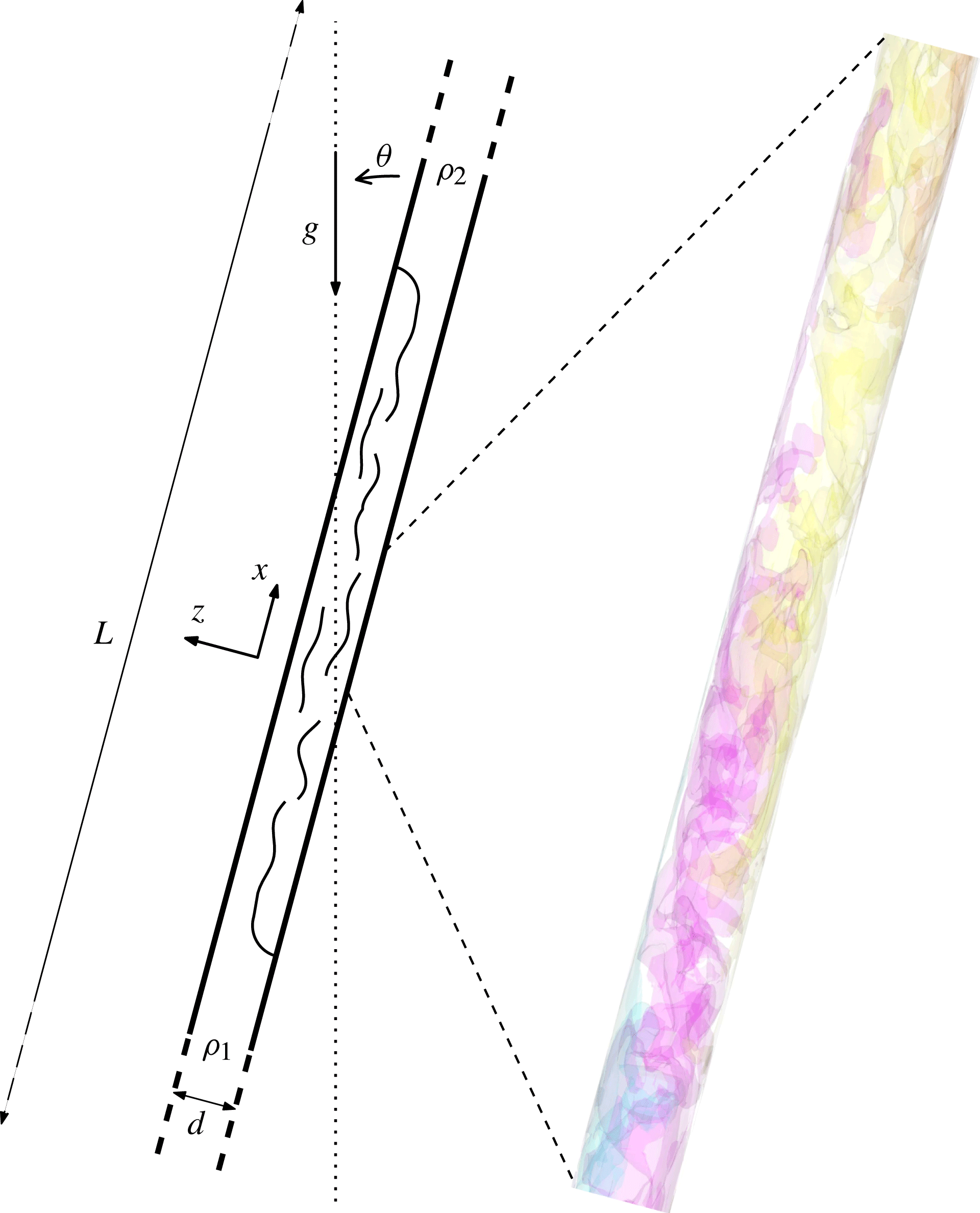
We consider an incompressible buoyancy-driven turbulent flow taking place in a long circular pipe of length
 $L$
, diameter
 $d$
, inclined at an angle
 ${\it\Theta}$
from vertical (figure 1). The Boussinesq approximation is assumed to hold. The pipe is filled with two perfectly miscible, Newtonian viscous fluids having densities
 ${\it\rho}_{1}$
and
 ${\it\rho}_{2}~({\it\rho}_{2}>{\it\rho}_{1})$
and the same kinematic viscosity,
 ${\it\nu}$
. Their small but non-zero molecular diffusivity is not explicitly taken into account; the way the small-scale scalar mixing is achieved is discussed in the next subsection. In the initial state, the light (respectively heavy) fluid occupies the lower (respectively higher) half of the pipe and the sharp interface that separates the two fluids is perpendicular to its axis. Subsequently, the two fluids mix and the local density
 ${\it\rho}$
of the mixture is related to the local volume fraction (which will generally be referred to as the ‘concentration’)
 $C$
of the heavy fluid through
 $$\begin{eqnarray}{\it\rho}=C{\it\rho}_{2}+(1-C){\it\rho}_{1}={\it\rho}_{0}[1+2\mathit{At}(C-1/2)],\end{eqnarray}$$
with
 ${\it\rho}_{0}=({\it\rho}_{2}+{\it\rho}_{1})/2$
and
 $\mathit{At}=({\it\rho}_{2}-{\it\rho}_{1})/({\it\rho}_{2}+{\it\rho}_{1})$
. The above situation is characterized by four control parameters, namely the Atwood number,
 $\mathit{At}$
, the tilt angle,
 ${\it\Theta}$
, the flow Reynolds number,
 $\mathit{Re}_{t}=(\mathit{At}gd^{3})^{1/2}/{\it\nu}$
based on the gravitational velocity
 $V_{t}=(\mathit{At}gd)^{1/2}$
, and the pipe aspect ratio,
 $d/L={\it\epsilon}\ll 1$
,
 $g$
denoting gravity.
Flow in the tilted pipe: sketch of the global geometry (left) and snapshot of isopycnals surfaces in a short median part of the vertical diametrical plane (
 $y=0,|x|\leqslant 5.5d$
) in the final stage of the simulation (right).

2.2. Local averages, notation and normalization
We make use of a right-handed Cartesian coordinate system
 $(x,y,z)$
with
 $x$
along the pipe axis and
 $z$
in the crosswise direction defined such that the
 $(x,z)$
plane is vertical; consequently the
 $y$
-axis is horizontal. Both
 $x$
and
 $z$
are positive upwards (making the two components of gravity negative), with
 $x=0$
(which corresponds to the initial position of the interface) located midway between the end walls and
 $y=z=0$
on the axis.
To define the space–time average of all flow variables, we take into account the fact that the flow field varies over
 $O(d)$
distances in the
 $y$
and
 $z$
directions, whereas it only varies over
 $O(L)$
distances in the
 $x$
direction. Therefore, around any axial location
 $x$
, it is possible to define a spatial window of length
 ${\rm\Delta}x$
, such that
 $d\ll {\rm\Delta}x\ll L$
, over which the velocity and concentration are statistically independent of
 $x$
. A similar reasoning may be adopted with respect to time, by introducing the characteristic velocity
 $U_{f}$
at which the fronts of the heavy and light currents separate from each other, and defining the averaging time interval
 ${\rm\Delta}t$
such that
 $d/U_{f}\ll {\rm\Delta}t\ll L/U_{f}$
. Hence we define the space–time average of any quantity
 ${\it\Psi}$
as
 $$\begin{eqnarray}\overline{{\it\Psi}}(X,y,z,T)=\frac{1}{{\rm\Delta}x{\rm\Delta}t}\int _{t-{\rm\Delta}t/2}^{t+{\rm\Delta}t/2}\int _{x-{\rm\Delta}x/2}^{x+{\rm\Delta}x/2}{\it\Psi}(x,y,z,t)\,\text{d}t\,\text{d}x,\end{eqnarray}$$
where the stretched variables
 $X={\it\epsilon}x$
and
 $T={\it\epsilon}t$
indicate that
 $\overline{{\it\Psi}}$
still varies over streamwise distances of
 $O(d/{\it\epsilon})$
and times of
 $O(d/{\it\epsilon}U_{f})$
. We also define the cross-sectional average
 $\langle {\it\Psi}\rangle$
as
 $$\begin{eqnarray}\langle {\it\Psi}\rangle (X,T)=\frac{1}{A_{S}}\int _{S}\overline{{\it\Psi}}(X,y,z,T)\,\text{d}y\,\text{d}z,\end{eqnarray}$$
where
 $S$
denotes the pipe cross-section with area
 $A_{S}$
. Fluctuations with respect to the space–time average are denoted with primed lowercase letters, i.e. we have
 ${\it\Psi}(x,y,z,t)=\overline{{\it\Psi}}(X,y,z,T)+{\it\psi}^{\prime }(x,y,z,t)$
. Note that the above definition of the average does not assume any left/right or top/bottom symmetry or antisymmetry of the statistical quantities, although these properties should emerge over long enough averaging times. Compared with pressure-driven flows in planar channels and pipes or convection between parallel plates, where averaging is also performed in the spanwise or azimuthal direction, the price to pay is that present statistics are frequently much less converged. However, as will become clear later, their convergence is sufficient to explore the physical processes that drive the flow at both large and small scales. Departures from the expected symmetries may also be used to appreciate ‘meandering’ phenomena that subsist over long periods of time.
The velocity components along the
 $x$
,
 $y$
and
 $z$
axes are
 $U$
,
 $V$
and
 $W$
and will be referred to as the axial, spanwise and crosswise coordinates and velocities, respectively. Indexes
 $i=1,2,3$
will often be used to denote components of vector quantities along the
 $x,y,z$
directions, respectively. In particular the notation
 $u_{i}$
will refer to the velocity fluctuation
 $u^{\prime }$
,
 $v^{\prime }$
or
 $w^{\prime }$
for
 $i=1$
, 2 or 3, respectively.
In the run whose results are discussed below, we select a tilt angle
 ${\it\Theta}=15^{\circ }$
, an Atwood number
 $\mathit{At}=10^{-2}$
and a flow Reynolds number
 $\mathit{Re}_{t}=886$
. The pipe is
 $176d$
long, replicating that used in the experiments of Znaien et al. (Reference Znaien, Hallez, Moisy, Magnaudet, Hulin, Salin and Hinch2009). The development of the flow as time proceeds may be observed on the two movies available at http://dx.doi.org/10.1017/jfm.2014.638. The averaging procedure is applied over five
 $3d$
-long windows located at
 $x=0$
,
 $x=\pm 4d$
and
 $x=\pm 12.5d$
, except for two-point correlations which are obtained over
 $8d$
-long windows to account for long-range correlations. Time averaging is performed over the last 180 000 time steps of the computation which is stopped well before the fronts reach the end walls to avoid any significant finite-length effect. From now on all quantities are presented in dimensionless form. For this purpose, lengths and velocities are normalized by the pipe diameter,
 $d$
, and the gravitational velocity,
 $V_{t}$
, respectively. Consequently, times and pressures are normalized by
 $d/V_{t}$
and
 ${\it\rho}_{0}V_{t}^{2}$
, respectively.
2.3. Computational approach
The results to be discussed below were obtained with the in-house JADIM code by solving the three-dimensional, time-dependent incompressible Navier–Stokes equations in the Boussinesq approximation, together with the equation for the volume fraction of the heavy fluid. The numerical schemes and time-advancement procedures are similar to those reported by Hallez & Magnaudet (Reference Hallez and Magnaudet2008) to which the reader is referred for technical details as well as for examples of computed confined buoyancy-driven flows. The code makes use of a finite volume approach in which the Navier–Stokes equations are spatially discretized with second-order centered schemes and are advanced in time through a projection technique. During the predictor step, a third-order Runge–Kutta algorithm for advective and source terms is combined with a semi-implicit Crank–Nicolson algorithm for viscous terms. Incompressibility is then enforced by solving a Poisson equation for the pressure correction. Provided that the grid is fine enough to capture scales of the order of the Kolmogorov microscale,
 ${\it\eta}$
, this numerical approach is known to be suitable for performing direct numerical simulation (DNS) of incompressible turbulent flows; a recent example of DNS achieved with the present code is provided in Chouippe et al. (Reference Chouippe, Climent, Legendre and Gabillet2014).
In the transport equation for
 $C$
, molecular diffusion is not explicitly taken into account, so that no physical high-wavenumber cutoff exists in the scalar spectrum. Since the computational cells have a finite thickness, small-scale fluctuations of
 $C$
are not resolved and a subgrid-scale model is in principle required to provide correct estimates of the scalar fluxes exchanged between the resolved and unresolved scales. Instead, we solve the transport equation for
 $C$
using Zalesak’s flux corrected transport (FCT) algorithm (Zalesak Reference Zalesak1979), a numerical scheme initially devised to capture flow discontinuities, especially shocks. FCT, and more generally flux-limiting schemes, have been shown to provide implicit subgrid-scale models, an idea that led to the so-called implicit large eddy simulation (ILES) approach (Boris et al.
Reference Boris, Grinstein, Oran and Kolbe1992; Fureby & Grinstein Reference Fureby and Grinstein1999, Reference Fureby and Grinstein2002; Grinstein, Margolin & Rider Reference Grinstein, Margolin and Rider2007). This is the strategy that was employed, both for the velocity and density fields, by Lawrie & Dalziel (Reference Lawrie and Dalziel2011a
,Reference Lawrie and Dalziel
b
) to study RT mixing in a tall vertical channel. Convincing justifications for the ILES approach applied to scalar transport were recently provided by Verma & Blanquart (Reference Verma and Blanquart2013) who performed fully resolved simulations of the passive transport of a low-diffusivity scalar in homogeneous isotropic turbulence (HIT) and noticed that the spectral flux at scales slightly smaller than
 ${\it\eta}$
, i.e. near the common limit of the inertial-convective and viscous-convective subranges (Batchelor Reference Batchelor1959), is very small and may easily be replaced by the effect of some high-order upwinded numerical scheme without affecting the large-scale part of the scalar spectrum. A posteriori tests carried out with data obtained through such ‘velocity-resolved, scalar-filtered’ simulations confirmed their conclusions. Thus, provided that the grid captures
 $O({\it\eta})$
scales on the one hand and that small-scale unresolved scalar fluctuations have a negligibly small effect on the velocity field on the other hand, the present approach is expected to faithfully predict the velocity and scalar fields down to scales of the order of some
 ${\it\eta}$
.
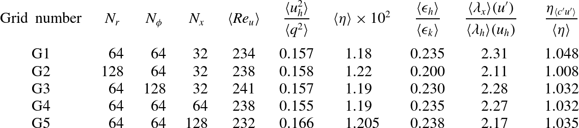
The results reported below were obtained on a cylindrical grid with
 $64\times 64\times 2816$
grid points in the radial, azimuthal and axial directions, respectively. The grid is uniform in the latter two directions and is refined near the wall in the radial direction to capture the strong normal velocity gradients expected within the boundary layer. The performances of this grid resolution are examined in appendix A, especially by considering a somewhat simpler but closely related problem in which the pipe is vertical and the flow is driven by a prescribed axial density gradient whose magnitude is of the same order as that found near
 $x=0$
in the tilted configuration. Results obtained by doubling the radial and azimuthal resolutions only reveal marginal changes on most quantities of interest, especially on the value of
 ${\it\eta}$
. This is in line with the results of § 5 which show that
 ${\it\eta}$
is approximately 0.015 in the core and increases up to 0.018 at the outer edge of the near-wall region: based on these estimates, the above resolution results in a grid spacing,
 ${\it\Delta}$
, smaller than
 $2{\it\eta}$
, a value known to be a good approximation of the size of the smallest eddies (Pope Reference Pope2000, p. 242); it also satisfies the theoretical DNS criterion
 ${\it\Delta}\leqslant {\rm\pi}{\it\eta}$
(Grötzbach Reference Grötzbach1983). To limit computational costs, we adopted a somewhat coarser resolution in the axial direction with
 ${\it\Delta}\approx 4{\it\eta}$
everywhere. As shown in appendix A, doubling or even quadrupling this axial resolution leaves the large-scale variances and the large- and small-scale anisotropies nearly unchanged and modifies
 ${\it\eta}$
by approximately 2 %. The marginal grid dependency observed on
 ${\it\eta}$
and the fact that the energy density near the high-wavenumber cut-off in the velocity (respectively concentration) spectra (not shown) is typically four (respectively three) orders of magnitude lower than in the low-wavenumber range indicate that all energetically significant components of the turbulent field are adequately resolved on the present grid. These various checks provide evidence that the statistics and balances discussed in the rest of the paper are based on robust data.
3. Large-scale characteristics
3.1. Mean fields
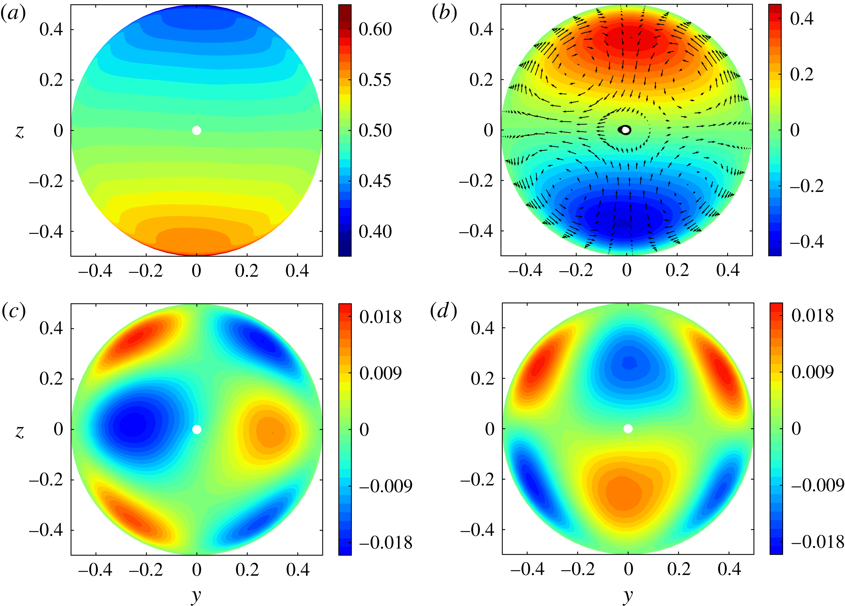
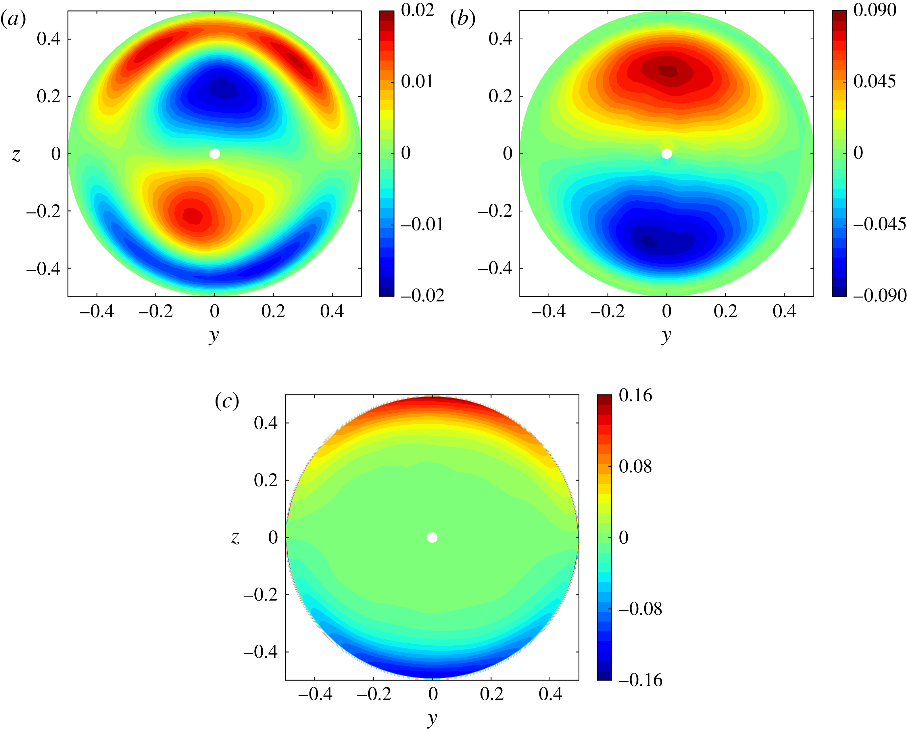
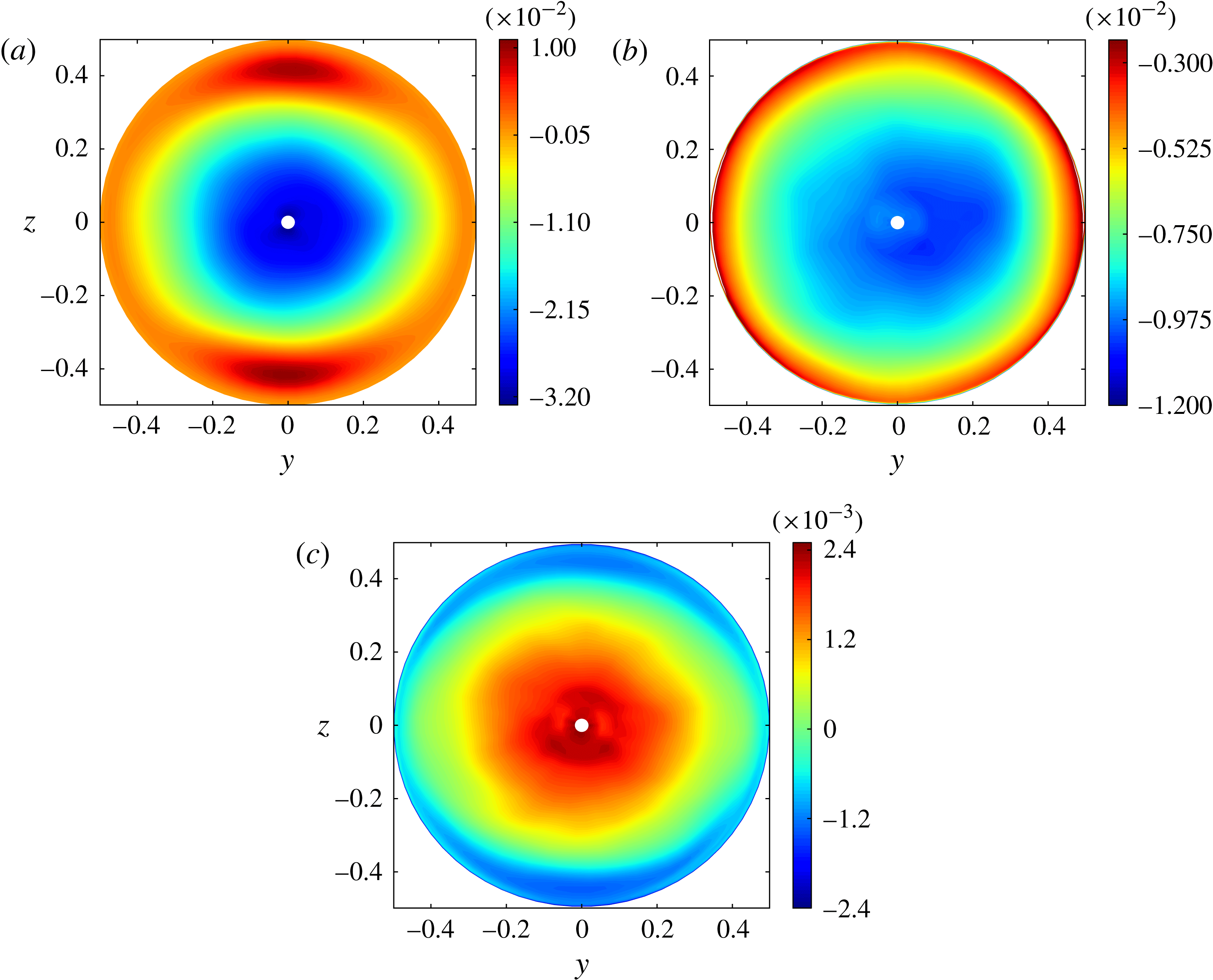
Figure 2(a,b) respectively display the distribution of the mean concentration,
 $\overline{C}$
, and streamwise velocity,
 $\overline{U}$
, in the cross-section
 $x=0$
. Within the core (say
 $|y|\leqslant 0.3,|z|\leqslant 0.35$
), both quantities exhibit a remarkably linear variation with the crosswise coordinate
 $z$
. Nevertheless, the velocity must return to zero at the wall to satisfy the no-slip condition, which results in the presence of an extremum in the
 $\overline{U}$
-profile within each half of any vertical plane, leading to an
 $S$
-shape
 $z$
-variation.
Isocontours of mean concentration and velocity profiles within the pipe cross-section: (a)
 $\overline{C}$
; (b)
 $\overline{U}$
with vectors showing the secondary flow; (c)
 $\overline{V}$
; (d)
 $\overline{W}$
. In all figures, the region corresponding to the small white central disc is excluded because the singularity of the cylindrical coordinate system at
 $y=z=0$
frequently induces inaccuracies in the interpolations (especially the differentiations) involved in the post-processing.

The secondary mean flow discussed by Hallez & Magnaudet (Reference Hallez and Magnaudet2009) is displayed in figure 2(c) and (d). The isovalues indicate that this secondary flow whose maximum intensity is typically 3–5 % that of
 $\overline{U}$
has a four-roll structure which fills entirely the pipe section. As the vectors in Figure 2(b) show, it brings fluid from the axis toward the lateral wall in the
 $z=0$
plane and then from the wall toward the axis within the vertical midplane, thus reducing the crosswise concentration gradient
 $\partial _{z}\overline{C}$
. This transfer of heavy/light fluid towards higher/lower regions of the section is clearly reflected in the curved shape of the near-wall isopycnals in the range
 $|z|\geqslant 0.25$
(see figure 2
a). The mechanism by which the non-zero
 $(\overline{V},\overline{W})$
velocities are generated and sustained (which directly stems from the inhomogeneity of the secondary Reynolds stresses
 $\overline{v^{\prime 2}}-\overline{w^{\prime 2}}$
and
 $\overline{v^{\prime }w^{\prime }}$
), as well as their magnitude (which may be shown to vary as
 $\mathit{Re}_{t}^{-1/2}$
) were analysed in detail in the aforementioned paper to which the reader is referred. In figure 2(c) and (d), it may be noticed that the distributions exhibit significant left–right and top–bottom asymmetries, respectively. At places where these two asymmetries do not compensate exactly, the local divergence of the secondary flow takes non-zero values which are balanced by slow asymmetric
 $X$
-variations of
 $\overline{U}$
to satisfy the incompressibility condition. Obviously, these variations cannot be seen in figure 2(b), owing to the local axial averaging; they could only be discerned by comparing several distributions of
 $\overline{U}$
taken at distinct positions
 $X$
. However, they are responsible for the left–right and top–bottom asymmetries that may be observed in figure 2(b). Although all of these asymmetries would disappear by averaging results at symmetric positions
 $\pm y$
and
 $\pm z$
or by increasing the sampling time, they suggest that the flow exhibits a slow but significant meandering. This will be confirmed in § 5 by examining two-point correlations.
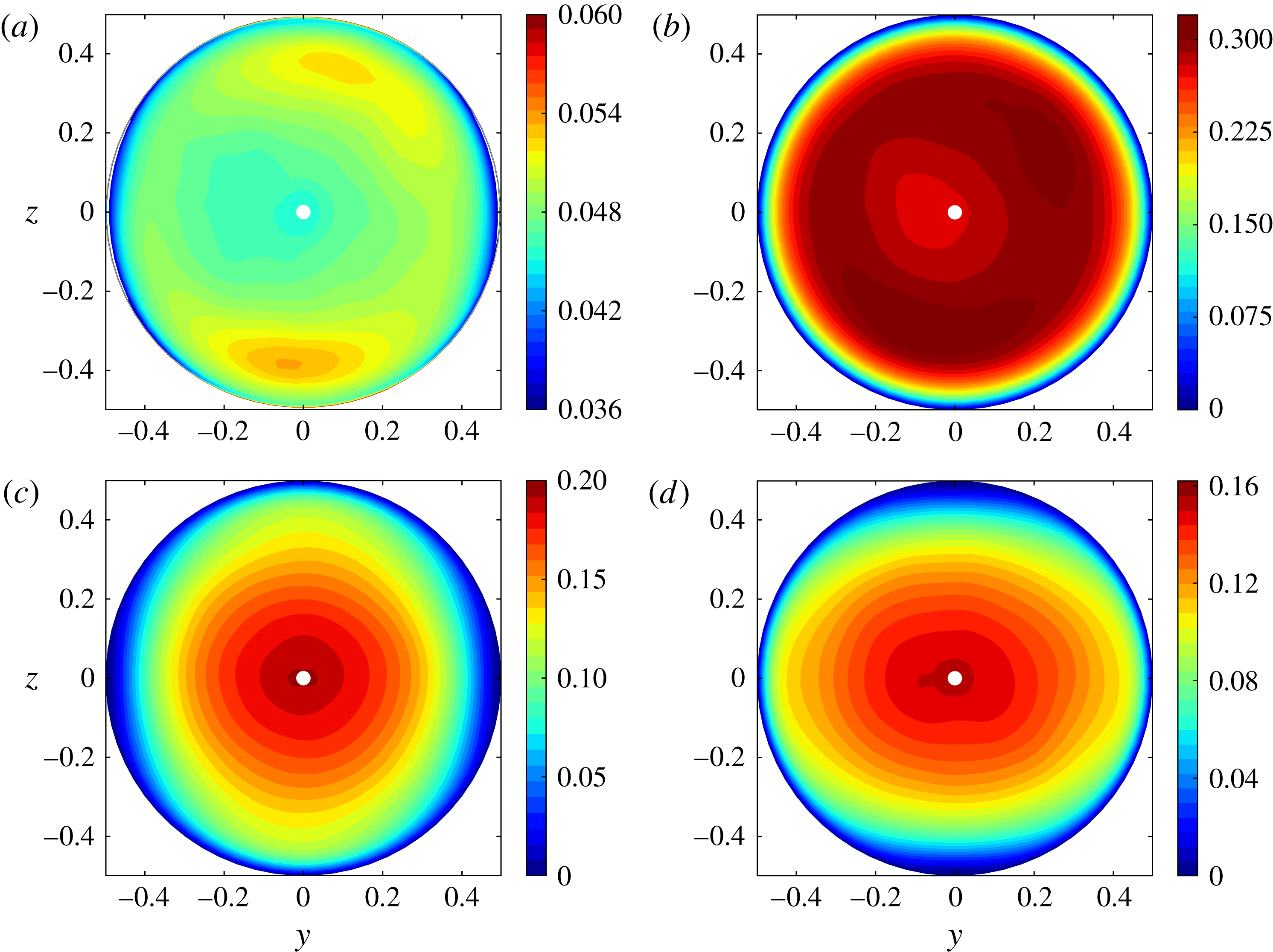
Root mean square values of the velocity and concentration fluctuations within the pipe section: (a)
 $\overline{c^{\prime 2}}^{1/2}$
; (b)
 $\overline{u^{\prime 2}}^{1/2}$
; (c)
 $\overline{v^{\prime 2}}^{1/2}$
; (d)
 $\overline{w^{\prime 2}}^{1/2}$
.

3.2. Turbulent intensities, Reynolds stresses and scalar fluxes
Figure 3 displays the distribution of the root mean square (r.m.s.) values of the concentration fluctuations and those of the three turbulent velocity fluctuations. As figure 3(a) shows, the r.m.s. values of
 $c^{\prime }$
experience little variation (
 $0.047\leqslant \overline{c^{\prime 2}}^{1/2}\leqslant 0.055$
), except in the immediate vicinity of the wall. They reach a broad maximum around the core, along a ring of radius
 $\mathfrak{r}=(y^{2}+z^{2})^{1/2}\approx 0.35$
. The Ellison length scale
 $L_{E}=-\overline{c^{\prime 2}}^{1/2}/\partial _{z}\overline{C}$
can be computed from figures 3(a) and 2(a). This scale may be thought of as the typical distance a fluid particle has to travel along the
 $z$
direction before it either returns towards its equilibrium position or mixes. We find
 $L_{E}\approx 0.34$
, which means that it takes nearly one-third of the pipe diameter for the overturning process to be completed. The distribution of the r.m.s. values of
 $u^{\prime }$
(figure 3
b) is very similar to that of
 $\overline{c^{\prime 2}}^{1/2}$
, except of course close to the wall where it has to return to zero. Again, a broad maximum with
 $\overline{u^{\prime 2}}^{1/2}\approx 0.31$
is observed at the edge of the core, the local minimum on the pipe centreline being approximately 0.275. The spanwise and crosswise fluctuations exhibit a markedly different behaviour. They both reach their maximum on the pipe axis and decrease monotonically toward the periphery. A very similar distribution, with a typical 15 % decrease of the r.m.s. value from the centre to the median radial position
 $\mathfrak{r}=0.25$
as observed here, was reported in the confined RT configuration (with
 $\overline{v^{\prime 2}}=\overline{w^{\prime 2}}$
) by Cholemari & Arakeri (Reference Cholemari and Arakeri2009). Here, as is customary in homogeneous shear (HS) flows (Champagne, Harris & Corrsin Reference Champagne, Harris and Corrsin1970; Tavoularis & Corrsin Reference Tavoularis and Corrsin1981a
; Tavoularis & Karnik Reference Tavoularis and Karnik1989), the crosswise fluctuation is somewhat smaller than the spanwise one (the maximum of
 $\overline{v^{\prime 2}}^{1/2}$
is
 ${\approx}0.19$
whereas that of
 $\overline{w^{\prime 2}}^{1/2}$
is
 ${\approx}0.15$
). In addition, some damping of
 $w^{\prime }$
due to the crosswise stabilizing stratification cannot be ruled out and will indeed be confirmed later. The
 $\overline{v^{\prime 2}}^{1/2}$
distribution exhibits an almost circular symmetry, except near the wall where it has to fall faster to zero along the
 $y$
-axis where
 $v^{\prime }$
is the normal component of the velocity fluctuation than along the
 $z$
-axis where it is a tangential component; the
 $\overline{w^{\prime 2}}^{1/2}$
distribution exhibits a similar near-wall anisotropy with the
 $y$
and
 $z$
directions interchanged. In the core, the isovalues of
 $\overline{w^{\prime 2}}^{1/2}$
appear to be slightly squeezed along the
 $y$
-axis, suggesting some influence of a
 $z$
-dependent mechanism. We shall come back to this point in § 6.3. For future purpose it is appropriate to introduce the Brunt–Väisälä frequency
 $N=(-2\partial _{z}\overline{C}\sin {\it\Theta})^{1/2}$
and define the buoyancy length scale
 $L_{B}=\overline{w^{\prime 2}}^{1/2}/N$
which measures the typical distance a fluid particle could rise in the
 $z$
direction if all of its kinetic energy in that direction were converted into potential energy (Smyth & Moum Reference Smyth and Moum2000). Results from figures 2(a) and 3(d) yield
 $L_{B}\approx 0.58$
, so that the ratio
 $L_{E}/L_{B}$
of the Ellison and buoyancy scales appears to be approximately 0.6.
From (b–d) in figure 3, we may also define an ‘averaged’ r.m.s. turbulent velocity,
 $\mathfrak{u}$
, such that
 $$\begin{eqnarray}\mathfrak{u}=\left(\frac{q^{2}}{3}\right)^{1/2}\quad \text{with}~q^{2}=\mathop{\sum }_{i=1}^{3}\overline{u_{i}^{2}}.\end{eqnarray}$$
The turbulent Reynolds number based on the near-axis values of
 $\mathfrak{u}$
in the region
 $\mathfrak{r}\leqslant 0.1$
is
 $\mathit{Re}_{\mathfrak{u}}=\mathfrak{u}d/{\it\nu}\approx 185$
.
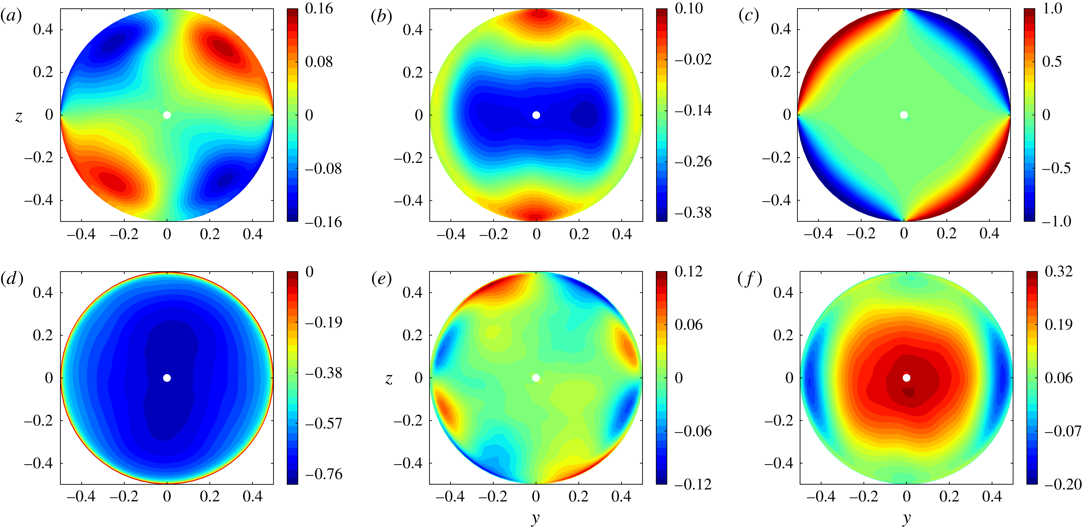
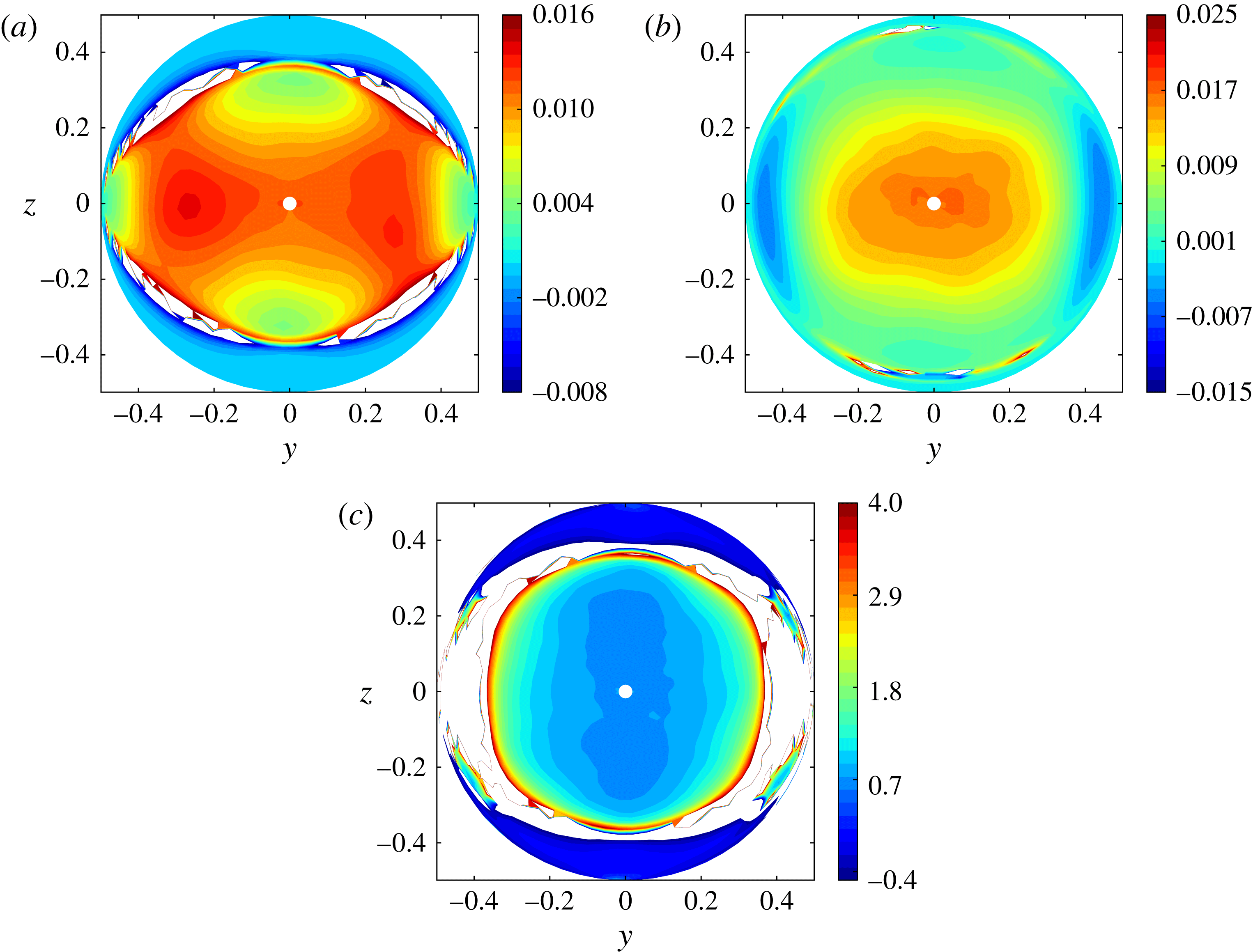
Figure 4(a–c) show the distribution of the three second-order velocity cross-correlation coefficients
 $R_{ij}=\overline{u_{i}u_{j}}/(\overline{u_{i}^{2}}^{1/2}\overline{u_{j}^{2}}^{1/2})~(i\neq j)$
. The
 $R_{13}$
coefficient reaches its maximum in the plane
 $z=0$
and then decreases smoothly as
 $|z|$
increases. It keeps a constant sign essentially everywhere within the section, although small positive values are found very close to the wall around the vertical midplane, typically for
 $|z|\geqslant 0.43$
. Since the isovalues are nearly horizontal in the range
 $|y|\lesssim 0.35$
, it may be concluded that the lateral wall has a marginal influence on
 $\overline{u^{\prime }w^{\prime }}$
in the core. As we saw in figure 2(b), the velocity gradient
 $\partial _{z}\overline{U}$
changes sign around
 $|z|\approx 0.36$
within this central ‘slice’ of the pipe, whereas no such change is observed in figure 3(a). Hence,
 $\overline{u^{\prime }w^{\prime }}$
and
 $\partial _{z}\overline{U}$
have the same sign within the subregion
 $0.36\lesssim |z|\lesssim 0.43$
, i.e. the ‘eddy viscosity’
 $-\overline{u^{\prime }w^{\prime }}/\partial _{z}\overline{U}$
is negative.
For obvious symmetry reasons, second-order cross-correlations involving the spanwise fluctuation
 $v^{\prime }$
must vanish in the
 $y=0$
vertical midplane. They also vanish in the
 $z=0$
midplane since
 $\overline{U}$
and
 $\overline{W}$
are zero there, so that any
 $v^{\prime }$
fluctuation has the same probability to be associated with positive or negative
 $u^{\prime }$
or
 $w^{\prime }$
. Figure 4(a) indicates that
 $R_{12}$
has a four-lobe structure with non-negligible values throughout most of the section. As
 $\partial _{y}\overline{U}$
vanishes for both
 $y=0$
and
 $z=0$
, the extrema of
 $\overline{u^{\prime }v^{\prime }}$
are located along the four diagonals. Along each of them, the extremum is reached near the edge of the core which corresponds to the region where the influence of the wall on the axial velocity is maximum. Note that the maxima of
 $R_{12}$
in the core are smaller than those of
 $R_{13}$
by at least a factor of four, which suggests that they only play a secondary role in the momentum transfer throughout the core. The correlation coefficient
 $R_{23}$
(figure 4
c) also has a four-lobe structure but only exhibits non-negligible values within the peripheral region where the motion of fluid particles is forced to be almost parallel to the wall. This condition yields
 $R_{23}=|1|$
at the wall, as confirmed by figure 4(c). It also dictates the sign of
 $\overline{v^{\prime }w^{\prime }}$
: for instance, in the first quadrant, fluid particles moving up faster than the secondary flow have a positive
 $w^{\prime }$
but their spanwise velocity is negative on average and exceeds
 $\overline{V}$
, so that they have a negative
 $v^{\prime }$
, resulting eventually in the negative sign of
 $\overline{v^{\prime }w^{\prime }}$
. The correlation
 $\overline{v^{\prime }w^{\prime }}$
is actually directly involved in the generation of the mean secondary flow, as discussed by Hallez & Magnaudet (Reference Hallez and Magnaudet2009).
Cross-correlations coefficients
 $R_{ij}=\overline{u_{i}u_{j}}/(\overline{u_{i}^{2}}^{1/2}\overline{u_{j}^{2}}^{1/2})~(i\neq j)$
and normalized fluxes
 $F_{i}=\overline{c^{\prime }u_{i}}/(\overline{c^{\prime 2}}^{1/2}\overline{u_{i}^{2}}^{1/2})$
within the pipe section: (a)
 $R_{12}$
; (b)
 $R_{13}$
; (c)
 $R_{23}$
; (d)
 $F_{1}$
; (e)
 $F_{2}$
; (f)
 $F_{3}$
.

Figure 4(d–f) display the three components of the normalized turbulent fluxes
 $F_{i}=\overline{c^{\prime }u_{i}}/(\overline{c^{\prime 2}}^{1/2}\overline{u_{i}^{2}}^{1/2})$
. Their maxima are found to be very dissimilar:
 $F_{1}$
is larger by a factor of 2.5 than
 $F_{3}$
which itself is typically three times larger than
 $F_{2}$
. Figure 4(d) reveals that the axial component experiences little variation throughout the cross-section, except of course in the peripheral region where it goes to zero at the wall. Therefore its behaviour resembles very much that of
 $\overline{u^{\prime 2}}$
, underlining the direct link between density and axial velocity fluctuations. Figure 4(e) indicates that
 $F_{2}$
is negligibly small throughout the core, in line with the negligibly small spanwise gradient
 $\partial _{y}\overline{C}$
. Although quite ‘noisy’ because of the low magnitude of the extrema and hence its poorly converged geometry, an eight-lobe structure can be identified at the pipe periphery, with positive and negative values alternating within each quadrant. In the part of each quadrant closest to the vertical midplane, where the largest values are found and the lobes are ‘stuck’ to the wall, the spanwise gradient
 $\partial _{y}\overline{C}$
is large (typically of the same order as
 $\partial _{z}\overline{C}$
according to figure 2
a) and may thus be expected to drive the generation of
 $\overline{c^{\prime }v^{\prime }}$
. Close to the midplane
 $z=0$
, where the lobes are distinctly detached from the wall, this gradient is much smaller, suggesting that the generation of
 $\overline{c^{\prime }v^{\prime }}$
is controlled by other mechanisms such as the spanwise transport of
 $c^{\prime }v^{\prime }$
by
 $v^{\prime }$
itself. Figure 4(f) shows that the distribution of
 $F_{3}$
is quite similar to that of
 $R_{13}$
: it reaches its maximum on the axis an then decreases monotonically towards the wall, keeping a constant sign all along except close to the plane
 $z=0$
where significant negative values are found near the wall. Since
 $\partial _{z}\overline{C}$
is positive everywhere, these negative values correspond to counter-gradient fluxes; their origin will be elucidated in § 6.3.
Disregarding cross-correlations involving
 $v^{\prime }$
(because their distribution is clearly connected to the wall influence), the observed behaviours may be divided into two families. On the one hand
 $\overline{c^{\prime 2}}$
,
 $\overline{u^{\prime 2}}$
and
 $\overline{c^{\prime }u^{\prime }}$
exhibit little variation within the core, with a broad maximum around it. On the other hand,
 $\overline{v^{\prime 2}}$
,
 $\overline{w^{\prime 2}}$
,
 $\overline{u^{\prime }w^{\prime }}$
and
 $\overline{c^{\prime }w^{\prime }}$
reach their maximum on the axis and decrease monotonically toward the wall. As we shall see later, this radial decrease has several distinct origins, depending on which component is considered.
4. Mean concentration and momentum balances
The mean concentration (i.e. density) and axial momentum balances are established and discussed in appendix B. This discussion shows that, at leading order in the pipe aspect ratio
 ${\it\epsilon}$
, all terms involving derivatives with respect to the axial direction are negligible in the latter. The situation is different for the
 $\overline{C}$
balance where the forcing term
 ${\it\epsilon}\overline{U}\partial _{X}\langle C\rangle$
corresponding to the axial transport of the density gradient is found to play a key role.
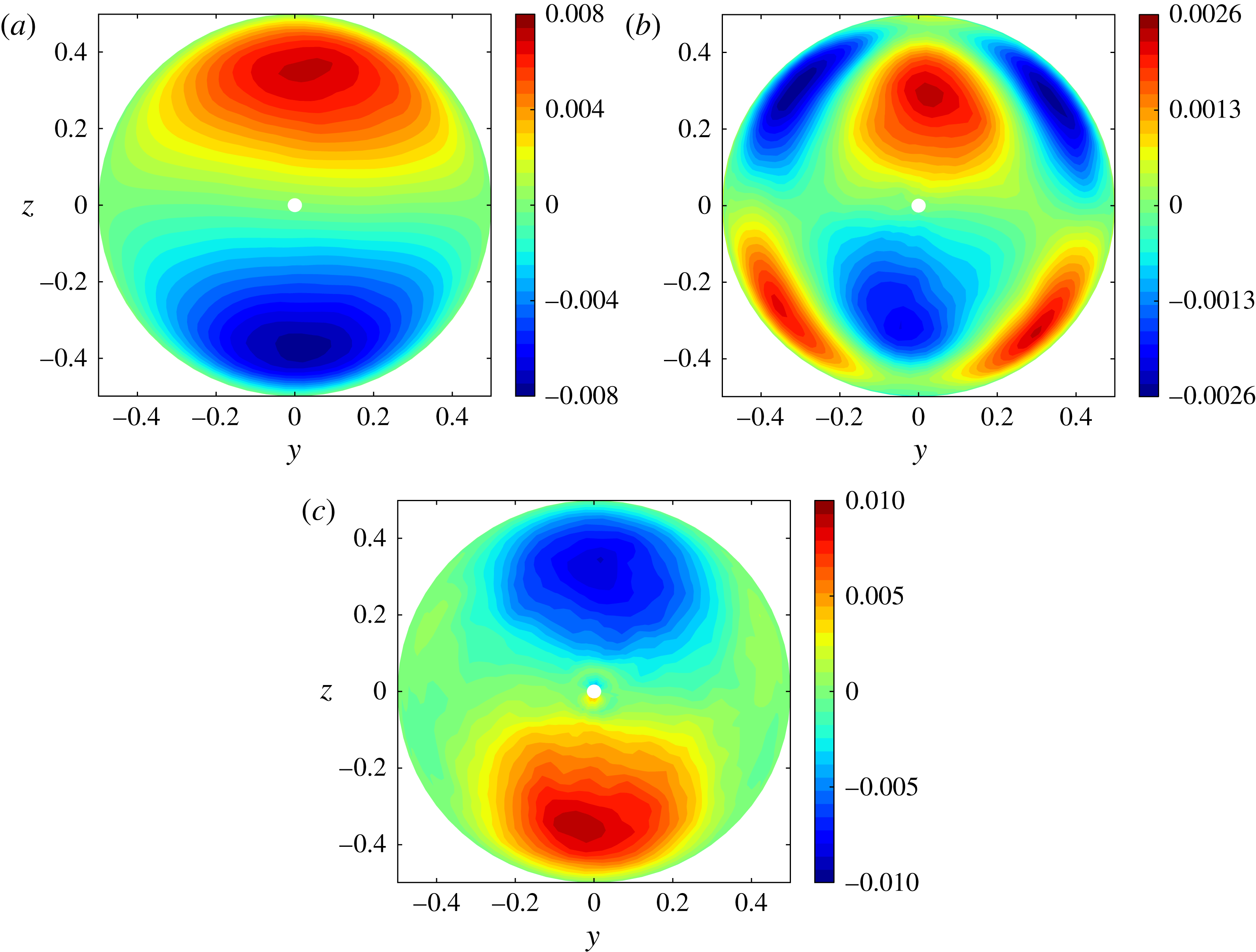
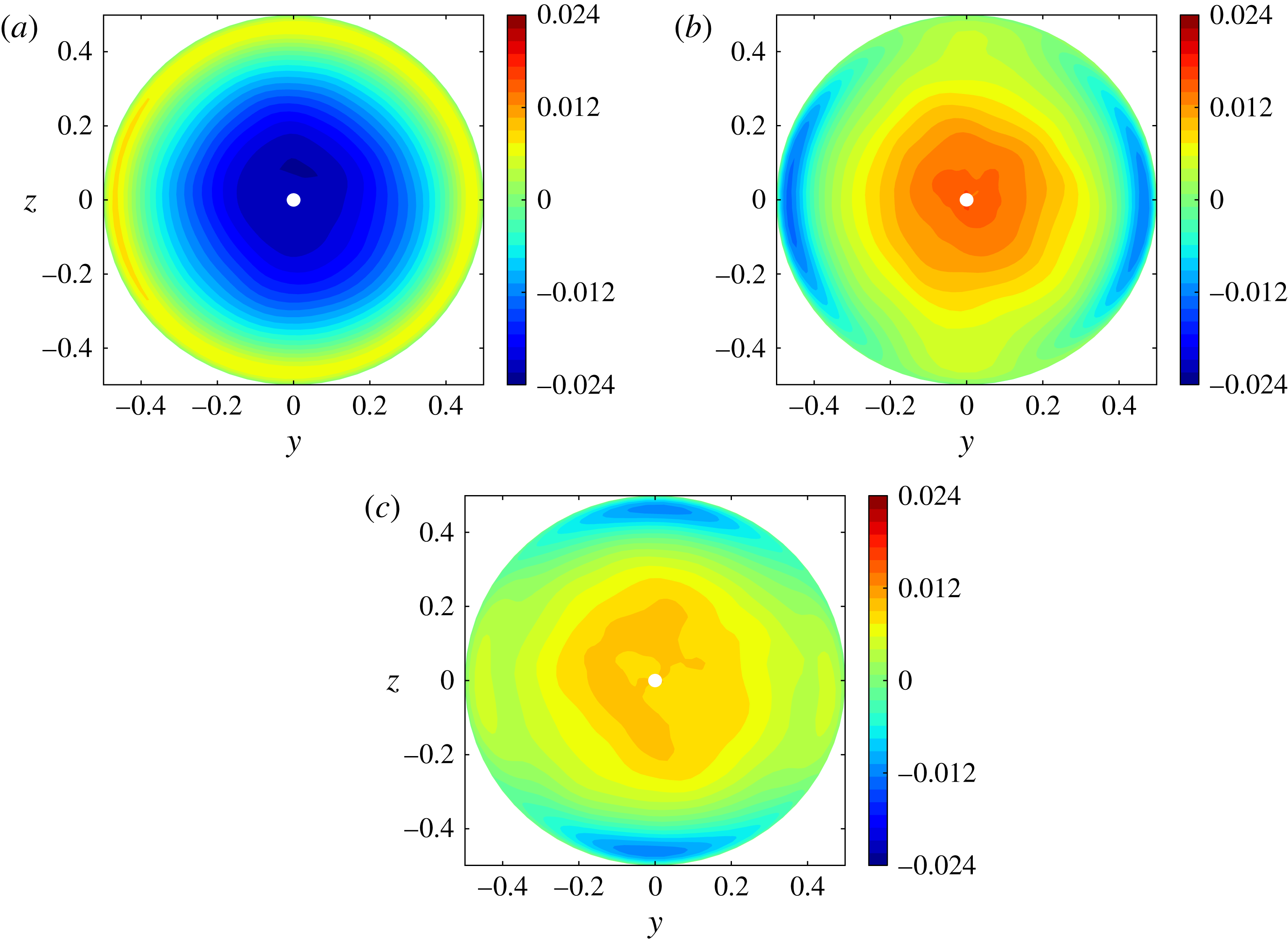
Contributions to the axial mean momentum balance within the cross-sectional plane: (a) transport by the secondary flow; (b) contribution of Reynolds stresses; (c) viscous diffusion.

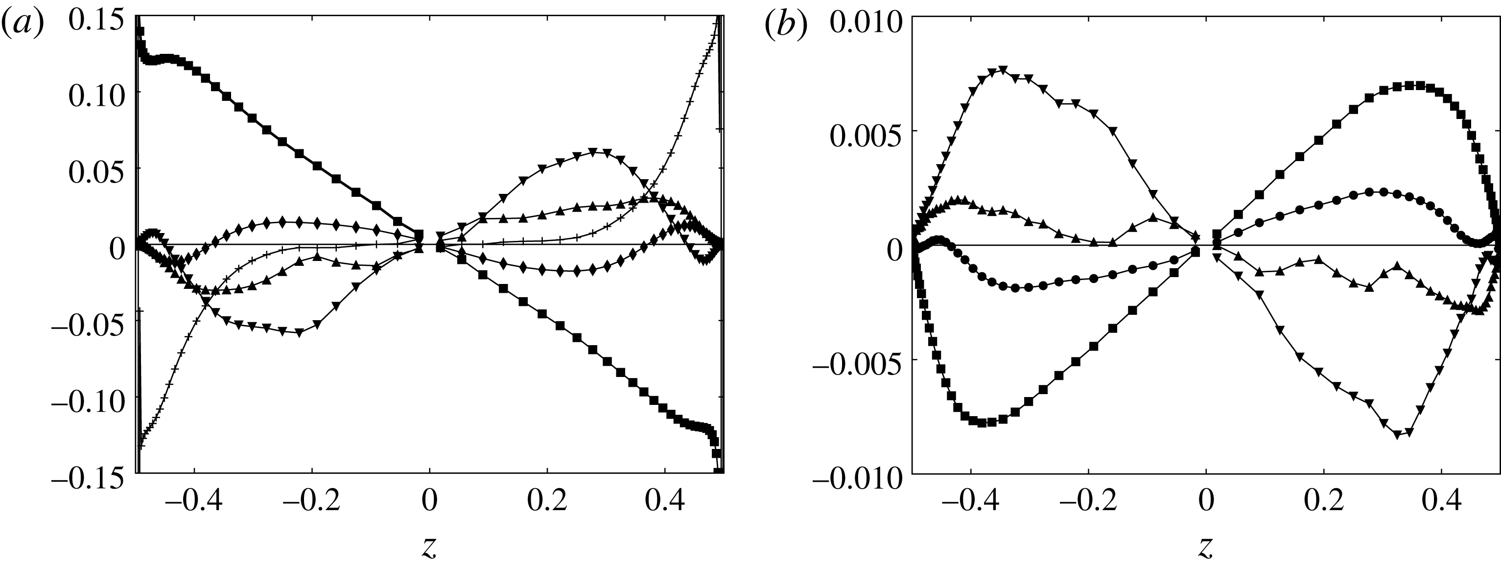
Mean budgets in the vertical diametrical plane. (a) Axial momentum budget (▪,
 $2\cos {\it\Theta}{\rm\Delta}C$
; ♦,
 $\overline{W}\partial _{z}\overline{U}$
; ▴,
 $\partial _{y}\overline{u^{\prime }v^{\prime }}$
; ▾,
 $\partial _{z}\overline{u^{\prime }w^{\prime }}$
;
+,
 $-\mathit{Re}_{t}^{-1}{\rm\nabla}_{\bot }^{2}\overline{U}$
). (b) Concentration budget (▪,
 ${\it\epsilon}\overline{U}\partial _{X}\overline{C}$
; ●,
 $\overline{W}\partial _{z}\overline{C}$
; ▴,
 $\partial _{y}\overline{c^{\prime }v^{\prime }}$
; ▾,
 $\partial _{z}\overline{c^{\prime }w^{\prime }}$
).

4.1. Streamwise momentum balance
According to appendix B, the mean momentum balance in the axial direction reads at leading order
 $$\begin{eqnarray}2\cos {\it\Theta}{\rm\Delta}C+\overline{V}\partial _{y}\overline{U}+\overline{W}\partial _{z}\overline{U}+\partial _{y}\overline{u^{\prime }v^{\prime }}+\partial _{z}\overline{u^{\prime }w^{\prime }}-\mathit{Re}_{t}^{-1}{\rm\nabla}_{\bot }^{2}\overline{U}\approx 0,\end{eqnarray}$$
where
 $\boldsymbol{{\rm\nabla}}_{\bot }$
denotes the two-dimensional gradient in the cross-sectional plane and
 ${\rm\Delta}C(X,y,z,T)=\overline{C}(X,y,z,T)-\langle C\rangle (X,T)$
its the local transverse stratification. The first contribution,
 $2\cos {\it\Theta}{\rm\Delta}C$
, represents a forcing resulting from the combined action of the axial gravity component and the stabilizing stratification within the cross-sectional plane. The spatial distribution of this contribution is similar to that displayed in figure 2(a) with a uniform shift of 0.5. Figure 5 shows the distribution of the other three groups of terms involved in (4.1) while figure 6(a) shows the profile of all significant terms in the vertical diametrical plane
 $y=0$
. As figure 5(c) reveals, the contribution of viscous effects is significant only near the wall, in the top and bottom parts of the section. The secondary flow provides a small, albeit significant, contribution in two distinct regions. First it tends to lower the magnitude of
 $|\overline{U}|$
near the wall by bringing low-velocity fluid toward the high-velocity region located around the plane
 $y=0$
. Then it tends to counteract the mean shear
 $\partial _{z}\overline{U}$
by bringing fluid from the high-
 $|\overline{U}|$
region located around
 $y=0,~|z|\approx 0.35$
toward the low-momentum region located around the pipe axis. Finally, the momentum flux associated with the Reynolds stresses (figure 5
b) provides the contribution that balances most of the forcing term in the core, thus tending to homogenize the flow field. Its distribution is similar to that of the axial velocity, with its two extrema located close to those of
 $\overline{U}$
, albeit somewhat closer to the axis (compare figures 5
b and 2
b). As figure 6(a) indicates, the contribution of the spanwise Reynolds stress
 $\overline{u^{\prime }v^{\prime }}$
is far from negligible since it represents approximately 40 % that of
 $\overline{u^{\prime }w^{\prime }}$
in the core.
Apart from the role of the secondary flow and spanwise Reynolds stress (which nearly balance each other in the central region, as shown by figure 6
a), the present axial momentum balance is qualitatively similar to that encountered in the buoyancy-driven flow in a vertical channel with differentially heated walls (VCDHW). In particular, the linear stratification in the
 $z$
direction is responsible for the quadratic variation of the main shear stress
 $\overline{u^{\prime }w^{\prime }}$
in both cases.
4.2. Mean concentration balance
According to the analysis of appendix B, the mean concentration balance reads at leading order in
 ${\it\epsilon}$
 $$\begin{eqnarray}{\it\epsilon}\overline{U}\partial _{X}\langle C\rangle +\overline{V}\partial _{y}\overline{C}+\overline{W}\partial _{z}\overline{C}+\partial _{y}\overline{v^{\prime }c^{\prime }}+\partial _{z}\overline{w^{\prime }c^{\prime }}\approx 0.\end{eqnarray}$$
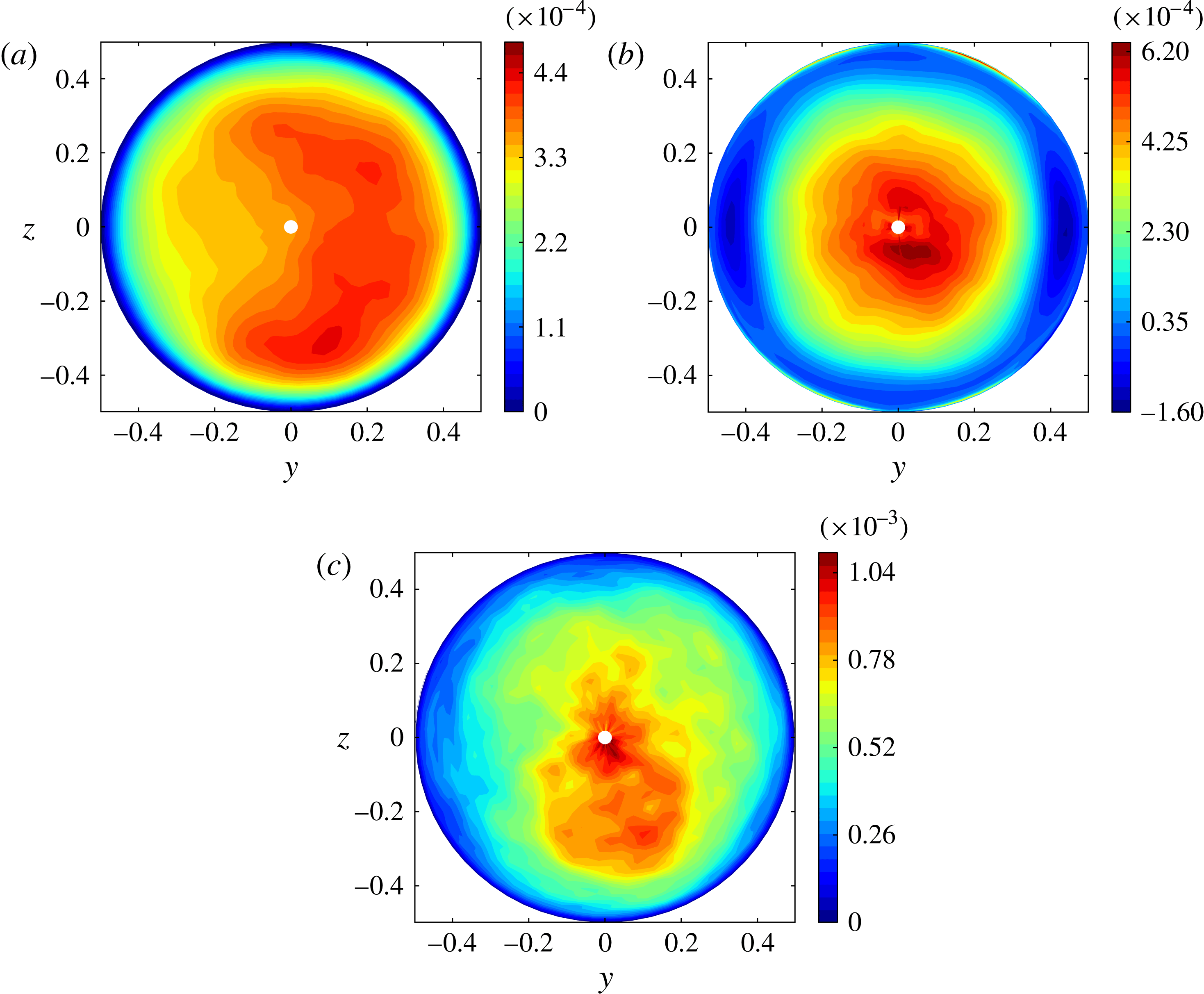
Figure 7 shows the distribution of the three groups of terms involved in (4.2); the profile of the various terms along the vertical diametrical plane is shown in figure 6(b). Both figures display the distribution of
 ${\it\epsilon}\overline{U}\partial _{X}\overline{C}$
rather than that of
 ${\it\epsilon}\overline{U}\partial _{X}\langle C\rangle$
. However, the striking similarity between figure 7(a) and the distribution of
 $\overline{U}$
shown in figure 2(b) proves that
 $\partial _{X}\overline{C}$
is essentially constant throughout the cross-section. This confirms that the
 $X$
-derivative of
 ${\rm\Delta}C$
is negligibly small, implying
 $\partial _{X}\overline{C}\approx \partial _{X}\langle C\rangle$
, as concluded in appendix B. In other words, the source that drives the variations of the turbulent fluxes
 $\overline{c^{\prime }v^{\prime }}$
and
 $\overline{c^{\prime }w^{\prime }}$
across the section (and hence indirectly those of
 $\overline{C}$
) is the non-uniform transport of the small axial mean concentration gradient
 ${\it\epsilon}\partial _{X}\langle C\rangle$
by the axial mean flow
 $\overline{U}$
. Although 3–4 times smaller, the contribution of the secondary flow to the transport of
 $\overline{C}$
is significant. As shown in figure 7(b), it tends to homogenize the fluid within the section by bringing light (respectively heavy) fluid from the top (respectively bottom) to the centre along the
 $z$
-axis, and heavy (respectively light) fluid to the top (respectively bottom) along the wall. Finally, the turbulent fluxes bring fluid from the well-mixed near-axis region where
 $\overline{C}\approx \langle C\rangle$
toward the high- and low-concentration regions near the top and bottom. This is why the spatial distribution of their two-dimensional divergence (figure 7
c) is close to that of the axial velocity, especially in the central ‘slice’
 $|y|\leqslant 0.25$
. Again, the contribution of the spanwise flux
 $\overline{c^{\prime }v^{\prime }}$
is significant, being typically one-quarter that of
 $\overline{c^{\prime }w^{\prime }}$
in the core.
Contributions to the mean concentration balance in the cross-sectional plane: (a) axial transport; (b) transport by the secondary flow; (c) turbulent transport.

Note that the present quadratic variation of
 $\overline{c^{\prime }w^{\prime }}$
contrasts with the flat profile of the turbulent heat flux observed in the core of pressure-driven channel or pipe flows or VCDHW flows with isothermal walls. The reason is of course that the source term
 ${\it\epsilon}\overline{U}\partial _{X}\overline{C}$
has no counterpart in those cases, forcing the total crosswise heat flux to be
 $z$
-independent.
5. Length scales and dissipation
5.1. Two-point autocorrelations and integral scales
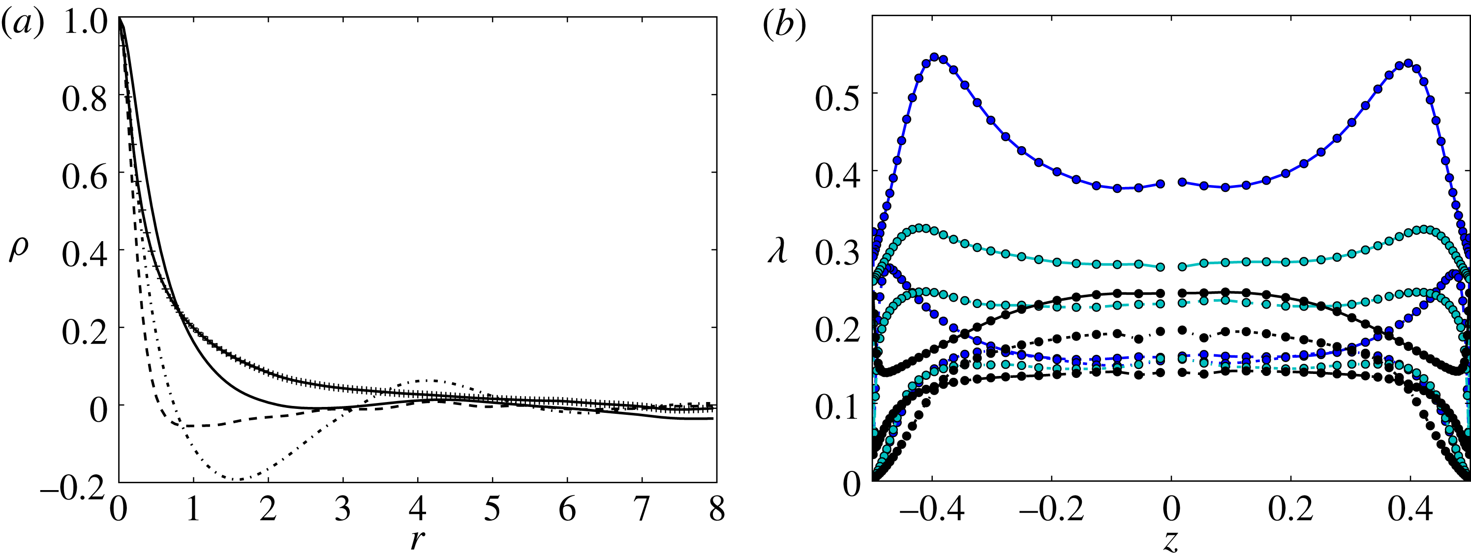
Figure 8(a) shows the typical behaviour of the longitudinal two-point velocity correlations,
 ${\it\rho}_{ii}(r)$
, in the core within the central vertical strip
 $|y|\lesssim 0.175$
. In particular, it reveals that the spanwise movements remain significantly correlated over distances up to
 $r\approx 5$
whereas the axial and crosswise movements are virtually uncorrelated beyond
 $r=2$
. Unlike
 ${\it\rho}_{11}$
and
 ${\it\rho}_{33}$
,
 ${\it\rho}_{22}$
exhibits strong oscillations with a marked minimum and a secondary maximum at
 $r\approx 1.6$
and
 $r\approx 4.2$
, respectively. These features indicate a slow meandering of the flow in the spanwise direction, in line with the significant left–right asymmetry observed in the
 $\overline{V}$
-distribution in figure 2. The above two-point correlations were used to compute the integral length scales,
 $L_{ii}^{x}$
, through two distinct definitions, namely the integral of the correlation up to its first zero (all correlations exhibit negative values within some range of
 $r$
), and the specific value of
 $r$
at which the correlation reaches this first zero. We find
 $L_{22}^{x}/L_{33}^{x}$
to be approximately 1.35 with both definitions, while the ratio
 $L_{11}^{x}/L_{33}^{x}$
is in the range 2.6–3.9, depending on which definition is considered (the two ratios would respectively be 1.0 and 2.0 in HIT, respectively).
Two-point correlations and Taylor microscales. (a) Longitudinal two-point correlations resulting from an average taken over two symmetric arcs of a circle whose middles are located on the
 $z$
-axis at
 $z=\pm 0.25$
and whose length covers a 90° angle in the azimuthal direction (corresponding to 16 grid points): solid line,
 ${\it\rho}_{11}$
; dash-dotted line,
 ${\it\rho}_{22}$
; dashed line,
 ${\it\rho}_{33}$
; solid line with crosses,
 ${\it\rho}_{cc}$
. (b) Profiles of the Taylor microscales along the
 $z$
-axis. From top to bottom in the core, the solid lines refer to
 ${\it\lambda}_{x}(u^{\prime }),{\it\lambda}_{x}(v^{\prime }),{\it\lambda}_{x}(w^{\prime })$
, the dashed lines to
 ${\it\lambda}_{y}(v^{\prime }),{\it\lambda}_{y}(u^{\prime }),{\it\lambda}_{y}(w^{\prime })$
and the dash-dotted lines to
 ${\it\lambda}_{z}(w^{\prime }),{\it\lambda}_{z}(u^{\prime }),{\it\lambda}_{z}(v^{\prime })$
, respectively.

Figure 8(a) also displays the longitudinal two-point scalar correlation,
 ${\it\rho}_{cc}(r)$
. It is immediately seen that it keeps significant positive values over larger distances than any velocity fluctuation. This results in large values of the corresponding axial integral scale: using the definition based on the position of the first zero, we find
 $L_{cc}^{x}\approx 6.75$
(to be compared with
 $L_{11}^{x}\approx 2.19$
), an indication that the large-scale density field contains long plumes travelling along the pipe, in line with the findings of Cholemari & Arakeri (Reference Cholemari and Arakeri2009), Gibert et al. (Reference Gibert, Pabiou, Tisserand, Gertjerenken, Castaing and Chillà2009) and Tisserand et al. (Reference Tisserand, Creyssels, Gibert, Castaing and Chillà2010) in vertical pipe and channel configurations.
5.2. Taylor microscales and mechanical dissipation
Figure 8(b) displays the profiles along the
 $z$
-axis of all nine Taylor microscales,
 ${\it\lambda}_{j}(u_{i})$
, computed using the classical definition
 $$\begin{eqnarray}{\it\lambda}_{j}^{2}(u_{i})=\frac{2\overline{u_{i}^{2}}}{\overline{(\partial u_{i}/\partial x_{j})^{2}}},\end{eqnarray}$$
(no summation on
 $i$
). Note that computing the
 $y$
- and
 $z$
-derivatives of Cartesian velocity components from data obtained on a cylindrical grid requires geometrical transformations that induce some inaccuracy near the singular axis
 $y=z=0$
, leading to the oscillations (respectively colour blobs) visible in the central part of on some curves (respectively maps). Two major features emerge from figure 8(b). One is the large anisotropy of the small-scale flow, with in particular streamwise length scales
 ${\it\lambda}_{x}(u_{i})$
significantly larger than their spanwise and crosswise counterparts for all three velocity components (as shown in appendix A, this is by no means an artifact related to the coarser resolution employed in the axial direction). The second is the weak influence of the wall in the central half of the section: except for
 ${\it\lambda}_{x}(u^{\prime })$
which exhibits a 15 % increase from the axis to
 $|z|=0.25$
and to some extent
 ${\it\lambda}_{x}(w^{\prime })$
which decreases by roughly 10 % over the same distance, all other
 ${\it\lambda}_{j}(u_{i})$
vary only by a few per cent within this range. This indicates that the small-scale structure is nearly unaffected by confinement effects within the core. Examining in more detail the isotropy/anisotropy properties revealed by figure 8(b), it may first be observed that
 ${\it\lambda}_{y}(u^{\prime })\approx {\it\lambda}_{y}(w^{\prime })\approx {\it\lambda}_{z}(u^{\prime })\approx {\it\lambda}_{z}(v^{\prime })$
and that the latter four length scales are nearly equal to
 ${\approx}({\it\lambda}_{y}(v^{\prime }))/\sqrt{2}$
as would be expected for isotropic turbulence. Therefore, some kind of small-scale isotropy is preserved within the section, the only exception being
 ${\it\lambda}_{z}(w^{\prime })$
which is only approximately 80 % of
 ${\it\lambda}_{y}(v^{\prime })$
whereas the two should be equal, were the isotropy in the
 $(y,z)$
plane strictly satisfied. In contrast all three axial length scales are much larger than those in the
 $y$
or
 $z$
directions. In particular
 ${\it\lambda}_{x}(v^{\prime })$
is twice as large as
 ${\it\lambda}_{z}(v^{\prime })$
and
 ${\it\lambda}_{x}(u^{\prime })$
is also twice as large as
 ${\it\lambda}_{z}(w^{\prime })$
. Therefore, it may qualitatively be concluded that most of the fluctuating vorticity is concentrated within structures whose axial length is on average twice as large as their transverse size.
Results of figures 8(b) and 3 may be combined to compute the mechanical dissipation rate per unit mass which writes
 $$\begin{eqnarray}{\it\epsilon}_{k}=\mathop{\sum }_{i=1}^{3}{\it\epsilon}_{i}=\mathit{Re}_{t}^{-1}\mathop{\sum }_{i=1}^{3}\left\{\overline{u_{i}^{2}}\mathop{\sum }_{j=1}^{3}\frac{1}{{\it\lambda}_{j}^{2}(u_{i})}\right\},\end{eqnarray}$$
where
 ${\it\epsilon}_{i}$
denotes the diagonal component of the dissipation tensor along direction
 $i$
.
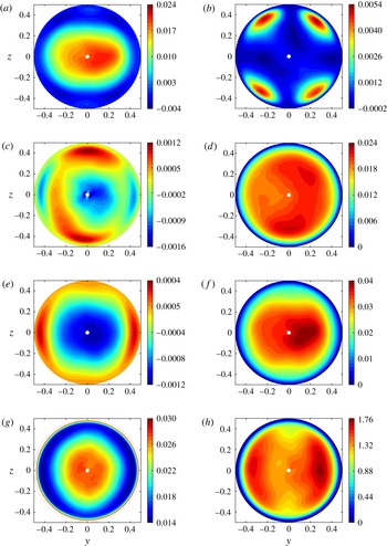
As shown in figure 9(g),
 ${\it\epsilon}_{k}$
exhibits a nearly flat profile in the core with a value close to 0.0275. Then it gently decreases down to a minimum approximately 0.014 reached near the outer edge of the near-wall region. Finally, it sharply increases and peaks at the wall where
 ${\it\epsilon}_{k}\approx 0.068$
. Although they all reveal qualitatively similar radial variations, a strong anisotropy exists among the three diagonal components
 ${\it\epsilon}_{i}$
(not shown),
 ${\it\epsilon}_{1}$
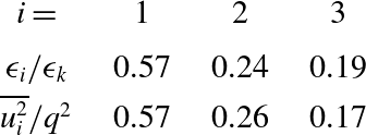
being typically three times larger than the other two in the core. This anisotropy may be compared with that existing among the components of the r.m.s. velocity fluctuations. As shown in table 1, the ratio
 ${\it\epsilon}_{i}/{\it\epsilon}_{k}$
closely follows the ratio
 $\overline{u_{i}^{2}}/q^{2}$
, giving support to Rotta’s model
 ${\it\epsilon}_{i}/{\it\epsilon}_{k}=\overline{u_{i}^{2}}/q^{2}$
(Rotta Reference Rotta1951). Hence, the anisotropy of the large-scale field turns out to have a direct footprint on the small-scale motion. This may be interpreted as a low-Reynolds-number effect, but similar levels of small-scale anisotropy have been reported in uniform shear flows with higher Reynolds numbers (Tavoularis & Corrsin Reference Tavoularis and Corrsin1981b
; Pumir & Schraiman Reference Pumir and Schraiman1995). Thus present data may also be seen as suggesting that the small-scale phenomenology is deeply influenced by the mean shear. Extra runs at higher Reynolds number would be necessary to disentangle the two possibilities.
Contributions to the production/destruction of the turbulent energy within the pipe section: (a)
 $P_{\overline{U}_{z}}$
; (b)
 $P_{\overline{U}_{y}}$
; (c)
 $P_{sec}$
; (d)
 $P_{F_{1}}$
; (e)
 $P_{F_{3}}$
; (f) TKE production,
 $P_{k}=P_{\overline{U}_{z}}+P_{\overline{U}_{y}}+P_{sec}+P_{F_{1}}+P_{F_{3}}$
; (g) dissipation rate
 ${\it\epsilon}_{k}$
(for
 $\mathfrak{r}\geqslant 0.47$
, the near-wall values of
 ${\it\epsilon}_{k}$
are out of scale, the peak value at the wall being 0.068); (h) ratio
 $P_{k}/{\it\epsilon}_{k}$
of TKE production over dissipation.

Comparison between the normalized diagonal components of the mechanical dissipation and those of the normalized variance of the fluctuating velocity (values are taken in the central region
 $\mathfrak{r}\leqslant 0.15$
).

Combining (5.2) with the definition (3.1), we may generalize the classical HIT relationship
 ${\it\epsilon}_{k}=15\mathit{Re}_{t}^{-1}\mathfrak{u}^{2}/{\it\lambda}^{2}$
. Then, defining an ‘averaged’ Taylor microscale,
 ${\it\lambda}$
, as
 ${\it\lambda}=\mathit{Re}_{t}^{-1/2}\mathfrak{u}\sqrt{15/{\it\epsilon}_{k}}$
, we find
 ${\it\lambda}\approx 0.165$
and
 $$\begin{eqnarray}\mathit{Re}_{{\it\lambda}}=\mathit{Re}_{t}{\it\lambda}\mathfrak{u}=\mathit{Re}_{t}^{1/2}\sqrt{\frac{5}{3{\it\epsilon}_{k}}}q^{2}\approx 31.\end{eqnarray}$$
With
 ${\it\epsilon}_{k}$
at hand, we can compute the three characteristic length scales that allow the range of scales affected by viscosity, stabilizing stratification or shear to be estimated in the framework of Kolmogorov theory. First, the Kolmogorov scale,
 ${\it\eta}=\mathit{Re}_{t}^{-3/4}{\it\epsilon}_{k}^{-1/4}$
, is found to be
 ${\it\eta}\approx 1.5\times 10^{-2}\approx 0.09{\it\lambda}$
. The Ozmidov scale,
 $L_{O}=({\it\epsilon}_{k}/N^{3})^{1/2}$
, and the Corrsin scale,
 $L_{C}=\{{\it\epsilon}_{k}/(\partial _{z}\overline{U})^{3}\}^{1/2}$
, are indicators of the scale beyond which stabilizing stratification and shear effects affect the local flow structure, respectively. Present data indicate
 $L_{O}\approx 1.30$
and
 $L_{C}\approx 0.12$
. These estimates suggest that stratification barely affects the local flow structure at any scale, while the mean shear has a much stronger influence which extends down to structures with a size of a few
 ${\it\eta}$
. However, it must be kept in mind that the above definitions implicitly assume turbulence to be isotropic, which is far from being the case here. In particular, as shown in table 1,
 ${\it\epsilon}_{3}$
is only approximately 20 % of
 ${\it\epsilon}_{k}$
, so that
 $L_{O3}=({\it\epsilon}_{3}/N^{3})^{1/2}$
should be a more relevant scale to characterize the possible influence of stabilizing stratification on
 $w^{\prime }$
. With this definition one finds
 $L_{O3}\approx 0.54$
, which now suggests that stratification has some effect on the large-scale structure of
 $w^{\prime }$
, although it certainly has a nearly negligible influence on
 $u^{\prime }$
. Section 6 will confirm this conjecture.
6. Energetics of the turbulent field
6.1. The
 $\overline{u_{i}^{2}}$
and
$q^{2}$
balances


Results discussed in the previous sections indicate that the turbulent field is strongly anisotropic at all scales and reveal a significant radial inhomogeneity of the diagonal Reynolds stresses
 $\overline{u_{i}^{2}}$
. To get further insight into the mechanisms that generate and sustain these characteristics, it is necessary to examine the main contributions to the three
 $\overline{u_{i}^{2}}$
budgets. Numerical data indicate that the time rate-of-change term
 ${\it\epsilon}\partial _{T}\overline{u_{i}^{2}}$
and all contributions involving derivatives in the axial direction are negligibly small everywhere. Transport by the secondary flow and viscous diffusion are also found to be very small throughout the core and are significant only in the near-wall region, especially regarding the latter which has to balance
 ${\it\epsilon}_{i}$
at the wall. Hence, the
 $\overline{u_{i}^{2}}$
balance in the core essentially reduces to
 $$\begin{eqnarray}P_{i}+{\it\Phi}_{i}-{\it\epsilon}_{i}-\boldsymbol{{\rm\nabla}}_{\bot }\boldsymbol{\cdot }\boldsymbol{J}_{i}\approx 0,\end{eqnarray}$$
where
 $P_{i}$
is the ‘production’ term responsible for the conversion of the mean flow kinetic energy or the potential energy into
 $\overline{u_{i}^{2}}$
,
 ${\it\Phi}_{i}=\overline{p^{\prime }\partial _{i}u_{i}}$
(no summation on
 $i$
) is the pressure–strain correlation responsible for energy redistribution between the three components of the fluctuating motion, and the contribution of
 $\boldsymbol{J}_{i}=1/2\overline{u_{i}^{2}\boldsymbol{v}_{\bot }}+\overline{p^{\prime }v^{\prime }}\boldsymbol{e}_{\boldsymbol{y}}{\it\delta}_{i2}+\overline{p^{\prime }w^{\prime }}\boldsymbol{e}_{\boldsymbol{z}}{\it\delta}_{i3}$
is the lateral flux corresponding to the in-plane transport of
 $\overline{u_{i}^{2}}$
by turbulent fluctuations,
 $p^{\prime }$
being the pressure fluctuation and
 $\boldsymbol{v}_{\bot }=v^{\prime }\boldsymbol{e}_{\boldsymbol{y}}+w^{\prime }\boldsymbol{e}_{\boldsymbol{z}}$
the velocity fluctuation within the cross-sectional plane (
 $\boldsymbol{e}_{\boldsymbol{y}}$
and
 $\boldsymbol{e}_{\boldsymbol{z}}$
denote the corresponding two unit vectors and
 ${\it\delta}_{ij}$
is the Kronecker tensor). The trace of (6.1) yields the turbulent kinetic energy (TKE) balance
 $$\begin{eqnarray}P_{k}-{\it\epsilon}_{k}-\boldsymbol{{\rm\nabla}}_{\bot }\boldsymbol{\cdot }\boldsymbol{J}_{k}\approx 0,\end{eqnarray}$$
where
 $P_{k}=\sum _{i}P_{i}$
,
 $\boldsymbol{J}_{k}=\sum _{i}\boldsymbol{J}_{i}=\overline{\{p^{\prime }+(u^{\prime 2}+v^{\prime 2}+w^{\prime 2})/2\}\boldsymbol{v}_{\bot }}$
and the detailed contributions to
 $P_{i}$
write
 $$\begin{eqnarray}\displaystyle & P_{1}=\underbrace{-\overline{u^{\prime }v^{\prime }}\partial _{y}\overline{U}}_{P_{\overline{U}_{y}}}\underbrace{-\overline{u^{\prime }w^{\prime }}\partial _{z}\overline{U}}_{P_{\overline{U}_{z}}}\underbrace{-2\overline{c^{\prime }u^{\prime }}\cos {\it\Theta}}_{P_{F_{1}}}, & \displaystyle\end{eqnarray}$$
 $$\begin{eqnarray}\displaystyle & P_{2}=-\overline{v^{\prime 2}}\partial _{y}\overline{V}-\overline{v^{\prime }w^{\prime }}\partial _{z}\overline{V}, & \displaystyle\end{eqnarray}$$
 $$\begin{eqnarray}\displaystyle & P_{3}=-\overline{w^{\prime 2}}\partial _{z}\overline{W}-\overline{v^{\prime }w^{\prime }}\partial _{y}\overline{W}\underbrace{-2\overline{c^{\prime }w^{\prime }}\sin {\it\Theta}}_{P_{F_{3}}}. & \displaystyle\end{eqnarray}$$
The two contributions in
 $P_{2}$
and the first two in
 $P_{3}$
result from secondary flow gradients; their sum, which is involved in
 $P_{k}$
, is denoted as
 $P_{sec}$
. Figure 9 displays the spatial distribution of these various terms. The generation mechanisms in the core are clearly dominated by effects of the shear
 $\partial _{z}\overline{U}$
(a) and the axial mass flux
 $\overline{c^{\prime }u^{\prime }}$
(d) which have similar magnitudes. Production by the spanwise velocity gradient
 $\partial _{y}\overline{U}$
(b) is negligibly small, except along the two bisectors in the near-wall region. Terms associated with the stabilizing stratification (e) and the secondary flow (c) tend to damp turbulence but have magnitudes typically 15–20 times smaller than the two dominant contributions. In particular,
 $P_{F3}$
is less than 3 % of
 $P_{k}$
, in line with the small value of the shear Richardson number
 $\mathit{Ri}=(N/\partial _{z}\overline{U})^{2}\approx 0.046$
. The negative sign of
 $P_{sec}$
results from the combination of the already discussed anisotropy
 $\overline{v^{\prime 2}}-\overline{w^{2}}>0$
and the stretching/compression around the hyperbolic point
 $y=z=0$
where
 $\partial _{y}\overline{V}>0$
and
 $\partial _{z}\overline{W}<0$
. In contrast,
 $P_{sec}$
is positive in the top and bottom parts of the near-wall region because
 $P_{sec}\approx -\overline{v^{\prime 2}}\partial _{y}\overline{V}$
there owing to the quadratic near-wall damping of
 $\overline{w^{\prime 2}}$
, and the spanwise velocity
 $\overline{V}$
experiences a compression near the hyperbolic points
 $y=0,z=\pm 1$
. Similarly, the vanishing of
 $\overline{v^{\prime 2}}$
and the stretching of
 $\overline{W}$
near points
 $y=\pm 1,~z=0$
result in the negative sign of
 $P_{sec}$
in the corresponding near-wall region.
As shown in figure 9(f), the total production
 $P_{k}$
reaches its maximum in the core and decreases gradually toward the wall. This is in stark contrast with the usual case of pressure-driven channel or pipe flows where production is concentrated in the near-wall region and is small in the core. The reason for this difference is of course that the shear stress
 $\overline{u^{\prime }w^{\prime }}$
is very weak in the near-wall region in the present case, whereas it is maximum there in pressure-driven flows and decreases linearly to zero in the core. Given the vanishing of the main shear
 $\partial _{z}\overline{U}$
at some crosswise position
 $z=z_{0}(y)$
for any
 $y$
and the quite flat distribution of
 $P_{F_{1}}$
, the maximums of
 $P_{k}$
at radial positions
 $\mathfrak{r}\approx z_{0}$
are encountered along the
 $y$
axis, where
 $P_{\overline{U}_{z}}$
is still significant. This is why the
 $P_{k}$
distribution exhibits a pronounced flattening along that axis. Combined with the radial decrease of
 ${\it\epsilon}_{k}$
at the edge of the core revealed by figure 9(g), the ratio
 $P_{k}/{\it\epsilon}_{k}$
(figure 9
h) is found to exhibit a characteristic ‘bat-like’ distribution with a maximum approximately 1.75 located near
 $|y|=0.3$
along the
 $y$
axis and a significantly lower value approximately 1.37 near the axis
 $y=z=0$
. Overall,
 $P_{k}/{\it\epsilon}_{k}$
is larger than unity throughout the entire range of radial locations
 $\mathfrak{r}\leqslant 0.43$
, the integral constraint
 $\langle P_{k}\rangle =\langle {\it\epsilon}_{k}\rangle$
being satisfied thanks to the contribution of the thin peripheral layer
 $0.43\leqslant \mathfrak{r}<0.5$
where
 $P_{k}$
(which at such locations essentially reduces to
 $P_{F_{1}}$
) quickly falls to near-zero levels while
 ${\it\epsilon}_{k}$
reaches its highest values. Again, the present distribution of
 $P_{k}/{\it\epsilon}_{k}$
contrasts with that of pressure-driven flows where this ratio is larger than unity only within the so-called buffer layer of the wall region.
Distribution of the three diagonal components of the pressure-strain correlation
 ${\it\phi}_{i}$
in the cross-sectional plane. (a)
 ${\it\Phi}_{1}$
; (b)
 ${\it\Phi}_{2}$
; (c)
 ${\it\Phi}_{3}$
.

Given the contrasting orders of magnitude revealed by figure 9, the
 $\overline{u_{i}^{2}}$
-balances in the core reduce at leading order to
 $$\begin{eqnarray}\displaystyle & P_{\overline{U}_{z}}+P_{F_{1}}+{\it\Phi}_{1}-{\it\epsilon}_{1}-\boldsymbol{{\rm\nabla}}_{\bot }\boldsymbol{\cdot }\boldsymbol{J}_{1}\approx 0, & \displaystyle\end{eqnarray}$$
 $$\begin{eqnarray}\displaystyle & {\it\Phi}_{{\it\alpha}}-{\it\epsilon}_{{\it\alpha}}-\boldsymbol{{\rm\nabla}}_{\bot }\boldsymbol{\cdot }\boldsymbol{J}_{{\it\alpha}}\approx 0, & \displaystyle\end{eqnarray}$$
 ${\it\alpha}=2,3$
. Hence, turbulent energy is essentially produced in the axial direction by the destablilizing stratification and the mean shear
 $\partial _{z}\overline{U}$
, then redistributed onto the two lateral directions by pressure fluctuations. The distribution of the three
 ${\it\Phi}_{i}$
components is displayed in figure 10. They all exhibit a nearly circular symmetry except in the near-wall region. As expected,
 ${\it\Phi}_{1}$
is negative over most of the section, while
 ${\it\Phi}_{2}$
and
 ${\it\Phi}_{3}$
are positive, so that energy is redistributed from
 $\overline{u^{\prime 2}}$
onto
 $\overline{v^{\prime 2}}$
and
 $\overline{w^{\prime 2}}$
. Since the magnitude of
 ${\it\Phi}_{1}$
decreases from the centre to the periphery, less energy is injected into
 $v^{\prime }$
and
 $w^{\prime }$
as
 $\mathfrak{r}$
increases. This is one of the two reasons why the variance of both components also decreases monotonically with
 $\mathfrak{r}$
, as noticed in figure 3. The redistribution from
 $u^{\prime }$
to
 $v^{\prime }$
and
 $w^{\prime }$
is uneven, with
 ${\it\Phi}_{2}\approx 1.75~{\it\Phi}_{3}$
. Hence, it ‘feeds’
 $\overline{v^{\prime 2}}$
more than
 $\overline{w^{\prime 2}}$
, a well-known feature of homogenous sheared turbulence (Champagne et al.
Reference Champagne, Harris and Corrsin1970; Harris, Graham & Corrsin Reference Harris, Graham and Corrsin1977). This mechanism goes along with the buoyancy-induced damping of
 $\overline{w^{\prime 2}}$
(the
 $P_{F_{3}}$
term in (6.5)), resulting in a significant anisotropy between
 $v^{\prime }$
and
 $w^{\prime }$
, with
 $\overline{v^{\prime 2}}\approx 1.6\overline{w^{\prime 2}}$
(see figure 3). Indeed, although
 $|P_{F_{3}}|$
is less than 3 % of the total TKE production, it is approximately 15 % of
 ${\it\Phi}_{3}$
near the axis, which significantly contributes to reduce
 $\overline{w^{\prime 2}}$
in the core. After having gradually decreased as
 $\mathfrak{r}$
increases,
 ${\it\Phi}_{1}$
changes sign in the near-wall region
 $\mathfrak{r}\gtrsim 0.4$
, where
 $\overline{u^{\prime 2}}$
receives energy from the locally normal fluctuation, i.e.
 $\overline{v^{\prime 2}}$
(respectively
 $\overline{w^{\prime 2}}$
) near
 $z=0$
(respectively
 $y=0$
). The other locally tangential velocity fluctuation, i.e.
 $\overline{w^{\prime 2}}$
(respectively
 $\overline{v^{\prime 2}}$
) near
 $z=0$
(respectively
 $y=0$
), also receives some energy from the locally normal fluctuation. This energy transfer from the wall-normal fluctuation to the tangential fluctuations finds its roots in the kinematic blocking which instantaneously damps any normal velocity fluctuation in the near-wall region (Hunt & Graham Reference Hunt and Graham1978). Owing to the axial buoyancy contribution
 $P_{F_{1}}$
,
 $P_{1}$
is still large at the position where
 ${\it\Phi}_{1}$
vanishes. Being ‘fed’ by potential energy and redistributing only a marginal amount of energy onto the other velocity components or even gaining some energy from one of them around that position allows
 $\overline{u^{\prime 2}}$
to reach a maximum at the edge of the core, typically at
 $\mathfrak{r}\approx 0.3$
.
It may be shown that the sum
 $P_{i}+{\it\Phi}_{i}-{\it\epsilon}_{i}$
is slightly negative in the case of
 $\overline{u^{\prime 2}}$
while it is positive for the other two components, which also makes its trace positive. Thus,
 $\boldsymbol{J}_{1}$
is directed towards the centre of the pipe while
 $\boldsymbol{J}_{2}$
and
 $\boldsymbol{J}_{3}$
(and
 $\boldsymbol{J}_{k}$
) are directed towards the wall. A crude Fickian behaviour of the type
 $\boldsymbol{J}_{i}=-K\boldsymbol{{\rm\nabla}}_{\bot }\overline{u_{i}^{2}}$
where
 $K$
is a positive constant would correctly predict the sign of the three fluxes since
 $\overline{u^{\prime 2}}$
(respectively
 $\overline{v^{\prime 2}}$
and
 $\overline{w^{\prime 2}}$
) increases (respectively decrease) from the axis towards the periphery. The positive sign of
 $\boldsymbol{J}_{k}$
throughout the core is a key feature of the large-scale phenomenology of the present flow: owing to its statistical steadiness and invariance along the axial direction, it is the only mechanism by which it can accommodate the positive imbalance between
 $P_{k}$
and
 ${\it\epsilon}_{k}$
by transferring the corresponding energy excess from the near-axis region toward the periphery. Since this transfer is entirely secured by
 $v^{\prime }$
and
 $w^{\prime }$
over most of the core (from the axis until approximately the inflection point of the
 $\overline{u^{\prime 2}}$
profile), the magnitude of
 $\boldsymbol{J}_{2}$
and
 $\boldsymbol{J}_{3}$
increases with
 $\mathfrak{r}$
in order for the net transfer to remain oriented toward the wall everywhere. This is the second reason that makes
 $v^{\prime }$
and
 $w^{\prime }$
decrease monotonically with
 $\mathfrak{r}$
, and the larger
 $\mathfrak{r}$
the stronger this decrease.
The distribution of the
 ${\it\Phi}_{i}$
components reveals no footprint of the flattened shape of
 $P_{k}$
along the
 $y$
-axis. Their nearly circular symmetry rather suggests that, beyond the central part of the core, say
 $\mathfrak{r}\lesssim 0.15$
, they are to a large extent controlled by the distance to the wall. This is not unlikely since the aforementioned kinematic blocking is known to act over a distance of the order of the integral scale (Hunt & Graham Reference Hunt and Graham1978), and the transverse integral length scales
 $L_{22}^{x}$
and
 $L_{33}^{x}$
are about half a pipe radius. This implies in turn that, besides radial turbulent transport, wall confinement controls the radial distribution of
 $\overline{v^{\prime 2}}$
and
 $\overline{w^{\prime 2}}$
over a good part of the section. This view is reinforced by the comparison of present results with those obtained in DNS of VCDHW flows (Boudjemadi et al.
Reference Boudjemadi, Maupu, Laurence and Le Quéré1997; Versteegh & Nieuwstadt Reference Versteegh and Nieuwstadt1998), where it was found that the
 $\overline{v^{\prime 2}}$
and
 $\overline{w^{\prime 2}}$
profiles (corresponding in these flows to the spanwise direction of infinite extension and the wall-normal direction, respectively) have similar shapes for
 $\mathfrak{r}\leqslant 0.15$
but depart from each other beyond that point, with a much flatter decrease of
 $\overline{v^{\prime 2}}$
. These observations make it clear that the distribution of
 $\overline{v^{\prime 2}}$
and
 $\overline{w^{\prime 2}}$
in buoyancy-driven confined flows is directly influenced by the channel geometry. This contrasts with pressure-driven flows in which the distributions of
 $\overline{v^{\prime 2}}$
and
 $\overline{w^{\prime 2}}$
in planar channel and circular pipe configurations are very similar (Eggels et al.
Reference Eggels, Unger, Weiss, Westerveel, Adrian, Friedrich and Nieuwstadt1994). The reason for this striking difference is that turbulence production concentrates near the wall in the latter (so that curvature effects in a circular pipe have a weak influence because the characteristic length scales involved in the turbulence generation process are much smaller than the pipe radius), whereas it concentrates in the core in buoyancy-driven flows. Hence, the large-scale structures produced in this region are influenced by the geometry of the entire section, making the
 $v^{\prime }$
and
 $w^{\prime }$
distributions very similar in the present cylindrically symmetric case and significantly different in large-aspect-ratio VCDHW flows.
The three leading terms in the concentration variance budget. (a) the axial production term
 $P_{c_{X}^{2}}$
; (b) the crosswise production term
 $P_{c_{z}^{2}}$
; (c) the scalar dissipation rate
 ${\it\chi}$
.

6.2. The
$\overline{c^{\prime 2}}$
balance and the scalar-to-mechanical time ratio

Although molecular diffusivity is not explicitly taken into account in the computations, the spatial discretization and the FCT algorithm employed to solve the concentration equation result in some truncation error, say
 $f$
, which may be seen as a local source/sink of
 $C$
. The fluctuations of this error,
 $f^{\prime }$
, then yield a term
 $2\overline{f^{\prime }c^{\prime }}$
in the
 $\overline{c^{\prime 2}}$
balance. This term, say
 $-{\it\chi}$
, provides the scalar dissipation rate required to balance all other contributions, especially the sources of
 $c^{\prime }$
resulting from the mean concentration gradients
 ${\it\epsilon}\partial _{X}\overline{C}$
and
 $\partial _{z}\overline{C}$
. Again, the balance may be simplified because numerical data confirm that the time rate-of-change term
 ${\it\epsilon}\partial _{T}\overline{c^{\prime 2}}$
and the axial transport terms
 ${\it\epsilon}\{\overline{U}\partial _{X}\overline{c^{\prime 2}}+\partial _{X}\overline{c^{\prime 2}u^{\prime }}\}$
are negligibly small everywhere, whereas transport by the secondary flow is significant only in the near-wall region. Hence, the
 $\overline{c^{\prime 2}}$
balance in the core reduces to
 $$\begin{eqnarray}\underbrace{-2{\it\epsilon}\overline{c^{\prime }u^{\prime }}\partial _{X}\overline{C}}_{P_{c_{X}^{2}}}\underbrace{-2\overline{c^{\prime }w^{\prime }}\partial _{z}\overline{C}}_{P_{c_{z}^{2}}}-\boldsymbol{{\rm\nabla}}_{\bot }\boldsymbol{\cdot }\overline{c^{\prime 2}\boldsymbol{v}_{\bot }}-{\it\chi}\approx 0.\end{eqnarray}$$
The two contributions
 $P_{c_{X}^{2}}$
and
 $P_{c_{z}^{2}}$
to the production term
 $P_{c^{2}}$
are displayed in figure 11(a,b). Although the axial gradient
 ${\it\epsilon}\partial _{X}\overline{C}$
is small, its transport by the axial velocity fluctuation
 $u^{\prime }$
results in a contribution of the same order as that due to the crosswise gradient
 $\partial _{z}\overline{C}$
because
 $u^{\prime }$
is significantly larger than
 $w^{\prime }$
and is better correlated with
 $c^{\prime }$
. Owing to the weak variations of the magnitude of
 $c^{\prime }$
in the core, the turbulent transport term (not shown) only provides a small negative (
 ${\approx}-0.7\times 10^{-4}$
) contribution to (6.8). This flux tends to increase the variance of
 $c^{\prime }$
at the edge of the core, which is consistent with the broad maximum of
 $\overline{c^{\prime 2}}$
found in the range
 $0.35\leqslant \mathfrak{r}\leqslant 0.4$
(see figure 3). Although we cannot compute the scalar Taylor microscales since we do not resolve the small-scale fluctuations of
 $C$
, we can obtain
 ${\it\chi}$
as the sum of the other three terms in (6.8). The result is displayed in figure 11(c). As expected,
 ${\it\chi}$
is positive everywhere and exhibits values approximately
 $8.9\times 10^{-4}$
in the central region. Owing to its definition, it falls to zero at the wall. Indeed, if a finite molecular diffusivity
 $\mathscr{D}$
were considered, the Schmidt number
 $\mathit{Sc}={\it\nu}/\mathscr{D}$
would also be finite and one would have
 ${\it\chi}=(\mathit{Re}_{t}\mathit{Sc})^{-1}\{2\overline{(\partial c^{\prime }/\partial x_{j})^{2}}-\partial ^{2}\overline{c^{\prime 2}}/\partial x_{j}^{2}\}$
, i.e.
 ${\it\chi}$
would be zero at the wall if the latter were an isopycnal surface. In other words, the quantity
 ${\it\chi}$
computed here may be identified with the scalar dissipation that would be observed with a real pair of miscible fluids only sufficiently far from the wall.
The scalar-to-mechanical time ratio
 $T_{{\it\chi}}=\overline{c^{\prime 2}}{\it\epsilon}_{k}/({\it\chi}q^{2})$
is the local ratio of the turnover times of the energy-containing velocity and scalar eddies. Using the above values of
 ${\it\chi}$
, one finds
 $T_{{\it\chi}}\approx 0.51$
in the central region. In HS flows with negligible buoyancy effects,
 $T_{{\it\chi}}$
is typically in the range 0.25–0.3 (Rogers, Mansour & Reynolds Reference Rogers, Mansour and Reynolds1989; Kaltenbach, Gerz & Schumann Reference Kaltenbach, Gerz and Schumann1994), whereas it is in the range 0.2–0.25 in the core of VCDHW flows with turbulent Reynolds numbers comparable to that of the present flow (Boudjemadi et al.
Reference Boudjemadi, Maupu, Laurence and Le Quéré1997; Versteegh & Nieuwstadt Reference Versteegh and Nieuwstadt1998; Dol, Hanjalic & Versteegh Reference Dol, Hanjalic and Versteegh1999). The reason why
 $T_{{\it\chi}}$
is typically twice as large here can be qualitatively understood by noting that the scalar time scale,
 $t_{c}$
, may be written as
 $t_{c}=l_{c}/\mathfrak{u}$
, where
 $l_{c}$
is the characteristic length of large-scale scalar fluctuations. In the present flow these fluctuations are in good part due to long axial plumes generated by the
 $\partial _{X}\overline{C}$
gradient. In contrast, in the aforementioned cases, the typical size of large-scale scalar blobs is of the order of that of energetic eddies,
 $l_{\mathfrak{u}}=\mathfrak{u}^{3}/{\it\epsilon}_{k}$
, because velocity and scalar fluctuations are both controlled by the mean shear (no vertical temperature gradient exists in VCDHW flows between isothermal plates and turbulence is mostly generated by shear in that case). These arguments suggest that the ratio
 $T_{{\it\chi}}=l_{c}/l_{\mathfrak{u}}$
should indeed be significantly larger in the present flow. They are supported by the comparison of the scalar and axial velocity integral length scales which are such that
 $L_{cc}^{x}/L_{11}^{x}\approx 3.0$
here, while the results of Versteegh & Nieuwstadt (Reference Versteegh and Nieuwstadt1998) indicate
 $L_{cc}^{x}/L_{11}^{x}\approx 0.4$
(considering in both cases the definition based on the position of the first zero). DNS of Rayleigh–Bénard convection with Prandtl numbers approximately 0.7 and Reynolds numbers comparable to the present one also yield
 $T_{{\it\chi}}\approx 0.5$
on the midplane of the cell (Hanjalic Reference Hanjalic2002; Otic, Grötzbach & Wörner Reference Otic, Grötzbach and Wörner2005). Thus, buoyancy-driven turbulence appears to be consistently characterized by scalar-to-mechanical time ratios typically two times larger than those found in classical shear-driven situations.
6.3. Shear stress and concentration fluxes
The shear stress
 $\overline{u^{\prime }w^{\prime }}$
and the concentration fluxes
 $\overline{c^{\prime }w^{\prime }}$
and
 $\overline{c^{\prime }u^{\prime }}$
play a key role in the flow. Here we try to better understand how they interplay with the primary velocity and concentration gradients and the variances of turbulent fluctuations. The balance equation for
 ${\it\Psi}=\overline{u^{\prime }w^{\prime }},\overline{c^{\prime }u^{\prime }}$
or
 $\overline{c^{\prime }w^{\prime }}$
may be written symbolically in the form
 $P_{{\it\Psi}}+{\it\Gamma}_{{\it\Psi}}=0$
, where
 $P_{{\it\Psi}}$
stands for the generation/destruction contribution involving only second-order turbulent moments and mean concentration or velocity gradients, and
 ${\it\Gamma}_{{\it\Psi}}$
gathers all other contributions, especially those involving gradients of pressure, velocity or concentration fluctuations and transport terms. Figure 12 displays the three
 $P_{{\it\Psi}}$
maps. Figure 12(b) indicates that
 $P_{\,\overline{c^{\prime }u^{\prime }}}$
keeps a constant negative sign throughout the flow and experiences only modest variations in the central region. This is in line with the negative sign and flat profile of
 $F_{1}$
observed in figure 4 (see also the behaviour of
 $P_{F1}$
in figure 9). The other two maps reveal a very different behaviour of
 $P_{\,\overline{u^{\prime }w^{\prime }}}$
and
 $P_{\,\overline{c^{\prime }w^{\prime }}}$
. Their magnitude sharply decreases as
 $\mathfrak{r}$
increases and they eventually change sign at the edge of the core (at
 $|z|\approx 0.34$
along the
 $z$
-axis). In both cases,
 ${\it\Psi}$
and
 $P_{{\it\Psi}}$
share the same sign in the central region but
 ${\it\Psi}$
preserves its sign well beyond the position at which that of
 $P_{{\it\Psi}}$
reverses: indeed figure 4(b) indicates that
 $\overline{u^{\prime }w^{\prime }}$
becomes positive only for
 $|z|\gtrsim 0.43$
and figure 4(f) reveals that
 $\overline{c^{\prime }w^{\prime }}$
does not change sign at all.
The total production/destruction contribution to the budget of (a) the shear stress
 $\overline{u^{\prime }w^{\prime }}$
, (b) and (c) the concentration fluxes
 $\overline{c^{\prime }u^{\prime }}$
and
 $\overline{c^{\prime }w^{\prime }}$
, respectively.

To gain more insight into the underlying mechanisms, we examine separately the various contributions to
 $P_{{\it\Psi}}$
and evaluate them both near the axis (say for
 $|z|\leqslant 0.05$
) and at
 $|z|=0.30$
. The result reads
 $$\begin{eqnarray}\displaystyle & \underbrace{P_{\,\overline{u^{\prime }w^{\prime }}}}_{-26.4/-9.0}=\underbrace{-\overline{w^{\prime 2}}\partial _{z}\overline{U}}_{-27.5/-12.9}\underbrace{-2\overline{c^{\prime }w^{\prime }}\cos {\it\Theta}}_{-3.9/-1.8}\underbrace{-2\overline{c^{\prime }u^{\prime }}\sin {\it\Theta}}_{+5.0/+5.7}, & \displaystyle\end{eqnarray}$$
 $$\begin{eqnarray}\displaystyle & \underbrace{P_{\,\overline{c^{\prime }u^{\prime }}}}_{-10.2/-8.2}=\underbrace{-{\it\epsilon}\overline{u^{\prime 2}}\partial _{X}\overline{C}}_{-1.4/-1.7}\underbrace{-\overline{u^{\prime }w^{\prime }}\partial _{z}\overline{C}}_{-2.0/-0.6}\underbrace{-\overline{c^{\prime }w^{\prime }}\partial _{z}\overline{U}}_{-2.5/-1.1}\underbrace{-2\overline{c^{\prime 2}}\cos {\it\Theta}}_{-4.3/-4.8}, & \displaystyle\end{eqnarray}$$
 $$\begin{eqnarray}\displaystyle & \underbrace{P_{\,\overline{c^{\prime }w^{\prime }}}}_{+2.2/+0.3}=\underbrace{-{\it\epsilon}\overline{u^{\prime }w^{\prime }}\partial _{X}\overline{C}}_{+0.3/+0.1}\underbrace{-\overline{w^{\prime 2}}\partial _{z}\overline{C}}_{+3.0/+1.5}\underbrace{-2\overline{c^{\prime 2}}\sin {\it\Theta}}_{-1.1/-1.3}, & \displaystyle\end{eqnarray}$$
 $|z|=0.30$
, respectively, all values having been multiplied by
 $10^{3}$
. All contributions in
 $P_{\,\overline{c^{\prime }u^{\prime }}}$
have the same sign and the mild decrease of
 $|P_{\,\overline{c^{\prime }u^{\prime }}}|$
from the axis to the periphery results from the quadratic decrease of
 $|\overline{u^{\prime }w^{\prime }}|$
and
 $\overline{c^{\prime }w^{\prime }}$
, partially compensated by the small increase of the axial velocity variance
 $\overline{u^{\prime 2}}$
and the concentration variance
 $\overline{c^{\prime 2}}$
which is found to provide the largest contribution. In (6.9) and (6.11) we note that the main contribution is proportional to
 $\overline{w^{\prime 2}}$
. As far as production is large, which is the case in the core, the relation between
 $\overline{u^{\prime }w^{\prime }}$
(respectively
 $\overline{c^{\prime }w^{\prime }}$
) and
 $P_{\,\overline{u^{\prime }w^{\prime }}}$
(respectively
 $P_{\,\overline{c^{\prime }w^{\prime }}}$
) is mostly local, i.e. turbulent transport plays only a secondary role. Hence, the
 $z^{2}$
-variation of
 $\overline{u^{\prime }w^{\prime }}$
and
 $\overline{c^{\prime }w^{\prime }}$
implies that
 $\overline{w^{\prime 2}}$
also varies quadratically with
 $z$
. This is the reason why the
 $\overline{w^{\prime 2}}$
distribution (figure 3
d) is somewhat squeezed along the
 $y$
-axis.
Still in (6.9) and (6.11), a buoyancy-induced contribution resulting from the pipe inclination (the
 $\sin {\it\Theta}$
term) is involved, the sign of which is opposite to that of all other terms. Combined with the decrease of
 $\overline{u^{\prime }w^{\prime }}$
and
 $\overline{c^{\prime }w^{\prime }}$
with
 $|z|$
resulting from (4.1) and (4.2) and that of
 $\overline{w^{\prime 2}}$
resulting from the wall influence through
 ${\it\Phi}_{3}$
, this buoyancy effect is strong enough to change the sign of
 $P_{\,\overline{u^{\prime }w^{\prime }}}$
and
 $P_{\,\overline{c^{\prime }w^{\prime }}}$
at the edge of the core. In (6.11), the ratio of the last two terms, i.e. the relative contribution of buoyancy and crosswise mean concentration gradient, may be written in the form
 $(L_{E}/L_{B})^{2}$
, where
 $L_{E}$
and
 $L_{B}$
are the Ellison and buoyancy length scales introduced in § 3.2, respectively. Similarly, the ratio of the buoyancy and shear-induced contributions in (6.9) may be shown to be of
 $O(\mathit{Ri}^{1/2}L_{E}/L_{B})$
. With
 $\mathit{Ri}\approx 0.046$
and
 $L_{E}/L_{B}\approx 0.6$
, this ratio is found to be approximately 0.12 in the near-axis region while the former is typically three times larger. Hence, stabilizing buoyancy has a non-negligible influence on both budgets, with a stronger magnitude on the crosswise mass flux
 $\overline{c^{\prime }w^{\prime }}$
. That
 $\overline{u^{\prime }w^{\prime }}$
and
 $\overline{c^{\prime }w^{\prime }}$
are able to keep their sign unchanged over large regions where that of
 $P_{\,\overline{u^{\prime }w^{\prime }}}$
and
 $P_{\,\overline{c^{\prime }w^{\prime }}}$
has reversed owing to these buoyancy effects indicates that the contribution of lateral transport terms involved in
 ${\it\Gamma}_{{\it\Psi}}$
is significant and mitigates the stabilizing stratification effect. Qualitatively similar features were noticed by Garg et al. (Reference Garg, Ferziger, Monismith and Koseff2000) in a stably stratified horizontal channel flow with isothermal walls (see their figure 16). However, the modest variations of
 $\overline{w^{\prime 2}}$
with
 $|z|$
in the core of pressure-driven flows and the fact that
 $\overline{c^{\prime }w^{\prime }}$
keeps nearly constant values owing to the isothermal wall condition (in contrast with the quadratic variation imposed here by (4.2)) strongly reduce the influence of stratification effects and prevent
 $P_{\,\overline{u^{\prime }w^{\prime }}}$
and
 $P_{\,\overline{c^{\prime }w^{\prime }}}$
from changing sign in that case.
Near the vertical diametrical plane, the radial turbulent flux that maintains the positive sign of
 $\overline{c^{\prime }w^{\prime }}$
within regions where
 $P_{\,\overline{c^{\prime }w^{\prime }}}$
is negative corresponds to the contribution
 $-\partial _{z}\overline{c^{\prime }w^{\prime 2}}$
. In contrast, near the plane
 $z=0$
, this radial flux is directed along the
 $y$
-axis and therefore corresponds to the term
 $-\partial _{y}\overline{c^{\prime }v^{\prime }w^{\prime }}$
. Given the weak degree of correlation between
 $v^{\prime }$
and
 $w^{\prime }$
near
 $z=0$
(see figure 4
c), the latter flux is much smaller than the former. Hence, unlike the behaviour observed around the
 $z$
-axis,
 $\overline{c^{\prime }w^{\prime }}$
is forced to follow directly the spanwise variations of its production rate around the
 $y$
-axis. This is why it is negative in the near-wall region where the negative, buoyancy-induced, contribution
 $-2\overline{c^{\prime 2}}\sin {\it\Theta}$
dominates
 $P_{\,\overline{c^{\prime }w^{\prime }}}$
. In the regions where
 $\overline{c^{\prime }w^{\prime }}$
is negative, so is the corresponding contribution
 $P_{c_{z}^{2}}$
in (6.8), thus decreasing the local production of the concentration variance. This is why, within the ring
 $0.35\leqslant \mathfrak{r}\leqslant 0.4$
where
 $\overline{c^{\prime 2}}$
reaches its maximum whatever the azimuthal position, this maximum is slightly lower in these regions, as may be observed in figure 3(a). Owing to the strong correlation between
 $c^{\prime }$
and
 $u^{\prime }$
, this feature is also reflected in the distribution of
 $u^{\prime }$
(figure 3
b).
6.4. Eddy viscosity and diffusivities
It has been known for long (Batchelor Reference Batchelor1953) that, in homogeneous anisotropic turbulence, the simplest rational relation between the flux of a passive scalar,
 $\overline{c^{\prime }u_{i}}$
, and the mean scalar gradient,
 $\partial _{j}\overline{C}$
, involves a second-order non-symmetric diffusivity tensor
 $\unicode[STIX]{x1D60B}_{ij}$
, i.e.
 $\overline{c^{\prime }u_{i}}=-\unicode[STIX]{x1D60B}_{ij}\partial _{j}\overline{C}$
(summation on
 $j$
implied). Approximate models aimed at expressing the various components of
 $\unicode[STIX]{x1D60B}_{ij}$
as a function of the Reynolds stress tensor components
 $\overline{u_{i}u_{j}}$
and mean velocity gradients
 $\partial _{j}\overline{U}_{i}$
have been derived using either a Lagrangian formalism (Riley & Corrsin Reference Riley and Corrsin1974; Tavoularis & Corrsin Reference Tavoularis and Corrsin1985) or a direct modelling of the unknown terms in the
 $\overline{c^{\prime }u_{i}}$
balance (Freeman Reference Freeman1977; Rogers et al.
Reference Rogers, Mansour and Reynolds1989). Models generally indicate that, in a simple shear flow with
 $\overline{U}(z)=z\partial _{z}\overline{U}$
, the non-zero off-diagonal components of
 $\unicode[STIX]{x1D60B}_{ij}$
are negative and such that
 $\unicode[STIX]{x1D60B}_{13}<\unicode[STIX]{x1D60B}_{31}<0$
, an inequality confirmed by simulations (e.g. Kaltenbach et al.
Reference Kaltenbach, Gerz and Schumann1994). In the present case, the various components of the diffusivity tensor cannot be extracted directly from the numerical results because each of the fluxes
 $\overline{c^{\prime }u^{\prime }}$
and
 $\overline{c^{\prime }w^{\prime }}$
depends on the two concentration gradients
 ${\it\epsilon}\partial _{X}\overline{C}$
and
 $\partial _{z}\overline{C}$
. Hence, a model is required to assess the magnitude of the individual components of
 $\unicode[STIX]{x1D60B}_{ij}$
and thus better understand the main characteristics of the coupling between velocity and density fluctuations, especially the role of stabilizing or destabilizing buoyancy effects. To this end, a simple model based on a two-time approach is developed in appendix C. This model, which is a direct extension of that of Rogers et al. (Reference Rogers, Mansour and Reynolds1989) to the buoyant case, involves one time scale to relate the scalar variance to its dissipation rate and another time scale to characterize the relaxation of scalar fluxes. Its main outcome is the explicit expression of the diffusivity tensor (C 7) which involves the ‘buoyancy’ tensor
 $\unicode[STIX]{x1D609}_{ij}$
defined in (C 3), whose qualitative effects in vertical and horizontal shear flows are made apparent in (C 8)–(C 9) and (C 10)–(C 11), respectively.
A crude estimate of the two characteristic times required to apply this model to present data may be obtained from (6.8), (6.10) and (6.11) by neglecting non-local effects and defining these time scales as the ratio of the corresponding second-order moment (e.g.
 $\overline{c^{\prime 2}}$
) over its production rate (e.g.
 $P_{\overline{c^{\prime 2}}}$
). Considering in each case the value of the production rate in the near-axis region, (6.8) yields
 $T_{c}\approx 4.95$
while (6.10) and (6.11) provide
 ${\it\tau}\approx 0.95$
and
 ${\it\tau}\approx 0.93$
, respectively. Based on these results, we select the approximate values
 $T_{c}=5.0$
and
 ${\it\tau}=1.0$
to assess qualitatively the model predictions. This yields
 $\mathfrak{a}\approx 1.34$
,
 $\mathfrak{b}\approx 2.48$
,
 $\mathfrak{c}\approx 0.05$
,
 $\mathfrak{d}\approx 0.82$
and
 $\mathfrak{D}\approx 1.22$
in (C 6). Making use of the near-axis values of the second-order moments involved in (C 7), we then obtain
 $$\begin{eqnarray}\unicode[STIX]{x1D60B}_{ij}\approx \left(\begin{array}{@{}ccc@{}}0.113 & 0 & -0.062\\ 0 & 0.036 & 0\\ -0.007 & 0 & 0.015\end{array}\right).\end{eqnarray}$$
These estimates yield
 $\overline{c^{\prime }u^{\prime }}\approx -0.010,\overline{c^{\prime }w^{\prime }}\approx 0.002$
and
 $\overline{c^{\prime 2}}^{1/2}\approx 0.049$
(obtained through the assumed relation
 $\overline{c^{\prime 2}}=(1/2)T_{c}P_{\overline{c^{\prime 2}}}$
), i.e.
 $F_{1}\approx -0.76$
and
 $F_{3}\approx 0.29$
. This compares well with the numerical results
 $F_{1}\approx -0.75$
,
 $F_{3}\approx 0.29$
and
 $\overline{c^{\prime 2}}^{1/2}\approx 0.047$
provided by figures 4(d,f) and 3(a), respectively. The estimate (6.12) reveals that
 $\unicode[STIX]{x1D60B}_{ij}$
is strongly anisotropic:
 $\unicode[STIX]{x1D60B}_{11}$
is about eight times larger than
 $\unicode[STIX]{x1D60B}_{33}$
and
 $|\unicode[STIX]{x1D60B}_{13}|$
is more than half of
 $\unicode[STIX]{x1D60B}_{11}$
. Moreover, since
 $\partial _{z}\overline{C}$
is much larger than
 ${\it\epsilon}\partial _{X}\overline{C}$
, the contribution
 $\unicode[STIX]{x1D60B}_{13}\partial _{z}\overline{C}$
provides approximately 80 % of the axial flux
 $\overline{c^{\prime }u^{\prime }}$
. This makes it clear that the two components
 $\unicode[STIX]{x1D60B}_{11}$
and
 $\unicode[STIX]{x1D60B}_{13}$
are required to correctly predict
 $\overline{c^{\prime }u^{\prime }}$
. In contrast, owing to the smallness of
 $\unicode[STIX]{x1D60B}_{31}$
and that of
 ${\it\epsilon}\partial _{X}\overline{C}$
, the corresponding contribution only provides approximately 5 % of
 $\overline{c^{\prime }w^{\prime }}$
, so that the crosswise scalar flux is essentially related to the crosswise mean concentration gradient. If
 $c^{\prime }$
were assumed to be a passive scalar, other things being equal, the model would predict
 $\unicode[STIX]{x1D60B}_{11}\approx 0.090,\unicode[STIX]{x1D60B}_{13}\approx -0.037,\unicode[STIX]{x1D60B}_{31}\approx -0.015$
and
 $\unicode[STIX]{x1D60B}_{33}\approx 0.022$
, which would yield
 $F_{1}\approx -0.46$
and
 $F_{3}\approx 0.40$
, with now
 $\overline{c^{\prime 2}}^{1/2}\approx 0.051$
. This is a clear indication that buoyancy effects play a central role in the generation of the scalar fluxes (through the
 $\overline{c^{\prime 2}}$
terms in (6.10) and (6.11)), be they destabilizing (as they enhance
 $\overline{c^{\prime }u^{\prime }}$
as shown by (C 8)), or stabilizing (as they reduce
 $\overline{c^{\prime }w^{\prime }}$
and to some extent
 $\overline{c^{\prime }u^{\prime }}$
as shown by (C 11) and (C 10), respectively).
Since
 $\unicode[STIX]{x1D60B}_{31}$
is small compared with the other components of the diffusivity tensor, there is evidence to suggest that
 $\overline{c^{\prime }w^{\prime }}$
is almost independent of the axial concentration gradient. On this basis, we define an eddy diffusivity for the crosswise flux as
 $$\begin{eqnarray}D_{T}=\frac{-\overline{c^{\prime }w^{\prime }}}{\partial _{z}\overline{C}}.\end{eqnarray}$$
Similarly, (6.9) shows that the scalar fluxes only marginally contribute to the generation of the shear stress
 $\overline{u^{\prime }w^{\prime }}$
in the near-axis region because they almost counterbalance each other. This is less true at the edge of the core, owing to the decrease of
 $\overline{c^{\prime }w^{\prime }}$
and that of the main production term
 $\overline{w^{\prime 2}}\partial _{z}\overline{U}$
. Nevertheless, the change of sign of
 $P_{\overline{u^{\prime }w^{\prime }}}$
and that of the mean shear
 $\partial _{z}\overline{U}$
take place close to each other. Based on these remarks, it is reasonable to consider that
 $\overline{u^{\prime }w^{\prime }}$
may be directly related to the local value of
 $\partial _{z}\overline{U}$
whatever
 $z$
, although this relation will obviously fail in the near-wall region where
 $\partial _{z}\overline{U}$
and
 $\overline{u^{\prime }w^{\prime }}$
share the same sign. By so doing we define the eddy viscosity
 ${\it\nu}_{T}$
as
 $$\begin{eqnarray}{\it\nu}_{T}=\frac{-\overline{u^{\prime }w^{\prime }}}{\partial _{z}\overline{U}}.\end{eqnarray}$$
The distribution of
 $D_{T}$
and
 ${\it\nu}_{T}$
is shown in figure 13 together with that of the turbulent Schmidt number
 $\mathit{Sc}_{T}={\it\nu}_{T}/D_{T}$
. Near the vertical diametrical plane,
 ${\it\nu}_{T}$
is seen to decrease gradually from values approximately 0.012 on the pipe axis down to values three times smaller for
 $|z|\approx 0.34$
(this decrease is actually quadratic since it follows that of
 $\overline{u^{\prime }w^{\prime }}$
). A mixing length,
 $l_{T}$
, may be defined through the relation
 ${\it\nu}_{T}=l_{T}^{2}\partial _{z}\overline{U}$
. Since the mean shear is almost constant in the range
 $|y|\leqslant 0.2,|z|\leqslant 0.3$
, the resulting distribution of
 $l_{T}$
(not shown) is qualitatively similar to that of
 $\sqrt{{\it\nu}_{T}}$
in this region, i.e. it is linear, with values decreasing from 0.095 on the axis to 0.065 at
 $|z|=0.3$
. Keeping in mind that the Corrsin scale near the axis is
 $L_{C}\approx 0.12$
, it turns out that
 $l_{T}$
is slightly smaller than
 $L_{C}$
in the central part of the core. This is in qualitative agreement with the findings of Odier et al. (Reference Odier, Chen, Rivera and Ecke2009, Reference Odier, Chen and Ecke2012) who, in their ‘gravity current’ experiment, found
 $l_{T}/L_{C}\approx 0.7$
. However, this proportionality does not subsist at the edge of the core (
 $\mathfrak{r}\approx 0.3$
) where
 $L_{C}\approx 0.11$
, since
 $l_{T}/L_{C}$
is now close to 1.7. As
 $|z|$
increases further, the eddy viscosity concept becomes meaningless for the reasons mentioned above. Owing to the constant sign of
 $\partial _{z}\overline{C}$
, no such limitation is encountered with the eddy diffusivity which is seen to decrease from a maximum approximately 0.016 on the axis to near-zero values for
 $|z|\geqslant 0.35$
(except for the thin out-of-scale subregions near the top and bottom of the section which result from the weak local values of
 $\partial _{z}\overline{C}$
that may be discerned in figures 2
a and 6
a). As shown in figure 13(c), the turbulent Schmidt number stays remarkably constant in the central region
 $|z|\leqslant 0.25$
,
 $|y|\leqslant 0.1$
, with values close to 0.7, and does not exceed values of 0.85 in the wider region
 $|z|\leqslant 0.3$
,
 $|y|\leqslant 0.2$
. Hence, despite the complex processes involved in the generation/destruction of
 $\overline{u^{\prime }w^{\prime }}$
and
 $\overline{c^{\prime }w^{\prime }}$
, the Reynolds analogy is found to hold throughout the central part of the pipe. Comparing figures 13(b) and 4(f) suggests that the eddy diffusivity concept holds through most of the pipe section, although
 $D_{T}$
values decrease at a given
 $z$
as
 $|y|$
increases, a consequence of the radial decrease of
 $\overline{w^{\prime 2}}$
. Note the significant negative values of
 $D_{T}$
associated with the countergradient fluxes
 $\overline{c^{\prime }w^{\prime }}<0$
found in the region
 $|y|\gtrsim 0.35$
near the plane
 $z=0$
. In contrast with the above observations, comparison of figures 13(a) and 4(b) reveals two qualitatively different distributions. In particular, within the strip
 $|z|\lesssim 0.2$
, values of
 ${\it\nu}_{T}$
in the range
 $0.2\leqslant |y|\leqslant 0.35$
are larger than those encountered in the near-axis region, a direct consequence of the high degree of correlation between
 $u^{\prime }$
and
 $w^{\prime }$
in that region and of the decrease of the mean shear as
 $|y|$
increases. Since local values of
 $\overline{w^{\prime 2}}$
are significantly smaller than near the axis, whereas
 $\overline{c^{\prime }u^{\prime }}$
is slightly larger, this spanwise variation cannot be explained on the basis of that of
 $P_{\overline{u^{\prime }w^{\prime }}}/\partial _{z}\overline{U}$
(see (6.9)), implying that the distribution of
 $\overline{u^{\prime }w^{\prime }}$
is affected by non-local processes. Consequently, the Reynolds analogy is no longer valid at such spanwise locations, as shown by the sharp increase of the turbulent Schmidt number.
Distribution of (a) the eddy viscosity, (b) the eddy diffusivity and (c) the turbulent Schmidt number in the pipe section; white zones correspond to subregions where the quantity under consideration is out of scale or undefined owing to the smallness or even vanishing of the corresponding mean gradient (in a and b), or where the eddy diffusivity is near-zero or negative (in c).

7. Final discussion and concluding remarks
7.1. Salient features of the flow dynamics
The results discussed throughout this paper helped identify and quantify specific features of buoyancy-induced turbulence in a tilted pipe which result from the combined effects of shear, destabilizing and stabilizing buoyancy forces and wall confinement. The most salient of these features are summarized below. Some large-scale statistical data available in the literature for non-buoyant or stably stratified HS flows, VCDHW and confined RT flows, are gathered in table 2 and help discuss the influence of some of the above mechanisms in the present case.
Comparison of some statistics in the core with some reference data from HS flow, VCDHW or confined RT flows, in the limit of the Boussinesq approximation (
 $\mathit{At}\ll 1$
). Data are from Tavoularis & Karnik (Reference Tavoularis and Karnik1989) (HS1), Tavoularis & Corrsin (Reference Tavoularis and Corrsin1981a
) (HS2), Kaltenbach et al. (Reference Kaltenbach, Gerz and Schumann1994) (HS3 and HS4), Holt, Koseff & Ferziger (Reference Holt, Koseff and Ferziger1992) (HS5 and HS6), Versteegh & Nieuwstadt (Reference Versteegh and Nieuwstadt1998) (VCDHW) and Cholemari & Arakeri (Reference Cholemari and Arakeri2009) (RT), respectively. The time scale ratio
 $S$
, sometimes referred to as the shear number, is defined as
 $S=q^{2}\partial _{z}\overline{U}/{\it\epsilon}_{k}$
.

The generating mechanism of the entire flow field resides in the initial destabilizing stratification. Therefore, turbulence in the present flow shares important features with RT turbulence, with due consideration for the additional influence of wall confinement as exemplified in the experiments of Cholemari & Arakeri (Reference Cholemari and Arakeri2009). At large scale, this manifests itself in a strong anisotropy of the Reynolds stress tensor: turbulence being entirely generated along the axial direction through the action of the axial flux
 $\overline{c^{\prime }u^{\prime }}$
, r.m.s. values of
 $u^{\prime }$
are significantly larger than those of
 $v^{\prime }$
and
 $w^{\prime }$
which are only produced through redistribution by pressure fluctuations. This generation process also implies a strong degree of correlation between
 $c^{\prime }$
and
 $u^{\prime }$
which is reflected in the closely resembling spatial distributions of their r.m.s. values, or equivalently in the high value of the correlation coefficient
 $F_{1}$
which is approximately 0.75 near the pipe axis (see table 2) and is larger than 0.5 everywhere except within a thin wall layer. A characteristic feature of the buoyancy-generating mechanism is the presence of long intermittent plumes travelling along the pipe, which result in large values of the scalar integral length scale in the axial direction. These plumes also yield unusually large scalar-to-mechanical time ratios (
 $T_{{\it\chi}}$
) in the core, with values nearly twice as large as those observed in HS flows of in VCDHW flows but similar to those found in Rayleigh–Bénard convection at comparable Reynolds numbers. At small scale, the footprint of RT turbulence is found in the unusually large anisotropy exhibited by the axial Taylor microscales
 ${\it\lambda}_{1}(u_{i})$
which are typically twice as large as their crosswise and spanwise counterparts.
Inclination is responsible for both the mean shear
 $\partial _{z}\overline{U}$
and the crosswise concentration gradient
 $\partial _{z}\overline{C}$
. Combined with the axial gravity component, the latter induces a quadratic
 $z$
-dependence of the shear stress
 $\overline{u^{\prime }w^{\prime }}$
. Similarly, combined with the small axial concentration gradient
 ${\it\epsilon}\partial _{X}\overline{C}$
, the mean shear (more precisely the resulting linearly varying axial velocity) is responsible for the quadratic
 $z$
-dependence of the crosswise mass flux
 $\overline{c^{\prime }w^{\prime }}$
. These two features make the large-scale structure in the present flow very different from that of pressure-driven flows (where
 $\overline{u^{\prime }w^{\prime }}$
varies linearly with the distance to the wall) and horizontal stably stratified shear flows, Rayleigh–Bénard or VCDHW convection (where
 $\overline{c^{\prime }w^{\prime }}$
is essentially constant outside the diffusive boundary layers). In particular, the quadratic variation of
 $\overline{u^{\prime }w^{\prime }}$
imposes that turbulence production is maximum in the core rather than in the near-wall region. As a substantial part of the transfer across scales is local, the mechanical dissipation rate mirrors this distribution, reaching its maximum on the axis and decreasing to a minimum at the edge of the core. Owing to the shear-induced anisotropy, energy redistribution toward the spanwise and crosswise velocity fluctuations is uneven, yielding
 $\overline{v^{\prime 2}}-\overline{w^{\prime 2}}>0$
in line with known results in HS flows (see table 2). Finally, as the dominant contribution to the production rate of
 $\overline{u^{\prime }w^{\prime }}$
and
 $\overline{c^{\prime }w^{\prime }}$
is proportional to
 $\overline{w^{\prime 2}}$
and transfers are mostly local in the core,
 $\overline{w^{\prime 2}}$
is also forced to vary quadratically with
 $z$
.
Up to this point, the wall has virtually no role in the flow structure apart from forcing the velocity components, hence the turbulent shear stresses and scalar fluxes, to vanish on it. However, owing to the kinematic blocking it imposes, it controls the redistribution process within a large part of the cross-section, say for
 $\mathfrak{r}\geqslant 0.2$
, reducing drastically the rate at which energy can be transferred from
 $u^{\prime }$
to
 $v^{\prime }$
and
 $w^{\prime }$
as
 $\mathfrak{r}$
increases. This influence results in a nearly circular distribution of the pressure-strain correlations
 ${\it\Phi}_{i}$
in the outer part of the core, which in turn tends to impose a nearly isotropic decrease to
 $\overline{v^{\prime 2}}$
and
 $\overline{w^{\prime 2}}$
as
 $\mathfrak{r}$
increases. The small values of the axial component
 ${\it\Phi}_{1}$
at the edge of the core combine with the buoyancy-induced generation which directly injects energy into the axial fluctuation
 $u^{\prime }$
to make the r.m.s. value of the latter reach a maximum there. In contrast to pressure-driven flows, the near-wall region, say
 $0.4\leqslant \mathfrak{r}\leqslant 0.5$
, plays a minor role in the overall dynamics: it is essentially the layer where most turbulent energy is dissipated, and the place where the secondary flow is generated through the radial variations of the secondary Reynolds stresses inhomogeneity (Hallez & Magnaudet Reference Hallez and Magnaudet2009).
Owing to the modest value of the shear Richardson number, the stabilizing stratification associated with the combined presence of the crosswise concentration gradient
 $\partial _{z}\overline{C}$
and the crosswise gravity component leaves the TKE balance nearly unaffected. However its damping effect on
 $w^{\prime }$
is significant and table 2 suggests that
 $\overline{w^{\prime 2}}/\overline{u^{\prime 2}}$
is lower by 15–25 % than in non-buoyant shear flows with a comparable shear number
 $S=q^{2}\partial _{z}\overline{U}/{\it\epsilon}_{k}$
. Although the correlation coefficients
 $R_{13}$
and
 $F_{3}$
are normalized quantities, i.e. the
 $w^{\prime }$
damping is taken into account in their definition, they exhibit typical 10–25 % and 35–40 % reductions compared with values in non-buoyant flows, respectively. The reason for these reductions and for their difference in magnitude stems from the direct influence of stabilizing buoyancy effects in the
 $\overline{u^{\prime }w^{\prime }}$
and
 $\overline{c^{\prime }w^{\prime }}$
budgets, which was shown to be of
 $O(\mathit{Ri}^{1/2}L_{E}/L_{B})$
and
 $O(L_{E}/L_{B})^{2}$
, respectively, implying a stronger effect on the crosswise mass flux. Helped by the radial decrease of
 $w^{\prime }$
, buoyancy is actually strong enough to reverse the sign of the production term at the edge of the core (
 $\mathfrak{r}\approx 0.35$
) in both budgets. This has little influence on the shear stress which is forced to nearly vanish there anyhow, owing to the vanishing of the mean shear. In contrast it has a quite spectacular effect on
 $\overline{c^{\prime }w^{\prime }}$
whose sign at larger
 $\mathfrak{r}$
depends on the efficiency of the radial transport by turbulent fluctuations. From the
 $z$
-axis up to the two bisectors of the
 $(y,z)$
plane, the net transport of
 $c^{\prime }w^{\prime }$
by the crosswise fluctuation
 $w^{\prime }$
is strong enough to keep this sign unchanged. This is not the case around the
 $y$
-axis, owing to the poor correlation between
 $c^{\prime }w^{\prime }$
and the spanwise fluctuation
 $v^{\prime }$
. This is why significant negative values of
 $\overline{c^{\prime }w^{\prime }}$
, i.e. countergradient fluxes, take place in the near-wall region comprised between the horizontal axis and the two bisectors.
As figure 9(h) revealed, turbulence production significantly exceeds dissipation throughout the core, with values ranging approximately from 1.25 to 1.75. Since axial and temporal variations of statistical quantities are negligibly small, this imbalance implies existence of radial turbulent fluxes directed towards the pipe periphery. A parallel can be made between this phenomenology and that of HS flows. Indeed, it is now established that under certain conditions the latter may reach an asymptotic self-preserving state where the small-scale structure (especially the Taylor microscales) and normalized large-scale quantities such as the Reynolds stress ratios presented in table 2 are independent of the streamwise position (Tavoularis & Karnik Reference Tavoularis and Karnik1989; George & Gibson Reference George and Gibson1992). In contrast, the un-normalized Reynolds stresses, dissipation rate and integral length scales continuously grow downstream (exponentially) as a result of the imbalance
 $P_{k}-{\it\epsilon}_{k}>0$
. In the present case, such a growth is prevented by confinement which limits the lateral size of the energy-containing eddies, forcing all statistical moments to become independent of the axial position. Then the various radial fluxes resulting from turbulent transport are the direct counterparts of the streamwise transport contributions in HS flows, e.g.
 $\boldsymbol{{\rm\nabla}}_{\bot }\boldsymbol{\cdot }\boldsymbol{J}_{k}$
in (6.2) is the counterpart of
 $\overline{U}(z)\partial (q^{2}/2)/\partial x$
. Hence, provided a Fickian relation between
 $\boldsymbol{J}_{k}$
and
 $q^{2}$
approximately holds, a downstream growth of the TKE in the latter situation corresponds to a negative curvature of the
 $q^{2}$
-profile, i.e. a radial decrease of the TKE, in the present case. Here the Taylor microscales are almost uniform in the central region
 $\mathfrak{r}\lesssim 0.2$
so that the present flow within this region may be seen as the confined counterpart of a HS flow, and the radial variations of the statistical moments observed therein are just the only way the flow can deal with the positive local imbalance between turbulence production and dissipation.
7.2. Final remarks
Data analysed in this paper revealed a rich phenomenology because the flow involves a remarkable combination of fundamental mechanisms, due especially to the interplay of negative and positive buoyancy and shear. Although we now have a pretty clear view of the resulting turbulent structure and how the various mechanisms fashion it, several important challenges remain.
Obviously one can consider increasing the Reynolds so as to reduce low-Reynolds-number effects and obtain a broader core. Increasing the spatial resolution by an order of magnitude is easily achievable and would make the analysis of the turbulent structure at
 $\mathit{Re}_{{\it\lambda}}=O(10^{2})$
feasible. Increasing the Atwood number would allow non-Boussinesq effects, which are expected to induce top-down asymmetries within the pipe section, to be explored. Nevertheless we think the most urgent step should rather consider varying the pipe inclination, following the experimental investigations of Séon et al. (Reference Séon, Hulin, Salin, Perrin and Hinch2004) and Znaien et al. (Reference Znaien, Moisy and Hulin2011), or Riediger et al. (Reference Riediger, Tisserand, Seychelles, Castaing and Chillà2013) in the context of heat transport. It may be inferred from (4.1) and (4.2), (6.9) and (6.11) that
 $\partial _{z}\overline{U}$
,
 $\partial _{z}\overline{C}$
,
 $\overline{u^{\prime }w^{\prime }}$
and
 $\overline{c^{\prime }w^{\prime }}$
vary linearly with
 $\sin {\it\Theta}$
for small inclination angles. Therefore, the behaviour of flows in pipes with
 $0<{\it\Theta}<15^{\circ }$
may be expected to be intermediate between the one described here and the confined RT configuration considered experimentally by Cholemari & Arakeri (Reference Cholemari and Arakeri2009) and numerically by Schmidt et al. (Reference Schmidt, Calzavarini, Lohse, Toschi and Verzicco2012). Even this purely RT case deserves more exploration since the available two studies provide only few detailed statistics. The situation is much less clear at larger inclinations, although the structure of the turbulent field is expected to be increasingly controlled by shear as
 ${\it\Theta}$
increases. However, the driving force at any angle is provided by the small axial density gradient which vanishes when the pipe becomes horizontal, except in the early stages which correspond to a lock-exchange configuration. Hence, one expects relaminarization to take place at some finite tilt angle whose value depends on the Atwood and Reynolds numbers. Investigating this relaminarization process should be the subject of an upcoming work.
Last, developing an ‘engineering-oriented’ model capable of predicting the mean parameters
 $\partial _{X}\overline{C}$
,
 $\partial _{z}\overline{C}$
and
 $\partial _{z}\overline{U}$
together with the main components of the diffusivity tensor
 $\unicode[STIX]{x1D60B}_{ij}$
and the eddy viscosity
 ${\it\nu}_{T}$
at any angle is worth the effort. An attempt based on the mixing length approximation was recently reported by Salort et al. (Reference Salort, Riedinger, Rusaouen, Tisserand, Seychelles, Castaing and Chillà2013) in the case of a prescribed axial density gradient. This model emphasizes the crucial role of the stabilizing stratification as
 ${\it\Theta}$
increases and introduces empirical corrections to the usual mixing length definition to cope with this influence. We believe that the approach involving the complete diffusivity and ‘buoyancy’ tensors introduced in § 6.4, supplemented with experimental and numerical results to specify the characteristic time and length scales of the dominant processes as a function of
 ${\it\Theta}$
,
 $\mathit{At}$
and
 $\mathit{Re}_{t}$
, should help extend and rationalize this type of model. When
 $\partial _{X}\overline{C}$
is unknown as in the present case, the components of the diffusivity tensor may be used to close the transport equation (B 4) and determine the average density
 $\langle {\it\rho}\rangle (X,T)$
. This approach will be the subject of a future paper.
Acknowledgements
Part of this research was funded by the Agence Nationale de la Recherche in the framework of the GIMIC project under grant No. ANR-07-BLAN-0181. The HPC resources were provided by CALMIP and GENCI-CINES under grant 2009-025035. We acknowledge the invaluable help of Annaïg Pedrono with the optimization of the JADIM code.
Supplementary movies
Supplementary movies are available at http://dx.doi.org/10.1017/jfm.2014.638.
Appendix A. Grid convergence
To assess the quality of the numerical data, we performed a grid convergence study not directly on the flow discussed in the paper but on a closely related one in which converged statistics may be obtained at a much more reasonable cost. In this problem, which was recently considered by Schmidt et al. (Reference Schmidt, Calzavarini, Lohse, Toschi and Verzicco2012) in the context of Rayleigh–Bénard convection at unit Prandtl/Schmidt number, the pipe is vertical and the flow is driven by a prescribed axial density gradient, i.e. we have
 $C(x,y,z,t)=x\langle C_{x}\rangle +c^{\prime }(x,y,z,t)$
. Periodic boundary conditions are imposed on velocity and concentration fluctuations on the top and bottom sections, while the flow still obeys a no-slip condition on the lateral wall. In this situation, statistical homogeneity in horizontal planes allows spatial averaging to be performed over both axial and azimuthal positions, making it possible to obtain well-converged statistics in much less time than in the tilted configuration. Since the pipe is not closed, the mean flowrate
 $\langle U\rangle$
is not necessarily zero, which may cause a drift in the cross-sectional averaged density owing to the source term
 $\langle U\rangle \langle C_{x}\rangle$
in the
 $C$
-balance. To prevent the occurrence of such features, we followed the strategy employed by Schmidt et al. (Reference Schmidt, Calzavarini, Lohse, Toschi and Verzicco2012), i.e. we removed the cross-sectional averages of the axial velocity and concentration at each time step. We selected a diameter-to-height aspect ratio of the pipe
 ${\it\epsilon}=1/2$
and kept the Reynolds number
 $\mathit{Re}_{t}$
equal to 886 as in the rest of the paper. We set the driving concentration gradient
 $\langle C_{x}\rangle$
to
 $2.02\times 10^{-2}$
, a value close to that found near
 $x=0$
in the case the pipe is tilted with an angle of 15°.
Influence of grid resolution on some characteristic time- and volume-averaged statistics. As all horizontal directions are statistically equivalent, index
 $h$
refers to any of them and one has
 $\langle q^{2}\rangle =\langle u^{\prime 2}\rangle +2\langle u_{h}^{2}\rangle$
and
 $\langle {\it\epsilon}_{k}\rangle =\langle {\it\epsilon}_{x}\rangle +2\langle {\it\epsilon}_{h}\rangle$
. Grid G1 is the one used throughout the paper.

Table 3 gathers the most significant volume-averaged statistical flow characteristics obtained by integrating the corresponding radial profiles. Grid G1 is that used in the rest of the paper. Grids G2 and G3 were obtained by doubling the resolution in the radial and azimuthal directions, respectively, whereas the axial resolution was doubled and quadrupled in grids G4 and G5, respectively. The Reynolds number
 $\langle \mathit{Re}_{\mathfrak{u}}\rangle$
based on the fluctuating velocity defined in (3.1) and the Kolmogorov microscale
 $\langle {\it\eta}\rangle =\mathit{Re}_{t}^{-3/4}\langle {\it\epsilon}_{k}\rangle ^{-1/4}$
are used to characterize the strength of the large-scale motions and the size of the small-scale eddies, respectively. Table 3 indicates that, among grids G1–G5, these quantities vary by less than 4 %. The relative magnitudes of the horizontal component of the velocity variance,
 $\langle u_{h}^{2}\rangle$
, and dissipation rate,
 $\langle {\it\epsilon}_{h}\rangle$
, are used to qualify the flow anisotropy at large and small scales, respectively. These quantities experience negligible variations from one grid to another, except that the latter decreases by nearly 15 % on grid G2 which has the highest radial resolution and allows the large values of the radial velocity gradients between neighbouring small-scale upflowing and downflowing plumes to be slightly better captured in the core. We note in passing that these results display a strong qualitative resemblance with those of § 5 for the tilted case. Indeed, they show that the present flow is highly anisotropic at all scales, as 70 % of the energy and 53–60 % of the dissipation (depending on which grid is considered) are contained in the axial component. The next column considers specifically the ratio of the axial and horizontal Taylor microscales
 $\langle {\it\lambda}_{x}\rangle (u^{\prime })$
and
 $\langle {\it\lambda}_{h}\rangle (u_{h})$
. While this ratio should be unity in HIT, table 3 shows that it consistently reaches much higher values approximately 2.2 (
 $\pm 5\,\%$
) in the present flow, which again demonstrates a marked small-scale anisotropy between the axial and cross-sectional directions. The volume-averaged energy balance resulting from (6.2)–(6.5) results in the constraint
 $-2\langle c^{\prime }u^{\prime }\rangle =\langle {\it\epsilon}_{k}\rangle$
, provided that the flow is statistically stationary. Hence the Kolmogorov microscale can also be inferred from the axial buoyancy flux, yielding
 ${\it\eta}_{\langle c^{\prime }u^{\prime }\rangle }=\mathit{Re}_{t}^{-3/4}(-2\langle c^{\prime }u^{\prime }\rangle )^{-1/4}$
. The last column shows that the ratio
 ${\it\eta}_{\langle c^{\prime }u^{\prime }\rangle }/\langle {\it\eta}\rangle$
only departs from unity by approximately 5 % on grid G1 and gets closer to one as the grid is refined by a factor of two in each direction. The results in this last column are important because they compare a large-scale estimate of the Kolmogorov microscale,
 ${\it\eta}_{\langle c^{\prime }u^{\prime }\rangle }$
based on
 $\langle c^{\prime }u^{\prime }\rangle$
which is dominated by the contributions of large-scale density fluctuations, and
 $\langle {\it\eta}\rangle$
which is directly related to
 $\langle {\it\epsilon}_{k}\rangle$
and hence is determined by the small-scale velocity gradients. That the two definitions yield consistent estimates indicates that the numerical dissipation, which (together with the residual time dependence) is responsible for their difference, is only a small fraction of
 $\langle {\it\epsilon}_{k}\rangle$
.
We also performed an additional run with an
 ${\it\epsilon}=1/4$
geometry using the same resolution as in grid G1, i.e. a
 $64^{3}$
grid in that case, other things being equal. We found the Reynolds number to be
 $\langle \mathit{Re}_{u}\rangle =219$
and the Kolmogorov microscale to be 0.013, i.e. the former (respectively latter) is somewhat lower (respectively larger) than with
 ${\it\epsilon}=1/2$
. The corresponding ratio
 ${\it\eta}_{\langle c^{\prime }u^{\prime }\rangle }/\langle {\it\eta}\rangle$
is 1.018, i.e. it is closer to unity than with grid G1. Not surprisingly this test shows that, for a given resolution, the above constraint is better satisfied when the turbulent intensity is reduced. Overall, this convergence study indicates that, although some variations are observed on small-scale quantities when the grid is refined, the results obtained on grid G1 are robust, both at large and small scales, a robustness that includes small-scale anisotropy properties. Moreover, it must be kept in mind that in the case the pipe is tilted by 15°, the turbulent Reynolds number is
 $\mathit{Re}_{\mathfrak{u}}=185$
, i.e. it is 20 % lower than in the above test case, and the Kolmogorov microscale ranges from 0.015 on the axis to 0.018 for
 $\mathfrak{r}=0.4$
, i.e. it is at the very least 25 % larger than in the convergence study. Therefore, data obtained with grid G1 which we discuss throughout the paper are expected to have an even better accuracy than those obtained in this test case.
Finally, to make sure that numerical dissipation does not subtly mitigate or even hide the effects of the axial under-resolution, we first computed the one-dimensional energy spectra for the five grids G1–G5 and averaged them over all
 $(y,z)$
positions within the cross-section to improve statistical convergence. All spectra (not shown) display an excellent collapse for axial wavenumbers
 $k_{x}\leqslant k_{M}=20$
. Beyond that wavenumber, spectra obtained with grids G1–G3 (
 $N_{x}=32$
) depart from those obtained with the refined grids G4 and G5. On the standard grid G1, wavelengths
 $4{\rm\Delta}x$
and
 $5{\rm\Delta}x$
(
 ${\rm\Delta}x$
being the axial grid spacing) correspond to
 $k_{x}\approx 25.1$
and
 $k_{x}\approx 20.1$
, respectively, which implies that eddies of size
 $l_{M}={\rm\pi}/k_{M}=2.5{\rm\Delta}x$
are well resolved while those with
 $l=2{\rm\Delta}x$
are already affected by numerical errors. Since the ratio
 $l_{M}/{\it\Delta}_{x}$
only depends on the numerical schemes and not on the physical configuration, we conclude that in the tilted case numerical errors start to manifest themselves for eddies whose size is approximately
 $9{-}10{\it\eta}$
. Then we computed the one-dimensional spectra
 $E_{i}(k_{x})$
corresponding to each velocity component
 $u_{i}$
in the tilted configuration at the same position as the two-point correlations displayed in figure 8(a). For each of these spectra (not shown), we evaluated the integrals
 $I_{i}=\int _{0}^{k_{max}}k_{x}^{2}E_{i}(k_{x})\,\text{d}k_{x}$
and
 $J_{i}=\int _{0}^{k_{M}}k_{x}^{2}E_{i}(k_{x})\,\text{d}k_{x}$
, where
 $k_{max}={\rm\pi}/{\rm\Delta}x$
. The difference
 ${\it\Delta}_{i}=I_{i}-J_{i}$
represents the contribution to
 $\overline{(\partial u_{i}/\partial x)^{2}}$
of the axial wavenumbers belonging to the range
 $k_{M}\leqslant k_{x}\leqslant k_{max}$
. Only a fraction of this contribution results from numerical errors but, since no convergence study was carried out on the tilted configuration, this fraction is unknown. Hence,
 ${\it\Delta}_{i}$
provides a crude overestimate of the numerical error due to the axial under-resolution. Using the definition (5.1) of the Taylor microscales and considering that
 $\overline{u_{i}^{2}}$
itself is almost unaffected by the axial resolution (as confirmed by table 3 in the test problem), the relative contribution of the range
 $k_{M}\leqslant k_{x}\leqslant k_{max}$
to
 ${\rm\Delta}{\it\lambda}_{x}(u_{i})/{\it\lambda}_{x}(u_{i})$
is half
 ${\it\Delta}_{i}/I_{i}$
, from which we could conclude that
 ${\rm\Delta}{\it\lambda}_{x}(u^{\prime })/{\it\lambda}_{x}(u^{\prime })\approx 8\,\%$
,
 ${\rm\Delta}{\it\lambda}_{x}(v^{\prime })/{\it\lambda}_{x}(v^{\prime })\approx 11.5\,\%$
and
 ${\rm\Delta}{\it\lambda}_{x}(w^{\prime })/{\it\lambda}_{x}(w^{\prime })\approx 13\,\%$
. Standard uncertainty evaluation then indicates that the relative contribution of these axial wavenumbers to
 ${\it\epsilon}_{1}$
(through the term
 $\overline{(\partial u^{\prime }/\partial x)^{2}}$
) is
 ${\approx}1.2\,\%$
. We performed similar estimates with
 ${\it\epsilon}_{2}$
and
 ${\it\epsilon}_{3}$
and concluded that the corresponding contributions are
 ${\approx}7.6\,\%$
and
 ${\approx}9.2\,\%$
, respectively. The latter two estimates were obtained by noting that, owing to continuity, axial derivatives are not only involved in
 $\overline{(\partial v^{\prime }/\partial x)^{2}}$
and
 $\overline{(\partial w^{\prime }/\partial x)^{2}}$
but also in
 $\overline{(\partial v^{\prime }/\partial y)^{2}}$
and
 $\overline{(\partial w^{\prime }/\partial z)^{2}}$
in such a way that the relative contribution of the range
 $k_{M}\leqslant k_{x}\leqslant k_{max}$
to
 ${\it\lambda}_{y}(v^{\prime })$
and
 ${\it\lambda}_{z}(w^{\prime })$
is at worst the same as that to
 ${\it\lambda}_{x}(u^{\prime })$
. Finally, gathering previous estimates, we found that the relative contribution of that wavenumber range to
 ${\it\epsilon}_{k}$
is approximately 4.3 %. Although the above percentages are not totally negligible, they are small enough to conclude that the spectral range affected by the axial under-resolution, hence the associated numerical dissipation, only marginally contributes to the small-scale statistics discussed in § 5.
Appendix B. Mean field equations
Given the definitions of the space–time averages introduced in § 2.2, the incompressibility condition implies
 $$\begin{eqnarray}{\it\epsilon}\frac{\partial \overline{U}}{\partial X}=-\boldsymbol{{\rm\nabla}}_{\bot }\boldsymbol{\cdot }\overline{\boldsymbol{V}}_{\bot },\end{eqnarray}$$
where
 $\overline{\boldsymbol{V}}_{\bot }=(\overline{V},\overline{W})$
denotes the secondary mean flow and
 $\boldsymbol{{\rm\nabla}}_{\bot }=(\partial /\partial _{y},\partial /\partial _{z})$
is the two-dimensional gradient within the cross-sectional plane. Note that although the secondary velocities are of
 $O(\mathit{Re}_{t}^{-1/2})$
(Hallez & Magnaudet Reference Hallez and Magnaudet2009), their gradients in the
 $y$
and
 $z$
directions may locally be of
 $O(1)$
because they are confined within the near-wall region whose thickness is of
 $O(\mathit{Re}_{t}^{-1/2})$
. Hence, only the combination of the two gradients involved in the two-dimensional divergence is of order
 ${\it\epsilon}$
. Integrating (B 1) over any cross-section implies
 $\partial _{X}\langle U\rangle =0$
, which indicates that the averaged flow rate does not vary along the pipe. Given the presence of the end walls this flow rate is zero, so that
 $$\begin{eqnarray}\langle U\rangle =0.\end{eqnarray}$$
Using (B 1) and invoking the incompressibility of the instantaneous velocity field, the mean concentration balance may be written in the form
 $$\begin{eqnarray}{\it\epsilon}\left\{\frac{\partial \overline{C}}{\partial T}+\overline{U}\frac{\partial \overline{C}}{\partial X}+\frac{\partial \overline{u^{\prime }c^{\prime }}}{\partial X}\right\}+\overline{\boldsymbol{V}}_{\bot }\boldsymbol{\cdot }\boldsymbol{{\rm\nabla}}_{\bot }\overline{C}=-\boldsymbol{{\rm\nabla}}_{\bot }\boldsymbol{\cdot }\overline{c^{\prime }\boldsymbol{v}_{\bot }},\end{eqnarray}$$
where
 $\boldsymbol{v}_{\bot }=(v^{\prime },w^{\prime })$
denotes the projection of the velocity fluctuation within the cross-sectional
 $(y,z)$
plane. At this point it is convenient to write
 $\overline{C}(X,y,z,T)=\langle C\rangle (X,T)+{\rm\Delta}C(X,y,z,T)$
, where the deviation
 ${\rm\Delta}C$
represents the mean stratification in the
 $(y,z)$
plane. Noting that
 $\langle \overline{U}\langle C\rangle \rangle =0$
and integrating within that plane yields
 $$\begin{eqnarray}\frac{\partial \langle C\rangle }{\partial T}+\frac{\partial \langle \overline{U}{\rm\Delta}C\rangle }{\partial X}+\frac{\partial \langle \overline{u^{\prime }c^{\prime }}\rangle }{\partial X}=0,\end{eqnarray}$$
which is the balance governing the changes of the average mixture density. The difference between (B 3) and (B 4) may then be written in the form
 $$\begin{eqnarray}\displaystyle & & \displaystyle {\it\epsilon}\left\{\frac{\partial {\rm\Delta}C}{\partial T}+\overline{U}\frac{\partial {\rm\Delta}C}{\partial X}-\frac{\partial }{\partial X}\langle \overline{U}{\rm\Delta}C\rangle \right\}+{\it\epsilon}\frac{\partial }{\partial X}\left\{\overline{u^{\prime }c^{\prime }}-\langle \overline{u^{\prime }c^{\prime }}\rangle \right\}+\overline{\boldsymbol{V}}_{\bot }\boldsymbol{\cdot }\boldsymbol{{\rm\nabla}}_{\bot }{\rm\Delta}C\nonumber\\ \displaystyle & & \displaystyle \quad =-{\it\epsilon}\overline{U}\frac{\partial \langle C\rangle }{\partial X}-\boldsymbol{{\rm\nabla}}_{\bot }\boldsymbol{\cdot }\overline{c^{\prime }\boldsymbol{v}_{\bot }}.\end{eqnarray}$$
This balance governs the variations of the turbulent flux
 $\overline{c^{\prime }\boldsymbol{v}_{\bot }}$
within the pipe cross-section. If we provisionally set
 ${\it\epsilon}=0$
in (B 5), only the transport term associated with the secondary flow and the last term in the right-hand side subsist. Furthermore, if we consider a two-dimensional geometry in which the mean flow is purely axial, (B 5) reduces to
 $\partial _{z}\overline{c^{\prime }w^{\prime }}=0$
which, owing to the vanishing of the velocity fluctuation at the wall, yields
 $\overline{c^{\prime }w^{\prime }}=0$
everywhere. Hence at least one
 $O({\it\epsilon})$
term is required to avoid this unphysical degeneracy. In the situation considered in this paper,
 ${\it\epsilon}\mathit{Re}_{t}^{1/2}\approx 0.15$
so that the whole set of terms within the first two parentheses (which is of
 $O({\it\epsilon})$
) may be neglected compared with the third term of the left-hand side (which is of
 $O(\mathit{Re}_{t}^{-1/2})$
). Moreover, assuming the generalized Fickian relationship
 $-\overline{c^{\prime }u^{\prime }}={\it\epsilon}\unicode[STIX]{x1D60B}_{11}\partial _{X}(\langle C\rangle +{\rm\Delta}C)+\unicode[STIX]{x1D60B}_{13}\partial _{z}{\rm\Delta}C$
, the second term in (B 5) is expected to yield contributions of
 $O({\it\epsilon}^{2})$
and
 $O({\it\epsilon}{\rm\Delta}C)$
, both of which are also negligibly small compared with the third term. Therefore, it may be concluded that (B 5) reduces at leading order to
 $$\begin{eqnarray}{\it\epsilon}\overline{U}\frac{\partial \langle C\rangle }{\partial X}+\overline{\boldsymbol{V}}_{\bot }\boldsymbol{\cdot }\boldsymbol{{\rm\nabla}}_{\bot }{\rm\Delta}C\approx -\boldsymbol{{\rm\nabla}}_{\bot }\boldsymbol{\cdot }\overline{c^{\prime }\boldsymbol{v}_{\bot }}.\end{eqnarray}$$
The first term in the left-hand side of (B 6) may be thought of as a forcing resulting from the transport of the density variations of the mixture along the pipe. Owing to the existence of a constant mean shear, the magnitude of this forcing varies linearly with
 $z$
, which in turn forces the turbulent fluxes to vary quadratically.
The average density
 $\langle {\it\rho}\rangle$
at the axial position
 $x=X/{\it\epsilon}$
is
 $\langle {\it\rho}\rangle (X,T)=1+2\mathit{At}(\langle C\rangle (X,T)-1/2)$
. Thus, we define the hydrostatic contribution
 $\widetilde{P}(x,X,z,T)$
to the pressure field
 $P$
as
 $$\begin{eqnarray}\displaystyle \widetilde{P}(x,X,z,T) & = & \displaystyle -{\it\epsilon}^{-1}\cos {\it\Theta}\int _{0}^{X}\langle {\it\rho}\rangle (X^{\prime },T)\,\text{d}X^{\prime }-\sin {\it\Theta}\langle {\it\rho}\rangle (X,T)z\nonumber\\ \displaystyle & = & \displaystyle -\cos {\it\Theta}\left\{\mathit{At}^{-1}x+2{\it\epsilon}^{-1}\int _{0}^{X}(\langle C\rangle (X^{\prime },T)-1/2)\,\text{d}X^{\prime }\right\}\nonumber\\ \displaystyle & & \displaystyle -\,{\it\epsilon}^{-1}\sin {\it\Theta}\left\{\mathit{At}^{-1}+2(\langle C\rangle (X,T)-1/2)\right\}z,\end{eqnarray}$$
and the average pressure deviation as
 ${\rm\Delta}P(X,y,z,T)=\overline{P}(x,X,y,z,T)-\widetilde{P}(x,X,z,T)$
. With this definition, the axial variations of
 ${\rm\Delta}P$
take place over
 $O({\it\epsilon}^{-1})$
distances (i.e.
 ${\rm\Delta}P$
depends on
 $X$
but not on
 $x$
), in contrast with those of
 $\overline{P}$
and
 $\widetilde{P}$
, because the mean effect of the axial gravity component has been removed. The mean momentum balance in the streamwise direction then reads
 $$\begin{eqnarray}\displaystyle & & \displaystyle {\it\epsilon}\left\{\frac{\partial \overline{U}}{\partial T}+\overline{U}\frac{\partial \overline{U}}{\partial X}+\frac{\partial \overline{u^{\prime 2}}}{\partial X}+\frac{\partial {\rm\Delta}P}{\partial X}-{\it\epsilon}\mathit{Re}_{t}^{-1}\frac{\partial ^{2}\overline{U}}{\partial X^{2}}\right\}+\overline{\boldsymbol{V}}_{\bot }\boldsymbol{\cdot }\boldsymbol{{\rm\nabla}}_{\bot }\overline{U}\nonumber\\ \displaystyle & & \displaystyle \quad =-2{\rm\Delta}C\cos {\it\Theta}-\boldsymbol{{\rm\nabla}}_{\bot }\boldsymbol{\cdot }\overline{u^{\prime }\boldsymbol{v}_{\bot }}+\mathit{Re}_{t}^{-1}{\rm\nabla}_{\bot }^{2}\overline{U}.\end{eqnarray}$$
Terms within parentheses are of
 $O({\it\epsilon})$
or even smaller. In contrast with (B 5), these terms can all be neglected because the first term in the right-hand side provides an
 $O(1)$
forcing. Transport terms associated with the secondary flow cannot be neglected because the axial velocity
 $\overline{U}$
falls from its
 $O(1)$
maximum to zero in the
 $O(\mathit{Re}_{t}^{-1/2})$
-thick wall region, so that the corresponding velocity gradients are of
 $O(\mathit{Re}_{t}^{1/2})$
; this remark also implies that the viscous term is significant within this wall region. Therefore, at leading order
 $$\begin{eqnarray}\overline{\boldsymbol{V}}_{\bot }\boldsymbol{\cdot }\boldsymbol{{\rm\nabla}}_{\bot }\overline{U}\approx -2{\rm\Delta}C\cos {\it\Theta}-\boldsymbol{{\rm\nabla}}_{\bot }\boldsymbol{\cdot }\overline{u^{\prime }\boldsymbol{v}_{\bot }}+\mathit{Re}_{t}^{-1}{\rm\nabla}_{\bot }^{2}\overline{U}.\end{eqnarray}$$
Again, the linear
 $z$
-variation of the stabilizing stratification yields a quadratic variation of the Reynolds stress
 $\overline{u^{\prime }w^{\prime }}$
.
Equations (B 3) and (B 8), or their approximate forms (B 6) and (B 9), are the key equations of the mean flow. Comparison of the latter two emphasizes the fact that the mean momentum balance only involves processes taking place within the cross-sectional
 $(y,z)$
plane, while the mean concentration balance crucially depends on the axial variations of the mean concentration, i.e. of the mixture density.
Appendix C. A simple algebraic model for the turbulent fluxes in the presence of buoyancy effects
Considering the form of the production term in (6.8), we assume that the scalar variance
 $\overline{c^{\prime 2}}$
obeys
 $$\begin{eqnarray}\overline{c^{\prime 2}}=-T_{c}(\overline{c^{\prime }u^{\prime }}\partial _{x}\overline{C}+\overline{c^{\prime }w^{\prime }}\partial _{z}\overline{C}),\end{eqnarray}$$
with
 $\partial _{x}={\it\epsilon}\partial _{X}$
. Neglecting turbulent transport,
 $T_{c}$
may be thought of as the time scale such that the scalar dissipation
 ${\it\chi}$
equals
 $2\overline{c^{\prime 2}}/T_{c}$
. Injecting (C 1) into (6.10) and (6.11) yields the generic form of the production term in the
 $\overline{c^{\prime }u_{i}}$
balance as
 $$\begin{eqnarray}P_{ci}=-\overline{u_{i}u_{k}}\partial _{k}\overline{C}+(T_{c}\unicode[STIX]{x1D609}_{ik}-\partial _{z}\overline{U}{\it\delta}_{i1}{\it\delta}_{k3})\overline{c^{\prime }u_{k}},\end{eqnarray}$$
where the ‘buoyancy’ tensor
 $\unicode[STIX]{x1D609}$
is defined as
 $\unicode[STIX]{x1D609}_{ik}=2(\cos {\it\Theta}{\it\delta}_{i1}+\sin {\it\Theta}{\it\delta}_{i3})(\partial _{x}\overline{C}{\it\delta}_{k1}+\partial _{z}\overline{C}{\it\delta}_{k3})$
, i.e.
 $$\begin{eqnarray}\unicode[STIX]{x1D609}_{ij}=2\left(\begin{array}{@{}ccc@{}}\cos {\it\Theta}\partial _{x}\overline{C} & 0 & \cos {\it\Theta}\partial _{z}\overline{C}\\ 0 & 0 & 0\\ \sin {\it\Theta}\partial _{x}\overline{C} & 0 & \sin {\it\Theta}\partial _{z}\overline{C}\end{array}\right).\end{eqnarray}$$
In the present case, the two positive components
 $\unicode[STIX]{x1D609}_{i1}$
may be thought of as the square of the growth rate of concentration disturbances resulting from the negative buoyancy due to
 $\partial _{x}\overline{C}$
, while the two negative components
 $\unicode[STIX]{x1D609}_{i3}$
are, in absolute value, the square of the characteristic frequencies of oscillations associated with the positive buoyancy due to
 $\partial _{z}\overline{C}$
. In particular,
 $-\unicode[STIX]{x1D609}_{33}$
is the square of the Brunt–Väisälä frequency
 $N$
. Now, let us write the
 $\overline{c^{\prime }u_{i}}$
-budget in the form
 $P_{ci}+{\it\Gamma}_{ci}=0$
(in HS flows,
 ${\it\Gamma}_{ci}$
is dominated by the contribution
 $-\overline{c^{\prime }\partial _{i}p^{\prime }}$
). Following Rogers et al. (Reference Rogers, Mansour and Reynolds1989), we assume that
 ${\it\Gamma}_{ci}$
may be written in the form
 ${\it\Gamma}_{ci}=-\overline{c^{\prime }u_{i}}/{\it\tau}$
, where
 ${\it\tau}$
is a second time scale characterizing the relationship between the scalar fluxes and their production rates. Then the
 $\overline{c^{\prime }u_{i}}$
balance formally reduces to the algebraic equation
 $$\begin{eqnarray}P_{ci}+{\it\Gamma}_{ci}=-\overline{u_{i}u_{k}}\partial _{k}\overline{C}-K_{ik}\overline{c^{\prime }u_{k}}=-\overline{u_{i}u_{k}}\partial _{k}\overline{C}+K_{ik}\unicode[STIX]{x1D60B}_{kl}\partial _{l}\overline{C}=0,\end{eqnarray}$$
with
 $K_{ik}=\partial _{z}\overline{U}{\it\delta}_{i1}{\it\delta}_{k3}+{\it\delta}_{ik}/{\it\tau}-T_{c}\unicode[STIX]{x1D609}_{ik}$
. Buoyancy effects render (C 4) nonlinear with respect to concentration gradients. However, we are interested in predictions of the diffusivity tensor for specified values of the shear stress and of all components
 $\unicode[STIX]{x1D609}_{ik}$
, so that (C 4) is actually a
 $3\times 3$
linear system which can be inverted to obtain the coefficients of the diffusivity tensor in the form
 $\unicode[STIX]{x1D60B}_{ij}=A_{ik}\overline{u_{k}u_{j}}$
. This yields
 $$\begin{eqnarray}A_{ik}={\it\tau}\mathfrak{D}^{-1}\left(\begin{array}{@{}ccc@{}}1-{\it\tau}T_{c}\unicode[STIX]{x1D609}_{33} & 0 & {\it\tau}(T_{c}\unicode[STIX]{x1D609}_{13}-\partial _{z}\overline{U})\\ 0 & \mathfrak{D} & 0\\ {\it\tau}T_{c}\unicode[STIX]{x1D609}_{31} & 0 & 1-{\it\tau}T_{c}\unicode[STIX]{x1D609}_{11}\end{array}\right),\end{eqnarray}$$
with
 $\mathfrak{D}=(1-{\it\tau}T_{c}\unicode[STIX]{x1D609}_{11})(1-{\it\tau}T_{c}\unicode[STIX]{x1D609}_{33})+{\it\tau}^{2}T_{c}\unicode[STIX]{x1D609}_{31}(\partial _{z}\overline{U}-T_{c}\unicode[STIX]{x1D609}_{13})$
. The non-buoyant case is recovered by setting
 $T_{c}=0$
in (C 5), which yields equations (3.12)–(3.16) of Rogers et al. (Reference Rogers, Mansour and Reynolds1989). Defining
 $$\begin{eqnarray}\left.\begin{array}{@{}c@{}}\displaystyle \mathfrak{a}=1-{\it\tau}T_{c}\unicode[STIX]{x1D609}_{33},\quad \mathfrak{b}={\it\tau}(\partial _{z}\overline{U}-T_{c}\unicode[STIX]{x1D609}_{13}),\quad \mathfrak{c}={\it\tau}T_{c}\unicode[STIX]{x1D609}_{31},\\ \displaystyle \mathfrak{d}=1-{\it\tau}T_{c}\unicode[STIX]{x1D609}_{11}\quad \text{and}\quad \mathfrak{D}=\mathfrak{a}\mathfrak{d}+\mathfrak{b}\mathfrak{c},\end{array}\right\}\end{eqnarray}$$
the explicit form of the diffusivity tensor in the present flow writes
 $$\begin{eqnarray}\left(\begin{array}{@{}c@{}}\overline{c^{\prime }u^{\prime }}\\ \overline{c^{\prime }v^{\prime }}\\ \overline{c^{\prime }w^{\prime }}\end{array}\right)=-{\it\tau}\mathfrak{D}^{-1}\left(\begin{array}{@{}ccc@{}}\mathfrak{a}\overline{u^{\prime 2}}-\mathfrak{b}\overline{u^{\prime }w^{\prime }} & 0 & \mathfrak{a}\overline{u^{\prime }w^{\prime }}-\mathfrak{b}\overline{w^{\prime 2}}\\ 0 & \mathfrak{D}\overline{v^{\prime 2}} & 0\\ \mathfrak{ d}\overline{u^{\prime }w^{\prime }}+\mathfrak{c}\overline{u^{\prime 2}} & 0 & \mathfrak{d}\overline{w^{\prime 2}}+\mathfrak{c}\overline{u^{\prime }w^{\prime }}\end{array}\right)\left(\begin{array}{@{}c@{}}{\it\epsilon}\partial _{X}\overline{C}\\ 0\\ \partial _{z}\overline{C}\end{array}\right).\end{eqnarray}$$
When
 ${\it\Theta}=0^{\circ }$
, (C 7) and (C 3) imply
 $$\begin{eqnarray}\displaystyle \overline{c^{\prime }u^{\prime }} & = & \displaystyle -{\it\tau}_{V}\big\{\{\overline{u^{\prime 2}}-{\it\tau}(\partial _{z}\overline{U}-2T_{c}\partial _{z}\overline{C})\overline{u^{\prime }w^{\prime }}\}{\it\epsilon}\partial _{X}\overline{C}\nonumber\\ \displaystyle & & \displaystyle +\,\{\overline{u^{\prime }w^{\prime }}-{\it\tau}(\partial _{z}\overline{U}-2T_{c}\partial _{z}\overline{C})\overline{w^{\prime 2}}\}\partial _{z}\overline{C}\big\},\end{eqnarray}$$
 $$\begin{eqnarray}\displaystyle \overline{c^{\prime }w^{\prime }} & = & \displaystyle -{\it\tau}\{\overline{u^{\prime }w^{\prime }}{\it\epsilon}\partial _{X}\overline{C}+\overline{w^{\prime 2}}\partial _{z}\overline{C}\},\end{eqnarray}$$
 ${\it\tau}_{V}={\it\tau}(1-2{\it\epsilon}{\it\tau}T_{c}\partial _{X}\overline{C})^{-1}$
. Hence, as could be expected, the crosswise flux (if any) is not altered by the negative buoyancy. In contrast, the axial (vertical) flux is enhanced because the density difference allows a fluid particle to travel a longer time (
 ${\it\tau}_{V}>{\it\tau}$
) across the concentration gradient
 ${\it\epsilon}\partial _{X}\overline{C}$
than in the case of a passive scalar, thus enhancing the density fluctuation associated with a given axial velocity fluctuation
 $u^{\prime }$
. Cross-effects associated with the term
 $2T_{c}\partial _{z}\overline{C}$
reinforce this enhancement because fluid particles traveling in the direction of increasing
 $z$
come from regions of slow, heavy fluid (
 $\partial _{z}\overline{U}>0,\partial _{z}\overline{C}<0$
) and thus generate preferentially positive density fluctuations (
 $c^{\prime }>0$
) and negative axial velocity fluctuations (
 $u^{\prime }<0$
).
When
 ${\it\Theta}=90^{\circ }$
, one has
 $$\begin{eqnarray}\displaystyle \overline{c^{\prime }u^{\prime }} & = & \displaystyle -{\it\tau}_{H}\big\{\{(1-2{\it\tau}T_{c}\partial _{z}\overline{C})\overline{u^{\prime 2}}-{\it\tau}\partial _{z}\overline{U}\,\overline{u^{\prime }w^{\prime }}\}{\it\epsilon}\partial _{X}\overline{C}\nonumber\\ \displaystyle & & \displaystyle +\,\{(1-2{\it\tau}T_{c}\partial _{z}\overline{C})\overline{u^{\prime }w^{\prime }}-{\it\tau}\partial _{z}\overline{U}\,\overline{w^{\prime 2}}\}\partial _{z}\overline{C}\big\},\end{eqnarray}$$
 $$\begin{eqnarray}\displaystyle \overline{c^{\prime }w^{\prime }} & = & \displaystyle -{\it\tau}_{H}\big\{\{\overline{u^{\prime }w^{\prime }}+2{\it\epsilon}{\it\tau}T_{c}\partial _{X}\overline{C}\,\overline{u^{\prime 2}}\}{\it\epsilon}\partial _{X}\overline{C}+\,\{\overline{w^{\prime 2}}+2{\it\epsilon}{\it\tau}T_{c}\partial _{X}\overline{C}\,\overline{u^{\prime }w^{\prime }}\}\partial _{z}\overline{C}\big\},\qquad\end{eqnarray}$$
 ${\it\tau}_{H}={\it\tau}(1-2{\it\tau}T_{c}(\partial _{z}\overline{C}-{\it\epsilon}{\it\tau}\partial _{z}\overline{U}\partial _{X}\overline{C}))^{-1}$
, i.e.
 ${\it\tau}_{H}<{\it\tau}$
. Then, in the absence of shear, the horizontal flux
 $\overline{c^{\prime }u^{\prime }}$
is unaltered while the vertical flux is reduced because buoyancy reduces the time a fluid particle can travel in the vertical direction with a given velocity
 $w^{\prime }$
and thus the magnitude of the density fluctuation it can generate. When shear is present, the horizontal flux is also reduced because buoyancy decreases the distance heavy (respectively light) fluid particles can rise (fall) into faster (respectively slower) fluid, thus reducing the generation of negative values in
 $\overline{c^{\prime }u^{\prime }}$
.