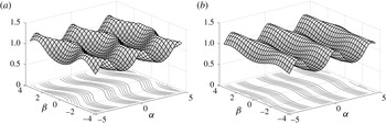
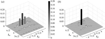
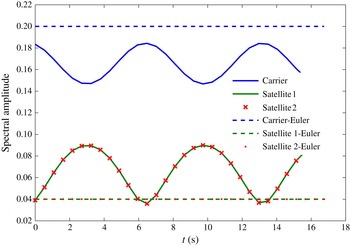
1. Introduction
The Lagrangian description of interactions between multiple surface gravity waves was pioneered by Pierson (Reference Pierson1961) half a century ago. Pierson explicitly derived a first-order solution for two-dimensional surfaces and pushed the calculation to the second order for long-crested surfaces. He showed that first-order results of a Lagrangian analysis included more realistic features than did using its Eulerian counterpart, such as sharp crests and flat troughs. In the present work, we revisit and correct this classical analysis to provide a general analytical framework, and to derive a compact and vectorial form of a second-order Lagrangian description of arbitrary tri-dimensional gravity wave fields. The analysis of tri-dimensional multiple wave systems is much richer than the analysis of long-crested surfaces or monochromatic waves as some geometrical and dynamical characteristics of the wave field can only be accounted for by considering interactions between different, non-aligned free wave vectors.
To date, exploration of the numerical and analytical possibilities offered by the Lagrangian formalism somehow have been overlooked. A renewed interest in Lagrangian approaches and their mathematical (Yakubovich & Zenkovich Reference Yakubovich and Zenkovich2001; Buldakov, Taylor & Taylor Reference Buldakov, Taylor and Taylor2006; Clamond Reference Clamond2007) or practical implications (Gjosund Reference Gjosund2003; Fouques, Krogstad & Myrhaug Reference Fouques, Krogstad and Myrhaug2006; Fouques & Stansberg Reference Fouques and Stansberg2009) has arisen and has provided the means to better evaluate the statistical and geometrical description of free surface and mass transport (Socquet-Juglard et al. Reference Socquet-Juglard, Dysthe, Trulsen, Krogstad and Liu2005; Lindgren Reference Lindgren2006; Aberg Reference Aberg2007; Aberg & Lindgren Reference Aberg and Lindgren2008; Nouguier, Guérin & Chapron Reference Nouguier, Guérin and Chapron2009; Hsu, Chen & Wang Reference Hsu, Chen and Wang2010; Hsu, Ng & Hwung Reference Hsu, Ng and Hwung2012). The underlying reason behind these remarkable properties is that the Lagrangian representation is clearly well-suited to the description of steep waves and is a very useful mathematical tool for the correct evaluation of statistical quantities (such as height, slope and curvature distribution) of random gravity wave fields at limited costs in terms of analytical complexity.
Our main finding is given by (4.47) which summarizes the Lagrangian expressions of second-order displacements of water particles and pressure in the whole fluid domain. The analysis is restricted to infinite depth but there is no conceptual difficulty in relaxing this assumption. Full consistency with the second-order Eulerian expansion of Longuet-Higgins (Reference Longuet-Higgins1963) is demonstrated. Pierson’s (Reference Pierson1961) original second-order Lagrangian solution for long-crested waves is discussed and adjusted to agree with both Longuet-Higgins (Reference Longuet-Higgins1963) and our own derivations. We further discuss two remarkable phenomena which are not captured by second-order Eulerian expansions. First, the formation of horseshoe patterns is identified as being the result of a non-isotropic drift current. Second, Benjamin–Feir modulational instability is also revealed to be inherently present in the second-order Lagrangian framework as a simple beat effect between two neighbouring harmonics instead of an energy exchange between carrier and sideband waves.
2. Eulerian versus Lagrangian expansions
We shall consider an incompressible fluid of constant density
 ${\it\rho}$
and of infinite depth, subject only to the restoring force of gravity (surface tension and viscosity are ignored). The pressure is set to a constant:
 $p_{a}$
at the free surface of the fluid. A fixed system of axes (
 $\widehat{\boldsymbol{x}},\widehat{\boldsymbol{y}},\widehat{\boldsymbol{z}}$
) with upwards-directed vertical vector
 $\widehat{\boldsymbol{z}}$
is chosen.
2.1. Eulerian description
In the Eulerian description, any position in space is identified by its coordinates
 $(x,y,z)$
, which can be decomposed into its horizontal projection
 $\boldsymbol{r}=(x,y)$
and vertical elevation
 $z$
. Under potential assumption, the evolving field of gravity waves is described by its elevations
 ${\it\eta}(\boldsymbol{r},t)$
and velocity potential
 $\underline{{\it\Phi}}(x,y,z,t)$
, with
 $t$
being the time variable. Under Eulerian coordinates the potential solves Laplace’s equation inside the volume together with dynamic and kinematic conditions at the borders:
 $$\begin{eqnarray}\left.\begin{array}{@{}c@{}}\displaystyle {\rm\Delta}\underline{{\it\Phi}}=0,\quad z<{\it\eta}(x,y,t)\\ \displaystyle \lim _{z\rightarrow -\infty }\boldsymbol{{\rm\nabla}}\underline{{\it\Phi}}=0,\\ \displaystyle \underline{{\it\Phi}}_{t}+{\textstyle \frac{1}{2}}\boldsymbol{{\rm\nabla}}\underline{{\it\Phi}}\boldsymbol{\cdot }\boldsymbol{{\rm\nabla}}\underline{{\it\Phi}}=-g{\it\eta},\quad z={\it\eta}(x,y,t)\\ \displaystyle \underline{{\it\Phi}}_{z}={\it\eta}_{t}+\boldsymbol{{\rm\nabla}}{\it\eta}\boldsymbol{\cdot }\boldsymbol{{\rm\nabla}}\underline{{\it\Phi}},\quad z={\it\eta}(x,y,t),\end{array}\right\}\end{eqnarray}$$
where
 $g$
is the acceleration due to gravity. System (2.1) describes potential waves. In the classical perturbative approach (Hasselmann Reference Hasselmann1962; Longuet-Higgins Reference Longuet-Higgins1963; Weber & Barrick Reference Weber and Barrick1977) the field of elevation
 ${\it\eta}$
and the velocity potential
 $\underline{{\it\Phi}}$
at the position and time
 $(\boldsymbol{r},t)$
are sought in the form
 $$\begin{eqnarray}\left.\begin{array}{@{}c@{}}{\it\eta}={\it\eta}_{0}+{\it\eta}_{1}+{\it\eta}_{2}+\cdots \\ \underline{{\it\Phi}}=\underline{{\it\Phi}}_{0}+\underline{{\it\Phi}}_{1}+\underline{{\it\Phi}}_{2}+\cdots \,.\end{array}\right\}\end{eqnarray}$$
The naught terms,
 ${\it\eta}_{0}$
and
 $\underline{{\it\Phi}}_{0}$
, are the reference solutions corresponding to a flat fluid interface and the next terms,
 ${\it\eta}_{1}$
and
 $\underline{{\it\Phi}}_{1}$
, are the solutions provided by the linearized equations. The successive terms,
 ${\it\eta}_{n}$
and
 $\underline{{\it\Phi}}_{n}$
, are
 $n$
th-order corrections with respect to one small parameter. In the general case of multiple waves, this small parameter is not well identified but in the case of a monochromatic wave it can be linked to the wave steepness.
2.2. Lagrangian description
In the Lagrangian approach (Lamb Reference Lamb1932), fluid evolution is described by the motion of fluid particles. The spatial coordinates
 $\boldsymbol{R}=(x,y,z)$
of the particles now depend on their independent reference labels
 ${\bf\zeta}=({\it\alpha},{\it\beta},{\it\delta})$
and time
 $t$
, that is explicitly
 $x=x({\it\alpha},{\it\beta},{\it\delta},t),y=y({\it\alpha},{\it\beta},{\it\delta},t)$
and
 $z=z({\it\alpha},{\it\beta},{\it\delta},t)$
. Hereafter
 ${\bf\zeta}$
is chosen to be the locus of particles at rest. For ease of reading we shall introduce dedicated notations for the horizontal component of particle labels and positions,
 ${\bf\xi}=({\it\alpha},{\it\beta})$
and
 $\boldsymbol{r}=(x,y)$
, respectively.
The evolution of particle coordinates is driven by Newton’s law of dynamics:
 $$\begin{eqnarray}\boldsymbol{R}_{tt}+g\widehat{\boldsymbol{z}}=-{\displaystyle \frac{1}{{\it\rho}}}\boldsymbol{{\rm\nabla}}_{\boldsymbol{R}}p\end{eqnarray}$$
where
 $p=p(\boldsymbol{R})$
is the local pressure. This dynamical equation is coupled with the continuity equation:
 $$\begin{eqnarray}|\mathbb{J}|=1;\quad {\displaystyle \frac{\partial }{\partial t}}|\mathbb{J}|=0\quad \text{with}~\mathbb{J}=\left[\begin{array}{@{}ccc@{}}x_{{\it\alpha}} & y_{{\it\alpha}} & z_{{\it\alpha}}\\ x_{{\it\beta}} & y_{{\it\beta}} & z_{{\it\beta}}\\ x_{{\it\delta}} & y_{{\it\delta}} & z_{{\it\delta}}\end{array}\right].\end{eqnarray}$$
Multiplying (2.3) by
 $\mathbb{J}$
gives
 $$\begin{eqnarray}\mathbb{J}\boldsymbol{R}_{tt}+g\boldsymbol{{\rm\nabla}}(\boldsymbol{R}\boldsymbol{\cdot }\widehat{\boldsymbol{z}})+{\displaystyle \frac{1}{{\it\rho}}}\boldsymbol{{\rm\nabla}}p=0\end{eqnarray}$$
which is the basic equation given by Lamb (Reference Lamb1932). From now on the spatial gradient relative to the independent Lagrangian variables
 $({\it\alpha},{\it\beta},{\it\delta})$
will be denoted by
 $\boldsymbol{{\rm\nabla}}$
.
Solutions to these equations need not be irrotational. However, if a function
 $F({\bf\zeta},t)$
can be found such that
 $$\begin{eqnarray}\text{d}F=(\mathbb{J}\boldsymbol{R}_{t})\boldsymbol{\cdot }\text{d}{\bf\zeta}\end{eqnarray}$$
is a perfect differential then there is no vorticity (see § A.1). Here
 $\text{d}{\bf\zeta}=(\text{d}{\it\alpha},\text{d}{\it\beta},\text{d}{\it\delta})$
denotes an infinitesimal label variation. Following the methodology described by Stoker (Reference Stoker1957) we may seek at solution in the form of a simultaneous perturbation expansion for position, pressure and the vorticity function:
 $$\begin{eqnarray}\left.\begin{array}{@{}c@{}}\boldsymbol{R}=\boldsymbol{R}_{0}+\boldsymbol{R}_{1}+\boldsymbol{R}_{2}+\cdots \\ p=p_{a}-{\it\rho}g{\it\delta}+p_{1}+p_{2}+\cdots \\ F=F_{0}+F_{1}+F_{2}+\cdots \end{array}\right\}\end{eqnarray}$$
where the naught variables refer to particles at rest.
3. First-order solution: the Gerstner wave
Let us map the fluid domain onto the half-space
 ${\it\delta}\leqslant 0$
. From now on,
 ${\it\delta}=0$
corresponds to the free surface
 ${\it\eta}$
under pressure
 $p_{a}$
. The zeroth-order solution to expansion (2.7) is related to particles at rest and can be written
 $$\begin{eqnarray}\left.\begin{array}{@{}c@{}}\boldsymbol{R}_{0}={\bf\zeta},\\ p_{0}=p_{a}-{\it\rho}g{\it\delta}\\ F_{0}=0\\ |\mathbb{J}|=1.\end{array}\right\}\end{eqnarray}$$
First-order quantities are solutions to linearized Lagrangian equations. When taken at the first order, equation (2.5) can be written
 $$\begin{eqnarray}\boldsymbol{R}_{1tt}+g\boldsymbol{{\rm\nabla}}(\boldsymbol{R}_{1}\boldsymbol{\cdot }\widehat{\boldsymbol{z}})+{\displaystyle \frac{1}{{\it\rho}}}\boldsymbol{{\rm\nabla}}p_{1}=0\end{eqnarray}$$
and the continuity equation is expressed by
 $$\begin{eqnarray}x_{1{\it\alpha}}+y_{1{\it\beta}}+z_{1{\it\delta}}=\boldsymbol{{\rm\nabla}}\boldsymbol{\cdot }\boldsymbol{R}_{1}=0.\end{eqnarray}$$
In order to simplify the calculations presented in the next section and to ensure an irrotational solution at the first order (see (3.9) below), we shall investigate solutions of the form
 $\boldsymbol{R}_{1}=\boldsymbol{{\rm\nabla}}w$
in an effort to see whether there exists a function for
 $w({\bf\zeta},t)$
. This last quantity must satisfy the following equation:
 $$\begin{eqnarray}\boldsymbol{{\rm\nabla}}(w_{tt}+gw_{{\it\delta}}+p_{1}/{\it\rho})=0.\end{eqnarray}$$
Setting
 $p_{1}$
to 0 at
 ${\it\delta}=0$
gives
 $$\begin{eqnarray}w=\cos (\boldsymbol{k}\boldsymbol{\cdot }{\bf\xi}-{\it\omega}t)\text{e}^{k{\it\delta}};\quad {\it\omega}^{2}=gk;\quad p_{1}=0\end{eqnarray}$$
where
 $\boldsymbol{k}=(k_{{\it\alpha}},k_{{\it\beta}})$
is an independent bi-dimensional vector in the
 $({\it\alpha},{\it\beta})$
domain and
 $k$
a constant parameter. At the first order in
 ${\it\epsilon}$
, the relation of continuity (3.3) can be written
 $$\begin{eqnarray}{\rm\Delta}w=(-k_{{\it\alpha}}^{2}-k_{{\it\beta}}^{2}+k^{2})w=0\end{eqnarray}$$
leading to
 $\Vert \boldsymbol{k}\Vert =k$
. As
 $\boldsymbol{R}_{1}$
is a spatial displacement, a suitable solution is
 $\boldsymbol{R}_{1}=\boldsymbol{{\rm\nabla}}(ak^{-1}w)$
which leads to the first-order solution:
 $$\begin{eqnarray}\left.\begin{array}{@{}c@{}}\boldsymbol{r}={\bf\xi}-a\widehat{\boldsymbol{k}}\sin (\boldsymbol{k}\boldsymbol{\cdot }{\bf\xi}-{\it\omega}t)\text{e}^{k{\it\delta}}\\ z={\it\delta}+a\cos (\boldsymbol{k}\boldsymbol{\cdot }{\bf\xi}-{\it\omega}t)\text{e}^{k{\it\delta}}\\ p=p_{0}-{\it\rho}g{\it\delta}.\end{array}\right\}\end{eqnarray}$$
From now on, we shall use the notation
 $\widehat{\boldsymbol{k}}=\boldsymbol{k}/k$
for the direction of a vector
 $\boldsymbol{k}$
and
 $k$
for its norm. This solution describes the trajectories of water particles as circles whose radii decrease exponentially with water depth. The spatial profile of such waves is a trochoid moving in the direction
 $\boldsymbol{k}$
with a crest to trough wave amplitude defined by
 $a$
, being the circle radius of the trajectories of particles at the free surface.
Two centuries ago, Gerstner (Reference Gerstner1809) derived an exact solution to the equation of motion (2.3) and obtained the same solution (3.7) for water particle trajectories
 $(\boldsymbol{r},z)$
with, however, a slightly different pressure term:
 $$\begin{eqnarray}p=p_{0}-{\it\rho}g{\it\delta}+{\textstyle \frac{1}{2}}k^{-2}{\it\rho}{\it\omega}^{2}\text{e}^{2k{\it\delta}}.\end{eqnarray}$$
The Gerstner wave has been described in classical textbooks (e.g. Lamb Reference Lamb1932; Kinsman Reference Kinsman1965) even though its stability was investigated only recently (Naciri & Mei Reference Naciri and Mei1992; Leblanc Reference Leblanc2004). It has always been criticized in view of its non-vanishing vorticity. This calls for some discussion on the presence of vorticity. Wind waves do in general exhibit vorticity, although it is in fact low. The main reason for which most of the studies have been devoted to irrotational waves is the considerable simplification offered by potential theory in the analytical derivations. It turns out that the predictions of potential theory agree reasonably well with observations, which does not mean that real waves are irrotational but rather that vorticity has only secondary effects. However, discrepancies are bound to become visible as the quality and accuracy of observations improve and it will soon become necessary to account for vorticity. The main shortcoming of the Gerstner solution is that it does not address a wide class of solutions with low vorticity. Its vorticity has in fact a very special distribution and there is no rationale for it to be more relevant than any other distribution of the same order. In the present analytical framework, the construction of a weakly nonlinear solution to the exact inviscid equations is more general and it is possible to examine arbitrary distributions with low vorticity and evaluate, at least coarsely, the importance of this effect.
As already derived by Pierson (Reference Pierson1961), equation (2.6) at first order in
 ${\it\epsilon}$
can be written
 $$\begin{eqnarray}\text{d}F=\boldsymbol{R}_{1t}\boldsymbol{\cdot }\text{d}{\bf\zeta}\end{eqnarray}$$
which is a perfect differential of
 $F_{1}$
since
 $\text{d}F=\boldsymbol{{\rm\nabla}}F_{1}\boldsymbol{\cdot }\text{d}{\bf\zeta}$
with
 $$\begin{eqnarray}F_{1}=ak^{-1}w_{t}={\displaystyle \frac{a{\it\omega}}{k}}\sin (\boldsymbol{k}\boldsymbol{\cdot }{\bf\xi}-{\it\omega}t)\text{e}^{k{\it\delta}}.\end{eqnarray}$$
Therefore, there is no vorticity at the first order and the Gerstner wave (with the corresponding pressure given by (3.7)) is an irrotational solution at the considered order of the expansion.
Owing to the linearity of (2.5), we can write an extended solution to the first-order equations as a continuous superposition of independent harmonics defined by their wavenumber
 $\boldsymbol{k}$
in the form:
 $$\begin{eqnarray}\boldsymbol{R}_{1}=\boldsymbol{{\rm\nabla}}{\it\Phi}_{1}\quad \text{with}~{\it\Phi}_{1}={\it\phi}_{1}+\text{c.c.},\end{eqnarray}$$
where ‘c.c.’ designates the complex conjugate of a given quantity and
 $$\begin{eqnarray}{\it\phi}_{1}={\displaystyle \frac{1}{2}}\int _{\mathbb{R}^{2}}{\displaystyle \frac{A(\boldsymbol{k})}{k}}\text{e}^{\text{i}(\boldsymbol{k}\boldsymbol{\cdot }{\bf\xi}-{\it\omega}t)}\text{e}^{k{\it\delta}}\text{d}\boldsymbol{k}.\end{eqnarray}$$
Here
 $A(\boldsymbol{k})$
is the orbital amplitude and the factor
 $1/2$
accounts for the complex plus conjugate formulation of
 ${\it\Phi}_{1}$
. Such an orbital spectrum has been already introduced in the statistical studies of Lagrangian wave fields (Pierson Reference Pierson1961; Daemrich & Woltering Reference Daemrich and Woltering2008; Lindgren & Lindgren Reference Lindgren and Lindgren2011) and describes the spectral content of particle motion. It is sometimes termed the ‘undressed’ spectrum (Elfouhaily et al.
Reference Elfouhaily, Thompson, Vandemark and Chapron1999) when it refers to a nonlinear transformation of an underlying linear surface (Creamer et al.
Reference Creamer, Henyey, Schult and Wright1989).
In the present state of knowledge, establishing the relationship between the orbital (Lagrangian) and the surface (Eulerian) spectrum is still an issue. When the amplitude
 $A(\boldsymbol{k})$
is taken to be a complex random variable with independent uniformly distributed random phases, the resulting function
 ${\it\phi}_{1}$
is a complex random Gaussian process by virtue of the law of large numbers. However, the random surface
 ${\it\eta}$
defined by the locus of particles at the free surface is no longer Gaussian. This implies that the corresponding distribution of elevation, slopes and curvatures distributions deviate from the normal distribution. Statistical properties of such random wave fields have been studied in detail (e.g. Pierson Reference Pierson1961; Gjosund Reference Gjosund2003; Aberg & Lindgren Reference Aberg and Lindgren2008; Lindgren & Aberg Reference Lindgren and Aberg2009; Nouguier et al.
Reference Nouguier, Guérin and Chapron2009; Lindgren & Lindgren Reference Lindgren and Lindgren2011) and have been found to be more consistent with ocean wave field measurements. A contrario, it should be noted that a first-order expansion in the Eulerian framework, which expresses the surface and its derivatives as a linear superposition of free harmonics, is bound to the Gaussian statistics.
4. Second-order Lagrangian solution
This section is devoted to the second-order Lagrangian expansion. We recall the corresponding equations and detail the calculations to derive the second-order displacements and the pressure terms as functions of the Lagrangian variables. To simplify notation we shall omit the integration elements (
 $\text{d}\boldsymbol{k},\text{d}\boldsymbol{k}^{\prime }$
) and domains (
 $\mathbb{R}^{2}$
and
 $\mathbb{R}^{2}\times \mathbb{R}^{2}$
) in the following single and double integrals.
4.1. Second-order equations
Retaining the second-order terms in (2.5) we obtain:
 $$\begin{eqnarray}\boldsymbol{R}_{2tt}+g\boldsymbol{{\rm\nabla}}z_{2}+\boldsymbol{{\rm\nabla}}p_{2}/{\it\rho}=-\unicode[STIX]{x1D643}({\it\Phi}_{1})\boldsymbol{{\rm\nabla}}{\it\Phi}_{1tt},\end{eqnarray}$$
where
 $\unicode[STIX]{x1D643}$
is the Hessian operator, that is the square matrix built with the second-order partial derivatives relative to the
 $({\it\alpha},{\it\beta},{\it\delta})$
variables:
 $$\begin{eqnarray}\unicode[STIX]{x1D643}({\it\Phi}_{1})=\left[\begin{array}{@{}ccc@{}}\partial _{{\it\alpha}{\it\alpha}}^{2} & \partial _{{\it\alpha}{\it\beta}}^{2} & \partial _{{\it\alpha}{\it\delta}}^{2}\\ \partial _{{\it\beta}{\it\alpha}}^{2} & \partial _{{\it\beta}{\it\beta}}^{2} & \partial _{{\it\beta}{\it\delta}}^{2}\\ \partial _{{\it\delta}{\it\alpha}}^{2} & \partial _{{\it\delta}{\it\beta}}^{2} & \partial _{{\it\delta}{\it\delta}}^{2}\end{array}\right]{\it\Phi}_{1}.\end{eqnarray}$$
For practical purposes we rewrite the right-hand side of (4.1) as
 $$\begin{eqnarray}-\!\unicode[STIX]{x1D643}({\it\Phi}_{1})\boldsymbol{{\rm\nabla}}{\it\Phi}_{1tt}=\boldsymbol{S}+\boldsymbol{T}\end{eqnarray}$$
with
 $$\begin{eqnarray}\displaystyle & \boldsymbol{S}=(S^{{\it\alpha}},S^{{\it\beta}},S^{{\it\delta}})=-\unicode[STIX]{x1D643}({\it\phi}_{1})\boldsymbol{{\rm\nabla}}{\it\phi}_{1tt}+\text{c.c.} & \displaystyle\end{eqnarray}$$
 $$\begin{eqnarray}\displaystyle & \boldsymbol{T}=(T^{{\it\alpha}},T^{{\it\beta}},T^{{\it\delta}})=-\unicode[STIX]{x1D643}({\it\phi}_{1})\boldsymbol{{\rm\nabla}}{\it\phi}_{1tt}^{\ast }+\text{c.c.} & \displaystyle\end{eqnarray}$$
 $\ast$
’ refers to the complex conjugate. Straightforward derivations given in § A.2 lead to
 $$\begin{eqnarray}\left.\begin{array}{@{}c@{}}\displaystyle (S^{{\it\alpha}},S^{{\it\beta}})=\iint {\mathcal{N}}gkk^{\prime }\frac{\text{i}}{2}(\widehat{\boldsymbol{k}}+\widehat{\boldsymbol{k}^{\prime }})+\text{c.c.}\\ \displaystyle S^{{\it\delta}}=\iint {\mathcal{N}}gkk^{\prime }+\text{c.c.}\end{array}\right\}\end{eqnarray}$$
and
 $$\begin{eqnarray}\left.\begin{array}{@{}c@{}}\displaystyle (T^{{\it\alpha}},T^{{\it\beta}})=\iint \underline{{\mathcal{N}}}\,gkk^{\prime }\frac{\text{i}}{2}(\widehat{\boldsymbol{k}}-\widehat{\boldsymbol{k}^{\prime }})+\text{c.c.}\\ \displaystyle T^{{\it\delta}}=\iint \underline{{\mathcal{N}}}\,gkk^{\prime }+\text{c.c.}\end{array}\right\}\end{eqnarray}$$
where the kernels
 ${\mathcal{N}}$
and
 $\underline{{\mathcal{N}}}$
depend on the variables
 $\boldsymbol{k},\boldsymbol{k}^{\prime },{\bf\xi}$
,
 ${\it\delta}$
and
 $t$
and are defined as follows:
 $$\begin{eqnarray}{\mathcal{N}}={\mathcal{B}}\text{e}^{-\text{i}({\it\omega}+{\it\omega}^{\prime })t}\text{e}^{(k+k^{\prime }){\it\delta}}\quad \text{and}\quad \underline{{\mathcal{N}}}=\underline{{\mathcal{B}}}\text{e}^{-\text{i}({\it\omega}-{\it\omega}^{\prime })t}\text{e}^{(k+k^{\prime }){\it\delta}}\end{eqnarray}$$
with
 $$\begin{eqnarray}\displaystyle & {\mathcal{B}}(\boldsymbol{k},\boldsymbol{k}^{\prime },{\bf\xi})={\textstyle \frac{1}{4}}(1-\widehat{\boldsymbol{k}}\boldsymbol{\cdot }\widehat{\boldsymbol{k}}^{\prime })A(\boldsymbol{k})A(\boldsymbol{k}^{\prime })\text{e}^{\text{i}(\boldsymbol{k}+\boldsymbol{k}^{\prime })\boldsymbol{\cdot }{\bf\xi}} & \displaystyle\end{eqnarray}$$
 $$\begin{eqnarray}\displaystyle & \underline{{\mathcal{B}}}(\boldsymbol{k},\boldsymbol{k}^{\prime },{\bf\xi})={\textstyle \frac{1}{4}}(1+\widehat{\boldsymbol{k}}\boldsymbol{\cdot }\widehat{\boldsymbol{k}}^{\prime })A(\boldsymbol{k})A^{\ast }(\boldsymbol{k}^{\prime })\text{e}^{\text{i}(\boldsymbol{k}-\boldsymbol{k}^{\prime })\boldsymbol{\cdot }{\bf\xi}}. & \displaystyle\end{eqnarray}$$
 $$\begin{eqnarray}x_{2{\it\alpha}}+y_{2{\it\beta}}+z_{2{\it\delta}}+{\it\Phi}_{1{\it\alpha}{\it\alpha}}{\it\Phi}_{1{\it\beta}{\it\beta}}+{\it\Phi}_{1{\it\alpha}{\it\alpha}}{\it\Phi}_{1{\it\delta}{\it\delta}}+{\it\Phi}_{1{\it\beta}{\it\beta}}{\it\Phi}_{1{\it\delta}{\it\delta}}-{\it\Phi}_{1{\it\alpha}{\it\beta}}^{2}-{\it\Phi}_{1{\it\alpha}{\it\delta}}^{2}-{\it\Phi}_{1{\it\beta}{\it\delta}}^{2}=0\end{eqnarray}$$
and can be rewritten in the form (see § A.3)
 $$\begin{eqnarray}\boldsymbol{{\rm\nabla}}\boldsymbol{\cdot }\boldsymbol{R}_{2}=V+W\end{eqnarray}$$
with
 $$\begin{eqnarray}V=\iint \frac{1}{2}(kk^{\prime }-\boldsymbol{k}\boldsymbol{\cdot }\boldsymbol{k}^{\prime }){\mathcal{N}}+\text{c.c.}\quad \text{and}\quad W=\iint \frac{1}{2}(kk^{\prime }+\boldsymbol{k}\boldsymbol{\cdot }\boldsymbol{k}^{\prime })\underline{{\mathcal{N}}}+\text{c.c.}\end{eqnarray}$$
4.2. Second-order expressions
Due to the linearity of (4.1) and (4.12), we shall first consider the solution to (4.1) with the sole
 $\boldsymbol{S}$
term on the right-hand side, that is,
 $$\begin{eqnarray}\boldsymbol{R}_{2tt}+g\boldsymbol{{\rm\nabla}}z_{2}+\boldsymbol{{\rm\nabla}}p_{2}/{\it\rho}=\boldsymbol{S}.\end{eqnarray}$$
We furthermore assume that
 $\boldsymbol{r}_{2},z_{2}$
and
 $p_{2}$
can be written as the following integrals:
 $$\begin{eqnarray}\displaystyle & \displaystyle \boldsymbol{r}_{2}=\iint {\mathcal{N}}\text{i}\,\boldsymbol{{\mathcal{R}}}+\text{c.c.} & \displaystyle\end{eqnarray}$$
 $$\begin{eqnarray}\displaystyle & \displaystyle z_{2}=\iint {\mathcal{N}}{\mathcal{Z}}+\text{c.c.} & \displaystyle\end{eqnarray}$$
 $$\begin{eqnarray}\displaystyle & \displaystyle p_{2}={\it\rho}g\iint {\mathcal{N}}{\mathcal{P}}+\text{c.c.}, & \displaystyle\end{eqnarray}$$
 $\boldsymbol{{\mathcal{R}}}$
,
 ${\mathcal{Z}}$
and
 ${\mathcal{P}}$
are unknown kernels depending on
 $\boldsymbol{k}$
and
 $\boldsymbol{k}^{\prime }$
. Inserting these expressions in (4.14) leads to a set of equations for the kernels:
 $$\begin{eqnarray}\left.\begin{array}{@{}c@{}}-{\mathcal{Z}}{\it\Omega}^{+}+({\mathcal{Z}}+{\mathcal{P}})(k+k^{\prime })=kk^{\prime }\\ -{\it\Omega}^{+}\boldsymbol{{\mathcal{R}}}+(\boldsymbol{k}+\boldsymbol{k}^{\prime })({\mathcal{Z}}+{\mathcal{P}})={\textstyle \frac{1}{2}}kk^{\prime }(\widehat{\boldsymbol{k}}+\widehat{\boldsymbol{k}^{\prime }}),\end{array}\right\}\end{eqnarray}$$
where we have defined
 $$\begin{eqnarray}{\it\Omega}^{\pm }=\left(\sqrt{k}\pm \sqrt{k^{\prime }}\right)^{2}.\end{eqnarray}$$
Inserting again (4.15)–(4.17) into (4.12) and keeping only the terms involving the kernel
 ${\mathcal{N}}$
leads to a third equation:
 $$\begin{eqnarray}-\boldsymbol{{\mathcal{R}}}\boldsymbol{\cdot }(\boldsymbol{k}+\boldsymbol{k}^{\prime })+{\mathcal{Z}}(k+k^{\prime })={\textstyle \frac{1}{2}}(kk^{\prime }-\boldsymbol{k}\boldsymbol{\cdot }\boldsymbol{k}^{\prime }).\end{eqnarray}$$
Equations (4.18) and (4.20) can easily be solved leading to
 $$\begin{eqnarray}\left.\begin{array}{@{}c@{}}\displaystyle \boldsymbol{{\mathcal{R}}}={\displaystyle \frac{{\it\omega}\boldsymbol{k}+{\it\omega}^{\prime }\boldsymbol{k}^{\prime }}{2({\it\omega}+{\it\omega}^{\prime })}}\\ {\mathcal{Z}}={\textstyle \frac{1}{4}}(k+k^{\prime }+{\it\Omega}^{-})\\ {\mathcal{P}}=\sqrt{kk^{\prime }}.\end{array}\right\}\end{eqnarray}$$
Analogously, we have to solve (4.1) with the sole term
 $\boldsymbol{T}$
on the right-hand side, which gives
 $$\begin{eqnarray}\boldsymbol{R}_{2tt}+g\boldsymbol{{\rm\nabla}}z_{2}+\boldsymbol{{\rm\nabla}}p_{2}/{\it\rho}=\boldsymbol{T}.\end{eqnarray}$$
Again, we assume that there exist
 $\boldsymbol{r}_{2},z_{2}$
and
 $p_{2}$
in the form given in (4.15)–(4.17) with some other kernels
 $\underline{{\mathcal{N}}}$
,
 $\underline{\boldsymbol{{\mathcal{R}}}}$
,
 $\underline{{\mathcal{Z}}}$
and
 $\underline{{\mathcal{P}}}$
. Since (4.12) involving the kernel
 ${\mathcal{N}}$
has already been solved, the only remaining terms are those involving
 $\underline{{\mathcal{N}}}$
in (4.12). A set of three equations is thus obtained for the unknown kernels:
 $$\begin{eqnarray}\left.\begin{array}{@{}c@{}}-\underline{{\mathcal{Z}}}{\it\Omega}^{-}+(\underline{{\mathcal{Z}}}+\underline{{\mathcal{P}}})(k+k^{\prime })=kk^{\prime }\\ -{\it\Omega}^{-}\underline{\boldsymbol{{\mathcal{R}}}}+(\boldsymbol{k}-\boldsymbol{k}^{\prime })(\underline{{\mathcal{Z}}}+\underline{{\mathcal{P}}})={\textstyle \frac{1}{2}}kk^{\prime }(\widehat{\boldsymbol{k}}-\widehat{\boldsymbol{k}^{\prime }})\\ -\underline{\boldsymbol{{\mathcal{R}}}}\boldsymbol{\cdot }(\boldsymbol{k}-\boldsymbol{k}^{\prime })+\underline{{\mathcal{Z}}}(k+k^{\prime })={\textstyle \frac{1}{2}}(kk^{\prime }+\boldsymbol{k}\boldsymbol{\cdot }\boldsymbol{k}^{\prime }).\end{array}\right\}\end{eqnarray}$$
Again, this system can easily be solved, leading to
 $$\begin{eqnarray}\left.\begin{array}{@{}c@{}}\displaystyle \underline{\boldsymbol{{\mathcal{R}}}}={\displaystyle \frac{{\it\omega}\boldsymbol{k}+{\it\omega}^{\prime }\boldsymbol{k}^{\prime }}{2({\it\omega}-{\it\omega}^{\prime })}}\\ \underline{{\mathcal{Z}}}={\textstyle \frac{1}{4}}(k+k^{\prime }+{\it\Omega}^{+})\\ \underline{{\mathcal{P}}}=-\sqrt{kk^{\prime }}\end{array}\right\}\quad \text{if }{\it\omega}\neq {\it\omega}^{\prime }.\end{eqnarray}$$
The case
 ${\it\omega}={\it\omega}^{\prime }$
will be discussed in detail in § 4.3. At this point we have found a solution to the second-order Lagrangian expansion (4.1) in the form
 $$\begin{eqnarray}\displaystyle & \displaystyle \boldsymbol{r}_{2}=\iint \text{i}({\mathcal{N}}\boldsymbol{{\mathcal{R}}}+\underline{{\mathcal{N}}}\,\underline{\boldsymbol{{\mathcal{R}}}})+\text{c.c.} & \displaystyle\end{eqnarray}$$
 $$\begin{eqnarray}\displaystyle & \displaystyle z_{2}=\iint \left({\mathcal{N}}{\mathcal{Z}}+\underline{{\mathcal{N}}}\,\underline{{\mathcal{Z}}}\right)+\text{c.c.} & \displaystyle\end{eqnarray}$$
 $$\begin{eqnarray}\displaystyle & \displaystyle p_{2}={\it\rho}g\iint \left({\mathcal{N}}{\mathcal{P}}+\underline{{\mathcal{N}}}\,\underline{{\mathcal{P}}}\right)+\text{c.c.} & \displaystyle\end{eqnarray}$$
However, the expression of
 $p_{2}$
does not satisfy the boundary condition
 $p_{2}=0$
at
 ${\it\delta}=0$
and needs to be corrected. Noting that
 ${\mathcal{N}}={\mathcal{B}}\text{e}^{-\text{i}({\it\omega}+{\it\omega}^{\prime })t}~\text{e}^{(k+k^{\prime }){\it\delta}}$
and
 $\underline{{\mathcal{N}}}=\underline{{\mathcal{B}}}\text{e}^{-\text{i}({\it\omega}-{\it\omega}^{\prime })t}~\text{e}^{(k+k^{\prime }){\it\delta}}$
, a very simple way to satisfy to the boundary condition is to complete
 $p_{2}$
in the form:
 $$\begin{eqnarray}p_{2}={\it\rho}g\iint {\mathcal{P}}{\mathcal{B}}\text{e}^{-\text{i}({\it\omega}+{\it\omega}^{\prime })t}(\text{e}^{(k+k^{\prime }){\it\delta}}-\text{e}^{K^{+}{\it\delta}})+\underline{{\mathcal{P}}}\underline{{\mathcal{B}}}\text{e}^{-\text{i}({\it\omega}-{\it\omega}^{\prime })t}(\text{e}^{(k+k^{\prime }){\it\delta}}-\text{e}^{K^{-}{\it\delta}})+\text{c.c.}\end{eqnarray}$$
where the additional kernels
 $K^{+}$
and
 $K^{-}$
must be determined. The pressure at the second order can thus be written as
 $$\begin{eqnarray}p_{2}=\iint (({\mathcal{N}}-{\mathcal{N}}^{\prime }){\mathcal{P}}+(\underline{{\mathcal{N}}}-\underline{{\mathcal{N}}}^{\prime })\underline{{\mathcal{P}}})+\text{c.c.}\end{eqnarray}$$
where we have introduced the two kernels
 ${\mathcal{N}}^{\prime }$
and
 $\underline{{\mathcal{N}}}^{\prime }$
, which only differ from
 ${\mathcal{N}}$
and
 $\underline{{\mathcal{N}}}$
, respectively, by the real exponential term:
 $$\begin{eqnarray}{\mathcal{N}}^{\prime }={\mathcal{B}}\text{e}^{-\text{i}({\it\omega}+{\it\omega}^{\prime })t}\text{e}^{K^{+}{\it\delta}}\quad \text{and}\quad \underline{{\mathcal{N}}}^{\prime }=\underline{{\mathcal{B}}}\text{e}^{-\text{i}({\it\omega}-{\it\omega}^{\prime })t}\text{e}^{K^{-}{\it\delta}}.\end{eqnarray}$$
It is therefore natural to assume a complete expression of
 $\boldsymbol{r}_{2}$
and
 $z_{2}$
in the form
 $$\begin{eqnarray}\displaystyle & \displaystyle \boldsymbol{r}_{2}=\iint \text{i}({\mathcal{N}}\boldsymbol{{\mathcal{R}}}-{\mathcal{N}}^{\prime }\boldsymbol{{\mathcal{R}}}^{\prime }+\underline{{\mathcal{N}}}\,\underline{\boldsymbol{{\mathcal{R}}}}-\underline{{\mathcal{N}}}^{\prime }\underline{\boldsymbol{{\mathcal{R}}}^{\prime }})+\text{c.c.} & \displaystyle\end{eqnarray}$$
 $$\begin{eqnarray}\displaystyle & \displaystyle z_{2}=\iint ({\mathcal{N}}{\mathcal{Z}}-{\mathcal{N}}^{\prime }{\mathcal{Z}}^{\prime }+\underline{{\mathcal{N}}}\,\underline{{\mathcal{Z}}}-\underline{{\mathcal{N}}}^{\prime }\underline{{\mathcal{Z}}^{\prime }})+\text{c.c.}, & \displaystyle\end{eqnarray}$$
 ${\mathcal{N}}^{\prime }$
kernel only. This leads to the following equations:
 $$\begin{eqnarray}\displaystyle & -{\it\Omega}^{+}{\mathcal{Z}}^{\prime }+K^{+}({\mathcal{Z}}^{\prime }+P)=0 & \displaystyle\end{eqnarray}$$
 $$\begin{eqnarray}\displaystyle & -{\it\Omega}^{+}\boldsymbol{{\mathcal{R}}}^{\prime }+(\boldsymbol{k}+\boldsymbol{k}^{\prime })({\mathcal{Z}}^{\prime }+P)=0, & \displaystyle\end{eqnarray}$$
 $$\begin{eqnarray}-\boldsymbol{{\mathcal{R}}}^{\prime }\boldsymbol{\cdot }(\boldsymbol{k}+\boldsymbol{k}^{\prime })+K^{+}{\mathcal{Z}}^{\prime }=0\end{eqnarray}$$
from the continuity equation. Inserting (4.33) into (4.34) and multiplying by
 $(\boldsymbol{k}+\boldsymbol{k}^{\prime })/{\it\Omega}^{+}$
leads to
 $$\begin{eqnarray}-\boldsymbol{{\mathcal{R}}}^{\prime }\boldsymbol{\cdot }(\boldsymbol{k}+\boldsymbol{k}^{\prime })+{\displaystyle \frac{\Vert \boldsymbol{k}+\boldsymbol{k}^{\prime }\Vert ^{2}}{K^{+}}}{\mathcal{Z}}^{\prime }=0\end{eqnarray}$$
which is consistent with (4.35) if and only if
 $$\begin{eqnarray}K^{+}=\Vert \boldsymbol{k}+\boldsymbol{k}^{\prime }\Vert\end{eqnarray}$$
(we discard the mathematical solution
 $K^{+}=-\Vert \boldsymbol{k}+\boldsymbol{k}^{\prime }\Vert$
which is non-physical because of the asymptotic constraint
 $p_{2}\rightarrow 0$
when
 ${\it\delta}\rightarrow -\infty$
). We can now solve (4.33) and (4.34) to obtain
 $$\begin{eqnarray}\left.\begin{array}{@{}c@{}}\displaystyle \boldsymbol{{\mathcal{R}}}^{\prime }={\displaystyle \frac{\sqrt{kk^{\prime }}(\boldsymbol{k}+\boldsymbol{k}^{\prime })}{{\it\Omega}^{+}-\Vert \boldsymbol{k}+\boldsymbol{k}^{\prime }\Vert }}\\ \displaystyle {\mathcal{Z}}^{\prime }={\displaystyle \frac{\sqrt{kk^{\prime }}\Vert \boldsymbol{k}+\boldsymbol{k}^{\prime }\Vert }{{\it\Omega}^{+}-\Vert \boldsymbol{k}+\boldsymbol{k}^{\prime }\Vert }}.\end{array}\right\}\end{eqnarray}$$
Repeating the same procedure with the kernel
 $\underline{{\mathcal{N}}}^{\prime }$
leads to another set of equations:
 $$\begin{eqnarray}\left.\begin{array}{@{}c@{}}-{\it\Omega}^{-}\underline{{\mathcal{Z}}^{\prime }}+K^{-}(\underline{{\mathcal{Z}}^{\prime }}+\underline{P})=0\\ -{\it\Omega}^{-}\underline{\boldsymbol{{\mathcal{R}}}^{\prime }}+(\boldsymbol{k}-\boldsymbol{k}^{\prime })(\underline{{\mathcal{Z}}^{\prime }}+\underline{P})=0\\ -\underline{\boldsymbol{{\mathcal{R}}}^{\prime }}\boldsymbol{\cdot }(\boldsymbol{k}-\boldsymbol{k}^{\prime })+K^{-}\underline{{\mathcal{Z}}^{\prime }}=0\end{array}\right\}\end{eqnarray}$$
which admit the solution
 $K^{-}=\Vert \boldsymbol{k}-\boldsymbol{k}^{\prime }\Vert$
and
 $$\begin{eqnarray}\left.\begin{array}{@{}c@{}}\displaystyle \underline{\boldsymbol{{\mathcal{R}}}^{\prime }}={\displaystyle \frac{-\sqrt{kk^{\prime }}(\boldsymbol{k}-\boldsymbol{k}^{\prime })}{{\it\Omega}^{-}-\Vert \boldsymbol{k}-\boldsymbol{k}^{\prime }\Vert }}\\ \displaystyle \underline{{\mathcal{Z}}^{\prime }}={\displaystyle \frac{-\sqrt{kk^{\prime }}\Vert \boldsymbol{k}-\boldsymbol{k}^{\prime }\Vert }{{\it\Omega}^{-}-\Vert \boldsymbol{k}-\boldsymbol{k}^{\prime }\Vert }}.\end{array}\right\}\end{eqnarray}$$
4.3. Interaction of harmonics of equal frequencies
The complete kernels involved in the integral representation of
 $\boldsymbol{R}_{2}$
and
 $p_{2}$
have now been found. However, in order to complete the solution to the second-order Lagrangian equations we need to discuss the case
 ${\it\omega}={\it\omega}^{\prime }$
which was initially discarded in (4.24).
A generalized expression of the horizontal second-order term corresponding to kernel solutions (4.24) for the case
 ${\it\omega}={\it\omega}^{\prime }$
would be written as the limit
 $$\begin{eqnarray}\underline{\boldsymbol{r}}_{2}=\lim _{{\it\gamma}\rightarrow 0}\iint _{\mathbb{R}^{4}-{\mathcal{E}}}\text{i}\underline{\boldsymbol{{\mathcal{R}}}}\underline{{\mathcal{N}}}+\text{c.c.}\end{eqnarray}$$
where
 ${\mathcal{E}}$
is the
 $\mathbb{R}^{4}$
subdomain so that
 $|{\it\omega}-{\it\omega}^{\prime }|<{\it\gamma}$
and where
 $\underline{\boldsymbol{{\mathcal{R}}}}$
, defined at (4.24), contains a singularity at
 ${\it\omega}={\it\omega}^{\prime }$
.
If this integral were to admit a finite value, it would have to be defined in the sense of Cauchy principal value (PV):
 $$\begin{eqnarray}\underline{\boldsymbol{r}}_{2}=\text{PV}\iint _{\mathbb{R}^{4}}\text{i}{\displaystyle \frac{{\it\omega}\boldsymbol{k}+{\it\omega}^{\prime }\boldsymbol{k}^{\prime }}{2({\it\omega}-{\it\omega}^{\prime })}}\underline{{\mathcal{B}}}\text{e}^{-\text{i}({\it\omega}-{\it\omega}^{\prime })t}\text{e}^{(k+k^{\prime }){\it\delta}}+\text{c.c.}\end{eqnarray}$$
The existence of the finite limit (4.41) is shown in appendix B ensuring that (4.42) is the correct expression of
 $\underline{\boldsymbol{r}}_{2}$
.
4.4. Second-order vorticity
A complete Lagrangian second-order solution has now been found. We can verify a posteriori that it is indeed irrotational. For this, we have to investigate the second-order expression of the function
 $\text{d}F$
, that is,
 $$\begin{eqnarray}\text{d}F_{2}=\left[\boldsymbol{R}_{2t}+\unicode[STIX]{x1D643}({\it\Phi}_{1})\boldsymbol{{\rm\nabla}}({\it\Phi}_{1t})\right]\boldsymbol{\cdot }\text{d}{\bf\zeta},\end{eqnarray}$$
which we chose to rewrite in the form
 $$\begin{eqnarray}\text{d}F_{2}=\int _{t}\,\text{d}t\left[\boldsymbol{R}_{2tt}+\unicode[STIX]{x1D643}({\it\Phi}_{1})\boldsymbol{{\rm\nabla}}({\it\Phi}_{1tt})+\unicode[STIX]{x1D643}({\it\Phi}_{1t})\boldsymbol{{\rm\nabla}}({\it\Phi}_{1t})\right]\boldsymbol{\cdot }\text{d}{\bf\zeta}\end{eqnarray}$$
where the symbol
 $\int _{t}\,\text{d}t$
refers to temporal integration. Inserting (4.1) into this last expression leads to
 $$\begin{eqnarray}\text{d}F_{2}=\boldsymbol{{\rm\nabla}}\left[\int _{t}\,\text{d}t\left(-(gz_{2}+p_{2}/{\it\rho})+\frac{1}{2}({\it\Phi}_{1t})^{2}\right)\right]\boldsymbol{\cdot }\text{d}{\bf\zeta}.\end{eqnarray}$$
This provides
 $F_{2}$
in the form:
 $$\begin{eqnarray}F_{2}=\int _{t}\,\text{d}t\left(\frac{1}{2}({\it\Phi}_{1t})^{2}-gz_{2}-p_{2}/{\it\rho}\right).\end{eqnarray}$$
The existence of such a function
 $F_{2}$
warrants the absence of vorticity at the second order.
4.5. Second-order solution
To summarize all of the expressions established previously, the general solution to the second-order terms of (2.7) can be written as follows:
 $$\begin{eqnarray}\left.\begin{array}{@{}rcl@{}}\boldsymbol{r}_{2}\, & =\, & \displaystyle \iint \text{i}\left({\displaystyle \frac{{\it\omega}\boldsymbol{k}+{\it\omega}^{\prime }\boldsymbol{k}^{\prime }}{2({\it\omega}+{\it\omega}^{\prime })}}\text{e}^{(k+k^{\prime }){\it\delta}}-{\displaystyle \frac{\sqrt{kk^{\prime }}(\boldsymbol{k}+\boldsymbol{k}^{\prime })}{{\it\Omega}^{+}-\Vert \boldsymbol{k}+\boldsymbol{k}^{\prime }\Vert }}\text{e}^{\Vert \boldsymbol{k}+\boldsymbol{k}^{\prime }\Vert {\it\delta}}\right){\mathcal{B}}\text{e}^{-\text{i}({\it\omega}+{\it\omega}^{\prime })t}+\text{c.c.}\\ \, & \, & +\,\displaystyle \text{PV}\iint \text{i}\left({\displaystyle \frac{{\it\omega}\boldsymbol{k}+{\it\omega}^{\prime }\boldsymbol{k}^{\prime }}{2({\it\omega}-{\it\omega}^{\prime })}}\text{e}^{(k+k^{\prime }){\it\delta}}+{\displaystyle \frac{\sqrt{kk^{\prime }}(\boldsymbol{k}-\boldsymbol{k}^{\prime })}{{\it\Omega}^{-}-\Vert \boldsymbol{k}-\boldsymbol{k}^{\prime }\Vert }}\text{e}^{\Vert \boldsymbol{k}-\boldsymbol{k}^{\prime }\Vert {\it\delta}}\right)\underline{{\mathcal{B}}}\text{e}^{-\text{i}({\it\omega}-{\it\omega}^{\prime })t}+\text{c.c.}\\ z_{2}\, & =\, & \displaystyle \iint \left({\displaystyle \frac{k+k^{\prime }+{\it\Omega}^{-}}{4}}\text{e}^{(k+k^{\prime }){\it\delta}}-{\displaystyle \frac{\sqrt{kk^{\prime }}\Vert \boldsymbol{k}+\boldsymbol{k}^{\prime }\Vert }{{\it\Omega}^{+}-\Vert \boldsymbol{k}+\boldsymbol{k}^{\prime }\Vert }}\text{e}^{\Vert \boldsymbol{k}+\boldsymbol{k}^{\prime }\Vert {\it\delta}}\right){\mathcal{B}}\text{e}^{-\text{i}({\it\omega}+{\it\omega}^{\prime })t}+\text{c.c.}\\ \, & \, & +\,\displaystyle \iint \left({\displaystyle \frac{k+k^{\prime }+{\it\Omega}^{+}}{4}}\text{e}^{(k+k^{\prime }){\it\delta}}+{\displaystyle \frac{\sqrt{kk^{\prime }}\Vert \boldsymbol{k}-\boldsymbol{k}^{\prime }\Vert }{{\it\Omega}^{-}-\Vert \boldsymbol{k}-\boldsymbol{k}^{\prime }\Vert }}\text{e}^{\Vert \boldsymbol{k}-\boldsymbol{k}^{\prime }\Vert {\it\delta}}\right)\underline{{\mathcal{B}}}\text{e}^{-\text{i}({\it\omega}-{\it\omega}^{\prime })t}+\text{c.c.}\\ p_{2}\, & =\, & \displaystyle {\it\rho}g\iint \sqrt{kk^{\prime }}\left(\text{e}^{(k+k^{\prime }){\it\delta}}-\text{e}^{\Vert \boldsymbol{k}+\boldsymbol{k}^{\prime }\Vert {\it\delta}}\right){\mathcal{B}}\text{e}^{-\text{i}({\it\omega}+{\it\omega}^{\prime })t}+\text{c.c.}\\ \, & \, & -\,\displaystyle {\it\rho}g\iint \sqrt{kk^{\prime }}\left(\text{e}^{(k+k^{\prime }){\it\delta}}-\text{e}^{\Vert \boldsymbol{k}-\boldsymbol{k}^{\prime }\Vert {\it\delta}}\right)\underline{{\mathcal{B}}}\text{e}^{-\text{i}({\it\omega}-{\it\omega}^{\prime })t}+\text{c.c.}\end{array}\right\}\end{eqnarray}$$
where
 ${\mathcal{B}}$
and
 $\underline{{\mathcal{B}}}$
are defined in (4.9) and (4.10) and
 ${\it\Omega}^{\pm }$
in (4.19).
5. Comparison with classical models
5.1. Consistency with the Eulerian approach of M. S. Longuet-Higgins
Before investigating the consistency of this model with classical Eulerian models, it is instructive to establish the correspondence between Eulerian and Lagrangian expansions. Let us consider the surface
 ${\it\eta}(\boldsymbol{r},t)$
implicitly defined by the locus of particle trajectories
 $(\boldsymbol{r}(t),z(t))$
and denote
 ${\it\eta}={\it\eta}_{0}+{\it\eta}_{1}+{\it\eta}_{2}+\cdots \,$
as its Eulerian expansion in order of steepness above a reference plane. Applying successive Taylor expansions and making use of the correspondence between the
 $({\it\alpha},{\it\beta},{\it\delta})$
Lagrangian labels and the
 $(x,y,z)$
coordinate system of the Eulerian description, it can be easily shown that
 $$\begin{eqnarray}\left.\begin{array}{@{}c@{}}{\it\eta}_{0}=z_{0}\\ {\it\eta}_{1}=z_{1}-\boldsymbol{r}_{1}\boldsymbol{\cdot }\boldsymbol{{\rm\nabla}}_{{\bf\xi}}{\it\eta}_{0}\\ {\it\eta}_{2}=z_{2}-\boldsymbol{r}_{1}\boldsymbol{\cdot }\boldsymbol{{\rm\nabla}}_{{\bf\xi}}{\it\eta}_{1}-\boldsymbol{r}_{2}\boldsymbol{\cdot }\boldsymbol{{\rm\nabla}}_{{\bf\xi}}{\it\eta}_{0}-{\textstyle \frac{1}{2}}\boldsymbol{r}_{1}\boldsymbol{{\rm\nabla}}_{{\bf\xi}}\boldsymbol{{\rm\nabla}}_{{\bf\xi}}{\it\eta}_{0}\boldsymbol{r}_{1}\\ {\it\eta}_{n}=z_{n}-\cdots \end{array}\right\}\end{eqnarray}$$
where
 $\boldsymbol{{\rm\nabla}}_{{\bf\xi}}$
is the horizontal bi-dimensional gradient and
 $\boldsymbol{{\rm\nabla}}_{{\bf\xi}}\boldsymbol{{\rm\nabla}}_{{\bf\xi}}$
the corresponding Hessian. The expansion can in principle be pursued at an arbitrary order even though it becomes algebraically more complex. From this it can seen than any
 $n$
th-order term in the surface elevation (
 ${\it\eta}_{n}$
) can be obtained from the combination of an
 $n$
th-order term in the vertical particle position (
 $z_{n}$
) and lower-order terms
 $(\boldsymbol{r}_{p},z_{p}),p\leqslant n-1$
. Hence, any given order of the Lagrangian expansion provides the complete corresponding Eulerian order and is moreover involved in higher-order Eulerian terms.
The classical Eulerian approach (Hasselmann Reference Hasselmann1962; Longuet-Higgins Reference Longuet-Higgins1963) to the nonlinear theory of gravity waves consist in seeking both the elevation
 ${\it\eta}$
and the velocity potential
 $\underline{{\it\Phi}}$
at the free surface in a perturbation series (2.2). The expansion is usually performed about the mean horizontal plane of the leading order
 ${\it\eta}_{0}$
so that no zeroth-order term is present:
 $$\begin{eqnarray}\displaystyle & {\it\eta}({\bf\xi},t)={\it\eta}_{1}({\bf\xi},t)+{\it\eta}_{2}({\bf\xi},t)+\cdots & \displaystyle\end{eqnarray}$$
 $$\begin{eqnarray}\displaystyle & \underline{{\it\Phi}}({\bf\xi},t)=\underline{{\it\Phi}}_{1}({\bf\xi},t)+\underline{{\it\Phi}}_{2}({\bf\xi},t)+\cdots \,. & \displaystyle\end{eqnarray}$$
 $(x,y)$
has been simply replaced by the
 $({\it\alpha},{\it\beta})$
system. The first-order terms are given by the classical spectral representation,
 $$\begin{eqnarray}\displaystyle & \displaystyle {\it\eta}_{1}({\bf\xi},t)=\mathop{\sum }_{j=1}^{N}a_{j}\cos {\it\psi}_{j},\quad {\it\psi}_{j}=\boldsymbol{k}_{\boldsymbol{j}}\boldsymbol{\cdot }{\bf\xi}-{\it\omega}_{j}t+{\it\varphi}_{j} & \displaystyle\end{eqnarray}$$
 $$\begin{eqnarray}\displaystyle & \displaystyle {\it\Phi}_{1}({\bf\xi},t)=\mathop{\sum }_{j=1}^{N}b_{j}\cos {\it\psi}_{j}, & \displaystyle\end{eqnarray}$$
where
 ${\it\varphi}_{j}$
is the phase associated to the
 $\boldsymbol{k}_{j}$
component. The higher-order terms in the expansion involve
 $n$
th-order multiplicative combinations of these spectral components. The perturbation expansions of elevation and velocity potential are identified simultaneously by injecting the successive Fourier expansions in Navier–Stokes equations. The leading, quadratic, nonlinear term for elevation was provided by Longuet-Higgins (Reference Longuet-Higgins1963) in the form
 $$\begin{eqnarray}\displaystyle & \displaystyle {\it\eta}_{2}({\bf\xi},t)=\frac{1}{2}\mathop{\sum }_{i,j=1}^{N}a_{i}a_{j}[K_{ij}\cos {\it\psi}_{i}\cos {\it\psi}_{j}+K_{ij}^{\prime }\sin {\it\psi}_{i}\sin {\it\psi}_{j}], & \displaystyle\end{eqnarray}$$
 $$\begin{eqnarray}\displaystyle & \displaystyle K_{ij}=(k_{i}k_{j})^{-1/2}[B_{ij}^{-}+B_{ij}^{+}-\boldsymbol{k}_{\boldsymbol{i}}\boldsymbol{\cdot }\boldsymbol{k}_{\boldsymbol{j}}]+k_{i}+k_{j} & \displaystyle\end{eqnarray}$$
 $$\begin{eqnarray}\displaystyle & \displaystyle K_{ij}^{\prime }=(k_{i}k_{j})^{-1/2}\left[B_{ij}^{-}-B_{ij}^{+}-k_{i}k_{j}\right] & \displaystyle\end{eqnarray}$$
 $$\begin{eqnarray}\displaystyle & \displaystyle B_{ij}^{\pm }={\displaystyle \frac{{\it\Omega}_{ij}^{\pm }(\boldsymbol{k}_{\boldsymbol{ i}}\boldsymbol{\cdot }\boldsymbol{k}_{\boldsymbol{j}}\mp k_{i}k_{j})}{{\it\Omega}_{ij}^{\pm }-\Vert \boldsymbol{k}_{i}\pm \boldsymbol{k}_{j}\Vert }} & \displaystyle\end{eqnarray}$$
 $$\begin{eqnarray}\displaystyle & {\it\Omega}_{ij}^{\pm }=(\sqrt{k_{i}}\pm \sqrt{k_{j}})^{2} & \displaystyle\end{eqnarray}$$
 $k=\Vert \boldsymbol{k}\Vert$
. (Note that the factor
 $1/2$
is missing in the original paper by Longuet-Higgins, as was later acknowledged by the author himself.) The first-order Lagrangian expansion was shown to be close but not perfectly consistent with the second-order Eulerian perturbation expansion of Longuet-Higgins (see Nouguier et al.
Reference Nouguier, Guérin and Chapron2009). We will now show that full consistency is achieved with Longuet-Higgins approach with the second-order Lagrangian expansion at the surface, that is,
 $$\begin{eqnarray}\left.\begin{array}{@{}c@{}}{\it\eta}_{1}=z_{1}\\ {\it\eta}_{2}=z_{2}-\boldsymbol{r}_{1}\boldsymbol{\cdot }\boldsymbol{{\rm\nabla}}_{{\bf\xi}}z_{1}\end{array}\right\}\end{eqnarray}$$
where, again,
 $\boldsymbol{{\rm\nabla}}_{{\bf\xi}}$
is the horizontal bi-dimensional gradient. It should be noted from (5.11) that
 $\boldsymbol{r}_{2}$
is absent emphasizing that the second-order Eulerian formalism misses all effects related to
 $\boldsymbol{r}_{2}$
contribution.
From (4.47), we have at the free surface (
 ${\it\delta}=0$
)
 $$\begin{eqnarray}\displaystyle z_{2} & = & \displaystyle {\displaystyle \frac{1}{2}}\iint \left\{\left({\displaystyle \frac{k+k^{\prime }+{\it\Omega}^{-}}{4}}-{\displaystyle \frac{\sqrt{kk^{\prime }}\Vert \boldsymbol{k}+\boldsymbol{k}^{\prime }\Vert }{{\it\Omega}^{+}-\Vert \boldsymbol{k}+\boldsymbol{k}^{\prime }\Vert }}\right)(1-\widehat{\boldsymbol{k}}\boldsymbol{\cdot }\widehat{\boldsymbol{k}}^{\prime })a_{\boldsymbol{ k}}a_{\boldsymbol{k}^{\prime }}\cos ({\it\psi}+{\it\psi}^{\prime })\right.\nonumber\\ \displaystyle & & \displaystyle \left.+\,\left({\displaystyle \frac{k+k^{\prime }+{\it\Omega}^{+}}{4}}+{\displaystyle \frac{\sqrt{kk^{\prime }}\Vert \boldsymbol{k}-\boldsymbol{k}^{\prime }\Vert }{{\it\Omega}^{-}-\Vert \boldsymbol{k}-\boldsymbol{k}^{\prime }\Vert }}\right)(1+\widehat{\boldsymbol{k}}\boldsymbol{\cdot }\widehat{\boldsymbol{k}}^{\prime })a_{\boldsymbol{ k}}a_{\boldsymbol{k}^{\prime }}\cos ({\it\psi}-{\it\psi}^{\prime })\right\}\end{eqnarray}$$
with
 $a_{\boldsymbol{k}}=\Vert A(\boldsymbol{k})\Vert$
and
 ${\it\psi}=\boldsymbol{k}\boldsymbol{\cdot }{\bf\xi}-{\it\omega}t+{\it\varphi}_{\boldsymbol{k}}$
where
 ${\it\varphi}_{\boldsymbol{k}}$
is the phase of
 $A(\boldsymbol{k})$
. Following some basic algebra
 $z_{2}$
can be rewritten in the form
 $$\begin{eqnarray}z_{2}={\displaystyle \frac{1}{2}}\iint a_{\boldsymbol{k}}a_{\boldsymbol{k}^{\prime }}\left[K\cos ({\it\psi})\cos ({\it\psi}^{\prime })+\left(K^{\prime }+\boldsymbol{k}^{\prime }\boldsymbol{\cdot }\widehat{\boldsymbol{k}}+\boldsymbol{k}\boldsymbol{\cdot }\widehat{\boldsymbol{k}}^{\prime }\right)\sin ({\it\psi})\sin ({\it\psi}^{\prime })\right]\end{eqnarray}$$
where kernels
 $K$
and
 $K^{\prime }$
are the continuous version of kernels
 $K_{ij}$
and
 $K_{ij}^{\prime }$
of (5.7) wherein the subscripts
 $i$
and
 $j$
are related to non-primed and primed variables.
To complete the expression (5.11) we observe that
 $$\begin{eqnarray}\displaystyle -\boldsymbol{r}_{1}\boldsymbol{\cdot }\boldsymbol{{\rm\nabla}}_{{\bf\xi}}{\it\eta}_{1}|_{{\it\delta}=0} & = & \displaystyle -\boldsymbol{{\rm\nabla}}_{{\bf\xi}}({\it\Phi}_{1})\boldsymbol{\cdot }\boldsymbol{{\rm\nabla}}_{{\bf\xi}}({\it\Phi}_{1{\it\delta}})|_{{\it\delta}=0}\nonumber\\ \displaystyle & = & \displaystyle -\iint (\boldsymbol{k}^{\prime }\boldsymbol{\cdot }\widehat{\boldsymbol{k}})a_{\boldsymbol{k}}a_{\boldsymbol{k}^{\prime }}\sin ({\it\psi})\sin ({\it\psi}^{\prime })\nonumber\\ \displaystyle & = & \displaystyle -\iint {\displaystyle \frac{1}{2}}(\boldsymbol{k}^{\prime }\boldsymbol{\cdot }\widehat{\boldsymbol{k}}+\boldsymbol{k}\boldsymbol{\cdot }\widehat{\boldsymbol{k}}^{\prime })a_{\boldsymbol{ k}}a_{\boldsymbol{k}^{\prime }}\sin ({\it\psi})\sin ({\it\psi}^{\prime }).\end{eqnarray}$$
The combination of (5.13) and (5.14) yields
 $$\begin{eqnarray}{\it\eta}_{2}={\displaystyle \frac{1}{2}}\iint a_{\boldsymbol{k}}a_{\boldsymbol{k}^{\prime }}[K\cos ({\it\psi})\cos ({\it\psi}^{\prime })+K^{\prime }\sin ({\it\psi})\sin ({\it\psi}^{\prime })],\end{eqnarray}$$
which is the continuous version of (5.6) derived by Longuet-Higgins (Reference Longuet-Higgins1963).
5.2. Consistency with the Lagrangian derivation of W. J. Pierson
In 1961 W. J. Pierson derived a Lagrangian second-order solution to the discrete long-crested problem. He considered waves travelling in the positive
 ${\it\alpha}$
direction only and found the solutions in the forms (equations (27) and (28) in Pierson (Reference Pierson1961)):
 $$\begin{eqnarray}\displaystyle x({\it\alpha},{\it\delta},t) & = & \displaystyle {\it\alpha}-\mathop{\sum }_{i}a_{i}\text{e}^{k_{i}{\it\delta}}\sin ({\it\psi}_{i})-\mathop{\sum }_{j>i}\mathop{\sum }_{i}{\displaystyle \frac{a_{i}a_{j}}{g}}\left({\displaystyle \frac{{\it\omega}_{i}^{3}+{\it\omega}_{j}^{3}}{{\it\omega}_{j}-{\it\omega}_{i}}}\right)\text{e}^{(k_{j}+k_{i}){\it\delta}}\sin ({\it\psi}_{j}-{\it\psi}_{i})\nonumber\\ \displaystyle & & \displaystyle +\,\mathop{\sum }_{j>i}\mathop{\sum }_{i}{\displaystyle \frac{a_{i}a_{j}}{g}}({\it\omega}_{j}+{\it\omega}_{i}){\it\omega}_{j}\text{e}^{(k_{j}-k_{i}){\it\delta}}\sin ({\it\psi}_{j}-{\it\psi}_{i})+\mathop{\sum }_{i}a_{i}^{2}{\it\omega}_{i}k_{i}\text{e}^{2k_{i}{\it\delta}}t\end{eqnarray}$$
 $$\begin{eqnarray}\displaystyle z({\it\alpha},{\it\delta},t) & = & \displaystyle {\it\delta}+\mathop{\sum }_{i}a_{i}\text{e}^{k_{i}{\it\delta}}\cos ({\it\psi}_{i})+\mathop{\sum }_{j>i}\mathop{\sum }_{i}{\displaystyle \frac{a_{i}a_{j}}{g}}({\it\omega}_{i}^{2}+{\it\omega}_{i}{\it\omega}_{j}+{\it\omega}_{j}^{2})\text{e}^{(k_{j}+k_{i}){\it\delta}}\nonumber\\ \displaystyle & & \displaystyle \times \,\cos ({\it\psi}_{j}-{\it\psi}_{i})-\mathop{\sum }_{j>i}\mathop{\sum }_{i}{\displaystyle \frac{a_{i}a_{j}}{g}}({\it\omega}_{j}+{\it\omega}_{i}){\it\omega}_{j}\text{e}^{(k_{j}-k_{i}){\it\delta}}\cos ({\it\psi}_{j}-{\it\psi}_{i})\end{eqnarray}$$
 $$\begin{eqnarray}\displaystyle p({\it\alpha},{\it\delta},t) & = & \displaystyle p_{a}-{\it\rho}g{\it\delta}+{\it\rho}g\mathop{\sum }_{i}{\displaystyle \frac{a_{i}^{2}k_{i}}{2}}(\text{e}^{2k_{i}{\it\delta}}-1)-2{\it\rho}\mathop{\sum }_{j>i}\mathop{\sum }_{i}a_{i}a_{j}{\it\omega}_{i}{\it\omega}_{j}\text{e}^{(k_{j}+k_{i}){\it\delta}}\nonumber\\ \displaystyle & & \displaystyle \times \,\cos ({\it\psi}_{j}-{\it\psi}_{i})+2{\it\rho}\mathop{\sum }_{j>i}\mathop{\sum }_{i}a_{i}a_{j}{\it\omega}_{i}{\it\omega}_{j}\text{e}^{(k_{j}-k_{i}){\it\delta}}\cos ({\it\psi}_{j}-{\it\psi}_{i})\end{eqnarray}$$
 ${\it\psi}_{i}=k_{i}{\it\alpha}-{\it\omega}_{i}t+{\it\varphi}_{i}$
.
The comparison of our continuous solution with the discrete formulation of Pierson is not straightforward due to the PV formulation of one of the terms. However, it should be noted that within a small subspace
 ${\mathcal{D}}$
of
 $\mathbb{R}^{4}$
around the singularity domain (
 $|{\it\omega}-{\it\omega}^{\prime }|<{\it\varepsilon}$
) we have
 $$\begin{eqnarray}\text{PV}\iint _{{\mathcal{D}}}\text{i}\left({\displaystyle \frac{{\it\omega}\boldsymbol{k}+{\it\omega}^{\prime }\boldsymbol{k}^{\prime }}{2({\it\omega}-{\it\omega}^{\prime })}}\text{e}^{(k+k^{\prime }){\it\delta}}\text{e}^{-\text{i}({\it\omega}-{\it\omega}^{\prime })t}\right)\underline{{\mathcal{B}}}+\text{c.c.}\simeq \iint _{{\mathcal{D}}}\frac{1}{2}{\it\omega}k(\widehat{\boldsymbol{k}}+\widehat{\boldsymbol{k}}^{\prime })\text{e}^{(k+k^{\prime }){\it\delta}}\underline{{\mathcal{B}}}t.\end{eqnarray}$$
This result corresponds to a temporal secular term. More detailed comments on this term can be found in § 6.1.
Moreover, we can note that (see (4.40)):
 $$\begin{eqnarray}\underline{\boldsymbol{{\mathcal{R}}}^{\prime }}\xrightarrow[\boldsymbol{k}\rightarrow \boldsymbol{k}^{\prime }]{}k(\widehat{\widehat{\boldsymbol{k}}-\widehat{\boldsymbol{k}}^{\prime }}).\end{eqnarray}$$
Within a small subspace
 ${\mathcal{D}}^{\prime }$
of
 $\mathbb{R}^{4}$
defined by
 $\Vert \boldsymbol{k}-\boldsymbol{k}^{\prime }\Vert <{\it\varepsilon}$
and due to the symmetry of the previous limit we have
 $$\begin{eqnarray}\iint _{{\mathcal{D}}^{\prime }}\text{i}{\displaystyle \frac{\sqrt{kk^{\prime }}(\boldsymbol{k}-\boldsymbol{k}^{\prime })}{{\it\Omega}^{-}-\Vert \boldsymbol{k}-\boldsymbol{k}^{\prime }\Vert }}\text{e}^{\Vert \boldsymbol{k}-\boldsymbol{k}^{\prime }\Vert {\it\delta}}\underline{{\mathcal{B}}}\text{e}^{-\text{i}({\it\omega}-{\it\omega}^{\prime })t}+\text{c.c.}\xrightarrow[{\it\epsilon}\rightarrow 0]{}0\end{eqnarray}$$
since integration is realized over all
 $\boldsymbol{k}$
and
 $\boldsymbol{k}^{\prime }$
.
Restricting solution (4.47) to the discrete case of long-crested waves travelling in the same positive
 ${\it\alpha}$
direction (
 $\widehat{\boldsymbol{k}}\boldsymbol{\cdot }\widehat{\boldsymbol{k}}^{\prime }=1$
,
 $\Vert \boldsymbol{k}-\boldsymbol{k}^{\prime }\Vert =s(k-k^{\prime })$
where
 $s$
is the sign of
 $k-k^{\prime }$
) we obtain the following expressions for the second-order displacements and pressure:
 $$\begin{eqnarray}\displaystyle x_{2} & = & \displaystyle -\mathop{\sum }_{\begin{array}{@{}c@{}}i,j\\ i\neq j\end{array}}\left[{\displaystyle \frac{{\it\omega}_{i}k_{i}+{\it\omega}_{j}k_{j}}{2({\it\omega}_{i}-{\it\omega}_{j})}}\text{e}^{(k_{i}+k_{j}){\it\delta}}+{\displaystyle \frac{\sqrt{k_{i}k_{j}}(k_{i}-k_{j})}{{\it\Omega}_{ij}^{-}-s(k_{i}-k_{j})}}\text{e}^{s(k_{i}-k_{j}){\it\delta}}\right]a_{i}a_{j}\sin ({\it\psi}_{i}-{\it\psi}_{j})\nonumber\\ \displaystyle & & \displaystyle +\,\mathop{\sum }_{i}a_{i}^{2}{\it\omega}_{i}k_{i}\text{e}^{2k_{i}{\it\delta}}t\end{eqnarray}$$
 $$\begin{eqnarray}\displaystyle z_{2} & = & \displaystyle \mathop{\sum }_{i,j}\left[{\displaystyle \frac{k_{i}+k_{j}+{\it\Omega}_{ij}^{+}}{4}}\text{e}^{(k_{i}+k_{j}){\it\delta}}+{\displaystyle \frac{\sqrt{k_{i}k_{j}}s(k_{i}-k_{j})}{{\it\Omega}_{ij}^{-}-s(k_{i}-k_{j})}}\text{e}^{s(k_{i}-k_{j}){\it\delta}}\right]a_{i}a_{j}\cos ({\it\psi}_{i}-{\it\psi}_{j})\qquad\end{eqnarray}$$
 $$\begin{eqnarray}\displaystyle p_{2} & = & \displaystyle -{\it\rho}g\mathop{\sum }_{i,j}\sqrt{k_{i}k_{j}}\left(\text{e}^{(k_{i}+k_{j}){\it\delta}}-\text{e}^{s(k_{i}-k_{j}){\it\delta}}\right)a_{i}a_{j}\cos ({\it\psi}_{i}-{\it\psi}_{j})\end{eqnarray}$$
 $i$
and
 $j$
, respectively. Making use of the dispersion relationship
 ${\it\omega}^{2}=gk$
we can rewrite after straightforward manipulations
 $$\begin{eqnarray}\displaystyle x_{2} & = & \displaystyle -\mathop{\sum }_{j>i}\mathop{\sum }_{i}{\displaystyle \frac{a_{i}a_{j}}{g}}\left({\displaystyle \frac{{\it\omega}_{i}^{3}+{\it\omega}_{j}^{3}}{{\it\omega}_{j}-{\it\omega}_{i}}}\right)\text{e}^{(k_{j}+k_{i}){\it\delta}}\sin ({\it\psi}_{j}-{\it\psi}_{i})\nonumber\\ \displaystyle & & \displaystyle +\,\mathop{\sum }_{j>i}\mathop{\sum }_{i}{\displaystyle \frac{a_{i}a_{j}}{g}}({\it\omega}_{j}+{\it\omega}_{i}){\it\omega}_{j}\text{e}^{(k_{j}-k_{i}){\it\delta}}\sin ({\it\psi}_{j}-{\it\psi}_{i})+\mathop{\sum }_{i}a_{i}^{2}{\it\omega}_{i}k_{i}\text{e}^{2k_{i}{\it\delta}}t\end{eqnarray}$$
 $$\begin{eqnarray}\displaystyle z_{2} & = & \displaystyle \mathop{\sum }_{j>i}\mathop{\sum }_{i}{\displaystyle \frac{a_{i}a_{j}}{g}}({\it\omega}_{i}^{2}+{\it\omega}_{i}{\it\omega}_{j}+{\it\omega}_{j}^{2})\text{e}^{(k_{j}+k_{i}){\it\delta}}\cos ({\it\psi}_{j}-{\it\psi}_{i})\nonumber\\ \displaystyle & & \displaystyle -\,\mathop{\sum }_{j>i}\mathop{\sum }_{i}{\displaystyle \frac{a_{i}a_{j}}{g}}({\it\omega}_{j}+{\it\omega}_{i}){\it\omega}_{j}\text{e}^{(k_{j}-k_{i}){\it\delta}}\cos ({\it\psi}_{j}-{\it\psi}_{i})+\mathop{\sum }_{i}\frac{1}{2}a_{i}^{2}k_{i}\text{e}^{2k_{i}{\it\delta}}\end{eqnarray}$$
 $$\begin{eqnarray}\displaystyle p_{2} & = & \displaystyle {\it\rho}g\mathop{\sum }_{i}{\displaystyle \frac{a_{i}^{2}k_{i}}{2}}(\text{e}^{2k_{i}{\it\delta}}-1)-2{\it\rho}\mathop{\sum }_{j>i}\mathop{\sum }_{i}a_{i}a_{j}{\it\omega}_{i}{\it\omega}_{j}\text{e}^{(k_{j}+k_{i}){\it\delta}}\cos ({\it\psi}_{j}-{\it\psi}_{i})\nonumber\\ \displaystyle & & \displaystyle +\,2{\it\rho}\mathop{\sum }_{j>i}\mathop{\sum }_{i}a_{i}a_{j}{\it\omega}_{i}{\it\omega}_{j}\text{e}^{(k_{j}-k_{i}){\it\delta}}\cos ({\it\psi}_{j}-{\it\psi}_{i})\end{eqnarray}$$
 $\sum _{i}(a_{i}^{2}k_{i}\text{e}^{2k_{i}{\it\delta}})/2$
in the vertical displacement corresponding to the mean of
 $z_{2}$
. A closer inspection of Pierson’s original derivation shows that he used
 $\partial |\mathbb{J}|/\partial t=0$
as its basic continuity equation. However, this does not necessarily imply that
 $|\mathbb{J}|=1$
and can lead to erroneous solutions. Using equation
 $\partial |\mathbb{J}|/\partial t=0$
instead of
 $|\mathbb{J}|=1$
allows the cancellation of all of the time-independent terms in the solutions. This is the reason why the mean level of
 $z_{2}$
is absent in the derivations of Pierson (Reference Pierson1961) which must be rectified as (5.25)–(5.27).
6. Analysis of the second-order solution
6.1. Stokes drift
We will now investigate some remarkable properties of the second-order Lagrangian solution. The first is the customary Stokes drift, first introduced in the celebrated work by Stokes (Reference Stokes1847) and extended to the tri-dimensional case by Kenyon (Reference Kenyon1969) and Phillips (Reference Phillips1977). The Stokes drift manifests itself in a net horizontal displacement after one wave period or, more generally, after time averaging. The net mass transport can be evaluated using the horizontal velocity
 $\boldsymbol{r}_{2t}$
estimation. As shown in the derivation below, only the third integral term
 $\underline{\boldsymbol{r}}_{2}$
(see (4.42)) in the expression of
 $\boldsymbol{r}_{2}$
has a non-vanishing temporal mean. Equation (6.1) gives the horizontal velocity for this term only (note that the apparent singularity disappears after differentiation):
 $$\begin{eqnarray}\underline{\boldsymbol{r}}_{2t}=\iint \frac{1}{2}({\it\omega}\boldsymbol{k}+{\it\omega}^{\prime }\boldsymbol{k}^{\prime })\text{e}^{(k+k^{\prime }){\it\delta}}\underline{{\mathcal{B}}}\text{e}^{-\text{i}({\it\omega}-{\it\omega}^{\prime })t}+\text{c.c.}\end{eqnarray}$$
We now consider the time average of this quantity:
 $$\begin{eqnarray}\langle \underline{\boldsymbol{r}}_{2t}\rangle _{t}=\lim _{T\rightarrow \infty }{\displaystyle \frac{1}{T}}\int _{-T/2}^{T/2}\,\text{d}t\iint _{\mathbb{ R}^{4}}\frac{1}{2}({\it\omega}\boldsymbol{k}+{\it\omega}^{\prime }\boldsymbol{k}^{\prime })\underline{{\mathcal{B}}}\text{e}^{-\text{i}({\it\omega}-{\it\omega}^{\prime })t}\text{e}^{(k+k^{\prime }){\it\delta}}+\text{c.c.}\end{eqnarray}$$
Inverting time and space integrals and using
 $$\begin{eqnarray}\lim _{T\rightarrow \infty }{\displaystyle \frac{1}{T}}\int _{-T/2}^{T/2}\cos [({\it\omega}-{\it\omega}^{\prime })t]\,\text{d}t={\eth}({\it\omega}-{\it\omega}^{\prime })\end{eqnarray}$$
where
 ${\eth}$
is the Dirac distribution, we obtain
 $$\begin{eqnarray}\langle \boldsymbol{r}_{2t}\rangle _{t}=\iint _{\mathbb{R}^{4}}{\eth}({\it\omega}-{\it\omega}^{\prime })\frac{1}{2}{\it\omega}k(\widehat{\boldsymbol{k}}+\widehat{\boldsymbol{k}}^{\prime })\underline{{\mathcal{B}}}\text{e}^{2k{\it\delta}}+\text{c.c.}\end{eqnarray}$$
All other terms in
 $\boldsymbol{r}_{2t}$
have a vanishing temporal mean due to their
 ${\it\omega}-{\it\omega}^{\prime }$
dependency which appears after temporal differentiation and due to the Dirac function. This is why
 $\underline{\boldsymbol{r}}_{2t}$
is replaced by
 $\boldsymbol{r}_{2t}$
in (6.4). Equation (6.4) is thus the total mean average of the horizontal displacement of particles. Using again (6.3) in the space domain, we derive the spatial mean of (6.4) which can be written
 $$\begin{eqnarray}\langle \boldsymbol{r}_{2t}\rangle _{{\bf\xi}t}=\iint _{\mathbb{R}^{4}}{\eth}({\it\omega}-{\it\omega}^{\prime }){\eth}(\widehat{\boldsymbol{k}}-\widehat{\boldsymbol{k}}^{\prime })\frac{1}{2}{\it\omega}k(\widehat{\boldsymbol{k}}+\widehat{\boldsymbol{k}}^{\prime })\frac{1}{4}(1+\widehat{\boldsymbol{k}}\boldsymbol{\cdot }\widehat{\boldsymbol{k}}^{\prime })A(\boldsymbol{k})A^{\ast }(\boldsymbol{k}^{\prime })\text{e}^{2k{\it\delta}}+\text{c.c.}\end{eqnarray}$$
Simplified as
 $$\begin{eqnarray}\langle \boldsymbol{r}_{2t}\rangle _{{\bf\xi}t}=\int {\it\omega}\boldsymbol{k}\Vert A(\boldsymbol{k})\Vert ^{2}\text{e}^{2k{\it\delta}}\end{eqnarray}$$
the classical Stokes drift velocity is easily identified. The mean Stokes drift
 $\langle \boldsymbol{r}_{2}\rangle _{{\bf\xi}t}$
is thus already included as a part of the
 $\boldsymbol{r}_{2}$
expression (4.47) and is the results of the self-interaction of the different harmonics. Clamond (Reference Clamond2007) derived this result for a monochromatic wave and noted that after subtraction of this mass transport component, the orbits of water particles remained closed and symmetric even for steep waves (see also Longuet-Higgins Reference Longuet-Higgins1987). As noted before in § 5.1, equation (5.11), the contribution of
 $\boldsymbol{r}_{2}$
is absent in the Eulerian expansion, leading to the absence of the Stokes drift in the second-order Eulerian expansion.
6.2. Distortion of wave fronts
In the case of tri-dimensional multiple wave interactions, a residual spatial Stokes drift pattern, namely
 $\langle \boldsymbol{r}_{2t}\rangle _{t}-\langle \boldsymbol{r}_{2t}\rangle _{{\bf\xi}t}$
, remains. It results from the interaction of harmonics of equal time frequency but having different propagation directions. This phenomena which cannot exist in the bi-dimensional case (because
 ${\it\omega}={\it\omega}^{\prime }$
implies
 $k=k^{\prime }$
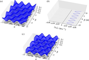
) is responsible for the increase of the wave shape asymmetry over time. An example is shown in figure 1. Two harmonics of equal frequency but propagating in different directions create a spatially varying shear over the sea surface (figure 1
b). This shear tends to slow down the troughs relatively to the crests leading to an asymmetric wave shape that can be related to the first stage of the formation of the well-known horseshoe patterns (see figure 1
c). The front–back symmetry of the waves and the absence of slope skewness are nonetheless preserved.
Interaction of two harmonics of equal amplitudes (
 $A=0.08~\text{m}$
) and wavenumbers (
 $k=1.104~\text{rad}~\text{m}^{-1}$
) but different directions of propagation:
 $+$
and
 $-$
48.2° relative to direction
 ${\it\alpha}$
. (a) Sea surface elevation at
 $t=0$
. (b)
 ${\it\alpha}$
component of the Stokes drift velocity:
 $\langle \boldsymbol{r}_{2t}\rangle _{t}$
(
 ${\it\beta}$
component vanishes). Such component is independent of
 ${\it\alpha}$
. We can see a mean Stokes drift of about
 $3~\text{cm}~\text{s}^{-1}$
and its spatial variations leading to increasing crescent shape patterns. (c) Sea surface elevation after a long time period of 30 s. The surface has developed distorted wave fronts.

Shrira, Badulin & Kharif (Reference Shrira, Badulin and Kharif1996) and later Annenkov & Shrira (Reference Annenkov and Shrira1999) proposed a mathematical solution to explain the apparition and the persistence of the horseshoe pattern by quintet resonant interactions coupled with wind and dissipation and noted that waves developed front–back asymmetries. The two main characteristics of the horseshoe patterns are (a) a life time largely exceeding the associated wave period and (b) a persistent shape with front–back asymmetry.
For clarity, in the explanations below, the term ‘harmonic’ is used for a Lagrangian wave vector component and the term ‘wave’ is used for an Eulerian (surface) wave vector component. Even though cross-comparison of harmonic interactions and wave interactions is not an easy task, we can try to estimate which harmonics are involved in the development of such wave front deformations. Bi-harmonic interaction terms are present in both horizontal (
 $x_{2},y_{2}$
) and vertical (
 $z_{2}$
) second-order Lagrangian displacements. Therefore, simply using bi-harmonic Lagrangian interactions should a priori make it possible to obtain, at least partially, the interactions of a wave quartet in the Eulerian framework. Horseshoe patterns observed by Collard & Caulliez (Reference Collard and Caulliez1999) present peculiar features that can be compared with the model presented. Their experiment starts from an almost monochromatic wave with wavenumber
 $\boldsymbol{k}_{0}$
. The wave field later degenerates and gives rise to crescent-shape patterns. The spatiotemporal analysis of this experiment shows that a pair of harmonics
 $(\boldsymbol{k}_{1},\boldsymbol{k}_{2})$
are created so that:
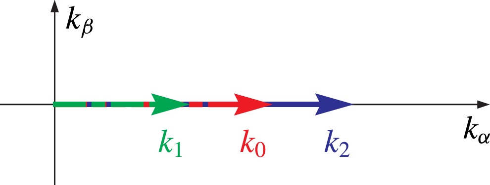
 $$\begin{eqnarray}\boldsymbol{k}_{1}+\boldsymbol{k}_{2}=3\boldsymbol{k}_{0}\quad \text{and}\quad {\it\omega}_{1}+{\it\omega}_{2}=3{\it\omega}_{0}.\end{eqnarray}$$
The case called ‘steady pattern’ in Collard & Caulliez (Reference Collard and Caulliez1999) is defined with
 $k_{1}=k_{2}$
and consequently
 ${\it\omega}_{1}={\it\omega}_{2}$
. In this specific case, the results presented in figure 1 suggest that no
 $\boldsymbol{k}_{0}$
component is necessary to obtain wave front deformation since the secular term in
 $\langle \boldsymbol{r}_{2t}\rangle _{t}-\langle \boldsymbol{r}_{2t}\rangle _{{\bf\xi}t}$
is generated by the
 $\boldsymbol{k}_{1}$
and
 $\boldsymbol{k}_{2}$
component interaction only. However, since the
 $\boldsymbol{k}_{0}$
component is obviously present in the experiment of Collard & Caulliez (Reference Collard and Caulliez1999), it was not experimentally possible to check whether such component is indispensable to the wave front deformation. Yet, it could be said that
 $\boldsymbol{k}_{0}$
is indirectly necessary to the emergence of the perfectly symmetric pair of wave vectors
 $(\boldsymbol{k}_{1},\boldsymbol{k}_{2})$
through the resonant interaction defined by (6.7). It should therefore be interesting to experimentally show that a unique bi-harmonic structure such as that presented in figure 1 is sufficient to create horseshoe patterns. However, in order to obtain such wave shapes, our methodology only performs satisfactorily when very low steepness and very long time periods are considered. Indeed, first- and second-order steady nonlinearities should remain low until the secular second-order term becomes observable. Experiments made by Kimmoun, Branger & Kharif (Reference Kimmoun, Branger and Kharif1999) show that beyond a certain level of steepness, no wave front asymmetry is observed and that steady first- and second-order nonlinearities, as described in § 6.3, become the main contributors to the wave shape deformation.
However, in the simulation presented in figure 1, the requirement of low steepness of the
 $\boldsymbol{k}_{1}$
and
 $\boldsymbol{k}_{2}$
component is fulfilled and, for comparison purposes with Collard & Caulliez (Reference Collard and Caulliez1999), we added a
 $\boldsymbol{k}_{0}$
component in the orbital spectrum which was chosen so that
 $\boldsymbol{k}_{1}+\boldsymbol{k}_{2}=3\boldsymbol{k}_{0}$
,
 ${\it\varphi}_{0}=-{\rm\pi}/2$
and
 ${\it\varphi}_{1}={\it\varphi}_{2}=0$
(but obviously where
 ${\it\omega}_{1}+{\it\omega}_{2}\neq 3{\it\omega}_{0}$
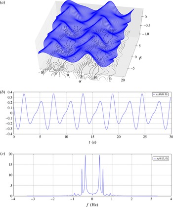
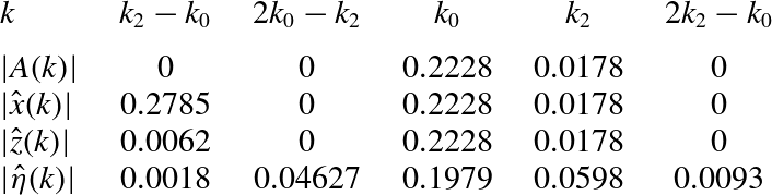
). This reproduced the ‘steady’ horseshoe patterns presented in Collard & Caulliez (Reference Collard and Caulliez1999). Figure 2(a) shows the wave field obtained after 30 s and figure 2(b,c) show the temporal record of the water surface elevation and its Fourier transform. As pointed out by Collard & Caulliez (Reference Collard and Caulliez1999), such wave field contains a
 $(3/2){\it\omega}_{0}$
harmonic (0.524 Hz) emanating from the simple first-order contribution of
 $\boldsymbol{k}_{1}$
and
 $\boldsymbol{k}_{2}$
. We believe that the front–back asymmetry of the horseshoe pattern observed in real conditions comes from higher-order interactions (Lagrangian cubic order) that would create a
 $\boldsymbol{k}_{0}$
component with an angular frequency of
 ${\it\omega}_{0}$
but with a slightly different phase.
Surface elevation obtained with three harmonics,
 $k_{0}=0.491~\text{rad}~\text{m}^{-1}$
,
 $k_{1}=k_{2}=1.104~\text{rad}~\text{m}^{-1}$
, respective amplitudes,
 $a_{0}=0.24~\text{m}$
and
 $a_{1}=a_{2}=0.06~\text{m}$
, directions of propagation relative to
 ${\it\alpha}$
,
 ${\it\theta}_{0}=0,{\it\theta}_{1}=-{\it\theta}_{2}=\arccos (2/3)$
, and phases
 ${\it\varphi}_{0}=-{\rm\pi}/2,{\it\varphi}_{1}={\it\varphi}_{2}=0$
. (a) Sea surface elevation at
 $t=30~\text{s}$
. (b) Temporal record of the water surface elevation at fixed point
 $({\it\alpha},{\it\beta})=(0,0)$
. (c) Fourier transform of the temporal record (figure 2
b). We can identify frequency
 $f_{0}=(2{\rm\pi})^{-1}\sqrt{gk_{0}}$
and harmonic
 $(3/2)f_{0}$
coming for
 $\boldsymbol{k}_{1}$
and
 $\boldsymbol{k}_{2}$
contribution.

In any case, even if the spatial drift we found tended to slowly twist the wave shape and made it tend towards the horseshoe pattern, this drift led to a constant increase of the surface deformation over time giving rise to unrealistic shapes after a long time period. Moreover, as already noted by Shrira et al. (Reference Shrira, Badulin and Kharif1996), steady wave solutions of inviscid equations do not present front–back asymmetries. Hence, the secular term can only belong to a transitory state of the surface and cannot be used for long time periods as suggested by the domain of validity of the series expansion.
As already mentioned, the Stokes drift manifests itself through a secular term which is undesirable in a perturbation expansion. Indeed, as commented by Buldakov et al. (Reference Buldakov, Taylor and Taylor2006), third-order solutions will make the secular term interact with the leading order creating unrealistic diverging secular terms in both horizontal and vertical particles expansion. As a result, the second-order solution cannot be valid at arbitrary long time periods. Furthermore, any attempt to pursue the Lagrangian expansion beyond the second order should be accompanied with a particles relabelling as suggested by Clamond (Reference Clamond2007) who claimed that a steady solution with Stokes drift cannot be found without adapting the Lagrangian references. The apparition of the mean secular term in a Lagrangian expansion comes from a misrepresentation of steady waves and can be avoided, at least in the case of a monochromatic wave, by a correct time-and-space-dependent water particles relabelling leading to a valid solution at all time and orders. However, as this paper deals with tri-dimensional multiple wave system and is restricted to the second-order expansion, we shall not enter into such details and leave these considerations for further studies.
6.3. Sharp crests, mean elevation and skewness coefficient
For the temporal mean of the second-order vertical displacement at the surface we write
 $$\begin{eqnarray}\langle z_{2}\rangle _{t,{\it\delta}=0}=\iint _{\mathbb{R}^{4}}{\eth}({\it\omega}-{\it\omega}^{\prime })\frac{1}{2}k\underline{{\mathcal{B}}}+\text{c.c.}\end{eqnarray}$$
This shows that the second-order vertical displacement has a non-vanishing mean due to the interaction of waves of equal frequency. The
 $(\widehat{\boldsymbol{k}}-\widehat{\boldsymbol{k}}^{\prime })$
phase term in
 $\underline{{\mathcal{B}}}$
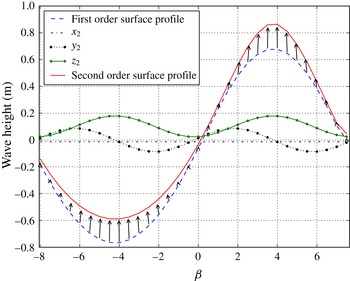
describes a spatial oscillating pattern perpendicular to the mean direction of the waves and is the main contributor to the vertical second-order displacement. To illustrate this statement, we use the same bi-harmonic system as described above. Figure 3 displays first- and second-order surface slices along an equi-
 ${\it\alpha}$
contour corresponding to a crest position. As can be plainly seen, the second-order vertical term tends to permanently sharpen the crests and flatten the troughs by a positive vertical shift relative to the
 $z_{2}$
mean level. Contrarily to the Lagrangian first-order terms, the sharpening and flattening effects apply in a direction perpendicular to the wave direction leading to a more ‘short-crested’ wave pattern. The horizontal term
 $y_{2}$
has the same effect even though it is in quadrature with the vertical motion. The combination of both effects is represented using arrows on figure 3.
Slices along an equi-
 ${\it\alpha}$
contour (perpendicular to the mean direction of wave) of the first- and second-order Lagrangian surface. The slices pass through a wave crest. The different second-order contributions are superimposed as well as their combined effects (arrows).

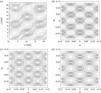
Kimmoun et al. (Reference Kimmoun, Branger and Kharif1999) used an advanced methodology to derive the surface topography from wave tank experiments. In their sixth experiments, two waves with equal wavelength and different directions interact and develop a short-crested wave field that is analysed and compared with their theoretical calculations. The second wave is obtained by reflexion of the first on a vertical wall. They pushed their theoretical Eulerian calculations up to the third order in the wave steepness parameter to compare with their observations. The sixth experiment (see figure 4 a) clearly shows ‘rhombic form of the crest and the elliptic form of the troughs’ that also appear on the second-order Lagrangian simulation plotted on figure 4(b). First-order Eulerian and Lagrangian simulations are respectively plotted in figure 4(c,d).
Interaction of two harmonics of equal amplitudes (
 $A=0.43~\text{cm}$
) and wavelength (
 ${\it\lambda}=7.8~\text{cm}$
) but different directions of propagation:
 $+$
and
 $-$
33° relative to direction
 ${\it\beta}$
: (a) figure 14 from Kimmoun et al. (Reference Kimmoun, Branger and Kharif1999); (b) second-order Lagrangian profile; (c) first-order Eulerian profile; (d) first-order Lagrangian profile.

It was shown by Pierson (Reference Pierson1961, equation (45)) that the first-order Lagrangian surface has a relative mean level:
 $$\begin{eqnarray}\overline{{\it\eta}}_{1}=-\int k\Vert A(\boldsymbol{k})\Vert ^{2}.\end{eqnarray}$$
The mean sea level is affected by the non-vanishing mean of the second-order elevation term (see mean level of
 $z_{2}$
on figure 3). At the surface,
 $$\begin{eqnarray}\langle z_{2}\rangle _{{\bf\xi},t}=\int \frac{1}{2}k\Vert A(\boldsymbol{k})\Vert ^{2}\end{eqnarray}$$
is the unique second-order contributor to mean surface elevation at the leading order giving the overall sea level:
 $$\begin{eqnarray}\overline{{\it\eta}}_{2}=-\int \frac{1}{2}k\Vert A(\boldsymbol{k})\Vert ^{2}.\end{eqnarray}$$
When this mean level is naturally tared by a Lagrangian sensor (free-floating buoys, etc.), it results in a mean sea level greater by an amount of
 $|\overline{{\it\eta}}_{2}|$
than an Eulerian measuring system (fixed probes, etc.) does. This conclusion has already been reached by Longuet-Higgins (Reference Longuet-Higgins1986) (see equation (3.7)) via a different route. The author emphasized the importance of this effect in particular with respect to ocean surface remote sensing applications. However, as already stated by Longuet-Higgins (Reference Longuet-Higgins1987), Lagrangian orbits are highly symmetrical at the second-order leading to a vanishing skewness. In random ocean wave fields, such second-order dynamical effects have strong impacts on waves height, slope and curvature distributions and are responsible for their deviation from the Gaussian law. These statistical properties are of great interest in the ocean remote-sensing community but a systematic study goes beyond the scope of this paper and is left for further developments.
6.4. Modulational Benjamin–Feir instability, a simple beat effect
It is now well known that Benjamin–Feir (BF) instability results from a nonlinear quartet-wave resonant phenomenon (Benjamin & Feir Reference Benjamin and Feir1967). An initial uniform monochromatic Stokes wave of moderate amplitude develops side-band harmonics with an exponential rate of growth and degenerates into a sequence of wave packets.
In this section we do not wish to enter into a complex analytical analysis but would like to show, on the basis of theoretical and numerical considerations, that the periodic regime of BF instability is already present (at least partly) and symmetric (i.e. with no frequency downshift) in the Lagrangian second-order solution.
We shall not study the growth period since we only consider periodic solutions but we shall show that, at the second order of the nonlinear Lagrangian parameter, a periodic modulation process exists between the carrier and two existing sideband harmonics and can be interpreted as a Lagrangian Benjamin–Feir modulation. We shall show that, surprisingly, what is considered to be a periodical exchange of energy between waves from a Eulerian point of view is in fact a simple beat effect which appears naturally when a two-wave system has close frequencies in the Lagrangian framework. The same initial sea state is used in the Eulerian framework and shows that this phenomenon is clearly absent up to the second order.
6.4.1. System of three aligned harmonics
In order to illustrate this statement, let us consider a bi-dimensional and unidirectional case defined up to the second order by (5.16) and (5.17). We focus on a bi-harmonics system defined by its wavenumbers
 $k_{0}$
and
 $k_{2}~(0<k_{0}<k_{2})$
where
 $k_{0}$
is the carrier wavenumber,
 $k_{2}$
the satellite wavenumber and
 ${\it\varphi}_{0}$
and
 ${\it\varphi}_{2}$
their respective phases. The carrier wave is chosen with wavenumber
 $k_{0}={\rm\pi}/2~\text{rad}~\text{m}^{-1}$
propagating in the
 ${\it\alpha}$
direction and corresponding to a 4 m wavelength and a 1.6 s time period. Its orbital amplitude
 $a_{0}=0.2228~\text{m}$
is chosen so that
 $s=k_{0}a_{0}=0.35$
. It must however be emphasized that
 $a_{0}$
is the orbital spectral amplitude and that the real amplitude of the carrier never exceed 0.2 m leading to a maximum steepness of 0.3. The satellite wavenumber is
 $k_{2}=k_{0}\times (1+p)$
with
 $p=0.1$
. Its orbital amplitude is
 $a_{2}=a_{0}\times c$
with
 $c=0.08$
.
We generate a surface of 90 m length with a 12.5 cm label spatial sampling over a thousand periods of the carrier wave and evaluate, at each step in time, the spectral amplitude of the surface
 ${\it\eta}({\it\alpha},t)$
(a numerical interpolation of the surface profile on a regular grid was realized prior to its Fourier transform), the horizontal
 $x({\it\alpha},t)$
and vertical
 $z({\it\alpha},t)$
particle displacement processes at the surface
 ${\it\delta}=0$
. We therefore evaluate the Fourier transforms
 $\hat{{\it\eta}}(k,t)$
,
 $\hat{x}(k,t)$
and
 $\hat{z}(k,t)$
defined by
 $$\begin{eqnarray}\hat{{\it\Psi}}(k,t)=\int ({\it\Psi}({\it\alpha},t)-\overline{{\it\Psi}})\text{e}^{\text{i}k{\it\alpha}}\,\text{d}{\it\alpha},\end{eqnarray}$$
where
 ${\it\Psi}$
stands for any of the three quantities
 ${\it\eta}$
,
 $x$
or
 $z$
and where the upper line
 $\overline{{\it\Psi}}$
refers to the spatial average. These quantities are constant in time and are given in table 1 together with the orbital spectral amplitudes
 $|A(k)|$
. We have selected the wavenumbers associated to non-vanishing amplitudes. All harmonics of the orbital spectrum are aligned and produce a unique temporal secular term corresponding to a global horizontal translation of the sea surface profile. This main constant drift can easily be removed by adapting the frame of reference ensuring the validity of the second-order expansion, in this case only, even for long time periods.
Orbital
 $|A(k)|$
, horizontal
 $|\hat{x}|$
, vertical
 $|\hat{z}|$
motions and surface
 $|\hat{{\it\eta}}|$
spectral amplitudes obtained from a two-wave orbital system:
 $(k_{0},k_{2})={\rm\pi}/2\times (1,1+p)$
and
 $(a_{0},a_{2})=s/k_{0}\times (1,c)$
with
 $s=0.35$
,
 $p=0.1$
and
 $c=0.08$
.

Even though neither the vertical
 $|\hat{z}|$
nor horizontal
 $|\hat{x}|$
displacement spectra contain a
 $2k_{0}-k_{2}$
component, this component is present in the surface spectrum. The
 $k_{2}-k_{0}$
component is an important contributor to the second-order horizontal displacement:
 $$\begin{eqnarray}-\!{\displaystyle \frac{a_{0}a_{2}}{g}}\left({\displaystyle \frac{{\it\omega}_{0}^{3}+{\it\omega}_{2}^{3}}{{\it\omega}_{2}-{\it\omega}_{0}}}\right)\sin \left[(k_{2}-k_{0})x-({\it\omega}_{2}-{\it\omega}_{0})t+{\it\varphi}_{2}-{\it\varphi}_{0}\right].\end{eqnarray}$$
Table 1 clearly shows the
 $k_{0}-(k_{2}-k_{0})=2k_{0}-k_{2}$
harmonic in the surface spectrum due to the combination of the horizontal
 $k_{2}-k_{0}$
term and the
 $k_{0}$
term. We can therefore easily deduce that the angular frequency and phase of this term become
 $2{\it\omega}_{0}-{\it\omega}_{2}$
and
 $2{\it\varphi}_{0}-{\it\varphi}_{2}$
. The other interaction term with wavenumber
 $k_{0}+(k_{2}-k_{0})=k_{2}$
has the same frequency
 ${\it\omega}_{2}$
and phase
 ${\it\varphi}_{2}$
as the orbital first-order
 $k_{2}$
component of the orbital spectrum and simply affects its amplitude.
The case presented in table 1 shows that the
 $k_{2}$
component of the surface spectrum benefits from a constructive interaction of the
 $k_{0}$
and
 $(k_{2}-k_{0})$
terms since its amplitude (0.0598) is increased relatively to the specified orbital amplitude (0.0178). Conversely, the amplitude of the
 $k_{0}$
component is decreased relatively to orbital amplitude due to a destructive interaction. As expected, the surface spectrum also contains a very small
 $2k_{2}-k_{0}$
term arising from the combination term
 $k_{2}+(k_{2}-k_{0})$
.
Now, let us suppose that an extra
 $k_{1}$
component is added to the orbital spectrum in such a way that
 $k_{1}=2k_{0}-k_{2}$
as shown in figure 5 and denote
 ${\it\omega}_{1}$
and
 ${\it\varphi}_{1}$
as the associated angular frequency and phase. This component will therefore have the same spatial wavenumber as the
 $k_{0}-(k_{2}-k_{0})$
term presented above but with a slightly different temporal frequency. These two terms will therefore generate a temporal beat effect with angular frequency
 ${\rm\Delta}{\it\omega}$
such as
 $$\begin{eqnarray}{\rm\Delta}{\it\omega}={\it\omega}_{1}-(2{\it\omega}_{0}-{\it\omega}_{2})\end{eqnarray}$$
and thus the phase of
 $k_{1}$
amplitude temporal evolution will only depend on the global phase:
 $$\begin{eqnarray}{\it\theta}={\it\varphi}_{1}-(2{\it\varphi}_{0}-{\it\varphi}_{2}).\end{eqnarray}$$
Inverting
 $k_{1}$
and
 $k_{2}$
in the previous considerations we obtain the same behaviour for the
 $k_{2}$
component. Now, letting the triple-harmonic structure system evolve in time leads to a periodic evolution of the two side-band harmonic amplitudes which share the same time period:
 $$\begin{eqnarray}T={\displaystyle \frac{2{\rm\pi}}{{\rm\Delta}{\it\omega}}}\end{eqnarray}$$
and the same evolution phase depending on the unique value
 ${\it\theta}$
. The time evolution of the carrier, high-frequency (HF) and low-frequency (LF) side-band amplitudes is presented in figure 6. The corresponding Eulerian case is presented for comparison purposes and clearly shows that the BF modulation is absent up to the second order. Shemer (Reference Shemer2010) had already derived these two results using a different technique in the Eulerian framework by pushing the nonlinearity at the third order and considering the evolution of a wave quartet.
Spectral repartition of the orbital spectrum components with
 $k_{1}+k_{2}=2k_{0}$
.

Time evolution of the spectral amplitudes of the carrier wave (
 ${\it\omega}_{0}=3.93~\text{rad}~\text{s}^{-1}$
), the low- and the high-frequency sidebands (
 ${\it\omega}_{1}=3.74$
and
 ${\it\omega}_{2}=4.11~\text{rad}~\text{s}^{-1}$
). Solid lines represent the Lagrangian expansion and dashed lines the Eulerian expansion. The period defined in (6.16) is 726 s.

It should be noted that the mean level and the variations of each satellite amplitude are not fully controlled by the ratio
 $c=a_{2}/a_{0}$
and depend on the carrier characteristics and on the other satellite. This makes the quantitative comparison between the two approaches complicated. However, it does not change the conclusion that a strong modulation–demodulation of the carrier wave and of the two satellites is present at the second order in the Lagrangian framework while the Eulerian point of view does not show any interaction even if the sea surface spectrum presents new harmonics relative to the first order.
6.4.2. Carrier harmonic with two lateral side-band harmonics
Let us now consider a symmetric triple-harmonic structure such as
 $2\boldsymbol{k}_{0}=\boldsymbol{k}_{1}+\boldsymbol{k}_{2}$
with
 ${\it\omega}_{1}-{\it\omega}_{0}>0$
and
 ${\it\omega}_{2}-{\it\omega}_{0}>0$
. This configuration is possible in the tri-dimensional case only and is represented in figure 7. Figure 8 show surface profiles derived using second-order solutions of the Eulerian (Longuet-Higgins Reference Longuet-Higgins1963) expansion and the Lagrangian (2.7) expansion with (3.7) and (4.47) using the same triple-harmonic structure. The carrier wave is chosen with amplitude
 $a_{0}=0.2~\text{m}$
and propagates in the
 ${\it\alpha}$
direction with wavenumber
 $k_{0}=1.58~\text{rad}~\text{m}^{-1}$
corresponding to a 3.97 m wavelength and a 1.58 s time period. Two satellites of equal amplitude
 $a_{1}=a_{2}=0.04~\text{m}$
with wavenumbers
 $k_{1}=k_{2}=k_{0}/[\cos (37.08^{\circ })]~\text{rad}~\text{m}^{-1}$
propagate with angles
 $+37.08^{\circ }$
and
 $-37.08^{\circ }$
relative to the
 ${\it\alpha}$
direction. The phases of each of the three harmonics are set to zero. Spatial sampling is 25 cm.
Spectral repartition of the orbital spectrum components with
 $\boldsymbol{k}_{1}+\boldsymbol{k}_{2}=2\boldsymbol{k}_{0}$
.

Sea surface profiles derived from second-order solutions of Lagrangian (a) and Eulerian (b) expansion. Here
 $t=17~\text{s}$
.

We generate an
 $8~\text{m}\times 8~\text{m}$
surface with a 25 cm spatial sampling over 10 periods of the carrier wave and a time evolution process is realized by increasing the time variable. A bi-dimensional spectral analysis of the surfaces is realized at each step in time by fast Fourier transform. Again, a numerical interpolation of the Lagrangian surface on a regular grid is realized prior to the Fourier transform. Figure 9 shows the surfaces spectra obtained at
 $t=17~\text{s}$
showing the three-wave pattern. As expected, the surface in the Lagrangian framework contains more harmonics than in the Eulerian framework due to the multiple possible combinations between horizontal and vertical particle harmonics. Figure 10 shows the time evolution of the three harmonic amplitudes. Again, the Eulerian case is presented for comparison purposes showing that the BF modulation is absent.
Eulerian (a) and Lagrangian (b) surface spectra. Here
 $t=17~\text{s}$
.

Evolution of the carrier and satellites amplitudes as a function of time.

In the presented tri-dimensional structure, we can see that sideband harmonics modulations are synchronous leading to strong opposite modulation between carrier and harmonics amplitudes. We can also see that the mean amplitude of the carrier in the Lagrangian framework is always notably smaller than the prescribed value (0.2) which is the consequence of constructive harmonics interactions. This decrease of the carrier amplitude is amplified by the fact that the prescribed amplitude is the orbital spectrum amplitude and not the sea surface spectrum amplitude. On the contrary, the two sideband harmonics take advantage of the positive interaction permanently increasing their mean amplitudes. In any case, the observed modulation depth is related to the amplitude of the second-order horizontal term relatively to the first-order component having the same wavenumber. Moreover, we note that the horizontal second-order term is inversely proportional to the difference of the carrier and sideband harmonic frequencies (see (6.13)). Increasing this difference rapidly leads to a strong reduction of the modulation process. Additional numerical simulations with greater frequency differences between the carrier and the sideband harmonics were made and confirm this statement, which is consistent with the proximity of the frequencies observed in BF instability experiments.
Here, we focus on the modulation–demodulation resonance that can be related to a BF modulational instability. We have shown that, from a Lagrangian point of view, no energy is exchanged between the involved orbital harmonics. Conversely, the Eulerian interpretation of this phenomenon, based on the surface spectrum analysis instead of the orbital analysis, is a permanent and periodical energy exchange between the carrier wave and its two sideband harmonics. This shows that the Lagrangian formulation is in a certain way a more natural and easier point of view. Moreover, in the Lagrangian framework, the time invariability of the harmonics amplitudes suggests that the side-band generation process (the instability itself) can be clearly separated from the modulational part (beating phenomena). However, it is known that asymmetric evolution of the sideband harmonics, responsible for the frequency down-shift effect, is obtained when the modulation increases and when stronger nonlinear effects or dissipation are taken into account. These phenomena are clearly absent at the Lagrangian second-order and will be considered in future studies together with the derivation of the instability domain of an initial monochromatic Stokes wave.
7. Conclusion
In this paper, the second-order perturbation expansion in Lagrangian coordinates has been derived to study the interactions between deep-water surface gravity waves. In its compact and vectorial form, the proposed solution extends initial investigations (Pierson Reference Pierson1961), fully recovers the classical second-order Eulerian expansion (Longuet-Higgins Reference Longuet-Higgins1963) and naturally includes the well-known Stokes drift velocity. As further illustrated in the case of tri-dimensional wave interactions, a residual spatial Stokes drift will result from harmonics of equal frequency but having different propagation directions. This phenomenon leads to an increase of the wave shape asymmetry along the propagation, and can be related to the development of short-crested wave patterns, as a possible initial stage of formation of horseshoe patterns. Indeed, Lagrangian second-order terms will contribute to sharpening and flattening effects, but, contrary to the first-order correction, these effects are applied in the perpendicular direction to the wave’s direction.
The modulation aspect of the BF instability is further shown to be captured as a beat effect in the Lagrangian framework. A periodic modulation emerges between the carrier and two sideband harmonics. As demonstrated, the orbital spectrum remains unchanged as the waves evolve in time, while the corresponding surface Eulerian spectrum exhibits periodical variations for the carrier and sideband harmonic amplitudes. It should be noted that the asymmetric evolution of the sideband harmonics, and the associated frequency downshift, are not recovered at this second Lagrangian order.
The extension of the proposed expansion to the case of varying depth and surface current could also follow the same formalism, and its further investigation should be considered in the future.
Acknowledgements
F.N. would like to thank the Centre National de la Recherche Scientifique (CNRS) and Université de Toulon (chaire mixte) for their support. Part of this work was done during a long-term visit to the Laboratoire d’Oceanographie Spatiale, IFREMER Brest.
Appendix A
A.1. Perfect differential and vorticity
There is no vorticity if the velocity field
 $\boldsymbol{R}_{t}$
can be written in the form:
 $$\begin{eqnarray}\boldsymbol{R}_{t}=\boldsymbol{{\rm\nabla}}F\end{eqnarray}$$
where
 $F$
is any scalar function. Noting that
 $\text{d}F=\boldsymbol{{\rm\nabla}}F\boldsymbol{\cdot }\text{d}\boldsymbol{R}$
, we thus have
 $$\begin{eqnarray}\text{d}F=x_{t}\,\text{d}x+y_{t}\,\text{d}y+z_{t}\,\text{d}z.\end{eqnarray}$$
Replacing terms
 $\text{d}x,\text{d}y$
and
 $\text{d}z$
by their respective particle-label-dependent expressions:
 $$\begin{eqnarray}\displaystyle & \text{d}x=x_{{\it\alpha}}\,\text{d}{\it\alpha}+x_{{\it\beta}}\,\text{d}{\it\beta}+x_{{\it\delta}}\,\text{d}{\it\delta} & \displaystyle\end{eqnarray}$$
 $$\begin{eqnarray}\displaystyle & \text{d}y=y_{{\it\alpha}}\,\text{d}{\it\alpha}+y_{{\it\beta}}\,\text{d}{\it\beta}+y_{{\it\delta}}\,\text{d}{\it\delta} & \displaystyle\end{eqnarray}$$
 $$\begin{eqnarray}\displaystyle & \text{d}z=z_{{\it\alpha}}\,\text{d}{\it\alpha}+z_{{\it\beta}}\,\text{d}{\it\beta}+z_{{\it\delta}}\,\text{d}{\it\delta} & \displaystyle\end{eqnarray}$$
 $\text{d}{\bf\zeta}=(\text{d}{\it\alpha},\text{d}{\it\beta},\text{d}{\it\delta})$
denotes an infinitesimal label variation, we can rewrite
 $$\begin{eqnarray}\text{d}F=(\mathbb{J}\boldsymbol{R}_{t})\boldsymbol{\cdot }\text{d}{\bf\zeta}\end{eqnarray}$$
where
 $\mathbb{J}$
is defined in (2.4). Thereby, if a function
 $F({\bf\zeta},t)$
can be found such that
 $\text{d}F$
is a perfect differential, there is no vorticity.
A.2. Combination of first-order terms in Newton’s law
Consider the right-hand side of (4.1),
 $-\unicode[STIX]{x1D643}({\it\Phi}_{1})\boldsymbol{{\rm\nabla}}{\it\Phi}_{1tt}$
, where
 $\unicode[STIX]{x1D643}$
and
 $\boldsymbol{{\rm\nabla}}$
are respectively the Hessian and the gradient operator:
 $$\begin{eqnarray}\unicode[STIX]{x1D643}({\it\Phi}_{1})=\left[\begin{array}{@{}ccc@{}}{\it\phi}_{1{\it\alpha}{\it\alpha}} & {\it\phi}_{1{\it\alpha}{\it\beta}} & {\it\phi}_{1{\it\alpha}{\it\delta}}\\ {\it\phi}_{1{\it\alpha}{\it\beta}} & {\it\phi}_{1{\it\beta}{\it\beta}} & {\it\phi}_{1{\it\beta}{\it\delta}}\\ {\it\phi}_{1{\it\alpha}{\it\delta}} & {\it\phi}_{1{\it\beta}{\it\delta}} & {\it\phi}_{1{\it\delta}{\it\delta}}\end{array}\right]+\text{c.c.}\quad \text{and}\quad \boldsymbol{{\rm\nabla}}{\it\Phi}_{1tt}=\left[\begin{array}{@{}c@{}}{\it\phi}_{1{\it\alpha}tt}\\ {\it\phi}_{1{\it\beta}tt}\\ {\it\phi}_{1{\it\delta}tt}\end{array}\right]+\text{c.c.}\end{eqnarray}$$
We can write
 $-\unicode[STIX]{x1D643}({\it\Phi}_{1})\boldsymbol{{\rm\nabla}}{\it\Phi}_{1tt}=\boldsymbol{S}+\boldsymbol{T}$
where
 $\boldsymbol{S}=(S^{{\it\alpha}},S^{{\it\beta}},S^{{\it\delta}})$
and
 $\boldsymbol{T}=(T^{{\it\alpha}},T^{{\it\beta}},T^{{\it\delta}})$
are tri-dimensional vectors:
 $$\begin{eqnarray}\displaystyle \boldsymbol{S}=-\unicode[STIX]{x1D643}({\it\phi}_{1})\boldsymbol{{\rm\nabla}}{\it\phi}_{1tt}+\text{c.c.} & & \displaystyle\end{eqnarray}$$
 $$\begin{eqnarray}\displaystyle \boldsymbol{T}=-\unicode[STIX]{x1D643}({\it\phi}_{1})\boldsymbol{{\rm\nabla}}{\it\phi}_{1tt}^{\ast }+\text{c.c.} & & \displaystyle\end{eqnarray}$$
 $\text{}^{\ast }$
’ means the complex conjugate. We will investigate successively the explicit form of
 $\boldsymbol{S}$
and
 $\boldsymbol{T}$
. Introducing the two kernels
 $$\begin{eqnarray}\displaystyle & {\mathcal{K}}={\displaystyle \frac{1}{4}}{\displaystyle \frac{A(\boldsymbol{k})A(\boldsymbol{k}^{\prime })}{kk^{\prime }}}\text{e}^{\text{i}(\boldsymbol{k}+\boldsymbol{k}^{\prime })\boldsymbol{\cdot }{\bf\xi}-\text{i}({\it\omega}+{\it\omega}^{\prime })t}\text{e}^{(k+k^{\prime }){\it\delta}} & \displaystyle\end{eqnarray}$$
 $$\begin{eqnarray}\displaystyle & \underline{{\mathcal{K}}}={\displaystyle \frac{1}{4}}{\displaystyle \frac{A(\boldsymbol{k})A^{\ast }(\boldsymbol{k}^{\prime })}{kk^{\prime }}}\text{e}^{\text{i}(\boldsymbol{k}-\boldsymbol{k}^{\prime })\boldsymbol{\cdot }{\bf\xi}-\text{i}({\it\omega}-{\it\omega}^{\prime })t}\text{e}^{(k+k^{\prime }){\it\delta}} & \displaystyle\end{eqnarray}$$
 ${\it\phi}_{1}$
expression, the
 ${\it\alpha}$
component of
 $\boldsymbol{S}$
can be written
 $$\begin{eqnarray}\displaystyle S^{{\it\alpha}}\! & = & \displaystyle \!-\iint \left[(\text{i}k_{{\it\alpha}})^{2}(\text{i}k_{{\it\alpha}}^{\prime })(-\text{i}{\it\omega}^{\prime })^{2}+(\text{i}k_{{\it\alpha}})(\text{i}k_{{\it\beta}})(\text{i}k_{{\it\beta}}^{\prime })(-\text{i}{\it\omega}^{\prime })^{2}+(\text{i}k_{{\it\alpha}})kk^{\prime }(-\text{i}{\it\omega}^{\prime })^{2}\right]{\mathcal{K}}+\text{c.c.}\nonumber\\ \displaystyle & = & \displaystyle \!-\iint \text{i}k_{{\it\alpha}}gk^{\prime }\left[k_{{\it\alpha}}k_{{\it\alpha}}^{\prime }+k_{{\it\beta}}k_{{\it\beta}}^{\prime }-kk^{\prime }\right]{\mathcal{K}}+\text{c.c.}\nonumber\\ \displaystyle & = & \displaystyle \!\iint \text{i}k_{{\it\alpha}}gk^{\prime }(kk^{\prime }-\boldsymbol{k}\boldsymbol{\cdot }\boldsymbol{k}^{\prime }){\mathcal{K}}+\text{c.c.}\end{eqnarray}$$
Making use of the symmetric integration over
 $k$
and
 $k^{\prime }$
in the second term we can rewrite
 $$\begin{eqnarray}S^{{\it\alpha}}=\iint g{\displaystyle \frac{\text{i}kk^{\prime }}{2}}\left({\displaystyle \frac{k_{{\it\alpha}}}{k}}+{\displaystyle \frac{k_{{\it\alpha}}^{\prime }}{k^{\prime }}}\right)(kk^{\prime }-\boldsymbol{k}\boldsymbol{\cdot }\boldsymbol{k}^{\prime }){\mathcal{K}}+\text{c.c.}\end{eqnarray}$$
The same procedure can be applied to the
 ${\it\beta}$
component, leading to
 $$\begin{eqnarray}(S^{{\it\alpha}},S^{{\it\beta}})=\iint {\mathcal{N}}gkk^{\prime }{\displaystyle \frac{\text{i}(\widehat{\boldsymbol{k}}+\widehat{\boldsymbol{k}^{\prime }})}{2}}+\text{c.c.}\end{eqnarray}$$
where
 ${\mathcal{N}}$
is defined is (4.8). As to the
 ${\it\delta}$
component of
 $\boldsymbol{S}$
, it is found to be
 $$\begin{eqnarray}\displaystyle S^{{\it\delta}} & = & \displaystyle -\iint \left[(\text{i}k_{{\it\alpha}})k(\text{i}k_{{\it\alpha}}^{\prime })(-\text{i}{\it\omega}^{\prime })^{2}+(\text{i}k_{{\it\beta}})k(\text{i}k_{{\it\beta}}^{\prime })(-\text{i}{\it\omega}^{\prime })^{2}+k^{2}k^{\prime }(-\text{i}{\it\omega}^{\prime })^{2}\right]{\mathcal{K}}+\text{c.c.}\nonumber\\ \displaystyle & = & \displaystyle \iint {\mathcal{N}}gkk^{\prime }+\text{c.c.}\end{eqnarray}$$
For the
 ${\it\alpha}$
component of
 $\boldsymbol{T}$
,
 $$\begin{eqnarray}T^{{\it\alpha}}=\iint \text{i}k_{{\it\alpha}}gk^{\prime }(\boldsymbol{k}\boldsymbol{\cdot }\boldsymbol{k}^{\prime }+kk^{\prime })\underline{{\mathcal{K}}}+\text{c.c.},\end{eqnarray}$$
we invert
 $\boldsymbol{k}$
and
 $\boldsymbol{k}^{\prime }$
in the c.c. expression to obtain
 $$\begin{eqnarray}T^{{\it\alpha}}=\iint g{\displaystyle \frac{\text{i}kk^{\prime }}{2}}\left({\displaystyle \frac{k_{{\it\alpha}}}{k}}-{\displaystyle \frac{k_{{\it\alpha}}^{\prime }}{k^{\prime }}}\right)(kk^{\prime }+\boldsymbol{k}\boldsymbol{\cdot }\boldsymbol{k}^{\prime })\underline{{\mathcal{K}}}+\text{c.c.}\end{eqnarray}$$
Applying the same technique to the
 ${\it\beta}$
component we come up with (4.6) which can be written
 $$\begin{eqnarray}\displaystyle (T^{{\it\alpha}},T^{{\it\beta}}) & = & \displaystyle \iint {\displaystyle \frac{\text{i}(\widehat{\boldsymbol{k}}-\widehat{\boldsymbol{k}^{\prime }})}{2}}gkk^{\prime }(\boldsymbol{k}\boldsymbol{\cdot }\boldsymbol{k}^{\prime }+kk^{\prime })\underline{{\mathcal{K}}}+\text{c.c.}\end{eqnarray}$$
 $$\begin{eqnarray}\displaystyle & = & \displaystyle \iint {\displaystyle \frac{\text{i}(\widehat{\boldsymbol{k}}-\widehat{\boldsymbol{k}^{\prime }})}{2}}gkk^{\prime }\underline{{\mathcal{N}}}+\text{c.c.}\end{eqnarray}$$
 ${\it\delta}$
component of
 $\boldsymbol{T}$
can easily be derived as
 $$\begin{eqnarray}\displaystyle T^{{\it\delta}} & = & \displaystyle \iint gkk^{\prime }(kk^{\prime }+\boldsymbol{k}\boldsymbol{\cdot }\boldsymbol{k}^{\prime })\underline{{\mathcal{K}}}+\text{c.c.}\end{eqnarray}$$
 $$\begin{eqnarray}\displaystyle & = & \displaystyle \iint gkk^{\prime }\underline{{\mathcal{N}}}+\text{c.c.}\end{eqnarray}$$
A.3. Combination of first-order terms in the conservation law
The combination of first-order terms in the conservation law (4.12) can be written
 $$\begin{eqnarray}{\it\Phi}_{1{\it\alpha}{\it\alpha}}{\it\Phi}_{1{\it\beta}{\it\beta}}+{\it\Phi}_{1{\it\alpha}{\it\alpha}}{\it\Phi}_{1{\it\delta}{\it\delta}}+{\it\Phi}_{1{\it\beta}{\it\beta}}{\it\Phi}_{1{\it\delta}{\it\delta}}-{\it\Phi}_{1{\it\alpha}{\it\beta}}^{2}-{\it\Phi}_{1{\it\alpha}{\it\delta}}^{2}-{\it\Phi}_{1{\it\beta}{\it\delta}}^{2}\end{eqnarray}$$
where
 ${\it\Phi}_{1}={\it\phi}_{1}+{\it\phi}_{1}^{\ast }$
. After the combination of all of the terms in the form
 ${\it\phi}_{1mn}{\it\phi}_{1pq}$
and
 ${\it\phi}_{1mn}^{\ast }{\it\phi}_{1pq}^{\ast }$
where
 $m,n,p,q$
can be any of the variables
 ${\it\alpha},~{\it\beta}$
or
 ${\it\delta}$
we obtain
 $$\begin{eqnarray}\displaystyle & & \displaystyle \iint \left[(\text{i}k_{{\it\alpha}})^{2}(\text{i}k_{{\it\beta}}^{\prime })^{2}+(\text{i}k_{{\it\alpha}})^{2}k^{\prime 2}+(\text{i}k_{{\it\beta}})^{2}k^{\prime 2}-(\text{i}k_{{\it\alpha}})(\text{i}k_{{\it\beta}})(\text{i}k_{{\it\alpha}}^{\prime })(\text{i}k_{{\it\beta}}^{\prime })\right.\nonumber\\ \displaystyle & & \displaystyle \qquad \left.-\,(\text{i}k_{{\it\alpha}})k(\text{i}k_{{\it\alpha}}^{\prime })k^{\prime }-(\text{i}k_{{\it\beta}})k(\text{i}k_{{\it\beta}}^{\prime })k^{\prime }\right]{\mathcal{K}}+\text{c.c.}\nonumber\\ \displaystyle & & \displaystyle \quad =\iint \left[\frac{1}{2}(k_{{\it\alpha}}k_{{\it\beta}}^{\prime }-k_{{\it\beta}}k_{{\it\alpha}}^{\prime })^{2}+kk^{\prime }(\boldsymbol{k}\boldsymbol{\cdot }\boldsymbol{k}^{\prime }-kk^{\prime })\right]{\mathcal{K}}+\text{c.c.}\nonumber\\ \displaystyle & & \displaystyle \quad =-\iint \left[kk^{\prime }(1-\widehat{\boldsymbol{k}}\boldsymbol{\cdot }\widehat{\boldsymbol{k}}^{\prime }){\displaystyle \frac{kk^{\prime }-\boldsymbol{k}\boldsymbol{\cdot }\boldsymbol{k}^{\prime }}{2}}\right]{\mathcal{K}}+\text{c.c.}\nonumber\\ \displaystyle & & \displaystyle \quad =-\iint {\displaystyle \frac{kk^{\prime }-\boldsymbol{k}\boldsymbol{\cdot }\boldsymbol{k}^{\prime }}{2}}{\mathcal{N}}+\text{c.c.}\end{eqnarray}$$
In the same manner, the combination of the terms
 ${\it\phi}_{1mn}{\it\phi}_{1pq}^{\ast }$
gives
 $$\begin{eqnarray}-\iint {\displaystyle \frac{kk^{\prime }+\boldsymbol{k}\boldsymbol{\cdot }\boldsymbol{k}^{\prime }}{2}}\underline{{\mathcal{N}}}+\text{c.c.}\end{eqnarray}$$
Appendix B
In this appendix we prove the existence of the following integral in the sense of the Cauchy PV:
 $$\begin{eqnarray}\underline{\boldsymbol{r}}_{2}=\text{PV}\iint _{\mathbb{R}^{4}}\text{i}{\displaystyle \frac{{\it\omega}\boldsymbol{k}+{\it\omega}^{\prime }\boldsymbol{k}^{\prime }}{2({\it\omega}-{\it\omega}^{\prime })}}\underline{{\mathcal{B}}}\text{e}^{-\text{i}({\it\omega}-{\it\omega}^{\prime })t}\text{e}^{(k+k^{\prime }){\it\delta}}+\text{c.c.}\end{eqnarray}$$
By definition, this can be rewritten
 $$\begin{eqnarray}\underline{\boldsymbol{r}}_{2}=\lim _{{\it\gamma}\rightarrow 0}\iint _{\mathbb{R}^{4}-{\mathcal{E}}}-{\displaystyle \frac{\unicode[STIX]{x1D643}(\boldsymbol{k},\boldsymbol{k}^{\prime })}{4({\it\omega}-{\it\omega}^{\prime })}}\text{e}^{(k+k^{\prime }){\it\delta}}\end{eqnarray}$$
where
 ${\mathcal{E}}$
is the domain such as
 $|{\it\omega}-{\it\omega}^{\prime }|<{\it\gamma}$
and
 $$\begin{eqnarray}\unicode[STIX]{x1D643}(\boldsymbol{k},\boldsymbol{k}^{\prime })=({\it\omega}\boldsymbol{k}+{\it\omega}^{\prime }\boldsymbol{k}^{\prime })(1+\widehat{\boldsymbol{k}}\boldsymbol{\cdot }\widehat{\boldsymbol{k}}^{\prime })|A(\boldsymbol{k})||A(\boldsymbol{k}^{\prime })|\sin [(\boldsymbol{k}-\boldsymbol{k}^{\prime })\boldsymbol{\cdot }{\bf\xi}-({\it\omega}-{\it\omega}^{\prime })t+{\it\varphi}_{\boldsymbol{ k}}-{\it\varphi}_{\boldsymbol{k}^{\prime }}]\end{eqnarray}$$
where
 ${\it\varphi}_{\boldsymbol{k}}$
and
 ${\it\varphi}_{\boldsymbol{k}^{\prime }}$
are respectively the phases of
 $A(\boldsymbol{k})$
and
 $A(\boldsymbol{k}^{\prime })$
. We denote
 $\unicode[STIX]{x1D643}^{0}(k,\widehat{\boldsymbol{k}},\widehat{\boldsymbol{k}}^{\prime })$
the value of (B 3) when
 $k=k^{\prime }~({\it\omega}={\it\omega}^{\prime })$
:
 $$\begin{eqnarray}\displaystyle \unicode[STIX]{x1D643}^{0}(k,\widehat{\boldsymbol{k}},\widehat{\boldsymbol{k}}^{\prime }) & = & \displaystyle \unicode[STIX]{x1D643}(\boldsymbol{k},k\widehat{\boldsymbol{k}}^{\prime })\nonumber\\ \displaystyle & = & \displaystyle {\it\omega}k(\widehat{\boldsymbol{k}}+\widehat{\boldsymbol{k}}^{\prime })(1+\widehat{\boldsymbol{k}}\boldsymbol{\cdot }\widehat{\boldsymbol{k}}^{\prime })|A(\boldsymbol{k})||A(k\widehat{\boldsymbol{k}}^{\prime })|\sin [k(\widehat{\boldsymbol{k}}-\widehat{\boldsymbol{k}}^{\prime })\boldsymbol{\cdot }{\bf\xi}+{\it\varphi}_{\boldsymbol{k}}-{\it\varphi}_{k\widehat{\boldsymbol{k}}^{\prime }}].\qquad\end{eqnarray}$$
Focusing now on the integral,
 $$\begin{eqnarray}\underline{\boldsymbol{r}}_{2}^{0}=\lim _{{\it\gamma}\rightarrow 0}\iint _{\mathbb{R}^{4}-{\mathcal{E}}}-{\displaystyle \frac{\unicode[STIX]{x1D643}^{0}(k,\widehat{\boldsymbol{k}},\widehat{\boldsymbol{k}}^{\prime })}{4({\it\omega}-{\it\omega}^{\prime })}}\text{e}^{(k+k^{\prime }){\it\delta}}\end{eqnarray}$$
and noting that
 $\unicode[STIX]{x1D643}^{0}(k,\widehat{\boldsymbol{k}}^{\prime },\widehat{\boldsymbol{k}})=-\unicode[STIX]{x1D643}^{0}(k,\widehat{\boldsymbol{k}},\widehat{\boldsymbol{k}}^{\prime })$
leads to a vanishing value of
 $\underline{\boldsymbol{r}}_{2}^{0}$
since integration is realized over all directions of
 $\boldsymbol{k}$
and
 $\boldsymbol{k}^{\prime }$
. We can thus rewrite (B 2) in the form
 $$\begin{eqnarray}\underline{\boldsymbol{r}}_{2}=\lim _{{\it\gamma}\rightarrow 0}\iint _{\mathbb{R}^{4}-{\mathcal{E}}}-{\displaystyle \frac{\unicode[STIX]{x1D643}(\boldsymbol{k},\boldsymbol{k}^{\prime })-\unicode[STIX]{x1D643}^{0}(k,\widehat{\boldsymbol{k}},\widehat{\boldsymbol{k}}^{\prime })}{4({\it\omega}-{\it\omega}^{\prime })}}\text{e}^{(k+k^{\prime }){\it\delta}}\end{eqnarray}$$
or, more explicitly,
 $$\begin{eqnarray}\displaystyle \underline{\boldsymbol{r}}_{2} & = & \displaystyle \lim _{{\it\gamma}\rightarrow 0}\iint _{\mathbb{R}^{4}-{\mathcal{E}}}\frac{\text{i}}{4}(1+\widehat{\boldsymbol{k}}\boldsymbol{\cdot }\widehat{\boldsymbol{k}}^{\prime })\text{e}^{(k+k^{\prime }){\it\delta}}\nonumber\\ \displaystyle & & \displaystyle \times \left[{\displaystyle \frac{({\it\omega}\boldsymbol{k}+{\it\omega}^{\prime }\boldsymbol{k}^{\prime })A(\boldsymbol{k})A^{\ast }(\boldsymbol{k}^{\prime })\text{e}^{\text{i}(\boldsymbol{k}-\boldsymbol{k}^{\prime })\boldsymbol{\cdot }{\bf\xi}-\text{i}({\it\omega}-{\it\omega}^{\prime })t}-k{\it\omega}(\widehat{\boldsymbol{k}}+\widehat{\boldsymbol{k}}^{\prime })A(\boldsymbol{k})A^{\ast }(k\widehat{\boldsymbol{k}}^{\prime })\text{e}^{\text{i}k(\widehat{\boldsymbol{k}}-\widehat{\boldsymbol{k}}^{\prime })\boldsymbol{\cdot }{\bf\xi}}}{{\it\omega}-{\it\omega}^{\prime }}}\right]\nonumber\\ \displaystyle & & \displaystyle +\,\text{c.c.}\end{eqnarray}$$
The limit when
 ${\it\omega}\rightarrow {\it\omega}^{\prime }$
of the term between brackets can be written
 $$\begin{eqnarray}-\!\text{i}k{\it\omega}(\widehat{\boldsymbol{k}}+\widehat{\boldsymbol{k}}^{\prime })A(\boldsymbol{k})A^{\ast }(k\widehat{\boldsymbol{k}}^{\prime })\text{e}^{\text{i}k(\widehat{\boldsymbol{k}}-\widehat{\boldsymbol{k}}^{\prime })\boldsymbol{\cdot }{\bf\xi}}t\end{eqnarray}$$
ensuring (B 2) to be a finite limit and that
 $\underline{\boldsymbol{r}}_{2}$
is integrable in the Cauchy PV sense.