







1. Introduction
Flow-induced vibration (FIV) of structures is an aero- or hydro-elastic phenomenon resulting from the complex coupled interaction between a fluid and a structure (often termed fluid–structure interaction – FSI). FIV poses a critical challenge in various engineering applications, such as the swaying of large structures like bridges and high-rise buildings in strong winds, where undesirable vibration can lead to structural failure or long-term fatigue. Conversely, FIV has been considered as a potential source of renewable energy to harness available kinetic energy from fluid flows (see Bernitsas et al. Reference Bernitsas, Raghavan, Ben-Simon and Garcia2008; Lee & Bernitsas Reference Lee and Bernitsas2011; Wang et al. Reference Wang, Du, Zhao and Sun2017; Soti et al. Reference Soti, Zhao, Thompson, Sheridan and Bhardwaj2018; Tamimi et al. Reference Tamimi, Armin, Shahvaghar-Asl, Naeeni and Zeinoddini2019; Lv et al. Reference Lv, Sun, Bernitsas and Sun2021; Lo et al. Reference Lo, Thompson, Hourigan and Zhao2024c). Therefore, this has motivated an increasing amount of research that aims to characterise, predict and control FIV (see Khalak & Williamson Reference Khalak and Williamson1996; Govardhan & Williamson Reference Govardhan and Williamson2000; Morse & Williamson Reference Morse and Williamson2009b; Wong et al. Reference Wong, Zhao, Lo Jacono, Thompson and Sheridan2017; Lo et al. Reference Lo, Thompson, Hourigan and Zhao2024a). Of interest in the present study, a machine-learning-based active control method is implemented to maximise the cross-flow FIV of a thin elliptical cylinder, which a recent study (Lo et al. Reference Lo, Hourigan, Thompson and Zhao2023) has shown to produce high amplitude oscillations.
The FIV response of an aeroelastic or elastically mounted bluff body can typically be characterised in terms of two distinct phenomena: vortex-induced vibration (VIV) and galloping. VIV occurs as a result of the periodic shedding of vortices, or at least shear layer vorticity variation (Menon & Mittal Reference Menon and Mittal2020), from an elastic or elastically mounted body leading to a periodic cross-flow forcing. VIV is self-limited due to the breakup of the symmetrically alternating von Kármán vortex street at large vibration amplitudes (Blevins Reference Blevins1990). Galloping, however, is caused by the asymmetric pressure distribution across the body arising from the changes in the instantaneous flow incidence angle as the body oscillates in the fluid. As both manifestations of FIV are dependent on the properties of the flow and the cylinder (e.g. flow velocity, Reynolds number, geometry, mass ratio, applied damping, structural stiffness), many past works have chosen parameters such that VIV and galloping occur separately and can be individually investigated (Brooks Reference Brooks1960). However, recent studies (see Nemes et al. Reference Nemes, Zhao, Jacono and Sheridan2012; Zhao, Hourigan & Thompson Reference Zhao, Hourigan and Thompson2018a) have shown that rich and complex fluid–structure interactions can also be observed when both FIV phenomena concurrently manifest in the dynamic response of an elastic or elastically mounted cylinder system.
One example of the co-manifestation of VIV and galloping relates to cylinders with elliptical geometries as parametrised by the elliptical ratio  $\varepsilon = b/a$, where
 $a$ and
 $b$ are the streamwise and cross-flow (transverse) dimensions, respectively. Since the circular cylinder is considered a special case of the elliptical geometry (with
 $\varepsilon = 1$) whose FIV response is VIV due to the inherent symmetry of the system (see the reviews of Bearman Reference Bearman1984; Williamson & Govardhan Reference Williamson and Govardhan2004), numerous studies have shown that the introduction of deformation, where
 $\varepsilon > 1$, causes the flow induced by a transversely oscillating elliptical cylinder to become more unstable (Hall Reference Hall1984; Navrose et al. Reference Navrose, Yogeswaran, Sen and Mittal2014; Zhao, Hourigan & Thompson Reference Zhao, Hourigan and Thompson2019; Vijay et al. Reference Vijay, Srinil, Zhu, Bao, Zhou and Han2020). However, it was only recently when Lo et al. (Reference Lo, Hourigan, Thompson and Zhao2023) investigated the effect of structural damping on the FIV dynamics of a thin
 $\varepsilon =5$ cylinder (see figure 1) that large-scale oscillation amplitudes, previously unseen for other geometries at similar
 ${U^*}$ values, were discovered. Coined the ‘hyper branch’, the nominal maximum amplitude of
 $A\approx 8b$ observed for this region was only limited by the width of the water-channel facility in which the experiments were conducted. Furthermore, the presence of a secondary vortex street (SVS) can be identified as the wake formed by the elliptical (airfoil-shaped) cylinder as it translates rapidly across the oncoming flow. It indicates that the approximately factor-of-five increase in maximum amplitude over the elliptical cylinder studies of Zhao et al. (Reference Zhao, Hourigan and Thompson2019) and Vijay et al. (Reference Vijay, Srinil, Zhu, Bao, Zhou and Han2020) can be attributed to the combined effect of VIV and a galloping-like movement-induced instability in the hyper-branch reduced-velocity range. Additionally, when a non-zero orientation angle
 $\theta$ is introduced for an
 $\varepsilon =5$ cylinder, Lo et al. (Reference Lo, Thompson, Hourigan and Zhao2024b) showed that the oscillation amplitude is reduced, resulting in a
 $60\,\%$ decrease in the peak amplitude value for
 $\theta = 3.5^\circ$ when compared with the zero orientation angle case.
A schematic defining the problem of interest: an elastically mounted elliptical cylinder model constrained to oscillate transverse ( $y$) to the velocity
 $U$ of the free stream, which is in the positive
 $x$ direction. Additionally,
 $m$ is the oscillating mass,
 $k$ is the spring constant,
 $c$ is the structural damping,
 $\theta$ is the angle of attack of the body relative to the free stream as a function of the transverse displacement
 $y$, and
 $F_x$ and
 $F_y$ represent the respective streamwise and the transverse fluid forces acting on the body.

Given the vibration amplitude that can be sustained by such a geometry with its implication for energy harvesting from FIV, there is a strong motivation to understand how the coupling between VIV and the galloping-like movement-induced instability influences the body's dynamic response. With the movement-induced instability contribution to the FIV of a thin elliptical cylinder being sensitive to the angle of the incident flow, it raises the question: can further increases in the oscillation amplitude be gained by imposing axial rotation? Such an approach has been implemented in numerous studies as part of an active open-loop control strategy for the canonical circular cylinder constrained to vibrate in the cross-flow direction (Bourguet & Lo Jacono Reference Bourguet and Lo Jacono2014; Zhao, Cheng & Lu Reference Zhao, Cheng and Lu2014c; Du & Sun Reference Du and Sun2015; Seyed-Aghazadeh & Modarres-Sadeghi Reference Seyed-Aghazadeh and Modarres-Sadeghi2015; Wong et al. Reference Wong, Zhao, Lo Jacono, Thompson and Sheridan2017, Reference Wong, Zhao, Lo Jacono, Thompson and Sheridan2018), as well as its three-dimensional equivalent, the sphere (Sareen et al. Reference Sareen, Zhao, Lo Jacono, Sheridan, Hourigan and Thompson2018a,Reference Sareen, Zhao, Sheridan, Hourigan and Thompsonb, Reference Sareen, Zhao, Sheridan, Hourigan and Thompson2019; McQueen et al. Reference McQueen, Zhao, Sheridan and Thompson2021).
However, the rotation imposed on the cylinder in the aforementioned studies is not directly coupled to the system dynamics. Instead, the resulting fluid–structure interaction for such systems arises from the vortex dynamics naturally synchronising with the rotational forcing frequency. To achieve this coupling, Vicente-Ludlam, Barrero-Gil & Velazquez (Reference Vicente-Ludlam, Barrero-Gil and Velazquez2017) proposed a closed-loop feedback control approach where the cylinder's rotation is proportional to either its transverse position or velocity. By conducting a two-dimensional numerical simulation for a zero-damping system with a mass ratio of 12.7 and a Reynolds number of 100, they found that the amplification or suppression of the oscillations with respect to the non-rotating cylinder can be achieved for both types of imposed rotation with appropriately chosen proportional gains. It was also discovered that, for certain gain values where the rotation is proportional to the cylinder's displacement, a galloping-type response was observed that could be predicted with a quasi-steady model. This conclusion agrees well with their later experimental study conducted over a higher Reynolds number range for a circular cylinder (Vicente-Ludlam, Barrero-Gil & Velazquez Reference Vicente-Ludlam, Barrero-Gil and Velazquez2018).
Extending this idea, McQueen et al. (Reference McQueen, Zhao, Sheridan and Thompson2020) investigated a generalised form of the control law where, in addition to the proportional gain, a phase difference is allowed between the transverse and angular displacements of the body. Since the approach by Vicente-Ludlam et al. (Reference Vicente-Ludlam, Barrero-Gil and Velazquez2017, Reference Vicente-Ludlam, Barrero-Gil and Velazquez2018) is equivalent to an imposed rotation at four distinct phase difference values (i.e.  $0^\circ,90^\circ,180^\circ,270^\circ$), the modification allowed finer control over the coupling between the system dynamics and the actuation provided by the body's rotational motion. Consequently, McQueen et al. (Reference McQueen, Zhao, Sheridan and Thompson2020) showed that for a sphere elastically mounted in the cross-flow direction, imposing axial rotation significantly altered the magnitude of the vibration response as well as the reduced velocity at which vibrations commenced. The effectiveness of the closed-loop approach was also highlighted by the almost complete suppression of the mode I, mode II and mode III transition regimes using rotation rates well below those required by open-loop control (Sareen et al. Reference Sareen, Zhao, Lo Jacono, Sheridan, Hourigan and Thompson2018a).
As far as the authors are aware, the implementation of active closed-loop control using imposed body rotation as the main actuation mechanism has not yet been attempted for a thin elliptical cylinder undergoing FIV over similar experimental conditions considered by Lo et al. (Reference Lo, Hourigan, Thompson and Zhao2023, Reference Lo, Thompson, Hourigan and Zhao2024b). Beyond the potential applications of such a study for more efficient energy harvesting, there is also a theoretical interest given that this cross-section is identical to an elliptical airfoil oriented perpendicularly to the free stream. Therefore, by allowing the cylinder to undergo angular displacement, such a system becomes a unique intersection between the literature on the sinusoidally rotating bluff bodies and that on flapping foils (see Xiao & Zhu Reference Xiao and Zhu2014; Young, Lai & Platzer Reference Young, Lai and Platzer2014; Wang et al. Reference Wang, Du, Zhao and Sun2017, Reference Wang, Du, Zhao, Thompson and Sun2020). However, the use of first principles and equation-based models to determine the effect of different control strategies on the FIV of thin elliptical cylinders is made difficult by the nonlinear dynamics arising from the coupling between VIV and movement-induced instability. Furthermore, given the complexity of the fluid–structure interaction and the time frame required for elastically mounted cylinders (especially those subjected to water channel flows) to reach a steady vibration amplitude before the effectiveness of the control strategy can be evaluated, the performance of classical data-driven optimisation strategies (e.g. grid search, random search, Latin hypercube sampling and gradient-based methods) may be constrained by the limited experimental budget (Blanchard et al. Reference Blanchard, Maceda, Fan, Li, Zhou, Noack and Sapsis2021).
To address these challenges, a machine learning (ML) approach can be leveraged to identify the control law parameters that maximise the oscillations of the elastically mounted elliptical cylinder. The review by Brunton, Noack & Koumoutsakos (Reference Brunton, Noack and Koumoutsakos2020) has shown ML's applicability for many fluid dynamics applications, where studies have had success with optimisation-based problems in flow control (see Xue, Zhai & Chen Reference Xue, Zhai and Chen2013; Ren, Hu & Tang Reference Ren, Hu and Tang2020; Blanchard et al. Reference Blanchard, Maceda, Fan, Li, Zhou, Noack and Sapsis2021; Li et al. Reference Li, Noack, Wang, Cornejo Maceda, Pickering, Shaqarin and Tyliszczak2024; Mallor et al. Reference Mallor, Semprini-Cesari, Mukha, Rezaeiravesh and Schlatter2024) and modelling (Babanezhad et al. Reference Babanezhad, Behroyan, Nakhjiri, Marjani, Rezakazemi, Heydarinasab and Shirazian2021; Andersen et al. Reference Andersen, Sævik, Wu, Leira and Langseth2024). For flow around a circular cylinder in particular, machine learning has been used for drag reduction (Sengupta, Deb & Talla Reference Sengupta, Deb and Talla2007; Rabault et al. Reference Rabault, Kuchta, Jensen, Réglade and Cerardi2019; Fan et al. Reference Fan, Yang, Wang, Triantafyllou and Karniadakis2020; Larroque, Fosas de Pando & Lafuente Reference Larroque, Fosas de Pando and Lafuente2022) and vibration suppression (Zheng et al. Reference Zheng, Ji, Xie, Zhang, Zheng and Zheng2021), as well as for an active learning strategy that minimises the number of experiments required to map the nonlinear VIV responses over a large experimental parameter space (Fan et al. Reference Fan, Jodin, Consi, Bonfiglio, Ma, Keyes, Karniadakis and Triantafyllou2019). Among the plethora of existing ML algorithms available to the fluid dynamics community, Bayesian optimisation was found to be an attractive choice given it was specifically designed to optimise expensive-to-evaluate black-box functions and generally converges to a global optimum with few functional evaluations (Brochu, Cora & De Freitas Reference Brochu, Cora and De Freitas2010; Shahriari et al. Reference Shahriari, Swersky, Wang, Adams and De Freitas2015; Blanchard et al. Reference Blanchard, Maceda, Fan, Li, Zhou, Noack and Sapsis2021).
In summary, past studies have shown that the thin elliptical cylinder's FIV behaviour is characterised by nonlinear dynamics resulting in large vibration amplitudes. However, maximising such oscillations using body rotation as an actuation mechanism is made challenging due to the coupling between VIV and the movement-induced instability. Therefore, using Bayesian optimisation, the present study follows on from those of Lo et al. (Reference Lo, Hourigan, Thompson and Zhao2023, Reference Lo, Thompson, Hourigan and Zhao2024b) and identifies the parameters of the control law proposed by McQueen et al. (Reference McQueen, Zhao, Sheridan and Thompson2020) that maximise, both locally and globally, the amplitude response of an  $\varepsilon = 5$ elliptical cylinder started from rest. Additionally, an analysis of the angle of attack, observed wake patterns, frequency responses, and fluid forces and their phases relative to the body displacement will be conducted to understand why the optimal parameters result in the maximum amplification of the vibration amplitude.
The article proceeds by outlining the methodology in § 2, which includes the experimental set-up (§ 2.1), the active control approach (§ 2.2), as well as the implementation of Bayesian optimisation used (§ 2.3). Next, the results are presented in § 3, where the effect of axial rotation imposed by the control law on the complex fluid–structure interaction is discussed. Finally, the conclusions are drawn in § 4, highlighting the important findings and the significance of the current study.
2. Methodology
2.1. Experimental set-up
The dynamic response of the elliptical cylinder (figure 1) was investigated by modelling the transverse FIV system as a second-order mass-spring-damper oscillator subjected to a free stream flow. Therefore, the body displacement  $y(t)$ due to the transverse fluid force
 $F_y(t)$ is governed by
 \begin{equation} m\ddot{y}(t) + c \dot{y}(t) + k y(t) = F_y(t), \end{equation}
where  $m$ is the total oscillating mass,
 $c$ is the structural damping and
 $k$ is the spring constant. The fluid–structure system was experimentally modelled in the recirculating water channel facility of the Fluids Laboratory for Aeronautical and Industrial Research (FLAIR) group at Monash University, where the free stream turbulence level in the test section was less than 1 %. A diagram of the full experimental set-up is presented in figure 2.
(a) Labelled photograph and (b) top-view diagram detailing the experimental set-up, consisting of an elliptical cylinder (orientated at  $\theta = 90^\circ$) connected to the motor, which in turn is mounted to the air bearing system situated on top of the water channel. The orientation of the guide rails constrains the cylinder to oscillate along the
 $y$-axis only.

The angular rotation (for control) of the elliptical cylinder was set using a brushless servo motor (model EC-i40, Maxon Group) equipped with an optical rotary encoder (model ENC 16 RIO with 4096 counts per turn, Maxon Group) that had a resolution of 0.02 $^\circ$. This system was electronically controlled at a frequency of 4 kHz using Beckhoff TwinCAT
 $^{\unicode{x00AE}}$ 3 software, with a motor controller (model MAXPOS 50/5, Maxon Group) acting as the hardware interface. Both the cylinder and motor were then mounted on a low-friction air-bearing system (see figure 2) that had been tested and validated (Zhao et al. Reference Zhao, Hourigan and Thompson2018a, Reference Zhao, Lo Jacono, Sheridan, Hourigan and Thompsonb). The guide shafts (which dictate the axis in which the carriage, and by extension, the cylinder, can oscillate) are orientated at a
 $90^\circ$ angle to the free stream flow, thereby allowing the motion to only be in the cross-flow direction where restoring spring forces are provided by precision extension springs. The transverse displacement was measured using a digital linear encoder with a resolution of
 $1\,\mathrm {\mu }{\rm m}$ (model RGH24; Renishaw, UK), which was then differentiated to obtain the velocity and acceleration needed to calculate the transverse force. However, the streamwise force was instead obtained using a force sensor (model Mini40, ATI-IA, USA) with a resolution of 1/200 N. Data acquisition at a sampling rate of 100 Hz was also undertaken over a measurement period of
 $T = 180$ s (equivalent to a non-dimensional time
 $\tau$ of approximately
 $129$, where
 $\tau = t{{f_{nw}}}$) using the TwinCAT software, with the hardware interface provided by Beckhoff Automation GmbH EtherCAT digital I/O modules.
The elliptical cylinder model tested had a total length of  $465\pm 0.1$ mm and an elliptical ratio of
 $\varepsilon = b/a = 5$, where
 $b= 25\pm 0.1$ mm and
 $a = 5\pm 0.1$ mm were the cross-flow and streamwise dimensions, respectively. The immersed length of the cylinder (i.e. the section of the body in water) was
 $L = 450 \pm 0.5$ mm, giving a length-to-diameter (aspect) ratio of
 $L/b = 18.0$. The resulting mass ratio was
 ${{m^{*}}} = m/m_d = 53$, with
 $m_d = \rho {\rm \pi}a b L/4$ being the displaced mass of fluid of density
 $\rho$. The applied structural damping was described by the damping ratio,
 $\zeta = c/(2\sqrt {k(m+m_A)}) = 1.6 \times 10^{-3}$, where
 $m_A$ is the (potential-flow) added mass. To promote parallel vortex shedding by suppressing end effects, an end-conditioning platform was positioned approximately 1 mm below the free end of the cylinder. This approach has been validated and used extensively by Zhao et al. (Reference Zhao, Leontini, Lo Jacono and Sheridan2014a, Reference Zhao, Lo Jacono, Sheridan, Hourigan and Thompson2018b), Wong et al. (Reference Wong, Zhao, Lo Jacono, Thompson and Sheridan2018) and Soti et al. (Reference Soti, Zhao, Thompson, Sheridan and Bhardwaj2018). The body vibration was characterised by the normalised amplitude
 $A^* = A/b$, with the FIV dynamics evaluated as a function of reduced velocity,
 $U^* = U/({{f_{nw}}} b)$, where
 ${{f_{nw}}} \approx 0.715$ Hz is the natural frequency of the system in quiescent water and
 ${{f_{na}}} \approx 0.718$ Hz is the natural frequency in quiescent air. To determine both the natural frequency of the system and structural damping ratios, free-decay tests were conducted individually in both quiescent air and water.
The reduced velocity range of interest was  $3 \leqslant {U^*} \leqslant 8.5$, with values taken in
 ${U^*} = 0.5$ increments. This corresponds to a free stream velocity range of
 $54 \leqslant U \leqslant 152\,{\rm mm}\,{\rm s}^{-1}$ and a Reynolds number range of
 $1250 \leqslant {{Re}} = Ub/\nu \leqslant 3580$, with
 $\nu$ being the kinematic viscosity of the water. Due to the operational range of the force sensor used to measure the streamwise force acting on the elliptical cylinder, a limit of
 $A = 150\,{\rm mm}$, which is equal to
 ${A^{*}} = 6$, was imposed on the experiments.
It should also be noted that in the present study, the streamwise and transverse forces are described in dimensionless forms defined by  $C_{x} = F_{x}/(\rho U^2bL/2)$ and
 $C_{y} = F_{y}/(\rho U^2bL/2)$, respectively. In addition, the dimensionless form of the vortex force is given by
 $C_{v} = F_{v}/(\rho U^2bL/2)$, which can be computed through a decomposition of the total transverse force into a vortex force component (
 $F_v$) and a potential force component (
 $F_P$), namely
 $F_y = F_v + F_P$, with the potential force in an inviscid fluid being
 $F_{P} =-m_{A}\ddot {y}$ (Govardhan & Williamson Reference Govardhan and Williamson2000; Morse & Williamson Reference Morse and Williamson2009b; Zhao et al. Reference Zhao, Leontini, Lo Jacono and Sheridan2014b,Reference Zhao, Leontini, Lo Jacono and Sheridana).
To observe the wake structures associated with the body oscillations, particle image velocimetry (PIV) was employed to visualise a cross-sectional plane in the near wake of the cylinder. The flow was seeded with hollow micro-spheres (model Sphericel 110P8; Potters Industries Inc.) of normal diameter  $13\,\mathrm {\mu }{\rm m}$ and specific weight
 $1.10\,{\rm g}\,{\rm cm}^{-3}$, and a 5 W continuous laser (model: MLL-N-532nm-5W, CNI) was used to provide illumination in the form of a
 $3$-mm-thick laser sheet. The images were then captured using a high-speed camera (Dimax S4, PCO AG, Germany) equipped with a
 $50\,{\rm mm}$ lens (Nikon Corporation, Japan), resulting in a resolution of
 $2016 \times 2016\,{\rm pixel}^2$ and an optical magnification factor of approximately
 $6.23\,{\rm pixel}\,{\rm mm}^{-1}$. For each trial, a set of 3100 image pairs was recorded at a sampling rate of 10 Hz. Validated in-house software, originally developed by Fouras, Lo Jacono & Hourigan (Reference Fouras, Lo Jacono and Hourigan2008), was then used to correlate
 $32 \times 32\, \text {pixel}^2$ interrogation windows with 50 % window overlap to obtain the time-dependent vector fields of the wake flow. Finally, employing a phase-band technique, the resultant fields were averaged using a phase portrait with the cylinder displacement and velocity as the
 $x$- and
 $y$-axis, respectively. As PIV measurements were sampled at random points of the body motion, transistor–transistor logic (TTL) pulses were first used to synchronise the PIV measurements with the digital linear encoder signal such that the cylinder's displacement and velocity could be determined for each vector field. From this information, the fields were then sorted into 48 different regions (i.e. phases) based on their location in the phase portrait, with averaging conducted over each bin. Consequently, each phase corresponds to a specific time interval within the body oscillation period (for more details, see Zhao et al. Reference Zhao, Leontini, Lo Jacono and Sheridan2014a).
2.2. Active control system
To achieve the goal of amplitude maximisation for each  ${U^*}$ case of interest, a machine-learning-based strategy, as represented by the block diagram in figure 3, was used. Such a framework consists of an inner real-time loop and an outer learning loop (Gautier et al. Reference Gautier, Aider, Duriez, Noack, Segond and Abel2015; Duriez, Brunton & Noack Reference Duriez, Brunton and Noack2017; Li et al. Reference Li, Noack, Cordier, Jacques, Kaiser and Harambat2017). This inner loop, which is the feedback control, can be mathematically described by the following set of equations:
 $$\begin{gather} \frac{\text{d}\boldsymbol{a}}{\text{d}t}= F(\boldsymbol{a},\theta,\boldsymbol{w}), \end{gather}$$
 $$\begin{gather}y^*=G(\boldsymbol{a}), \end{gather}$$
 $$\begin{gather}\theta= \mathcal{K}(y^*; K^*_p, \phi_d), \end{gather}$$
where the bold symbols indicate vector quantities. Here,  $\boldsymbol {a}$ denotes the state of the dynamical system (i.e. the structural vibration, forces and phases),
 $\theta$ represents the angular position of the cylinder set using the servo motor,
 $y^*$ is the measured normalised transverse displacement taken as the feedback sensing state and
 $\boldsymbol {w}$ is the external forcing due to the fluid flow.
 $F$,
 $G$ and
 $\mathcal {K}$ respectively represent the time evolution operator, measurement function and control law (whose behaviour is governed by parameters
 $K_p^*$ and
 $\phi _d$ which will be discussed below). While (2.2) formally provides the evolution of the system state and particularly the displacement, in practice, the evolution of the system state is obtained through the experiments.
Block diagram describing the machine-learning-based strategy for FIV control of the elliptical cylinder bluff body. The ‘inner’ real-time loop is responsible for implementing the control law, which instantaneously sets the angular position  $\theta$ of the bluff body as a function of the state measurement (i.e. the normalised transverse displacement
 $y^*$). Meanwhile, the slower outer ‘learning’ loop uses Bayesian optimisation to identify the parameters of the control law that maximises the vibration as measured by the cost function
 $C(y^*)$.

The active closed-loop control of interest in this study used axial rotations (about the  $z$-axis that is perpendicular to both the free stream flow and the free-vibration axis) as the actuation input to modify the FIV dynamics of the thin elliptical cylinder. In line with the study by McQueen et al. (Reference McQueen, Zhao, Sheridan and Thompson2020) for a rotating sphere, the cylinder was rotated as a function of its transverse displacement (with body oscillation frequency
 $f$) according to the following control law:
 \begin{align} \theta = \mathcal{K}(y^*;K^*_p,\phi_d) = K_p^*y^*\left(t+\frac{\phi_d}{2{\rm \pi} f}\right) \simeq K^*_p\left[\cos{(\phi_d)}y^*(t) + \sin{(\phi_d)}[{-}H(y^*(t))]\right], \end{align}
which relates the transverse non-dimensional displacement  $y^* = y/b$ of the elliptical cylinder to its angular displacement
 $\theta$ (in radians). The last step requires that the displacement signal is approximately sinusoidal. Here,
 $H(y^*(t))$ is the Hilbert transform function that imparts a
 $-{\rm \pi} /2$ phase shift to the transverse displacement signal when evaluated in real-time. Therefore, the combination of
 $\cos {(\phi _d)}y^*$ and
 $\sin {(\phi _d)}(-H(y^*))$ allows a phase difference
 $\phi _d$ to be introduced between
 $y^*$ and
 $\theta$, with
 $K_p^*$ acting as the proportional gain. These two parameters of the control law,
 $\phi _d$ and
 $K_p^*$, will hence modify the evolution of the system state
 $\boldsymbol {a}$ over time, thereby impacting the vibrational amplitudes achieved. In the experiments, the Hilbert transform was implemented using the Simulink
 $^{\circledR}$ ‘Hilbert Filter’ block, and evaluated in real-time by employing a TwinCAT target for Simulink
 $^{\circledR }$ (model: TE1400; Beckhoff).
Meanwhile, the role of the outer loop is to identify the ideal control law for a problem-specific objective. As such, this task can be expressed as a search for the optimum control law parameters  $K_p^*$ and
 $\phi _d$ that minimise the cost function
 $C(y^*)$. Given that the objective of this study is to understand the coupling between VIV and the galloping-like movement-induced instability by maximising the vibrational amplitude of the elliptical cylinder,
 $C(y^*)$ was chosen to be the negative root-mean-square of the displacement signal
 $y^*$ over the measurement period
 $T$:
 \begin{equation} J(K_p^*,\phi_d) = C(y^*;K_p^*,\phi_d) ={-} \sqrt{\frac{1}{T}\int_{0}^{T} \left[y^*(t;K_p^*,\phi_d)\right]^2\,{\rm d}t}, \end{equation}
where  $J$ is the measured value of the cost function. We note that the energy harvesting performance of this system (with active control imposed) can also be optimised by including the axial rotation as an input in the cost function; however, this is outside the scope of the present study.
To minimise this cost function, Bayesian optimisation was selected as the machine learning algorithm that determines the ideal control law parameters for the inner real-time loop of figure 3. The offline learning loop is iterative, which means that for the  $i{\text {th}}$ iteration of the algorithm, the cost values from the
 $i-1$ previous iterations will be used to determine the
 $K_p^*$ and
 $\phi _d$ parameters of
 $\mathcal {K}_i$ that will most likely yield the highest vibrational amplitude. After evaluating the performance of
 $\mathcal {K}_i$ based on the resultant cost
 $J_i$, the algorithm will again determine, using this new information, the next control law
 $\mathcal {K}_{i+1}$. This process continues until the iteration limit
 $n$ is reached, with the ideal control law being the one corresponding to the lowest value in the
 $[J_1, \ldots, J_n]$ vector of total costs. The implementation of the Bayesian optimisation algorithm used in this study is further described in § 2.3.
To ensure identical initial conditions at the start of each iteration, the elliptical cylinder is first set to  $\theta = 90^{\circ }$ and allowed to reach a steady vibration amplitude. Due to the high elliptical ratio of the cylinder, the dynamics for this angle is desynchronised with vibrations that are near-zero in amplitude (i.e.
 $A^* \approx 0$). The elliptical cylinder is then rotated to
 $\theta = 0$ over a period of
 $\Delta \tau = 1$ (i.e.
 $1/{{f_{nw}}}$ seconds) before the control law is activated (inner loop of figure 3). After the system is allowed to reach an equilibrium state, measurements of
 $\tau \approx 129$ (i.e.
 $T = 180$ seconds) in length were then taken to evaluate the cost value
 $J$ (2.6) for the outer learning loop.
2.3. Bayesian optimisation of active control parameters
As the main component of the outer offline learning loop as shown in figure 3, Bayesian optimisation was implemented in Matlab (MathWorks) using the Bayesopt function from the Statistics and Machine Learning Toolbox. Since the inner real-time loop was performed in TwinCAT, the TE1410 interface (Beckhoff) was also used to facilitate communication and data transmission between the two programs.
The role of the Bayesian optimisation algorithm within the active control system described in § 2.2 is to minimise the true cost value  $J_T$ for the control law parameters
 $\boldsymbol {b} =$ (
 $K^*_p$,
 $\phi _d$) in a pre-specified bounded domain
 $\mathcal {B}$. This optimisation problem is formulated as
 \begin{equation} \min_{\boldsymbol{b}\in\mathcal{B}}J_T(\boldsymbol{b}), \end{equation}
where  $\mathcal {B} \subset \mathbb {R}^2$ comprises proportional gain and phase difference values over the range
 $0 \leq K_p^* \leq 5$ and
 $0 \leq \phi _d \leq 360^\circ$, respectively. However, minimising the above function is not a straightforward process as the dependence of the cost on
 $\boldsymbol {b}$ does not have a closed form. These difficulties are further compounded by the additional presence of measurement noise, modelled as additive Gaussian noise with standard deviation
 $\sigma _n$:
 \begin{equation} J = J_T(\boldsymbol{b}) + \varepsilon, \quad \varepsilon \sim {\mathcal{N}}(0,\sigma_n^2), \end{equation}
which arise when experimentally evaluating  $J_T$ for a specific combination of control parameters
 $\boldsymbol {b}$. Thus, to optimise the cost function in a data-efficient manner, a surrogate model
 $\bar {J}$ was employed to approximate the true cost function
 $J_T$. For the
 $i\mathrm {th}$ iteration of the Bayesian optimisation algorithm, the corresponding
 $\bar {J}$ is hence constructed by training the model on the actuation-cost pairs
 $\{\boldsymbol {b}_k, J_k\}_{k = 1}^{i-1}$ from the available data
 $\mathcal {D}_{i-1}$ collected in the previous
 $i-1$ iterations. Using this surrogate model, the algorithm determines the optimal control law
 $\mathcal {K}_{i}$ to implement next by maximising the acquisition function
 $a(\boldsymbol {b};\bar {J})$. After evaluating the performance of
 $\mathcal {K}_{i}$ and obtaining
 $J_{i}$, the surrogate model is first updated by including the newly collected actuation-cost pair
 $\{\boldsymbol {b}_i,J_i\}$ in the data set
 $\mathcal {D}_{i}$ before being used in the next iteration of the algorithm. Until the iteration limit
 $n$ has been reached, the algorithm will search the control parameter space
 $\mathcal {B}$ for the minimum cost and refine the surrogate model in the process, one query at a time.
Although different surrogate models have been proposed in the past (see Shahriari et al. Reference Shahriari, Swersky, Wang, Adams and De Freitas2015), Gaussian processes (GPs) will be used in this study due to their ability to account for measurement noise and their previous successful application in active flow control problems (Blanchard et al. Reference Blanchard, Maceda, Fan, Li, Zhou, Noack and Sapsis2021). While a very brief outline of this model will be provided below, a full mathematical description can be found in the book by Rasmussen & Williams (Reference Rasmussen and Williams2006). Gaussian processes are, generally speaking, based on the assumption that control laws with similar  $\boldsymbol {b}=\{K_p^*,\phi _d\}$ parameters in the solution space of possible control laws
 $\mathcal {B}$ will naturally result in performances (i.e. the cost value
 $J$) that are also alike. To achieve this, the GP is hence defined as a set of random variables such that they have a joint Gaussian distribution, and that can be completely specified by its mean and covariance function. For generality, the surrogate model employed in this study can be mathematically described as
 \begin{equation} {g}(\boldsymbol{b}) = h(\boldsymbol{b})^T \beta + f(\boldsymbol{b}), \quad f(\boldsymbol{b}) \sim {GP}(0,k(\boldsymbol{b},\boldsymbol{b}';\varTheta)+\sigma_n^2\boldsymbol{I}), \end{equation}
where  $f(\boldsymbol {b})$ is a zero-mean GP prior with covariance imposed by the function
 $k(\boldsymbol {b},\boldsymbol {b}'; \varTheta )$, and
 $h(\boldsymbol {b})$ and
 $\beta$ are a set of basis functions (taken to be unity in this study) and its corresponding coefficients, respectively. The covariance function, whose behaviour can be modified with the hyper-parameter
 $\varTheta$, determines the influence of the cost value at one point
 $\boldsymbol {b}$ on the cost at other points
 $\boldsymbol {b}'$. As such, the covariance plays an important part in encoding our prior understanding of how the cost function varies as a function of
 $K_p^*$ and
 $\phi _d$ since it imposes a limit on the kinds of functions that will be used to fit the data. The ARD (automatic relevance determination, see Neal Reference Neal1996) Matérn 5/2 kernel function (Rasmussen & Williams Reference Rasmussen and Williams2006; Snoek, Larochelle & Adams Reference Snoek, Larochelle and Adams2012) was used in this research to calculate the covariance, which takes the following form:
 $$\begin{gather} K(\boldsymbol{b},\boldsymbol{b}';\boldsymbol{\varTheta}) = \sigma_f^2\left(1+\sqrt{5}r+\tfrac{5}{3}r^2\right)\exp{\left(-\sqrt{5}r\right)}, \end{gather}$$
 $$\begin{gather}r = \sqrt{\sum_{m=1}^{2}\frac{(b_{m}-b'_{m})^2}{\sigma_m^2}}, \end{gather}$$
 $$\begin{gather}\boldsymbol{\varTheta} = [\log(\sigma_1), \log(\sigma_2), \log(\sigma_f)], \end{gather}$$
where  $\sigma _f$ is the signal standard deviation. Additionally,
 $\sigma _m$ (
 $m=1, 2$) is the characteristic length scale for each control parameter of
 $\boldsymbol {b} = (b_1,b_2) =$ (
 $K^*_p$,
 $\phi _d$), which was implemented using ARD (Neal Reference Neal1996).
Whilst the Gaussian process without any knowledge of the dataset  $\mathcal {D}$ is known as the prior distribution, training this model on the available actuation-cost pairs results in the posterior distribution
 $Q$. This process can be thought of as selecting functions available to the prior distribution that also passes through the points in the dataset (accounting for the measurement noise with variance
 $\sigma _n^2$). This posterior distribution, which can make predictions of
 $J$ for unknown
 $\boldsymbol {b}$, is hence the surrogate model used in the acquisition function
 $a(\boldsymbol {b};\bar {J})$. Consequently, the
 $\boldsymbol {b}$ vector that maximises this function will be the control law parameters that the Bayesian optimisation algorithm tries in the next iteration. The acquisition function used in this study is ‘expected-improvement-plus’, which is a variant of the expected improvement that is mathematically defined as
 \begin{equation} {EI}(\boldsymbol{b},Q) = E_Q\left[\max(0,\mu_Q(\boldsymbol{b}_{best})-\bar{J}(\boldsymbol{b}))\right], \end{equation}
where  $\boldsymbol {b}_{best}$ are the control parameters corresponding to the lowest mean value of the posterior distribution
 $\mu _Q(\boldsymbol {b}_{best})$. To ensure that the Bayesian optimisation algorithm can escape the local minima of the cost function, the ‘expected-improvement-plus’ function will modify its behaviour whenever it detects that over-exploitation of an area in
 $\mathcal {B}$ is occurring. Since the variance of the posterior distribution is
 \begin{equation} \sigma_Q^2(\boldsymbol{b}) = \sigma_{Q_T}^2+\sigma_n^2, \end{equation}
over-exploitation is hence defined to be occurring when  $\sigma _{Q_T} < t_{\sigma }\sigma _n$, where
 $\sigma _{Q_T}$ is the standard deviation of the noiseless posterior distribution (which is the equivalent posterior distribution if the actuation-cost pairs used for training are assumed to be noise-free). Here,
 $t_{\sigma }$ is the exploration ratio that controls the trade-off between exploring new points that may lead to a better global solution (i.e. exploration) versus concentrating on areas of
 $\mathcal {B}$ that the previously collected data has shown to result in low cost (i.e. exploitation). This has the effect of raising the standard deviation
 $\sigma _Q$ for
 $\boldsymbol {b}$ in between observations, with a larger
 $t_{\sigma }$ corresponding to a higher degree of exploration. If found to be over-exploiting, the hyper-parameter of the kernel function
 $\varTheta$ will be multiplied by the number of iterations (Bull Reference Bull2011) and a new
 $\boldsymbol {b}$ will be suggested. If this new point is also found to be over-exploiting,
 $\varTheta$ will be multiplied by an additional factor of ten and another new
 $\boldsymbol {b}$ generated. This process will continue until a new point is suggested that is not over-exploiting, up to a limit of five times, with the final
 $\boldsymbol {b}$ taken by the acquisition function as the next control law parameters to try.
As the ability of the Bayesian optimisation algorithm to make suggestions about which  $\boldsymbol {b}$ vectors to sample next depends on the fidelity of the
 $\bar {J}$ model, care must also be taken to maximise the accuracy of the Gaussian process model. Since the model performance depends on selecting the correct hyper-parameter (i.e.
 $\beta, \varTheta, \sigma _n^2$) values, they were hence approximated from the data using maximum likelihood estimation.
Whilst this study mainly seeks to identify the proportional gain  $K_p^*$ and phase difference
 $\phi _d$ that maximally amplifies the vibration amplitude of the elliptical cylinder, a secondary objective is to characterise other regions in the control parameters space
 $\mathcal {B}$ that correspond to auxiliary peaks in the amplitude response. Local maxima are also of interest as their presence suggests that distinct FIV dynamics, arising from changes in the coupling between VIV and the galloping-like movement-induced instability, exist. To this end, Bayesian optimisation was implemented in a multi-stage process that begins with the algorithm initially set to operate for 100 iterations using an exploration ratio of
 $t_\sigma = 1 \times 10 ^{12}$. The large
 $t_\sigma$ was chosen to prioritise exploration over exploitation, allowing the algorithm to select unknown points to sample that will maximally reduce the variance of the model. The main goal of this stage is to gain as much knowledge of the control law parameter space with as few points as possible, and then use the newly acquired actuation-cost pairs to ascertain the regions of particular interest for vibration amplification.
For each region manually identified, the Bayesian optimisation will continue for 100 iterations using an exploration ratio of  $t_\sigma = 0.5$ and the points collected in the first stage as the initial knowledge base to build the Gaussian process model. To ensure that the location and magnitude of the peak can be accurately measured for each region, a further 25 iterations using an exploration ratio of
 $t_\sigma = 0$ are conducted. Thus, this multi-stage approach to Bayesian optimisation allows the entire control law parameter space
 $\mathcal {B}$ to be explored, while providing additional resolution to regions corresponding to local maxima in the vibrational amplitude. Table 1 details the regions of interest for each
 ${U^*}$ case. The total iterations for each
 ${U^*}$ case are also presented, which is in line with the typical optimisation budget of
 $\mathcal {O}(100)$ water channel experiments (Blanchard et al. Reference Blanchard, Maceda, Fan, Li, Zhou, Noack and Sapsis2021; Li et al. Reference Li, Cui, Jia, Li, Yang, Morzyński and Noack2022).
Regions of interest in  $\mathcal {B} = \{K_p^*, \phi _d\}$ found using the first 100 iterations of the Bayesian optimisation algorithm (
 $t_\sigma = 1 \times 10^{12}$) for every
 ${U^*}$ case. A further 125 iterations are used to explore each identified region.

3. Results
To understand how the imposition of axial rotation impacts the FIV of a transversely oscillating thin elliptical cylinder, the case when no rotation is applied (i.e.  $K_p^* = 0$) must first be discussed. As shown by the filled black circles in figure 4(a), the response with the cylinder started from rest (i.e. rotated from
 $\theta = 90^\circ$ to
 $0^\circ$ over
 $1/{{f_{nw}}}$ seconds as described in § 2.1) for each
 ${U^*}$ increment can be separated into three different wake-body synchronisation regimes: Regime I, II, III, which is in line with the naming convention proposed by Lo et al. (Reference Lo, Hourigan, Thompson and Zhao2023). From figure 5(a), wake-body synchronisation is represented by the matching of the dominant frequencies of
 ${f^{*}_y}$ and
 ${f^*_{C_y}}$, occurring at
 ${{f_{nw}}}$. Regime I (resembling the initial branch of a circular cylinder) is characterised by a negligible mean phase difference of
 $\phi _y \approx 10^\circ$ between the body motion and the transverse fluid force (figure 4b) (Lo et al. Reference Lo, Hourigan, Thompson and Zhao2023). However, as the reduced velocity is increased beyond
 ${U^*} \approx 4$, the onset of Regime II is marked by the emergence of a third harmonic in
 ${f^*_{C_y}}$ (figure 5a iii), with the strength of both the second and third harmonics increasing with reduced velocity until
 ${U^*} = 6.3$. In this regime, the high oscillation amplitudes are likely assisted by positive lift and reduced drag associated with the cylinder acting like an elliptical airfoil as it transverses across the background flow. Regime III then occurs over the range
 $6.4 \leqslant {U^*} \leqslant 7.4$, and corresponds to a monotonic decrease in
 ${A^{*}}$ and a jump in the phase to
 $\phi _y \approx 180^\circ$ (figure 4b) (Lo et al. Reference Lo, Hourigan, Thompson and Zhao2023, Reference Lo, Thompson, Hourigan and Zhao2024b). This branch has some similar characteristics to those seen in the lower branch for VIV of a circular cylinder. Unlike Regimes I and II, the oscillation frequency, as shown in figure 5(a iv), gradually increases from
 ${f^{*}} = {{f_{nw}}}$ with the reduced velocity. For
 ${U^*} > 7.4$, the fluid–structure interaction becomes desynchronised as the frequency response of the transverse force is characterised by a broadband frequency response centred about a main signal at the Strouhal vortex shedding frequency,
 ${f_{St}}$ (figure 5). While the same contribution was observed in the body vibration PSD contours, there was also an additional broadband signal close to the system's natural frequency in quiescent water. For the stationary cylinder case, the Strouhal number was experimentally measured to be
 ${{St}}={f_{St}} b/U=0.169$.
(a) Amplitude response ( ${A^{*}}$) and (b) mean phase between body displacement and transverse fluid force (
 $\phi _y$) as a function of reduced velocity.

Structural response (started from rest) for (a) the non-rotating cylinder and (b) when the control law corresponding to the global maximum  ${A^{*}}$ (i.e. low-gain peak) is imposed. Panel (i) presents the normalised amplitude response, while logarithmic-scale PSD contours of the (ii) normalised vibration (
 ${f^{*}_y}$), (iii) transverse fluid force (
 ${f^*_{C_y}}$), (iv) vortex force (
 ${f^*_{C_{v}}}$) and
 $(v)$ streamwise force (
 ${f^*_{C_y}}$) frequencies as a function of
 ${U^*}$ are shown below. In panels (ii)–(iv), the horizontal dashed line highlights the frequencies at
 ${f^{*}} \in \{1,2,3\}$, respectively; the vertical dashed lines represent the boundaries of different response regimes (i.e. I, II, III, IV, V and desynchronisation (D)); and the dash-dotted line in panels (ii)–(iv) represents the Strouhal frequency measured for a stationary cylinder. Note that the frequencies of the horizontal dashed and dash-dotted lines in panel (v) are doubled compared with their counterparts in panels (ii)–(iv).

After employing the multi-stage Bayesian optimisation methodology outlined in § 2.3 to find  $(K_p^*,\phi _d)$ that maximises
 ${A^{*}}$, the data collected for each
 ${U^*}$ case over the total iterations (table 1) can be visualised using a polar contour plot. It is important to note that while predictions made by the Gaussian process model are used to inform the
 $\boldsymbol {b}$ to try in the next iteration of Bayesian optimisation (§ 2.3), the optimised control law (i.e. corresponding to either the local or global peak vibration amplitude for a given
 ${U^*}$ case) reported in this study is directly determined from the sampled actuation-cost pairs and, as such, are only susceptible to measurement noise associated with the sensors.
Shown in figures 6 and 7, one peak is observed for  $3 \leqslant {U^*}\leqslant 6$ whilst two peaks exist for
 ${U^*}\geqslant 6.5$. Although gain values across the range
 $0 \leqslant K_p^* \leqslant 5$ are also investigated for
 ${U^*} \leqslant 6$, the contour plots in figures 6 and 7(a) are limited to
 $0 \leqslant K_p^* \leqslant 0.25$ due to the primary peak's proximity to the origin and a lack of a secondary peak at high gain values. Given their locations in the plot, maxima with a proportional gain in the range
 $K_p^* < 0.25$ and
 $K_p^* > 1$ will henceforth be referred to as the ‘low-gain’ and ‘high-gain’ peaks, respectively. From figure 4(a), the low-gain solution is the global maxima for all
 ${U^*}$ values tested in this study, with the high-gain peak only observed for
 ${U^*} \geqslant 6.5$. Both maxima types (i.e. low- and high-gain solutions) will be discussed separately in §§ 3.1 and 3.2.
Polar contour plot of the non-dimensional vibration amplitude  ${A^{*}}$ as a function of phase difference
 $\phi _d$ and proportional gain
 $K^*_p$ for
 ${U^*}$ values: (a) 3.0; (b) 3.5; (c) 4.0; (d) 4.5; (e) 5.0 and (f) 5.5. The red marker represents the low-gain peak.

Polar contour plot of the non-dimensional vibration amplitude  ${A^{*}}$ as a function of phase difference
 $\phi _d$ and proportional gain
 $K^*_p$ for
 ${U^*}$ values: (a) 6.0; (b) 6.5; (c) 7.0; (d) 7.5; (e) 8.0 and (f) 8.5. The red marker represents the low-gain peak (global maximum), while the green marker denotes the high-gain peak (local maximum). Note that the range of the radial axes for panel (a) is
 $0 \leqslant K_p^* \leqslant 0.25$, and
 $0 \leqslant K_p^* \leqslant 5$ for panels (b–f).

Furthermore, the  $K_p^*$ and
 $\phi _d$ values of each
 ${U^*}$ case for the low- and high-gain peaks are presented in figures 8(a) and 8(b), respectively. Most interestingly, the optimum
 $\phi _d$ values determined with Bayesian optimisation did not solely couple to the body displacement or velocity (i.e.
 $\phi _d = 0^\circ, 90^\circ, 180^\circ$ or
 $270^\circ$) in a consistent manner, meaning that the peak in the orientation angle does not occur at
 $y^* = 0$ or the peak displacement position. The observation is intriguing given the symmetric nature of the elliptical profile, but highlights the nonlinear FIV dynamics experienced by the elliptical cylinder due to the coupling between VIV and a galloping-like movement-induced instability.
Proportional gain and phase difference value (in degrees) as a function of the reduced velocity for (a) low-gain and (b) high-gain peaks.

3.1. Ideal control parameters for the low-gain peak
From figure 4(a), the curve corresponding to the low-gain peak (denoted using red markers, with the corresponding  $K_p^*$ and
 $\phi _d$ for each
 ${U^*}$ case presented in figure 8a) has a higher vibration amplitude than the FIV response with no control law (i.e.
 $K_p^* = 0$) for all the
 ${U^*}$ cases of interest. Due to the introduction of eccentricity to the cross-section geometry, the proportional gain value required to increase the vibration amplitude maximally is lower than for a circular cylinder as experimentally shown by Vicente-Ludlam et al. (Reference Vicente-Ludlam, Barrero-Gil and Velazquez2018). They found that a minimum gain of
 $K_p^* = 2.125$ (with
 $\phi _d = 0^\circ$) is required for galloping-type oscillations with motion-induced forces dominating the FIV response. Interestingly, the imposition of axial rotation for the elliptical cylinder results in wake-body synchronisation occurring over the entire reduced velocity range (figure 5b ii–b v), with the lack of Regimes I and III in the FIV response coinciding with the appearance of a previously unseen wake mode labelled in this study as Regime IV. A detailed analysis of the
 ${U^*}$ range corresponding to each lock-in regime of the FIV response (with the ideal control law applied) will be given in the following.
3.1.1.  ${U^*} \leqslant 6$ (Regime II)

Within this reduced velocity range of  $3\leqslant {U^*}\leqslant 6$, applying the optimised active control law results in the absence of Regime I, as well as Regime II becoming the dominant wake-body synchronisation regime. From the contour plots of the amplitude response in figures 6 and 7(a), the low-gain peak (i.e. corresponding to Regime II) is shown to migrate towards the origin with
 ${U^*}$ over this reduced velocity range (
 ${U^*} \leqslant 6$). While the axial rotation amplitude is at its maximum of
 $12.5^\circ$ when
 ${U^*} =3$ and decreases to a minimum of
 $3.0^\circ$ when
 ${U^*} = 7$, an average increase in the vibration amplitude of 14.7 % is observed. This highlights how only slight variations in the orientation angle over a body oscillation cycle are needed to see improvements in the
 ${A^{*}}$ value achieved by the elliptical cylinder. Lo et al. (Reference Lo, Thompson, Hourigan and Zhao2024b), who investigated the FIV of an
 $\varepsilon = 5$ elliptical cylinder for different fixed orientation angles, also observed that the amplitude response had a similar sensitivity to
 $\theta$. They found that increasing the angle from
 $0^\circ$ to
 $3.5^\circ$ resulted in an approximately 60 % reduction in the peak
 ${A^{*}}$ value. Furthermore, a region of lower vibration amplitude is also seen for phase differences
 $0^\circ \leqslant \phi _d\leqslant 135^\circ$, with greater gain values corresponding to increased vibration suppression. As the reduced velocity increases, higher gain values are generally required to minimise the oscillation of the elliptical cylinder.
To understand why the proportional gain and phase difference parameters chosen by Bayesian optimisation maximise the vibration of a thin elliptical cylinder for  ${U^*} \leqslant 6$ (figure 8a), an analysis is conducted to determine the differences between the wake structures with and without active control. Using PIV for the representative flow speed case of
 ${U^*} = 5$, figures 9 and 10 show the resultant vortical structures shed by the elliptical cylinder without and with the imposition of axial rotation, respectively. Additionally, figure 11(a) shows the displacement and force time traces of the representative
 ${U^*} = 5.0$ case when control is applied, with the time traces of the non-rotating cylinder for the same reduced velocity presented in figure 11(b) for comparison.
Evolution of phase-averaged vorticity contours for the non-rotating cylinder case ( $K_p^*$ = 0) at
 ${U^*} = 5.0$ (Regime II), with the flow moving from left to right. The normalised vorticity field is
 $\omega _{z}^{*} =\omega _{z} b /U$, where
 $\omega _{z}$ is the vorticity out of the
 $x$–
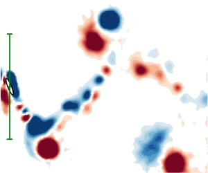
 $y$ plane. The blue and red contours represent clockwise and anti-clockwise vorticity, respectively. The black dot at the far left denotes the body centre position of the cylinder and the green vertical line between two horizontal bars indicates the peak-to-peak vibration amplitude. A single vortex is shed every half-cycle as part of the observed 2S wake mode, with additional vorticity in a zigzag pattern between the counter-rotating vortex pair forming a secondary vortex street (SVS).

Evolution of phase-averaged vorticity contours for control law parameters  $K_p^* = 2.39 \times 10^{-2}$ and
 $\phi _d = 178^\circ$ at
 ${U^*} = 5.0$ (Regime II). Although the SVS is more linear, does not persist as far downstream of the body and is more connected to the 2S vortices, the wake pattern is almost identical to figure 9 when no rotation is imposed. More details can be found in the caption of figure 9.

Sample time traces of the cylinder response at different reduced velocities and control law parameters selected from the three wake-body synchronisation regimes: (a)  $\{{U^*},K_p^*,\phi _d\} = \{5.0,2.39 \times 10^{-2},178^\circ \}$ (II – with control); (b)
 $\{{U^*},K_p^*,\phi _d\} = \{5.0,0,0^\circ \}$ (II – no control); (c)
 $\{{U^*},K_p^*,\phi _d\} = \{7.0,1.36\times 10^{-1},301^\circ \}$ (IV); and (d)
 $\{{U^*},K_p^*,\phi _d\} = \{8.5,3.80,18^\circ \}$ (V). Note that the time is normalised by
 ${{f_{nw}}}$, namely
 $\tau = t{{f_{nw}}}$.

In figure 9, the evolution of the vorticity shed by the elliptical cylinder with no imposed rotation (i.e.  $K_p^* = 0$) bears a marked resemblance to that first reported by Lo et al. (Reference Lo, Hourigan, Thompson and Zhao2023). The main wake structure is the 2S mode (Williamson & Roshko Reference Williamson and Roshko1988), which comprises two large counter-rotating vortices that are shed from either side of the cylinder per oscillation cycle. These large vortices are associated with the dominant frequency component of the vortex shedding process and the body vibration (see the PSD contours of
 ${f^*_{C_y}}$ and
 ${f^{*}_y}$) at the natural frequency
 ${{f_{nw}}}$. In addition, as the elliptical cylinder moves rapidly in the transverse direction between its extreme positions, it acts like an elliptical airfoil at a non-zero angle of attack and forms a wake, which manifests as a zigzag vorticity pattern that is particularly apparent in the near wake. The remnants appear between the two widely separated single vortices of the 2S mode. Termed an SVS, Lo et al. (Reference Lo, Hourigan, Thompson and Zhao2023) showed that this wake appears as a coalescence of vortices that resemble a local von Kármán vortex street. We also note that this structure shows similarities to the ‘coalescence’ wake pattern previously identified by Wang et al. (Reference Wang, Du, Zhao, Thompson and Sun2020) for a flapping NACA0012 airfoil.
Although the main features of the wake structure are still present even when the ideal control law parameters are applied, the increase in the vibration amplitude arises from modifications to their strength and position relative to the elliptical cylinder. From figure 10, which shows the steady-amplitude oscillation for  $K_p^* = 2.39 \times 10^{-2}$ and
 $\phi _d = 178^\circ$, the SVS is weaker (i.e. the SVS is thinner and does not persist as far downstream compared with the case with no axial rotation), with the largest structural difference occurring in the near wake when the cylinder approaches the peak displacement of the oscillation cycle. As opposed to the
 $K_p^* = 0$ case where the SVS is predominately a separate entity from the main 2S vortices, when the ideal control is imposed (figure 10), the same sign SVS vorticity remains connected and contributes to the 2S vortices whilst the body accelerates away from the peak displacement. It should be noted that the attachment of the SVS to the 2S vortices in figure 10 is not amplitude-dependent, as the wake structure is nearly identical for all
 ${U^*}$ cases evaluated within the reduced velocity range of interest for this section. Furthermore, due to the similarity in orientation angle, this attachment can also be observed between the anti-clockwise vortex of the 2S mode and the SVS for the FIV of the
 $\varepsilon = 5$ cylinder set at
 $\theta = 2.5^\circ$ and a reduced velocity of
 ${U^*} = 5$ (see figure 9 of Lo et al. Reference Lo, Thompson, Hourigan and Zhao2024b).
The increased vibration amplitude and the associated changes in the SVS when axial rotation is imposed can be further explored by considering the incident flow relative to the bluff body in motion. Due to the behaviour of the thin elliptical cylinder acting as a lift-generating airfoil (see Lo et al. Reference Lo, Hourigan, Thompson and Zhao2023) over its transverse motion, it is useful to characterise the flow in the following discussion based on the angle of attack  $\alpha$. As shown in figure 12,
 $\alpha$ is taken to be the angle between the relative flow (
 $U_{rel} = U\boldsymbol {i} +\dot {y}\boldsymbol {j}$, where
 $\boldsymbol {i}$ and
 $\boldsymbol {j}$ are unit vectors in the
 $x$ and
 $y$ direction, respectively) and the semimajor axis, and is defined as
 \begin{equation} \alpha = \arctan{\left(\frac{U}{\dot{y}(t)}\right)} + \theta = \arctan{\left(\frac{U}{\dot{y}(t)}\right)} + K_p^*y^*\left(t+\frac{\phi_d}{2{\rm \pi} f}\right), \end{equation}
when using the control law outlined in (2.5). From figure 13(a), which shows the minimum  $\alpha$ value achieved by the body as a function of
 ${U^*}$, the minimum angle of attack when the ideal control law was imposed (i.e. for the low gain peak) remains relatively constant over the range
 ${U^*} \leqslant 6$ with a mean of
 $\alpha _{min} =12.5^\circ$. This angle of attack causes the flow around the elliptical cylinder to generate strong lift as it reaches its maximum speed whilst limiting separation to the rear section of the body. The resulting vortex shedding results in the formation of an SVS that bears a marked resemblance to the vortex shedding from airfoils at an angle of attack (Gupta et al. Reference Gupta, Zhao, Sharma, Agrawal, Hourigan and Thompson2023).
Schematic of the elliptical cylinder moving upwards with a body velocity of  $\dot {y}$ and a body orientation angle of
 $\theta$. Here, the angle between the instantaneous relative flow
 $U_{rel}$ and the semimajor axis is given by
 $\alpha$.

(a) Minimum angle of attack (with respect to the relative flow  $U_{rel}$) achieved by the cylinder as a function of reduced velocity for the low-gain peak (red) and when no control is applied (black). (b) Angle of attack time trace at the low-gain peak (
 $K_p^* = 2.39 \times 10^{-2}$ and
 $\phi _d = 178^\circ$) when
 ${U^*} = 5.0$ and without control when
 ${U^*} = 5.4$ (corresponding to the non-rotating cylinder with a nearly identical
 ${A^{*}}$ value).

Interestingly, if the FIV dynamics for the  ${U^*}$ range investigated in this section was purely driven by a galloping-like movement-induced instability, one might expect the phase difference between the axial rotation and
 $y$ displacement signal to either be approximately
 $90^\circ$ or
 $270^\circ$. This is due to the modification in the angle of attack
 $\alpha$ being maximised (for a given non-zero
 $K_p^*$ value) over the oscillation period (i.e. as the cylinder travels from one peak displacement position to the next) for the two phase differences angles. However, with the FIV dynamics also seeing contribution from VIV, an analysis of the energy transfer between the cylinder and the fluid flow is needed to determine the physical mechanism that allows the axial rotations (imposed by the ideal control law) to maximise the oscillation amplitude.
Figure 14(a) shows the displacement and the energy transfer between the cylinder and the fluid over three oscillations for the representative case of  ${U^*} = 5$ when the ideal control law is applied. Time traces corresponding to approximately the same vibration amplitude and net energy transfer when no rotation is imposed (i.e.
 ${U^*} = 5.4$) are also presented in figure 14(b). To ensure a fair comparison between the two cases, the rate of energy transfer is characterised by
 $C_P{U^*}^3$ (since it is proportional to the dimensional energy transfer rate), where
 $C_p = F_y(t)\cdot \dot {y}(t)/(\tfrac {1}{2}\rho U^3bL)$ is the power coefficient. Because the fluid force and the body displacement is approximately in phase (i.e.
 $\phi _y \approx 10^\circ$ from Lo et al. Reference Lo, Thompson, Hourigan and Zhao2024b) for Regime II, energy is removed from the oscillating system when the cylinder is travelling away from the peak displacement position as observed in figure 14. Energy is then input back into the system by the fluid as the cylinder moves from zero displacement (i.e.
 $y^* = 0$) to the opposite peak displacement position. Net energy transfer to the body over a cycle is positive to match the loss from non-zero structural damping. Interestingly, although the average energy transfer (and hence vibration amplitude) is almost identical for figures 14(a) and 14(b), the peak positive and negative energy transfer when rotation is imposed is larger in magnitude when compared with the case when no control as applied.
Time trace of the body displacement and instantaneous energy transfer (in total and decomposed into the contribution from lift and drag) between the cylinder and fluid for (a)  $\{{U^*},K_p^*,\phi _d\} = \{5.0,2.39 \times 10^{-2},178^\circ \}$ and (b)
 $\{{U^*},K_p^*,\phi _d\} = \{5.4,0,0^\circ \}$. Note that the right and left axes of panels (a) and (b), respectively, refer to
 $C_P{U^*}^3$ and are of the same scale.

By considering the elliptical cylinder as an airfoil, further insight into the dynamics can be gained by decomposing the energy transfer into lift and drag components. Here, lift and drag are defined as the force perpendicular and parallel to the relative flow  $U_{rel}$, respectively. Their relationship with the streamwise
 ${{C_{x}}}$ and transverse
 ${{C_{y}}}$ forces is defined as
 $$\begin{gather} {{C_{L}}} = {{C_{y}}}\sin{(\alpha-\theta)}+{{C_{x}}}\cos{(\alpha-\theta)}, \end{gather}$$
 $$\begin{gather}{{C_{D}}} = {{C_{x}}}\sin{(\alpha-\theta)}-{{C_{y}}}\cos{(\alpha-\theta)}. \end{gather}$$
Manipulating these expressions allows the power coefficient to be expressed as
 \begin{equation} C_p = C_{p,L} + C_{p,D} = \frac{\dot{y}}{U}\left({{C_{L}}}\sin{(\alpha-\theta)} + (-{{C_{D}}}\cos{(\alpha-\theta)})\right), \end{equation}
where  $C_{p,L}$ and
 $C_{p,D}$ are the components of the total power coefficient due to the lift and drag forces, respectively. By comparing figures 14(a) and 14(b), it becomes clear that although the peak rate of energy loss due to drag remains roughly the same, the imposed axial rotation results in the same vibration amplitude with a smaller lift contribution by decreasing the rate of energy loss from the drag as the cylinder moves from
 $y^* =0$ to the point of peak displacement. To achieve this,
 $\phi _d$ of the control law, which dictates the period within the oscillation cycle where the modification to
 $\alpha$ occurs, was found to be near
 $180^\circ$ by the optimisation algorithm (figure 8a). The above conclusions agree well with figure 13(b), where the decrease in the rate of energy loss aligns with a reduction in the angle of attack. With a lower angle of attack increasing the flow attachment when the cylinder moves from
 $y^* =0$ to its position of peak displacement, it is also consistent with the SVS maintaining the connection to the main 2S vortices (figure 10) when the ideal control law is applied. Additionally, as the decrease in
 $\alpha _{min}$ between the two cases in figure 13(b) is only approximately
 $0.88^\circ$, it further establishes the sensitivity of the elliptical cylinder to the location in the oscillation period where the minimum angle of attack occurs.
To visualise this sensitivity of the FIV of the thin elliptical cylinder to axial rotation, figure 15 shows the  $C_L - C_D$ Lissajous plots for the two cases presented in figure 14:
 ${U^*} = 5.0$ when the ideal control law is imposed and
 ${U^*} = 5.4$ with no applied rotation. Since both instances have approximately the same vibration amplitude, it is perhaps surprising that the topology of the
 $C_L - C_D$ Lissajous plots are significantly different. Although the range of lift coefficients over an oscillation cycle is similar for both cases, introducing axial rotation as imposed by the ideal control law results in a decrease in the minimum drag coefficient experienced by the cylinder regardless of its direction of travel. This concurs with the observation of a weaker SVS in figure 10 since Lo et al. (Reference Lo, Hourigan, Thompson and Zhao2023) showed that this structure induces a ‘
 $\ldots$ “drag”-like force that impedes the motion of the cylinder along the
 $y$-axis’. Furthermore, there is less overlap in the lines of the
 $C_L - C_D$ plot when no rotation is applied (figure 15b), indicating an increased variation in the evolution of the lift and drag forces over each oscillation cycle as compared with figure 15(a). We also note that the difference between the dynamics of the elliptical cylinder moving upwards as opposed to moving downwards is exacerbated when the ideal control law is applied; this amplification is attributed to the
 $\phi _d$ generally not taking symmetric values (i.e.
 $\phi _d = 0^\circ, 90^\circ, 180^\circ$ or
 $270^\circ$).
 $C_L - C_D$ Lissajous plots for (a)
 $\{{U^*},K_p^*,\phi _d\} = \{5.0,2.39 \times 10^{-2},178^\circ \}$ and (b)
 $\{{U^*},K_p^*,\phi _d\} = \{5.4,0,0^\circ \}$ over three oscillation cycles. Here,
 $y\uparrow$ denotes the part of the vibration where the cylinder is travelling from negative to positive peak displacement, while
 $y\downarrow$ denotes the cylinder travelling in the opposite direction.

3.1.2. ${U^*} \geqslant 6.5$ (Regime IV)

As shown in figure 5 for the reduced velocity range  $6.5\leqslant {U^*}\leqslant 8.5$, imposing axial rotation (corresponding to the low-gain peak) causes Regime III and the desynchronised region to be replaced by a previously unseen type of wake-body synchronisation. Hereafter referred to as Regime IV, the vibration amplitude of this regime is characterised by an initial sharp decrease in amplitude with reduced velocity before plateauing to
 $A^* \approx 2.8$ for
 ${U^*} \geqslant 7$. Interestingly, the frequency response of this new regime bears more similarities to Regime II than Regime III, with the presence of a weak second harmonic and a strong third harmonic component of the transverse and vortex fluid forcing detected in addition to the dominant frequency contribution at the natural frequency (
 ${f^*_{C_y}} \simeq {f^*_{C_{v}}} \simeq 1$). The low minimum angle of attack magnitude (figure 13a), the total phase remaining close to zero and the substantially larger oscillation amplitude than seen in Regime III indicate that the dynamics of the dominant lock-in regime over this reduced velocity range appears to be also partly driven by a movement-induced instability when the control law is imposed. This contrasts with the FIV response when no rotation is applied (i.e. Regime III), which is more consistent with pure VIV. For Regime III, it is noted there is a lack of a zigzag structure in the wake shedding, an almost complete absence of second and third harmonics in the fluid forcing (Lo et al. Reference Lo, Hourigan, Thompson and Zhao2023), and, importantly, a jump in the total phase from close to zero to close to 180
 $^\circ$ consistent with that observed for the lower to upper branch transition in the generic circular cylinder case (Williamson & Govardhan Reference Williamson and Govardhan2004). Consequently, the largest amplitude increases are observed over this
 ${U^*}$ range due to the imposed rotation inducing the movement-induced vibration, thereby allowing wake-body synchronisation to occur over the entire explored reduced velocity range (i.e.
 $3 \leqslant {U^*} \leqslant 8.5$).
To gain a further understanding of this new type of coupling between VIV and the galloping-like movement-induced vibration, PIV conducted for the representative case of  ${U^*} = 7.0$ (with control parameters
 $K_p^* = 1.36 \times 10^{-1}$ and
 $\phi _d = 301^\circ$) is presented in figure 17. As expected from the frequency response of the fluid forcing in figure 5, the wake structure for Regime IV is dissimilar to Regime III with the clear appearance of elliptical airfoil wakes from the body as it moves between positive and negative maximum displacements, i.e. displaying SVSs, similar to those found for Regime II. However, due to the rotation from negative to positive orientation angle as the cylinder approaches its positive peak displacement, the last anti-clockwise vortex in the set of small vortices that make up the SVS is disproportionately larger than the others. While the flow advects this region of vorticity, the last anti-clockwise vortex separates from the SVS and becomes an independent secondary vortex that travels downstream with (but is weaker than) the top main clockwise vortex. Due to the symmetry in the vortex shedding pattern, the above observations also apply (but in reverse) when the cylinder is at its negative peak displacement. As such, the resulting vortex pairs belong to a ‘2P’ wake formation (defined as two vortex pairs shed every oscillation cycle) in line with the naming convention proposed by Morse & Williamson (Reference Morse and Williamson2009a) and Williamson & Govardhan (Reference Williamson and Govardhan2004). Additionally, while the aforementioned wake pattern remains approximately the same for the low-gain peak over the reduced velocity range
 $6.5\leqslant {U^*}\leqslant 8.5$, we note that the secondary vortex of the 2P mode and its separation from the SVS becomes stronger and more clearly defined with
 ${U^*}$.
The presence of the SVS observed in figure 17 agrees well with the low angle of attack observed over the reduced velocity range  $6.5\leqslant {U^*}\leqslant 8.5$ in figure 16(a). We note that the minimum
 $\alpha$ value for Regime IV, which is lower than for Regime II, decreases with increasing
 ${U^*}$. Comparing the angle of attack time trace with
 $\arctan (U/\dot {y})$ for the representative case of
 ${U^*} = 7.0$ in figure 16(a), the small minimum
 $\alpha$ value is achieved by setting the phase difference of the control law to be near
 $\phi _d = 270^\circ$, concurring with figure 8(a).
Time trace of (a) the absolute angle of attack and  $\arctan (U/\dot {y})$, and (b) the body displacement and instantaneous energy transfer between the cylinder and fluid for
 $\{{U^*},K_p^*,\phi _d\} = \{7.0,1.36 \times 10^{-1},301^\circ \}$.

Evolution of phase-averaged vorticity contours for control law parameters  $K_p^* = 1.36 \times 10^{-1}$ and
 $\phi _d = 301^\circ$ at
 ${U^*} = 7.0$ (Regime IV). The main wake pattern is a 2P
 $_{o}$ wake mode consisting of two counter-rotating vortex pairs (with one vortex in the pair being weaker than the other) shed every oscillation cycle. Additional vorticity in the form of an SVS is also observed in between the 2P
 $_{o}$ wake, although the angle with respect to the
 $y$-axis is larger in magnitude compared with Regime II (see figures 9 and 10). More details can be found in the caption of figure 9.

The behaviour mentioned above may also explain why the low-gain peak in the amplitude response corresponding to Regime IV does not vary smoothly over the control parameter space  $\mathcal {B} = \{K_p^*, \phi _d\}$ but is instead discontinuous with changes in
 $K_p^*$ (figure 7b–f). This means that, with
 $\phi _d$ set to its ideal value (e.g.
 $301^\circ$ for
 ${U^*} = 7.0$), the vibration amplitude will increase with decreasing proportional gain until the low-gain peak is reached at the ideal
 $K_p^*$ value determined by Bayesian optimisation (e.g. 0.136 for
 ${U^*} = 7.0$). A sudden drop in
 ${A^{*}}$ occurs once the gain is decreased past this critical point. Therefore, since the proportional gain relates the oscillation amplitude to the amplitude of the axial rotation, a higher
 $K_p^*$ means that the angle of attack required for attached flow (and hence the onset of the movement-induced instability) can be reached at lower oscillation amplitudes. This, along with the
 $\phi _d$ values for this regime being generally closer to
 $270^\circ$ as compared with Regime II (with ideal control law imposed), suggests that the movement-induced instability plays a significant role in causing wake-body synchronisation over the reduced velocity range
 $6.5\leqslant {U^*}\leqslant 8.5$. Additionally, while the ability of the body to synchronise with the wake generally improves with the gain, the vibrational amplitude rises as
 $K_p^*$ is decreased. As such, the low-gain peak over the reduced velocity range
 $6.5 \leqslant {U^*}\leqslant 8.5$ can be considered to be the lowest gain value that can reach the minimum angle of attack shown in figure 13(a) while still able to achieve lock-in.
As the transverse fluid forcing is approximately in-phase with the body displacement (figure 4b), the energy transfer between the fluid and cylinder is similar to that for Regime II in that the  $C_p$ value in figure 16(b) is positive (i.e. energy is being input from the fluid) when the body is moving from
 $y^* = 0$ towards the position of peak displacement. However, when decomposing the power coefficient into its lift and drag components (see (3.2)–(3.4)),
 $C_{p,L}$ and
 $C_{p,D}$ were found to generally contribute minimally to the energy transfer for
 $\Delta \tau = 0.05$ after the cylinder has reached its peak displacement, with
 $C_{p,L}$ found to be slightly negative in value. This is in contrast to Regime II (figure 14), where the energy transfer due to the lift and drag (both of which closely resemble the absolute value of a sinusoidal function) is always positive and negative, respectively. The observed differences likely arise due to the larger and positive orientation angle when the cylinder is accelerating away from its positive peak displacement, resulting in smaller lift and drag forces. This observation concurs with the time traces in figure 11(c), where the low
 ${{C_{x}}}$ value between
 $\tau =0.25$ and
 $0.5$ (repeating every
 $\Delta \tau = 1$) is due to the direction of lift induced by the cylinder with a positive orientation angle being in the opposite direction to the
 $x$-axis. The same reasoning also holds as the cylinder is accelerating away from its negative peak displacement with a negative
 $\theta$ value. Furthermore, it is interesting to note that the energy transfer is in stark contrast to that of Regime III, with
 $\phi _y \approx 180^\circ$ (figure 4b) resulting in the net positive energy transfer to the cylinder occurring as the body moves from its peak displacement towards the
 $y^* = 0$ centreline.
3.2. Ideal control parameters for the high-gain peak (Regime V)
For reduced velocity in the range  $6.5 \leqslant {U^*} \leqslant 8.5$, a secondary peak in the oscillation amplitude was observed that was previously unseen for the
 $3 \leqslant {U^*} \leqslant 6$ cases, with the variation of the corresponding proportional gain and phase difference values as a function of
 ${U^*}$ presented in figure 8(b). Occurring for
 $K_p^* > 1$, as shown by the contour plots in figure 7(b–f) and belonging to a new wake-body synchronisation regime hereafter referred to as Regime V, this high-gain peak (represented by the green markers in figure 4a) is considered a local maximum since it is smaller in magnitude than the low-gain peak. The displacement and fluid force time traces of this regime for the representative
 ${U^*} = 8.5$ case (with control parameters
 $K_p^* = 3.80$ and
 $\phi _d = 18^\circ$) are presented in figure 11(d). In addition, the presence of the high-gain peak also shifts the range of phase difference between the rotation and the body displacement for minimal vibration from
 $0^\circ \leqslant \phi _d\leqslant 135^\circ$ (as described in § 3.1.1) to
 $90^\circ \leqslant \phi _d\leqslant 180^\circ$.
As a result of the axial rotation amplitude required for the high-gain peak exceeding  ${\rm \pi}$ (i.e. the cylinder achieving more than one complete rotation in a body oscillation cycle), the physical mechanisms causing the vibration amplification are hence different from those controlling Regimes II and IV. Instead of modifying the angle of attack to decrease the energy loss from drag forces acting on the cylinder during an oscillation cycle, the large axial rotations due to the high gain value indicate significant vorticity emission from the cylinder's surface. With the cylinder rotating in the same direction as the vorticity being shed, it increases the circulation intensity of the vortices and, as a result, the oscillation amplitude. Therefore, it appears likely that this vibration enhancement arises from the significant external energy input into the fluid–structure system by the servo motor imposing the axial rotations.
Since the frequency of both the transverse fluid and vortex forces occur just below the natural frequency in quiescent water,  ${{f_{nw}}}$, with a complete absence of any higher-order harmonics (see figure 18), it indicates that vortex formation is still very much coupled to the oscillation of the cylinder despite the body's high rotation rate caused by the large gain value. This is in contrast to the behaviour observed by Vicente-Ludlam et al. (Reference Vicente-Ludlam, Barrero-Gil and Velazquez2017) for
 ${U^*} > 15$ when
 $K_p^* = 1.2$ and
 $\phi _d = 0^\circ$, where the clear separation between the vortex shedding and body vibration frequency demonstrates that a galloping-like movement-induced instability predominately drives the oscillations. However, an exception to the above discussion about harmonics is the
 ${U^*} = 6.5$ case, where
 ${f^*_{C_y}} \simeq {f^*_{C_{v}}} \simeq 2.9$ frequency components are also observed. This is likely due to the proportional gain value of the true local maxima being outside the
 $K_p^* \leqslant 5$ range of interest in this study. Additionally, we note that the large body rotation rate representative of Regime V also causes weak harmonics to appear sporadically in the drag force frequency response as shown in figure 18(d).
Logarithmic-scale PSD contours of the (a) normalised vibration ( ${f^{*}_y}$), (b) transverse fluid force (
 ${f^*_{C_y}}$), (c) vortex force (
 ${f^*_{C_{v}}}$) and (d) streamwise force (
 ${f^*_{C_y}}$) frequencies as a function of
 ${U^*}$ for the high-gain peak (Regime V). In panels (a–c), the horizontal dashed line highlights the frequencies at
 ${f^{*}} \in \{1,2,3\}$, respectively, and the dash-dotted line represents the Strouhal frequency measured for a stationary cylinder. Note that the frequencies of the horizontal dashed and dash-dotted lines in panel (d) are doubled compared with their counterparts in panels (a–c).

As the transverse fluid forcing is approximately in phase with the body displacement (figure 4b), it also indicates that the Magnus effect does not drive the vibrations of Regime V. The Magnus effect results in a lift force that is perpendicular to the axis of rotation and acting in the direction of the side of the body rotating with the free stream flow. Since this phenomenon arises due to the pressure difference between the top and bottom sides of the body from the addition of momentum near the body's surface, the resultant force produced is hence proportional to the angular velocity  $\dot {\theta }$. Consequently, if a Magnus-force-like effect is the primary instigator of the vibration in Regime V, one would expect the peak transverse force
 $C_y$ to occur when
 $\dot {\theta }$ is greatest. As
 $\phi _d \approx 18^\circ$, the axial velocity, and by extension the transverse force
 $C_y$, should have a phase shift of approximately
 $108^\circ$ relative to the displacement signal (i.e.
 $\phi _y = 108^\circ$). However, with the fluid force being approximately in phase with the body displacement (i.e.
 $\phi _y \approx 0^\circ$), it implies that the Magnus force does not play a significant role in driving the oscillations and in the FIV dynamics of Regime V.
A greater understanding of the FIV dynamics can be gained by observing the wake structures shed by the cylinder. As shown by PIV results in figure 19 for the representative case of  ${U^*} = 8.5$, the large rotation rate of the cylinder in Regime V results in a vortex shedding pattern with a greater number of vortices that are generally less defined when compared with the other lock-in regimes (i.e. I, II, III and IV). Unexpectedly, while the wakes discussed so far in this study have been symmetric over an oscillation period, Regime V is the first type of wake-body synchronisation that results in an uneven number of vortices above and below the
 $y^* = 0$ centre line. From figure 19(b), this pattern is labelled a
 $T+P$ wake mode since a vortex pair (i.e.
 $P$) is shed as the cylinder is travelling downwards from the positive peak displacement and a triplet (i.e.
 $T$, consisting of a clockwise vortex situated above two anti-clockwise vortices positioned side-by-side) is shed as the cylinder travels upwards from the negative peak displacement. The pattern of
 $T+P$ has been previously observed by Wang et al. (Reference Wang, Du, Zhao and Sun2017) for a 2-degree-of-freedom flapping NACA0012 airfoil. While the vortices are shed in a wave-like manner similar to that observed by Vicente-Ludlam et al. (Reference Vicente-Ludlam, Barrero-Gil and Velazquez2018) for a circular cylinder with parameters
 $\{{U^*},K_p^*, \phi _d\} = \{17,1.875, 0^\circ \}$, the vortices are not shed independently at different points of the oscillation cycle. This is most evident by the clear vortices observed in figure 19, which are PIV phase-averaged fields based on the body displacement and velocity. Therefore, the presence of distinct vortices indicates that vorticity is consistently shed at particular points in the cylinder's oscillation cycle, further supporting the above conclusion that the observed dynamics is due to wake-body synchronisation.
Evolution of phase-averaged vorticity contours for control law parameters  $K_p^* = 3.80$ and
 $\phi _d = 18^\circ$ at
 ${U^*} = 8.5$ (Regime V). The shedding pattern is a
 $T+P$ wake mode characterised by one vortex triplet (consisting of one clockwise vortex situated above two counter-clockwise vortices) and one counter-rotating vortex pair. The black dashed line represents the past trajectory of the cylinder, with more details found in the caption of figure 9.

To summarise, the above observations have shown that the Magnus effect and the movement-induced instability are unlikely candidates to explain the dynamics of Regime V. However, with  ${f^{*}_y} \simeq {f^*_{C_y}} \simeq {f^*_{C_{v}}} \simeq 1$ and periodic vortex shedding occurring in figure 19, it suggests that Regime V is likely to be VIV-dominated with the resultant dynamics arising from the resonance between the body oscillation and the vortex shedding.
3.3. Adaptive gain for further vibration amplification
Although this study has shown that introducing the axial rotation imposed by the control law specified in (2.5) increases the vibration amplitude of the elliptical cylinder started from rest, Lo et al. (Reference Lo, Hourigan, Thompson and Zhao2023, Reference Lo, Thompson, Hourigan and Zhao2024b) found that even larger oscillations at higher reduced velocities could be sustained for a non-rotating cylinder (i.e.  $K_p^* = 0$) if the flow speed was continuously increased from minimum to maximum reduced velocity. This behaviour can be attributed to the cylinder being a ‘hard-oscillator’ (see Naudascher & Rockwell Reference Naudascher and Rockwell2005) as indicated by the amplitude response with increasing
 ${U^*}$ increments in figure 20(a), where large Regime II vibrations for
 ${U^*} >6.3$ can only occur when the initial amplitude is beyond a certain threshold. Therefore, the following question arises: can axial rotations be used as a method to excite Regime II oscillations for an elliptical cylinder initially at rest when the reduced velocity is above 6.3?
(a) Comparison of the amplitude response for an elliptical cylinder started from rest (filled black symbol) and when increasing  ${U^*}$ increments are used. The red marker with the black edge denotes the amplitude achieved with the adaptive gain control law, while the purely red marker represents the intermediate state (i.e. maximum
 $A^*$ achieved when
 $K_{p,a}^*$ =
 $K_p^*$). (b) Amplitude contour plot as a function of adaptive gain control law parameters
 $A_{ref}^*$ and
 $\lambda$, with the black star indicating maximum achievable amplitude (
 ${A^{*}} = 5.87$). (c) Time trace of
 $y^*$,
 $K_{p,a}^*$ and
 $\theta$ over 200 non-dimensional time units
 $\tau$ for the cylinder started from rest when the adaptive gain control law is applied. Here,
 $\{K_p^*, \phi _d, \lambda, A^*_{ref}\} = \{0.236, 301^\circ, 2.35, 2.16\}$.

Since the physical cause of the elliptical cylinder acting as a hard oscillator is due to an absence of (semi-)attached flow around it (producing lift) when the body velocity is below a critical value (Lo et al. Reference Lo, Hourigan, Thompson and Zhao2023), the strategy of inducing Regime II oscillations can hence be broken down into two main steps. First, axial rotations are used to establish flow attachment around the cylinder. Once established, the second step will be to ensure that this attachment is sustained even as the proportional gain approaches zero, thereby resulting in an oscillation amplitude that is identical to the amplitude response when increasing  ${U^*}$ increments are used (denoted by hollow markers in figure 20a). With the control law proposed in (2.5) only able to achieve the first objective (see § 3.1.2), we found that the desired result could be attained for the representative
 ${U^*} = 7$ case with appropriate modification of the proportional gain term to the following form (hereafter known as adaptive gain):
 \begin{equation} K_{p,a}^*(A^*;\lambda,A^*_{ref}) = K_{p}^*\cdot\min\left(\exp{[-\lambda(A^*-A^*_{ref})]},1\right), \end{equation}
where  $\lambda$ is the decay rate,
 $K_{p,0}$ is the initial gain constant and
 ${A^{*}}_{ref}$ is the amplitude where exponential decay begins (i.e. the intermediate state). Here, we have included the vibrational amplitude as an additional input into the control law, with
 $K_{p,a}$ decaying exponentially with
 $A^*$. The choice of the exponential function arises from the sensitivity of the amplitude response to small orientation angles as shown by Lo et al. (Reference Lo, Thompson, Hourigan and Zhao2024b), where a
 $\sim$ 60 % decrease in the maximum vibration amplitude was observed when an angle of
 $\alpha = 3.5^\circ$ was introduced. Furthermore, by leveraging the gain and phase difference parameters previously obtained in § 3.1.2 for
 ${U^*} =7$ (i.e. the low-gain peak) as the intermediate state, a greedy approach can be used since the adaptive gain will only require optimisation with respect to
 ${A^{*}}_{ref}$ and
 $\lambda$. As such, this will simplify the problem by minimising the dimensionality of the search space explored by the Bayesian optimisation algorithm to find the optimal control law.
To implement this adaptive gain,  $K_{p,a}^*$, the
 $A^*$ input signal was measured to be
 $\sqrt {2}A^*_{rms}$, with
 $A^*_{rms}$ being the moving root-mean-square of the normalised displacement signal over the period
 $\Delta \tau = 1$ (i.e.
 $1/{{f_{nw}}}$ seconds). Due to the sensitivity of the low-gain peak to the proportional gain value, the control law parameter values were taken as
 $\{K_p^*, \phi _d\} = \{0.236, 301^\circ \}$ (resulting in an amplitude of
 ${A^{*}} = 2.18$) to ensure consistent lock-in that is independent of experimental conditions. Again, the multi-stage Bayesian optimisation approach described in § 2.3 was used to optimise the parameters of the adaptive gain
 $K_{p,a}^*$ and the decay rate
 $\lambda$ with respect to the cost function (2.6). In the first stage, 100 iterations were conducted over the range
 $A^*_{ref} \in [0, 2.18]$ and
 $\lambda \in [0, 6]$ with an exploration ratio of
 $t_\sigma = 1 \times 10^{12}$. A further 100 iterations were completed over a smaller range of decay values
 $\lambda \in [0, 3]$ using an exploration ratio of
 $t_\sigma = 0.5$, before finally conducting a final 25 iterations with an exploration ratio of
 $t_\sigma = 0$. The resultant contour plot of the vibration amplitude as a function of the adaptive gain parameters
 $\lambda$ and
 $A^*_{ref}$ is presented in figure 20(b).
From the contour plot, we can see that enabling the gain to vary with the vibration amplitude allows the large vibrations of Regime II to be excited for an elliptical cylinder started from rest. This could not be achieved with the constant gain law (i.e.  $\lambda = 0$) due to the ability of the body to synchronise with the wake increasing with
 $K_p^*$, at the expense of oscillation amplitude that can be achieved. The maximum obtained vibration amplitude of
 ${A^{*}} = 5.87$ is marked by the black star and occurs when {
 $K_p^*$,
 $\phi _d$,
 $\lambda$,
 $A^*_{ref}\} = \{0.236, 301^\circ, 2.35, 2.16\}$. Interestingly, a large diagonal band of high
 $A^*$ values can also be observed in figure 20(b), thereby indicating the robustness of the adaptive gain approach since large vibrations can be excited over a range of
 $A^*_{ref}$ and
 $\lambda$ values.
To understand the dynamics of the elliptical cylinder started from rest, figure 20(c) presents the evolution of the body displacement, adaptive gain and orientation angle over 200 non-dimensional time units,  $\tau = t{{f_{nw}}}$, when the optimised control law is imposed (
 $\lambda = 2.35$,
 $A^*_{ref} = 2.16$). The evolution of the wake, as determined using time-resolved PIV (conducted using 3100 image pairs at a frequency of 30 Hz), is also presented in Movie 1 and is available at https://doi.org/10.1017/jfm.2024.1128. Starting from
 $\tau = 0$ when the cylinder is at rest (i.e.
 $\theta = 90^\circ$), the body is rotated to
 $\theta = 0^\circ$ and axial rotation is imposed. As
 ${A^{*}} < A^*_{ref}$ from
 $\tau = 1\text { to }47.06$, the gain remains static and the system evolves similarly to that of the constant-gain control law (§ 2.2). Once
 $A^*_{ref}$ has been reached and the rotation amplitude reaches a maximum of
 $29.3^\circ$, the exponential decay of
 $K_{p,a}^*$ with vibration amplitude begins. Since wake-body synchronisation has already been established and flow streamlining is occurring around the body, a reduction in
 $K_{p,a}^*$ corresponds to further rises in
 $A^*$, which in turn results in a further decrease in
 $K_{p,a}^*$. This positive feedback loop then continues until a steady vibration amplitude of
 ${A^{*}} = 5.87$ (corresponding to an approximately 110 % increase compared with the low-gain peak for the same
 ${U^*}$ value) is reached when
 $\tau \approx 117.5$. However, care must also be taken to maintain the flow attachment around the body as the rotational amplitude is decreased. If
 $K_{p,a}^*$ is decreased too early (i.e.
 $A^*_{ref} \in [0,0.75]$) or too rapidly (
 $\lambda \gtrsim 3$), as indicated by the low-amplitude regions in figure 20(c), the elliptical cylinder will not be able to consistently sustain the necessary flow condition required to increase the vibration amplitude until
 ${A^{*}} = 5.87$ is attained. Furthermore, since the rotational amplitude reaches a value of near-zero (i.e.
 $A_\theta \approx 0.1^\circ$) at
 $\tau \approx 104$, it indicates that the cylinder can reach an amplitude of
 ${A^{*}} = 5.87$ without imposing any further axial rotation once
 $A^* \approx 5.35$ is achieved and attached flow is established around the cylinder.
Therefore, we can conclude that the control law with adaptive gain allows the elliptical cylinder to act as a ‘soft’ oscillator (i.e. exciting oscillations corresponding to Regime II from rest) when  ${U^*} = 7.0$. Although this has only been validated for one reduced velocity, it is expected that the proposed approach will also work for
 $6.3 <{U^*}< 8.5$ values as well given the low-gain peak (i.e. indicating the presence of flow attachment) in figure 4(a) when the constant-gain control law is used. In addition, once the high-amplitude limit cycle belonging to Regime II is reached, it may also be possible to switch back to the normal control law described in (2.5) for further amplitude enhancement. However, this is outside the scope of the current study given the current limits of our water channel facilities.
From an engineering perspective, the success of the control law with adaptive gain has potential implications for energy harvesting applications since increasing the vibration amplitude of the cylinder (for a fixed damping value) will increase the power output from the system. With the body subjected to external perturbations in the real world (e.g. flow velocity fluctuations and collisions with foreign objects) that may reduce the vibration amplitude to an unrecoverable value, the control strategy can be used to restore the large oscillations of Regime II efficiently due to the imposed rotation also being dependent on  $A^*$. Beyond the possible use as a vibration recovery mechanism, it would also be interesting to explore the capability of the proposed adaptive gain approach in attenuating both the effect of FIV and unsteady flow (arising from external upstream disturbances) on the body dynamics. With appropriate modification to the cost function (2.6), this could be applied to transient problems like minimising the impact of unsteady aerodynamics from wing–gust encounters on the lift generation performance of airfoils (see Fukami & Taira Reference Fukami and Taira2023; Sedky et al. Reference Sedky, Gementzopoulos, Lagor and Jones2023) and, as such, should be explored as part of a future study.
4. Conclusions
In our study, Bayesian optimisation was used to identify the control law that maximises (both locally and globally) the FIV of an elastically mounted elliptical cylinder (with an elliptical ratio of  $\varepsilon =5$ and a mass ratio of
 ${{m^{*}}} = 53$) started from rest across a reduced velocity range of
 $3.0 \leq {U^*} \leq 8.5$. Axial rotation was used as the primary actuation mechanism where the relationship between the cylinder orientation and displacement was determined by the proportional gain,
 $K_p^*$, and phase difference,
 $\phi _d$, parameters of the control law (2.5). By modifying the fluid–structure interaction, the resulting amplitude response when control was applied was larger than the non-rotating case for all
 ${U^*}$ values considered in this study. Specifically, an average increase of
 $14.7\,\%$ (with the maximum axial rotation amplitude required being less than
 $12.5^\circ$) was observed over a reduced velocity range of
 $3.0 \leq {U^*} \leq 6$, with the imposed rotation extending the wake-body synchronisation across the entire
 ${U^*}$ range of interest as opposed to
 $3.0 \leq {U^*} \leq 7.4$ for the non-rotating cylinder.
Furthermore, three wake-body synchronisation regimes (II, IV, V) were identified when active control was applied; two of which, to the authors’ knowledge, have not been previously reported. Although the wake pattern for Regime II did not significantly change when active control was applied, the length of the SVS – the vortex street from the body as it moves up and down between maximum displacements – was observed to increase with its persistence in the far wake reduced. This change was attributed to the phase difference between the rotation and transverse displacement being approximately  $180^\circ$, resulting in a lower angle of attack and hence increased flow attachment as the cylinder moves from
 $y^* = 0$ to the peak displacement point. Interestingly, while the 2S wake mode is the primary flow pattern for the non-rotating elliptical cylinder, the main vortex-shedding structure of Regime IV is a 2P wake mode. As evidenced by the additional presence of the SVS and the low total phase, the FIV dynamics of this regime seems to show contributions from both VIV and movement-induced vibration, again with the fluid forcing being strongly in phase with the body displacement (i.e.
 $\phi _y < 20 ^\circ$). However, Regime V is characterised by the asymmetric
 $T+P$ mode and is the only wake-body synchronisation regime in this study marked by axial rotations with an angular displacement amplitude greater than
 ${\rm \pi}$ radians. Unlike Regimes II and IV where the large oscillations can be attributed to the attached flow around the cylinder caused by the low minimum angle of attack, Regime V's dynamics is predominantly driven by the significant body rotation injecting circulation from the cylinder surface into the shed vortices.
Although the control law increases both the vibration amplitude and the  ${U^*}$ range where wake-body synchronisation occurs as compared with the non-rotating cylinder started from rest, the resulting oscillations are less than the non-rotating case for increasing
 ${U^*}$ increments when
 $6.3 < {U^*} < 7.1$. Given that the elliptical cylinder is a ‘hard oscillator’ over this reduced velocity range, we further propose an adaptive proportional gain (i.e. varies as a function of
 ${A^{*}}$) which overcomes this limitation by providing the cylinder with the required initial vibration amplitude to sustain the large Regime II oscillations. As the rotation magnitude depends on the cylinder's current oscillation amplitude, the approach allows Regime II oscillations to be maintained in an energy-efficient manner for flow speeds where the body acts as a hard oscillator. This has potential implications for renewable energy applications since, for practical applications, the cylinder is likely to be initially at rest and/or may be subjected to external perturbations that may reduce the vibration amplitude to an unrecoverable value.
However, the success of the adaptive gain has also highlighted the potential for even further vibration enhancements to be gained from rotations imposed by more sophisticated control strategies. Applying deep learning methodologies for FIV maximisation could be an interesting avenue to explore in future studies, especially for systems that see the joint occurrence of VIV and movement-induced instability. For energy harvesting applications, the effect of, and the manner in which, damping is applied to the rotating cylinder should also be investigated. Additionally, as energy is required to drive the motor, the net power output from this FIV system can be maximised by making the active control strategy more efficient through the incorporation of angular rotation as a term in the cost function.
Supplementary movie
Supplementary movie is available at https://doi.org/10.1017/jfm.2024.1128.
Movie caption: Time-resolved particle image velocimetry showing the evolution of the wake shed by the elliptical cylinder started from rest when the optimised adaptive control law is imposed ( $K_p^* = 0.236$,
 $\phi _d = 301^{\circ }$,
 $\lambda = 2.35$,
 $A_{ref}^* = 2.16$).
Funding
This work was supported by the Australian Research Council (J.Z., Discovery Early Career Researcher Award DE200101650; K.H. and J.Z., Discovery Project DP210100990; and M.C.T., Discovery Project DP190103388).
Declaration of interests
The authors report no conflict of interest.


 Open access

