2.1 Classical equations

In the framework of the classical description of miscible liquids, the governing equations, that determine the hydrodynamics of two isothermal incompressible miscible liquids, read (see Gaponenko et al. Reference Gaponenko, Volpert, Zen’kovskaya and Pojman2006; Gaponenko & Shevtsova Reference Gaponenko and Shevtsova2010; Gaponenko et al. Reference Gaponenko, Torregrosa, Yasnou, Mialdun and Shevtsova2015a )

(2.1) $$\begin{eqnarray}\displaystyle & \displaystyle \frac{\unicode[STIX]{x2202}\boldsymbol{u}}{\unicode[STIX]{x2202}t}+(\boldsymbol{u}\boldsymbol{\cdot }\unicode[STIX]{x1D735})\boldsymbol{u}=-\unicode[STIX]{x1D735}\unicode[STIX]{x1D6F1}_{1}+\unicode[STIX]{x0394}\boldsymbol{u}-\frac{Gs}{Sc}(\boldsymbol{w}\boldsymbol{\cdot }\boldsymbol{w}_{0})\unicode[STIX]{x1D735}C, & \displaystyle\end{eqnarray}$$

(2.2) $$\begin{eqnarray}\displaystyle & \displaystyle \frac{\unicode[STIX]{x2202}C}{\unicode[STIX]{x2202}t}+(\boldsymbol{u}\boldsymbol{\cdot }\unicode[STIX]{x1D735})C=\frac{1}{Sc}\unicode[STIX]{x0394}C, & \displaystyle\end{eqnarray}$$

(2.3) $$\begin{eqnarray}\displaystyle & \displaystyle \unicode[STIX]{x1D735}\boldsymbol{\cdot }\boldsymbol{u}=0. & \displaystyle\end{eqnarray}$$

These are the Navier–Stokes equation, the equation for the diffusive transport and the continuity equation. For simplicity, dependencies of viscosity and diffusion coefficients on concentration are disregarded. These are the time-averaged equations that are written for the time-average quantities, namely, $\boldsymbol{u}$ is the time-averaged velocity, $\unicode[STIX]{x1D6F1}_{1}$ is the modified pressure that is determined from an incompressibility constraint, and $C$ is the concentration that is defined as the mass fraction of one of the liquids in a mixture. It is assumed that the container that encloses the mixture is subjected to the high-frequency vibrations, with the direction given by the vector $\boldsymbol{w}_{0}=\boldsymbol{i}$ , where $\boldsymbol{i}$ is a unit vector along the $x$ -axis. The Navier–Stokes equation includes the vibrational force. The vector $\boldsymbol{w}$ determines the spatial variations in the pulsational velocity and it is defined by equations,

(2.4) $$\begin{eqnarray}\unicode[STIX]{x1D735}\times \boldsymbol{w}=\boldsymbol{w}_{0}\times \unicode[STIX]{x1D735}C,\quad \unicode[STIX]{x1D735}\boldsymbol{\cdot }\boldsymbol{w}=0.\end{eqnarray}$$

The above equations (2.1)–(2.4) are written in the non-dimensional form. The following scales were used to non-dimensionalise the equations

(2.5a-d ) $$\begin{eqnarray}u_{\ast }=\frac{\unicode[STIX]{x1D702}_{\ast }}{\unicode[STIX]{x1D70C}_{\ast }L_{\ast }};\quad \unicode[STIX]{x1D70F}=\frac{L_{\ast }}{u_{\ast }};\quad \unicode[STIX]{x1D6F1}_{1\ast }=\unicode[STIX]{x1D70C}_{\ast }u_{\ast }^{2};\quad w_{0\ast }=a\unicode[STIX]{x1D714};\quad w_{\ast }=\unicode[STIX]{x1D719}a\unicode[STIX]{x1D714}.\end{eqnarray}$$

Here, for the typical velocity and typical time scale, $u_{\ast }$ and $\unicode[STIX]{x1D70F}$ , we adopt the convective scales; $\unicode[STIX]{x1D702}_{\ast }$ and $\unicode[STIX]{x1D70C}_{\ast }$ are the typical viscosity and density that may be taken as the average values of these quantities for pure components of a mixture; and the length scale $L_{\ast }$ is equal to the container’s height. The scales of the pulsational fields $\boldsymbol{w}_{0}$ and $\boldsymbol{w}$ are denoted by $w_{0\ast }$ and $w_{\ast }$ . The scale of pressure field $\unicode[STIX]{x1D6F1}_{1}$ is given by $\unicode[STIX]{x1D6F1}_{1\ast }$ .

The governing equations include two non-dimensional parameters, these are the Schmidt and Gershuni numbers,

(2.6a,b ) $$\begin{eqnarray}Sc=\frac{\unicode[STIX]{x1D702}_{\ast }}{\unicode[STIX]{x1D70C}D_{\ast }},\quad Gs=\frac{\unicode[STIX]{x1D70C}_{\ast }\unicode[STIX]{x1D719}^{2}(a\unicode[STIX]{x1D714})^{2}L_{\ast }^{2}}{2\unicode[STIX]{x1D702}_{\ast }D_{\ast }}.\end{eqnarray}$$

(The Gershuni number is also frequently called the vibrational Rayleigh number.)

The governing equations are supplemented with the following boundary conditions,

(2.7a-c ) $$\begin{eqnarray}\boldsymbol{u}=0,\quad w_{n}=0,\quad \frac{\unicode[STIX]{x2202}C}{\unicode[STIX]{x2202}n}=0.\end{eqnarray}$$

On all walls of a container, we impose the no-slip boundary condition for the average velocity, the no-penetration condition for the pulsational velocity (the equations for pulsations are inviscid, and hence one may not impose any restrictions on the tangential component of the pulsational flow) and the last boundary condition excludes the diffusive transport across the walls.

For the numerical solution of the 2-D problem the above equations (2.1)–(2.4) are convenient to re-write in terms of the vorticity ( $\unicode[STIX]{x1D6FA}=\unicode[STIX]{x2202}u_{x}/\unicode[STIX]{x2202}y-\unicode[STIX]{x2202}u_{y}/\unicode[STIX]{x2202}x$ ) and streamfunction ( $u_{x}=\unicode[STIX]{x2202}\unicode[STIX]{x1D713}/\unicode[STIX]{x2202}y$ and $u_{y}=-\unicode[STIX]{x2202}\unicode[STIX]{x1D713}/\unicode[STIX]{x2202}x$ ), namely,

(2.8) $$\begin{eqnarray}\displaystyle & \displaystyle \frac{\unicode[STIX]{x2202}\unicode[STIX]{x1D6FA}}{\unicode[STIX]{x2202}t}+J(\unicode[STIX]{x1D6FA},\unicode[STIX]{x1D713})=\unicode[STIX]{x1D6FB}^{2}\unicode[STIX]{x1D6FA}+\frac{Gs}{Sc}J\left(C,\frac{\unicode[STIX]{x2202}\unicode[STIX]{x1D6F7}}{\unicode[STIX]{x2202}x}\right)\!, & \displaystyle\end{eqnarray}$$

(2.9) $$\begin{eqnarray}\displaystyle & \displaystyle \frac{\unicode[STIX]{x2202}C}{\unicode[STIX]{x2202}t}+J(C,\unicode[STIX]{x1D713})=\frac{1}{Sc}\unicode[STIX]{x1D6FB}^{2}C, & \displaystyle\end{eqnarray}$$

(2.10a,b ) $$\begin{eqnarray}\displaystyle \unicode[STIX]{x1D6FB}^{2}\unicode[STIX]{x1D713}=-\unicode[STIX]{x1D6FA},\quad \unicode[STIX]{x1D6FB}^{2}\unicode[STIX]{x1D6F7}=\frac{\unicode[STIX]{x2202}C}{\unicode[STIX]{x2202}x}.\end{eqnarray}$$

Here, $J(f_{1},f_{2})=\unicode[STIX]{x2202}f_{1}/\unicode[STIX]{x2202}x-\unicode[STIX]{x2202}f_{2}/\unicode[STIX]{x2202}y$ , where $f_{1}$ and $f_{2}$ are two arbitrary functions; and we also introduced the velocity potential $\unicode[STIX]{x1D6F7}$ for the pulsational velocity, $\boldsymbol{w}$ , by equation,

(2.11) $$\begin{eqnarray}\boldsymbol{w}=-C\boldsymbol{w}_{0}+\unicode[STIX]{x1D735}\boldsymbol{\cdot }\unicode[STIX]{x1D6F7}.\end{eqnarray}$$

The boundary conditions written with the use of the streamfunction, $\unicode[STIX]{x1D713}$ , and potential, $\unicode[STIX]{x1D6F7}$ , read

(2.12a-d ) $$\begin{eqnarray}\unicode[STIX]{x1D713}=0,\quad \frac{\unicode[STIX]{x2202}\unicode[STIX]{x1D713}}{\unicode[STIX]{x2202}n}=0,\quad \frac{\unicode[STIX]{x2202}\unicode[STIX]{x1D6F7}}{\unicode[STIX]{x2202}n}=Cw_{0n},\quad \frac{\unicode[STIX]{x2202}C}{\unicode[STIX]{x2202}n}=0.\end{eqnarray}$$

Here, $w_{0n}=0$ at the walls positioned at $y=0$ and $y=1$ ; and $w_{0n}=1$ at two other walls that are set by the coordinates $x=0$ and $x=1$ .

The numerical calculations are initiated by a state with no average motion ( $\boldsymbol{u}_{0}=0$ ), and with a sharp transition in the concentration field across the liquid/liquid interface,

(2.13) $$\begin{eqnarray}C_{0}=\left\{\begin{array}{@{}ll@{}}-0.5,\quad & \text{for }0<y<0.5;\\ 0,\quad & \text{at }y=0.5;\\ 0.5,\quad & \text{for }0.5<y<1.\end{array}\right.\end{eqnarray}$$

2.2 Phase-field approach

Next, we write the governing equations for a heterogeneous binary mixture using the framework of the phase-field approach. These equations are also written in the non-dimensional form, and to simplify the comparison of the numerical solutions of two different mathematical problems, the similar scales are accepted to non-dimensionalise these equations. The equations for the time-average fields read (see Part 1 of this work for derivation of these equations),

(2.14) $$\begin{eqnarray}\displaystyle & \displaystyle \frac{\unicode[STIX]{x2202}\boldsymbol{u}}{\unicode[STIX]{x2202}t}+\left(\boldsymbol{u}\boldsymbol{\cdot }\unicode[STIX]{x1D735}\right)\boldsymbol{u}=-\unicode[STIX]{x1D735}\unicode[STIX]{x1D6F1}_{2}+\unicode[STIX]{x0394}\boldsymbol{u}-\frac{1}{M}C\unicode[STIX]{x1D735}\unicode[STIX]{x1D707}-\frac{Gs}{Sc}\left(\boldsymbol{w}\boldsymbol{\cdot }\boldsymbol{w}_{0}\right)\unicode[STIX]{x1D735}C, & \displaystyle\end{eqnarray}$$

(2.15) $$\begin{eqnarray}\displaystyle & \displaystyle \frac{\unicode[STIX]{x2202}C}{\unicode[STIX]{x2202}t}+\left(\boldsymbol{u}\boldsymbol{\cdot }\unicode[STIX]{x1D735}\right)C=\frac{1}{Sc}\unicode[STIX]{x0394}\unicode[STIX]{x1D707}, & \displaystyle\end{eqnarray}$$

(2.16) $$\begin{eqnarray}\displaystyle & \displaystyle \unicode[STIX]{x1D735}\boldsymbol{\cdot }\boldsymbol{u}=0. & \displaystyle\end{eqnarray}$$

The same notations as for equations (2.1)–(2.4) are used here. The Navier–Stokes equation (2.14) includes two forces in the right-hand side, the vibrational force and the Korteweg force. The vector $\boldsymbol{w}_{0}=\boldsymbol{i}$ ; and the equations for the pulsation field, $\boldsymbol{w}$ , are

(2.17) $$\begin{eqnarray}\unicode[STIX]{x1D735}\times \boldsymbol{w}=\boldsymbol{w}_{0}\times \unicode[STIX]{x1D735}C,\quad \unicode[STIX]{x1D735}\boldsymbol{\cdot }\boldsymbol{w}=0.\end{eqnarray}$$

In the phase-field approach, the diffusion flux is proportional to the gradient of the chemical potential. The equation for the chemical potential reads

(2.18) $$\begin{eqnarray}\unicode[STIX]{x1D707}=\frac{\text{d}\,f_{0}}{\text{d}\,C}-Cn\unicode[STIX]{x0394}C.\end{eqnarray}$$

Here $f_{0}$ is the classical part of the free energy function that sets the thermodynamic behaviour of a mixture. The shape of this function can be taken so to fit the experimental behaviour of a particular binary mixture. We use an expression that would be suitable for a wide class of binary mixtures with the upper critical (consolute) point (the components of such a mixture are miscible in all proportions when the mixture temperature is above the critical point, and the components of a mixture are partially miscible, until the equilibrium concentrations are reached, when the mixture temperature is below the critical point). In particular, the thermodynamic behaviour of such mixtures can be determined by the Landau function (see chapter XIV in Landau & Lifshitz Reference Landau and Lifshitz2010),

(2.19) $$\begin{eqnarray}f_{0}=AC^{2}+C^{4}.\end{eqnarray}$$

This function was originally proposed for the description of near-critical systems, although it can be also used for systems far from the critical point. Indeed, if $A=-1/2$ ( $A$ is a non-dimensional phenomenological parameter that may be either negative or positive) function (2.19) turns into another popular expression, called a ‘double-well potential’, that is frequently used for numerical modelling of systems with immiscible interfaces (see e.g. Jacqmin Reference Jacqmin1999, Reference Jacqmin2000; Ding, Spelt & Shu Reference Ding, Spelt and Shu2007; Ahmadlouydarab & Feng Reference Ahmadlouydarab and Feng2014; Prokopev, Vorobev & Lyubimova Reference Prokopev, Vorobev and Lyubimova2019).

In our current study, the free energy function is determined by a different expression,

(2.20) $$\begin{eqnarray}f_{0}=\left(A-{\textstyle \frac{3}{2}}\right)C^{2}+{\textstyle \frac{3}{4}}\left[\left({\textstyle \frac{1}{2}}+C\right)\ln \left({\textstyle \frac{1}{2}}+C\right)+\left({\textstyle \frac{1}{2}}-C\right)\ln \left({\textstyle \frac{1}{2}}-C\right)\right],\end{eqnarray}$$

which is also suitable for the description of mixtures with an upper critical point.

Figure 2.

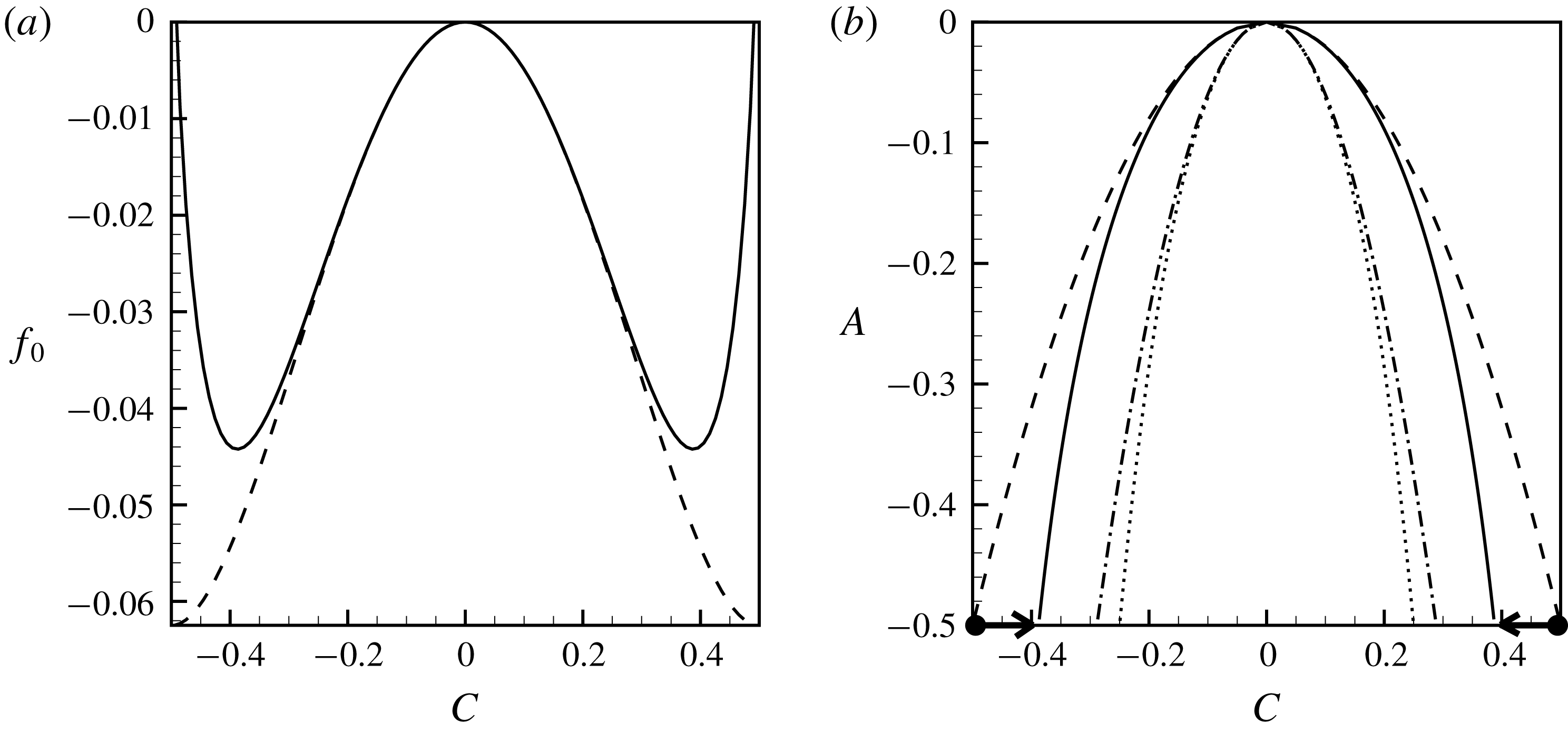
(a) The shapes of the free energy function (2.19), dashed line, and function (2.20), solid line, for $A=-1/2$ . (b) The phase diagrams of a binary mixture for function (2.19), dashed line, and function (2.20), solid line; and the shapes of the spinodal curves for function (2.19), dotted line, and function (2.20), dash-dotted line. The dots indicate the initial state of the mixture, and the arrows indicate the thermodynamic transformations experienced by a mixture.

The shapes of the functions (2.19) and (2.20) are depicted in figure 2(a), and the shapes of the phase diagrams that determine the equilibrium states of a mixture are depicted in figure 2(b). One sees that the non-dimensional parameter $A$ sets the value of the ‘mixture temperature’. The critical point is given by the ‘temperature’ $A=0$ and concentration $C=0$ . If the mixture temperature is above the critical point, $A>0$ , then the mixture is always homogeneous in equilibrium (or, liquids mix in any proportions), and if the mixture temperature is below the critical point, $A<0$ , then the mixture can be either homogeneous or heterogeneous in an equilibrium that is determined by the overall mass balance. One sees that two expressions (2.19) and (2.20) coincide near the critical point, and separate when $|C|\rightarrow 1/2$ . We wish to associate the values of concentration $1/2$ and $-1/2$ with two pure components of the mixture. The logarithmic terms of function (2.20) restrict the range of concentration to $[-1/2;1/2]$ , while function (2.19) allows overshootings (non-physical values of concentration that are either above $1/2$ or below $-1/2$ ). Function (2.20) is chosen for the current study, and the value of parameter $A$ is fixed at $-1/2$ . Figure 2(b) depicts the values of the initial concentrations in each phase, and the directions of the thermodynamic transformations that are experienced by a mixture. For $A=-1/2$ , the equilibrium states of a mixture are given by $\pm 0.388$ . A similar thermodynamic model was earlier used for modelling the dynamics of heterogeneous mixtures undergoing phase changes in other physical settings (see e.g. Vorobev & Boghi Reference Vorobev and Boghi2016; Xie & Vorobev Reference Xie and Vorobev2016; Vorobev & Khlebnikova Reference Vorobev and Khlebnikova2018; Lyubimova, Vorobev & Prokopev Reference Lyubimova, Vorobev and Prokopev2019).

The governing equations (2.14)–(2.18) include the following non-dimensional parameters,

(2.21a,b ) $$\begin{eqnarray}Sc=\frac{\unicode[STIX]{x1D702}_{\ast }}{\unicode[STIX]{x1D6FC}\unicode[STIX]{x1D707}_{\ast }},\quad Gs=\frac{\unicode[STIX]{x1D70C}_{\ast }^{2}\unicode[STIX]{x1D719}^{2}(a\unicode[STIX]{x1D714})^{2}L_{\ast }^{2}}{2\unicode[STIX]{x1D702}_{\ast }\unicode[STIX]{x1D6FC}\unicode[STIX]{x1D707}_{\ast }},\end{eqnarray}$$

(2.22a,b ) $$\begin{eqnarray}M=\frac{\unicode[STIX]{x1D702}_{\ast }^{2}}{\unicode[STIX]{x1D70C}_{\ast }^{2}\unicode[STIX]{x1D707}_{\ast }L_{\ast }^{2}},\quad Cn=\frac{\unicode[STIX]{x1D716}}{\unicode[STIX]{x1D707}_{\ast }L_{\ast }^{2}}.\end{eqnarray}$$

These parameters are defined by using the phenomenological constants introduced within the phase-field approach. The first two parameters are the phase-field analogues of the Schmidt and Gershuni numbers. Here, $\unicode[STIX]{x1D6FC}$ is the mobility coefficient, $\unicode[STIX]{x1D707}_{\ast }$ is a typical value of the chemical potential and the combination of $\unicode[STIX]{x1D6FC}\unicode[STIX]{x1D707}_{\ast }/\unicode[STIX]{x1D70C}_{\ast }$ plays the role of the diffusion coefficient. The phase-field equations are also characterised by two new parameters that we call the Mach number and the Cahn number (following Lowengrub & Truskinovsky (Reference Lowengrub and Truskinovsky1998)). The definition of the Mach number does not include the capillary constant, $\unicode[STIX]{x1D716}$ , however, this number sets the magnitude of the Korteweg force that determines the morphology of a liquid/liquid interface. Higher Mach numbers would obviously correspond to weaker surface tension forces (making the results similar to the classical approach when the surface tension forces are disregarded), and smaller Mach numbers would correspond to the stronger interfacial stresses. The Cahn number also determines the role of the surface tension forces, as it is proportional to the capillary constant $\unicode[STIX]{x1D716}$ . The Cahn number also sets the thickness of the transitional layer between the phases, that can be estimated as $\sqrt{-Cn/A}$ (see e.g. Lowengrub & Truskinovsky Reference Lowengrub and Truskinovsky1998). The other parameter of the phase-field approach is the ‘mixture temperature’ $A$ .

The governing equations are supplemented with the boundary conditions. We impose the no-slip condition for the average velocity and the no-penetration condition for the pulsational flow,

(2.23a,b ) $$\begin{eqnarray}\boldsymbol{u}=0,\quad w_{n}=0.\end{eqnarray}$$

We also impose the absence of the diffusive flux at the container’s walls. Since the diffusive flux is determined by the gradient of the chemical potential, this boundary condition reads,

(2.24) $$\begin{eqnarray}\frac{\unicode[STIX]{x2202}\unicode[STIX]{x1D707}}{\unicode[STIX]{x2202}n}=0.\end{eqnarray}$$

Here $\boldsymbol{n}$ is a unit vector normal to the wall. In comparison with the classical equations, the phase-field equations are of the higher (forth) order in terms of the concentration field, and because of this they require one additional boundary condition that would reflect the wetting properties of the walls. In the current work, we use this boundary condition in its simplest form,

(2.25) $$\begin{eqnarray}\frac{\unicode[STIX]{x2202}C}{\unicode[STIX]{x2202}n}=0.\end{eqnarray}$$

This condition assumes that the molecules of the wall interact with the molecules of the mixture components equally (in other words, the contact line is orthogonal to the interface).

The governing equations (2.14)–(2.18) written in terms of the vorticity–streamfunction read,

(2.26) $$\begin{eqnarray}\frac{\unicode[STIX]{x2202}\unicode[STIX]{x1D6FA}}{\unicode[STIX]{x2202}t}+J(\unicode[STIX]{x1D6FA},\unicode[STIX]{x1D713})=\unicode[STIX]{x1D6FB}^{2}\unicode[STIX]{x1D6FA}+\frac{1}{M}J(\unicode[STIX]{x1D707},C)+\frac{Gs}{Sc}J\left(C,\frac{\unicode[STIX]{x2202}\unicode[STIX]{x1D6F7}}{\unicode[STIX]{x2202}x}\right),\end{eqnarray}$$

(2.27) $$\begin{eqnarray}\frac{\unicode[STIX]{x2202}C}{\unicode[STIX]{x2202}t}+J(C,\unicode[STIX]{x1D713})=\frac{1}{Sc}\unicode[STIX]{x1D6FB}^{2}\unicode[STIX]{x1D707},\end{eqnarray}$$

(2.28a,b ) $$\begin{eqnarray}\unicode[STIX]{x1D6FB}^{2}\unicode[STIX]{x1D713}=-\unicode[STIX]{x1D6FA},\quad \unicode[STIX]{x1D6FB}^{2}\unicode[STIX]{x1D6F7}=\frac{\unicode[STIX]{x2202}C}{\unicode[STIX]{x2202}x},\end{eqnarray}$$

(2.29) $$\begin{eqnarray}\unicode[STIX]{x1D707}=\frac{3}{4}\ln \left(\frac{1/2+C}{1/2-C}\right)-(3-2A)C-Cn\unicode[STIX]{x1D6FB}^{2}C.\end{eqnarray}$$

And the boundary conditions read

(2.30a-d ) $$\begin{eqnarray}\unicode[STIX]{x1D713}=0,\quad \frac{\unicode[STIX]{x2202}\unicode[STIX]{x1D713}}{\unicode[STIX]{x2202}n}=0,\quad \frac{\unicode[STIX]{x2202}\unicode[STIX]{x1D6F7}}{\unicode[STIX]{x2202}n}=Cw_{0n},\quad \frac{\unicode[STIX]{x2202}\unicode[STIX]{x1D707}}{\unicode[STIX]{x2202}n}=\frac{\unicode[STIX]{x2202}C}{\unicode[STIX]{x2202}n}=0.\end{eqnarray}$$

Finally, the initial state of the system is set by the following concentration field,

(2.31) $$\begin{eqnarray}C_{0}=0.495\tanh \left(\frac{y-1/2}{\unicode[STIX]{x1D6FF}_{0}}\right).\end{eqnarray}$$

Here, the initial interface thickness is (almost always) set by expression, $\unicode[STIX]{x1D6FF}_{0}=\sqrt{-Cn/A}$ , excepting figure 4 where the interfacial thickness is treated as an additional independent parameter. There is no average motion at the initial time moment ( $\boldsymbol{u}_{0}=0$ ). (To simplify comparisons with other studies, we show the numerical results for the interface that is horizontal (stretches along the larger dimension of the container) in the initial moment as set in experiment (Gaponenko et al. Reference Gaponenko, Torregrosa, Yasnou, Mialdun and Shevtsova2015b ). Under weightlessness conditions the initial shape of the interface may be different, and we also performed the simulations when the interface was curved at the initial moment, but no principal differences in the results were obtained.)

2.3 Numerical solution. Convergence

The mathematical problems set for the classical and phase-field models are solved numerically in the vorticity–streamfunction formulation using the finite-difference approach. An explicit numerical scheme that uses the first-order discretisation for the time derivative and the second-order discretisation for the spatial derivatives is used.

To trace the intensity of the fluid motion and the intensity of the molecular mixing the following integral parameters are calculated.

1. (i) The total kinetic energy of the average fluid motion,

   (2.32) $$\begin{eqnarray}E_{k}=\frac{1}{2}\int _{V}u^{2}\,\text{d}V,\end{eqnarray}$$
   where $V$ is the total volume of the fluid domain (in two dimensions, the volume is in fact replaced by an area of a fluid domain in the $x$ – $y$ plane). This is the non-dimensional expression, and the units of energy that were used for non-dimensionalisation are $\unicode[STIX]{x1D70C}_{\ast }u_{\ast }^{2}L_{\ast }^{2}$ .

2. (ii) The kinetic energy of the pulsational motion,

   (2.33) $$\begin{eqnarray}E_{w}=\frac{Gs}{2Sc}\int _{V}w^{2}\,\text{d}V.\end{eqnarray}$$

3. (iii) The interfacial energy,

   (2.34) $$\begin{eqnarray}E_{i}=\frac{Cn}{M}\int _{V}(\unicode[STIX]{x1D735}C)^{2}\,\text{d}V.\end{eqnarray}$$

4. (iv) The volume of the transitional layer between the phases, that is calculated as the volume of the fluid domain with the concentration values in the range $|C|\leqslant 0.2$ .

5. (v) The average concentration in each liquid phase. It is assumed that the position of the interface is given by the value $C=0$ . Liquid $1$ is determined by the negative values of the concentration field, and liquid $2$ is determined by the positive values of the field of concentration. The average concentration in liquid $1$ is denoted by $C_{1}$ , and the average concentration in liquid $2$ is denoted by $C_{2}$ (owing to the symmetry of the examined problem (the symmetry of the initial state and the symmetry of the phase diagram, figure 2 b) in all calculations $C_{1}=-C_{2}$ .).

Figure 3.

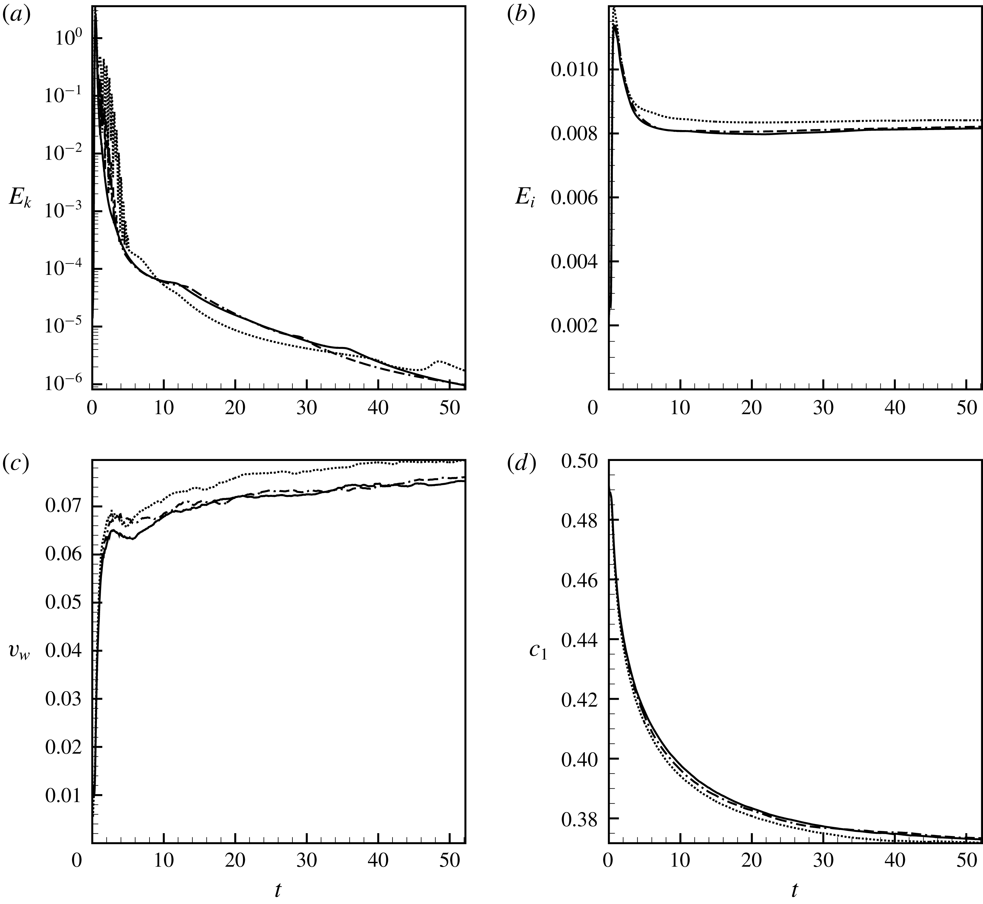
(a) The total kinetic energy of the average motion, (b) the interfacial energy, (c) the volume of the interface and (d) the average concentration in one liquid versus time. The results are shown for $A=-0.5$ , $Sc=10^{4}$ , $Gs=5\times 10^{6}$ , $M=1$ and $Cn=2.5\times 10^{-5}$ . The dotted lines show the data obtained with $400\times 800$ grid points, the dashed lines are for $500\times 1000$ grid points and the solid lines are for $600\times 1200$ grid points, respectively.

The numerical convergence and the mesh independence of the numerical simulations are illustrated by figure 3. The required resolution is determined by the governing parameters: the better resolution is needed at greater values of the Schmidt and Gershuni numbers, which should be explained by smaller diffusive length scales and higher flow intensities, and also at smaller values of the Cahn number that correspond to smaller thicknesses of interfaces. In figure 3, one may see that the lines that depict the time changes of different quantities clearly converge to the limiting curves.

Figure 4.

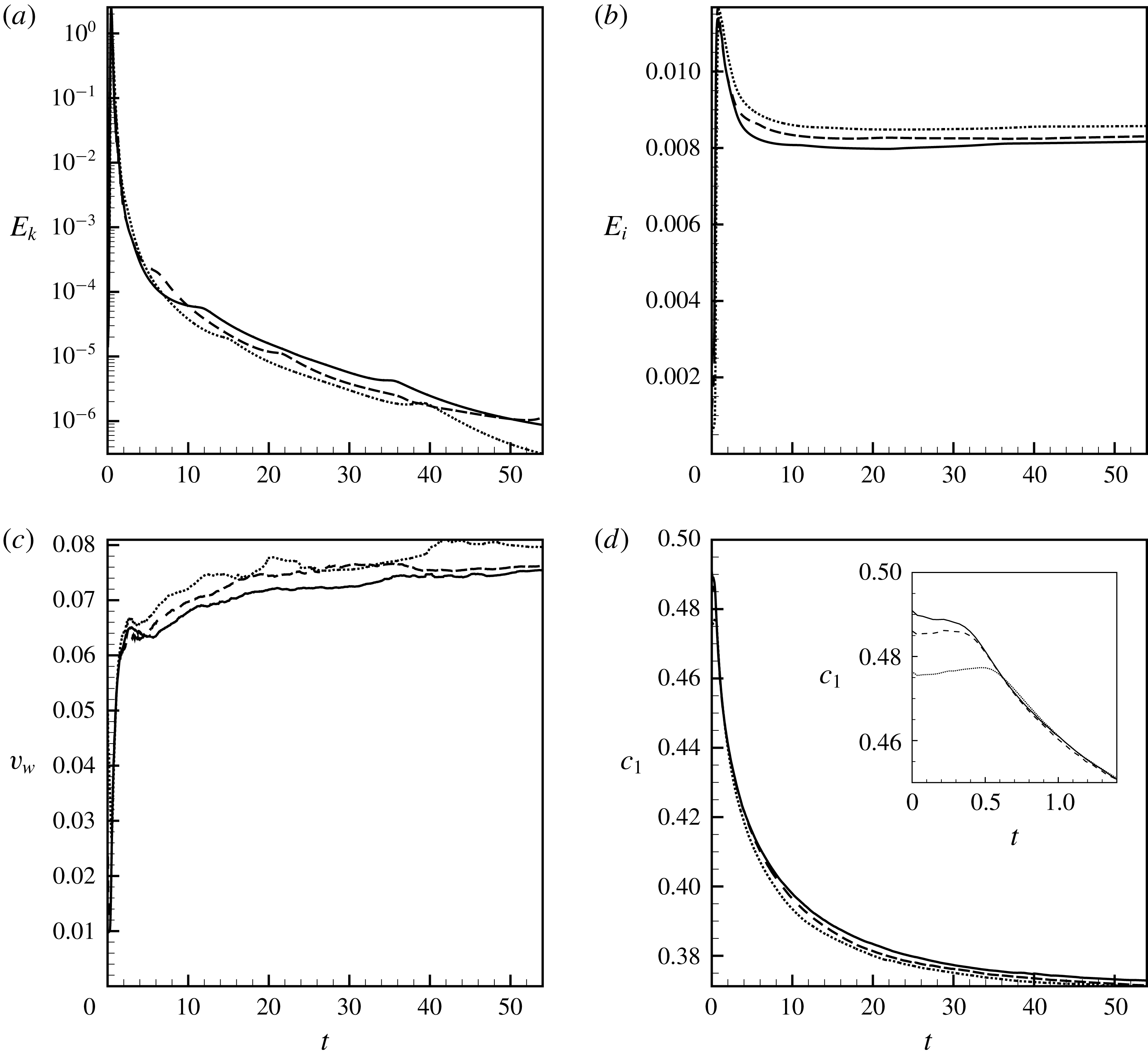
(a) The total kinetic energy of the average motion, (b) the interfacial energy, (c) the volume of the interface and (d) the average concentration in one liquid versus time. The results are shown for $A=-0.5$ , $Sc=10^{4}$ , $Gs=5\times 10^{6}$ , $M=1$ and $Cn=2.5\times 10^{-5}$ , and for different initial thicknesses of the interface, the solid lines shows the data for $\unicode[STIX]{x1D6FF}_{0}=\sqrt{-Ca/A}\approx 0.007$ , the dashed lines are for $\unicode[STIX]{x1D6FF}_{0}\approx 0.014$ and the dotted lines are for $\unicode[STIX]{x1D6FF}_{0}\approx 0.028$ .

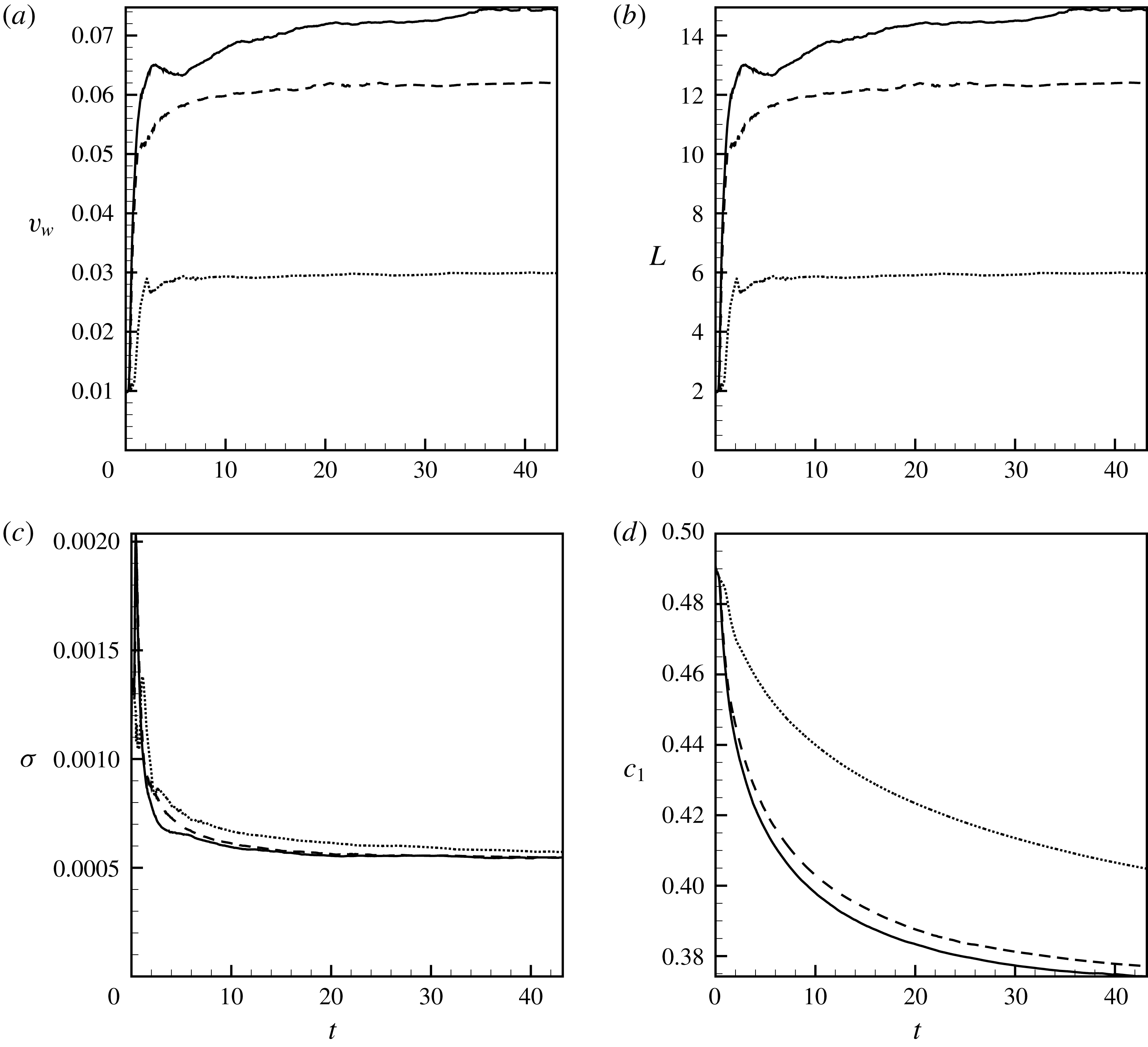
For the phase-field simulations, it is also important to investigate the convergence of the numerical results when values of the interface thickness gradually decrease. The thickness of a real interface between two immiscible liquids is of the order of several molecular layers, which is equivalent to zero value for the hydrodynamic (macroscopic) approach. The interface is represented by a transitional layer of a finite thickness for the sake of numerical simulations, and these interface thicknesses are not equal to the real thicknesses of interfaces. One however needs to show that the numerical results converge when the thickness of the interface tends to zero (tends to the real thickness). It should be mentioned that there are some cases, e.g. the interface of a near critical mixture, or the interface between two liquids miscible in all proportions after a prolonged contact, when the interfacial boundary could be quite diffusive, and in those cases both the numerical and physical thicknesses of the interfacial boundary are both finite and hence the simulations can be fulfilled with the use of the real thickness of the interface. Figure 4 depicts the data obtained for the different values of the initial thicknesses of interfaces, $\unicode[STIX]{x1D6FF}_{0}$ . The curves may be different in the very initial moments (see e.g. the insert in figure 4 d), but they quickly converge to a single curve. Further, the curves slowly diverge from each other, nevertheless, they stay sufficiently close to claim that our numerical results are virtually independent of the value of $\unicode[STIX]{x1D6FF}_{0}$ .

Figure 5.

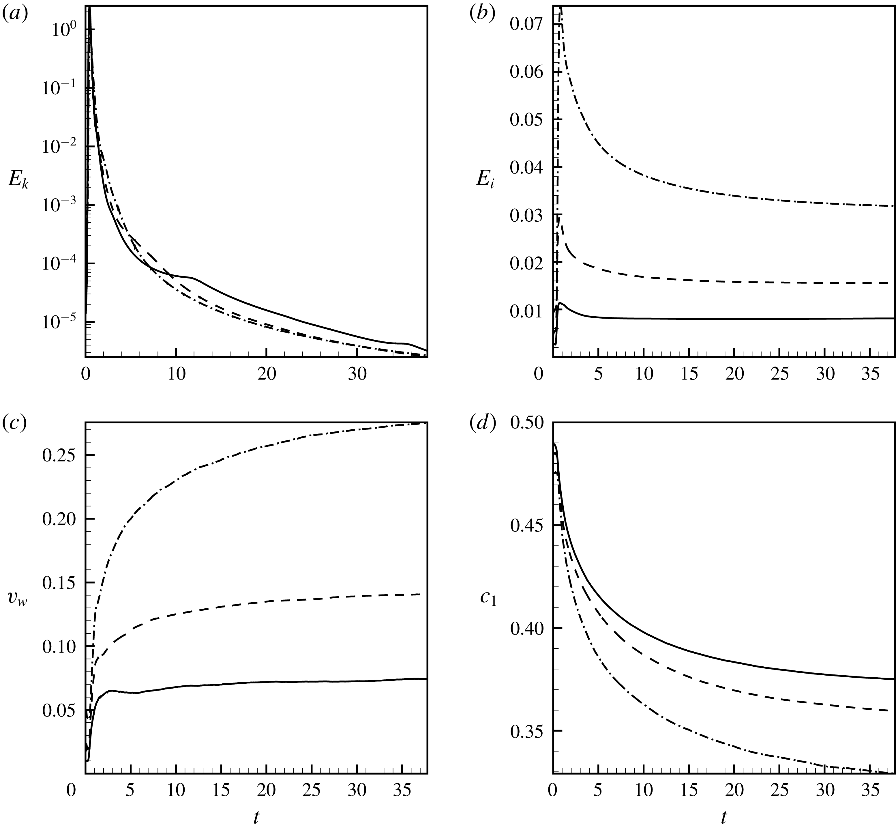
(a) The total kinetic energy of the average motion, (b) the interfacial energy, (c) the volume of the interface and (d) the average concentration in one liquid versus time. The results are shown for $A=-0.5$ , $Sc=10^{4}$ , $Gs=5\times 10^{6}$ , $M=1$ and $Cn=2.5\times 10^{-5}$ (solid lines), $Cn=10^{-4}$ (dashed lines) and $Cn=4\times 10^{-4}$ (dash-dotted lines).

Figure 6.

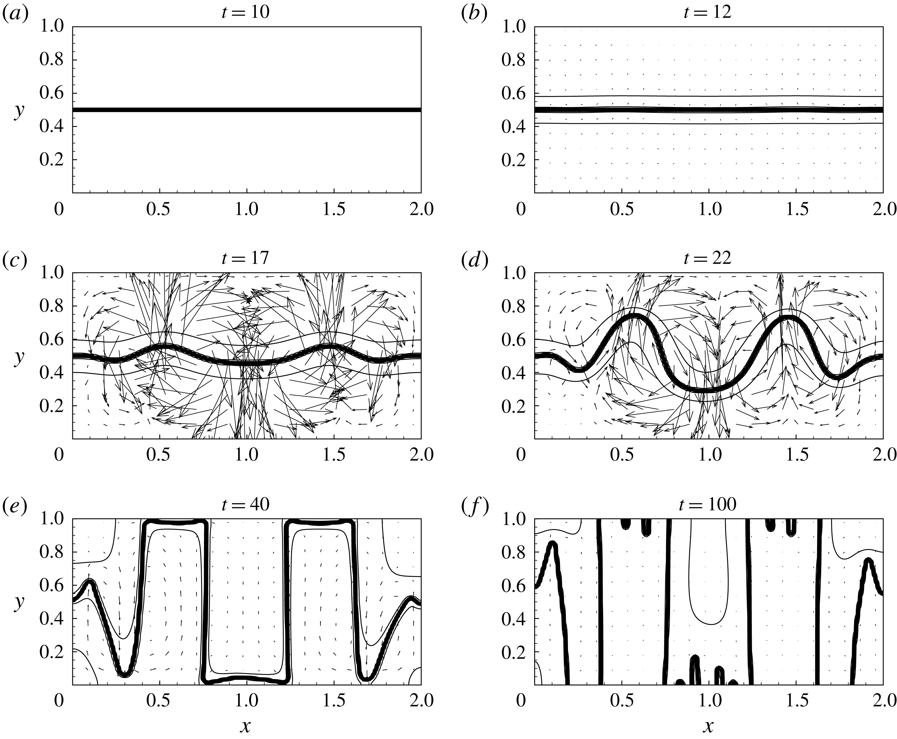
Snapshots of the fields of concentration (isolines) and velocity (vectors). The data are obtained for the run fulfilled with the use of the classical model for $Sc=10^{4}$ and $Gs=10^{5}$ . The double-arrow line in (a) shows the direction of vibration.

Some of the curves in figure 4 are plotted by taking an initial thickness of the interface different from the equilibrium value, $\sqrt{-Cn/A}$ . Since the initial state of a mixture differs from the state of thermodynamic equilibrium, the initial thickness of the interface (similar to the levels of concentrations in the neighbouring liquids) should in general be different from its equilibrium value. We however observe that all curves quickly converge to a single curve that is obtained when the initial interface thickness is taken equal to its equilibrium value. At this moment the whole binary mixture does not reach the state of thermodynamic equilibrium yet, and there is ongoing diffusive mass transport across the liquid/liquid boundary, although, the adjustment of the interface thickness to its equilibrium value is already completed.

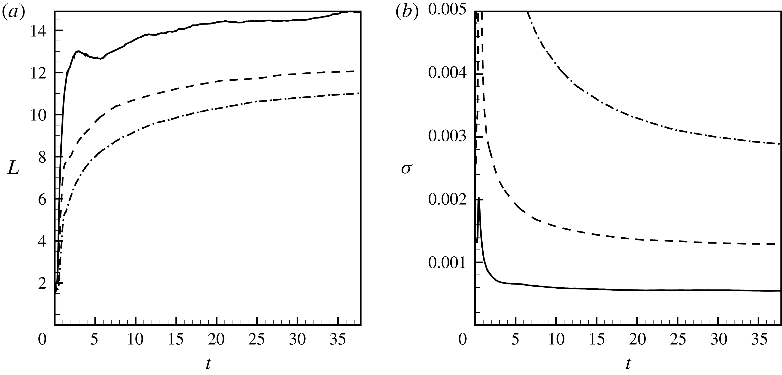
In figure 5, we investigate the numerical convergence on the interface thickness for the three runs that are fulfilled with the different values of the Cahn number. By altering the Cahn number we simultaneously change the interface thickness and the surface tension coefficient that is associated with the interface. The difference in the values of the interfacial energy is explained by a factor $Cn$ that appears in front of expression (2.34), so the curves for the quantity, $E_{i}/Cn$ , would lie much closer to each other. The curves of the volume of the interfacial line also differ by a similar factor (one sees that when $Cn$ is doubled the volume of the interfacial line is also doubled). The curves in figure 5(a,d) demonstrate a clear convergence of the numerical results upon a gradual decrease in the values of the interfacial thickness (the distance between the curves gradually decreases when the Cahn number is taken smaller and smaller).

In conclusion, we say that the results shown in the next section of our work are obtained with the numerical grids that contain at least $450\times 900$ grid nodes (for lower Gershuni numbers) and typically include $600\times 1200$ grid nodes (for the runs fulfilled for higher Gershuni numbers). For the phase-field simulations, the main results are obtained for the fixed value of the Cahn number, $Cn=2.5\times 10^{-5}$ , fixed value of parameter $A$ , $A=-1/2$ , and for the initial interface thickness, $\unicode[STIX]{x1D6FF}_{0}=\sqrt{-Cn/A}\approx 0.007$ .

3.1 Classical approach

We present the numerical results starting from the data obtained with the use of the classical equations (2.1)–(2.3). Similar data (for a slightly more general model that takes into account the concentration dependencies of the diffusion and viscosity coefficients) were earlier reported in the works by Gaponenko et al. (Reference Gaponenko, Torregrosa, Yasnou, Mialdun and Shevtsova2015b ).

Gaponenko et al. (Reference Gaponenko, Torregrosa, Yasnou, Mialdun and Shevtsova2015b ) presented the results in the dimensional form, and we present our data using the non-dimensional variables. The data sets can still be easily compared as all parameters that are used for our simulations were taken to be close to the experimental values. In particular, the experiment deals with mixtures of $90\,\%$ water– $10\,\%$ isopropanol and $50\,\%$ water– $50\,\%$ isopropanol. Owing to the dependence of the viscous and diffusion coefficients on mixture composition, it is difficult to set single values of the Schmidt and Gershuni numbers that would work for the entire fluid domain. Depending on a particular location within the container, the Schmidt number may vary in the range of 2030–21 165. The range of the Gershuni numbers (for different levels of vibrations, and for different locations in the cavity) could be roughly estimated in the range of $10^{4}$ – $10^{9}$ (the upper end of this range corresponds to rather large amplitudes of vibration that are even greater than the size of the container). Gaponenko et al. (Reference Gaponenko, Torregrosa, Yasnou, Mialdun and Shevtsova2015b ) avoided this problem by solving the equations in the dimensional form and by taking into account the density dependencies of the phenomenological parameters. We neglect the concentration dependencies of the viscosity and diffusivity, and characterise the mixture by a single Schmidt number (which we set $Sc=10^{4}$ for all calculations) and by a single Gershuni number (for a fixed level of the vibrational forcing). In the phase-field theory, that is considered later, the concentration dependence of the diffusion coefficient is given by free energy function (2.20), namely ${\sim}\text{d}^{2}f_{0}/\text{d}C^{2}$ , however, in the classical approach the diffusion coefficient is assumed to be just constant. Finally, we mention that the real convective time scale varies in the range of (16.6–39.08) s. The convective time scale is used as a unit of the non-dimensional time in our work, and thus, we may roughly say that one unit of the non-dimensional time is approximately 30 s.

Figure 7.

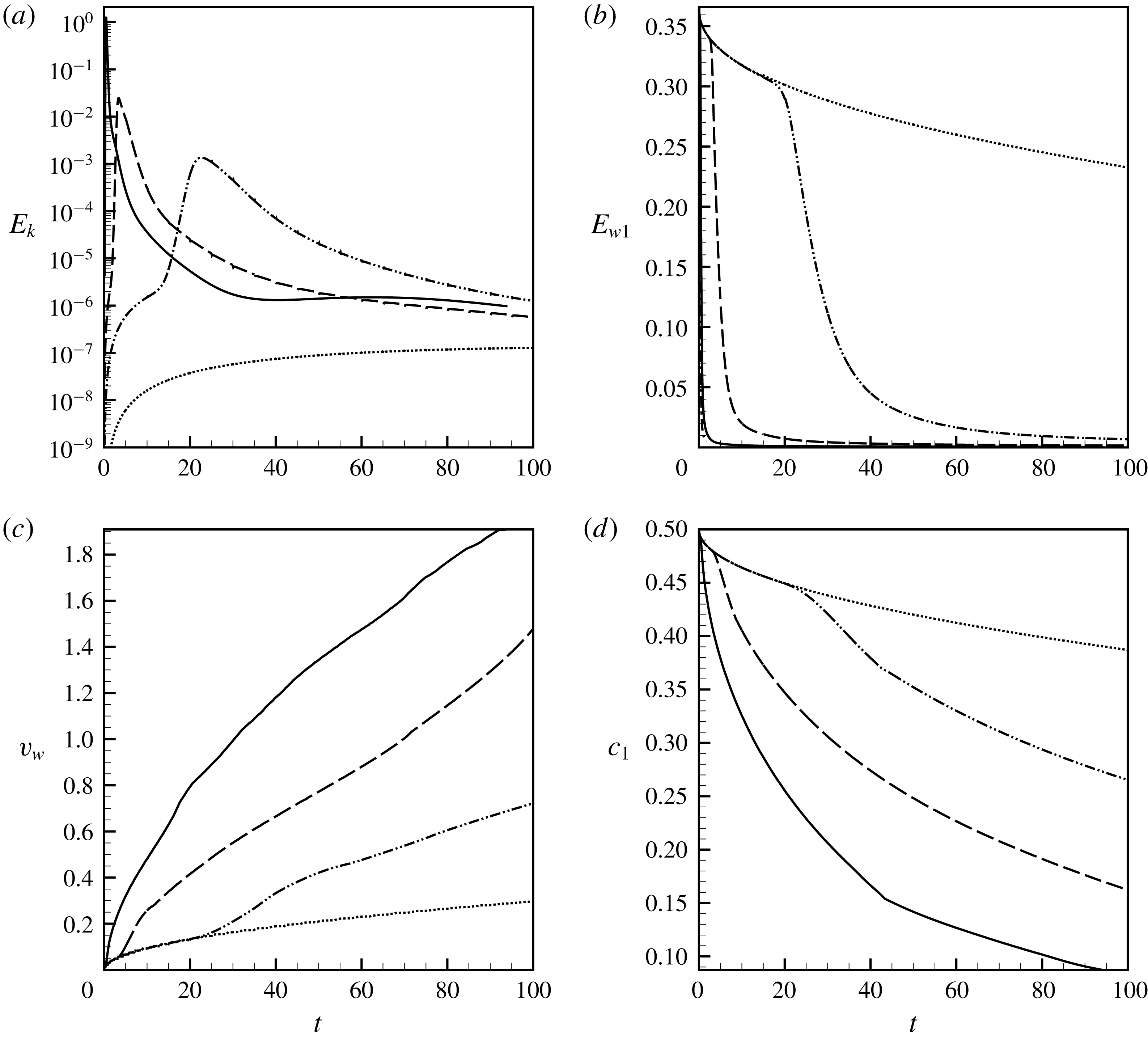
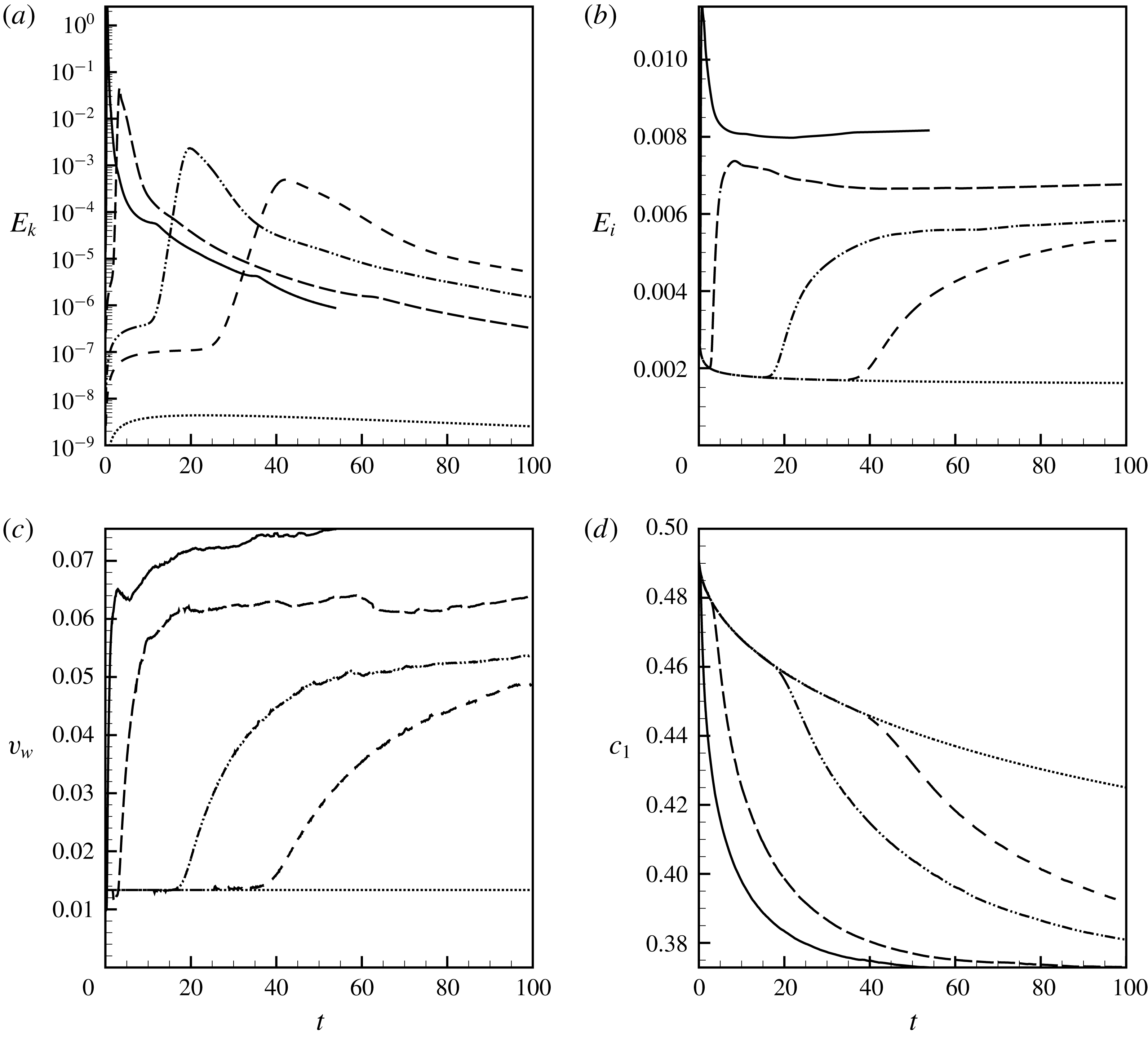
(a) The kinetic energy of the average flow, (b) the kinetic energy of the pulsation flow (here $E_{w1}\equiv E_{w}Sc/Gs$ ), (c) the volume of the interface and (d) the average concentration in liquid $1$ versus time. The data are obtained for the run fulfilled with the use of the classical model for $Sc=10^{4}$ and $Gs=10^{4}$ (dotted line), $Gs=10^{5}$ (dash-dot-dotted line), $Gs=5\times 10^{5}$ (dashed line) and $Gs=5\times 10^{6}$ (solid line).

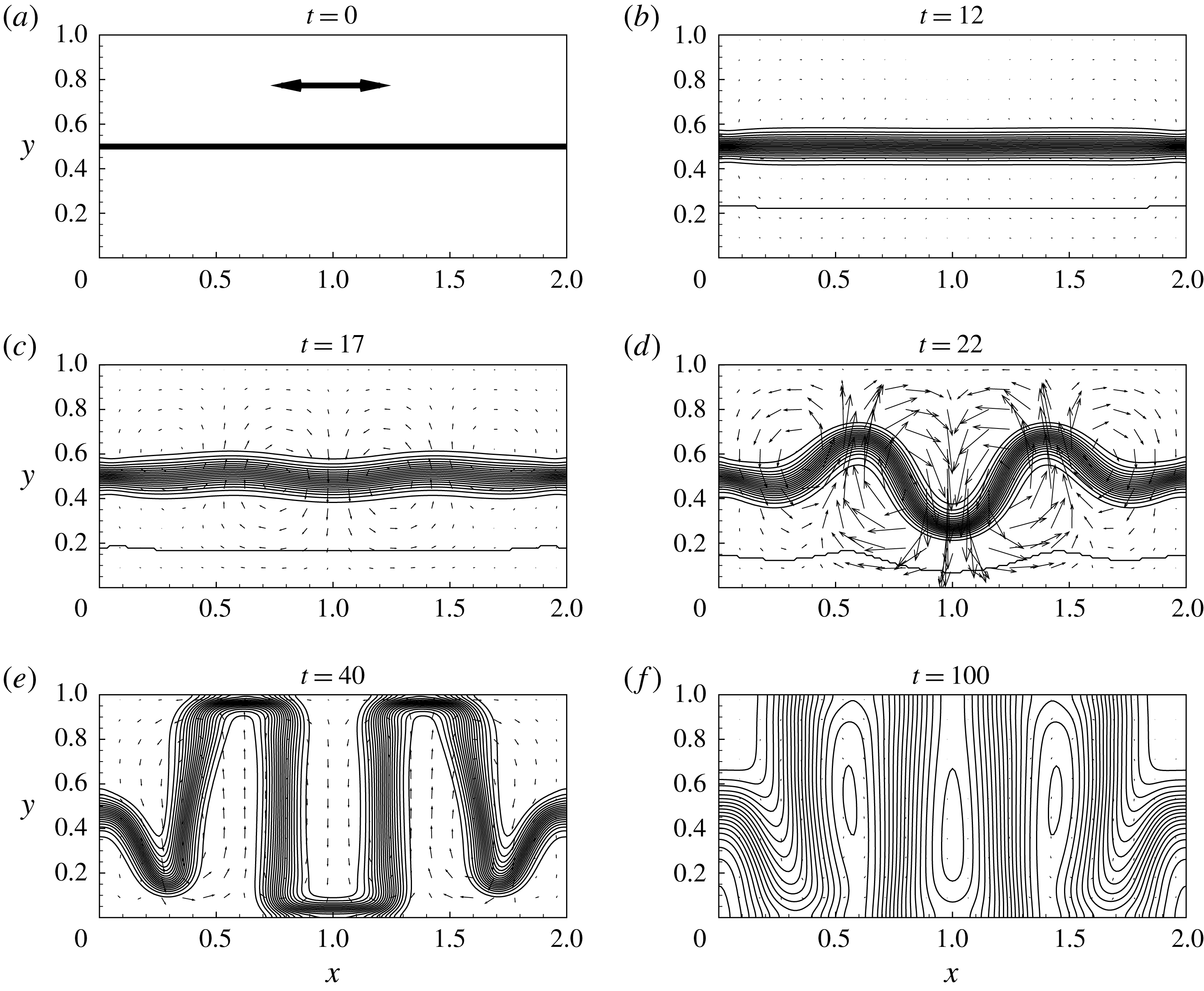
The data shown in figures 6 and 7 present typical evolutions of an interface in a binary system that is subjected to high-frequency vibrations of different intensities. The snapshots shown in figure 6 demonstrate a good general agreement of the numerical results with the experimental observations reported by Gaponenko et al. (Reference Gaponenko, Torregrosa, Yasnou, Mialdun and Shevtsova2015b ). In the beginning, the vibrations induce some weak average flows in both fluid domains. The magnitude of the induced flow grows in time, but when the vibrational forcing is weak (lower Gershuni numbers), during the numerical run the induced flows remain too weak to disturb the interface shape: the interface remains flat and it just slowly smears in time. If however the vibrational forcing is stronger, the average motion induced by the vibrations destabilises the flat interface, eventually forming a pillar-shaped structure in a container. The vertical growth of the pillars is restricted by the container’s height, and when the pillars reach the upper and lower walls of the cavity (occupy the full height of the cavity), the intensity of the average and pulsation motions decay. The further development of the pillars occurs much slower, and it is characterised by slow diffusive smearing of immovable pillar’s walls. These pillar-shaped structures represent a phenomenon of a frozen relief (or frozen waves).

In figure 6(f), that corresponds to the time moment of $100$ (about an hour in physical time), the interface is very diffuse. The experimental results (see Gaponenko et al. Reference Gaponenko, Torregrosa, Yasnou, Mialdun and Shevtsova2015a ,Reference Gaponenko, Torregrosa, Yasnou, Mialdun and Shevtsova b ; Shevtsova et al. Reference Shevtsova, Gaponenko, Yasnou, Mialdun and Nepomnyashchy2015, Reference Shevtsova, Gaponenko, Yasnou, Mialdun and Nepomnyashchy2016) do not include the pictures with such diffusive interfacial boundaries, which may be explained by a difficulty of processing similar images or by time restrictions of parabolic flights that were used to achieve the weightlessness conditions. It is also interesting to note that a typical diffusive time scale is of the order of $Sc$ , and hence one expects a noticeable diffusive smearing over a time period of the order of $10^{4}$ . Figure 6(f) clearly shows that the diffusive smearing is substantially sped up by the vibrational forcing, so the liquids become nearly indistinguishable after a time period of $100$ , even under the action of relatively moderate vibrations ( $Gs=10^{5}$ ). Figure 6(f) also answers Wolf’s question (Wolf Reference Wolf2018) on the long-term stability of the frozen waves: one sees that the frozen waves formed on a miscible interface remain stable at least until the interfacial boundary can be visually identified.

Figure 7(a) shows the time changes of the total kinetic energy of the average flow for the different Gershuni numbers. At $Gs=10^{4}$ the intensity of the induced average flow grows with time, however, at least for the duration of the numerical run, the flow remains too weak to affect the interface shape. At $Gs\geqslant 4\times 10^{4}$ , at some moment the slower growth of the kinetic energy is suddenly replaced by a faster growth. This happens at the moment of the interface reconstruction that eventually results in the formation of several ‘frozen’ pillars stretched from the bottom to the top wall of the container. When the pillars are fully set the intensity of the fluid motion drops to almost zero. Figure 7(b) depicts the time changes of the kinetic energy of the pulsation flow. The pulsation flow has the highest intensity in the beginning of the numerical run when the liquid/liquid interface is sharp, and the initial diffusive smearing of the interface slowly decreases the pulsation motion. At the moment of interface reconstruction, the intensity of the pulsation flow rapidly decays. Figure 7(c) shows how the volume of the interfacial zone grows with time. Again, the rapid increase of the volume corresponds to the interface reconstruction. Figure 7(d) shows the time changes of the average concentrations in one of the liquids. The reconstruction of the interface increases the molecular mixing that is to be explained by the growth of the interface length (i.e. the contact area of two liquids).

Figure 8.

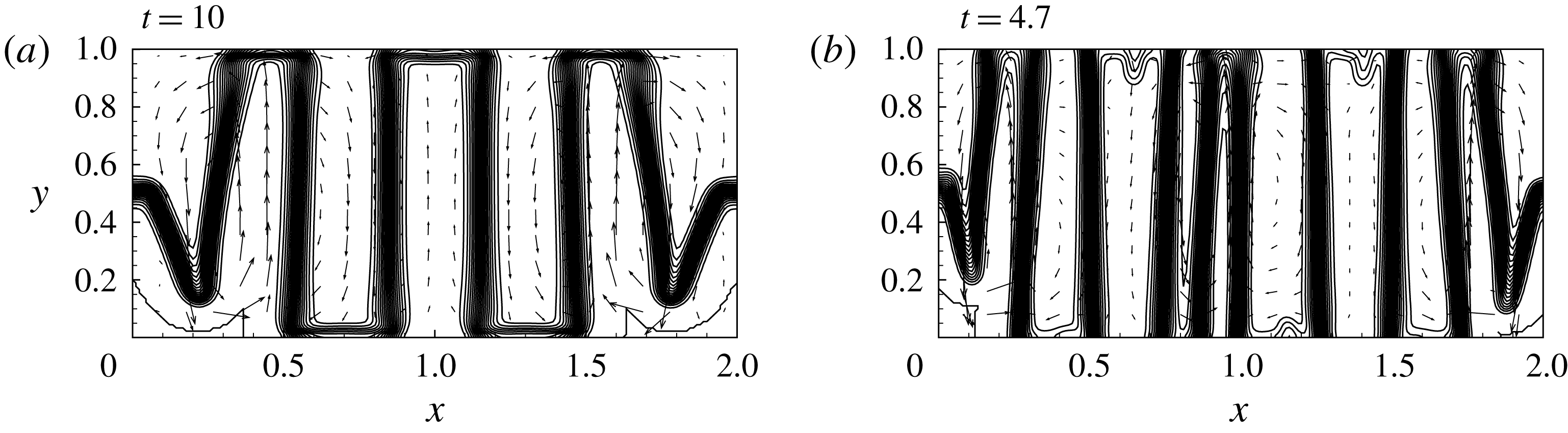
The shape of an interface subjected to the vibrations with $Gs=5\times 10^{5}$ (a) and $Gs=5\times 10^{6}$ (b). The data are obtained for the classical model, for $Sc=10^{4}$ .

In figure 7 one notices that while the interface is flat the dynamics of the binary mixture is solely determined by the diffusive process. In the later moments, when the frozen pillars are fully set, the hydrodynamic motion in the container is also absent, and the evolution of a mixture is again determined by diffusion. Nevertheless, there are clear differences between the initial and later dynamics of the mixture: the initial dynamics is independent of vibrations, and the later dynamics occurs differently for the vibrations of different intensities. This needs to be explained by the dependence of the shape of the frozen relief (the different number of the pillars in the container) on the Gershuni number. The greater the level of vibrations is, the more pillars are formed in the container, as seen in figure 8. The liquid/liquid contact surface is obviously greater when there are more pillars, which explains the differences in the rates of molecular diffusion at the later time periods.

Figure 9.

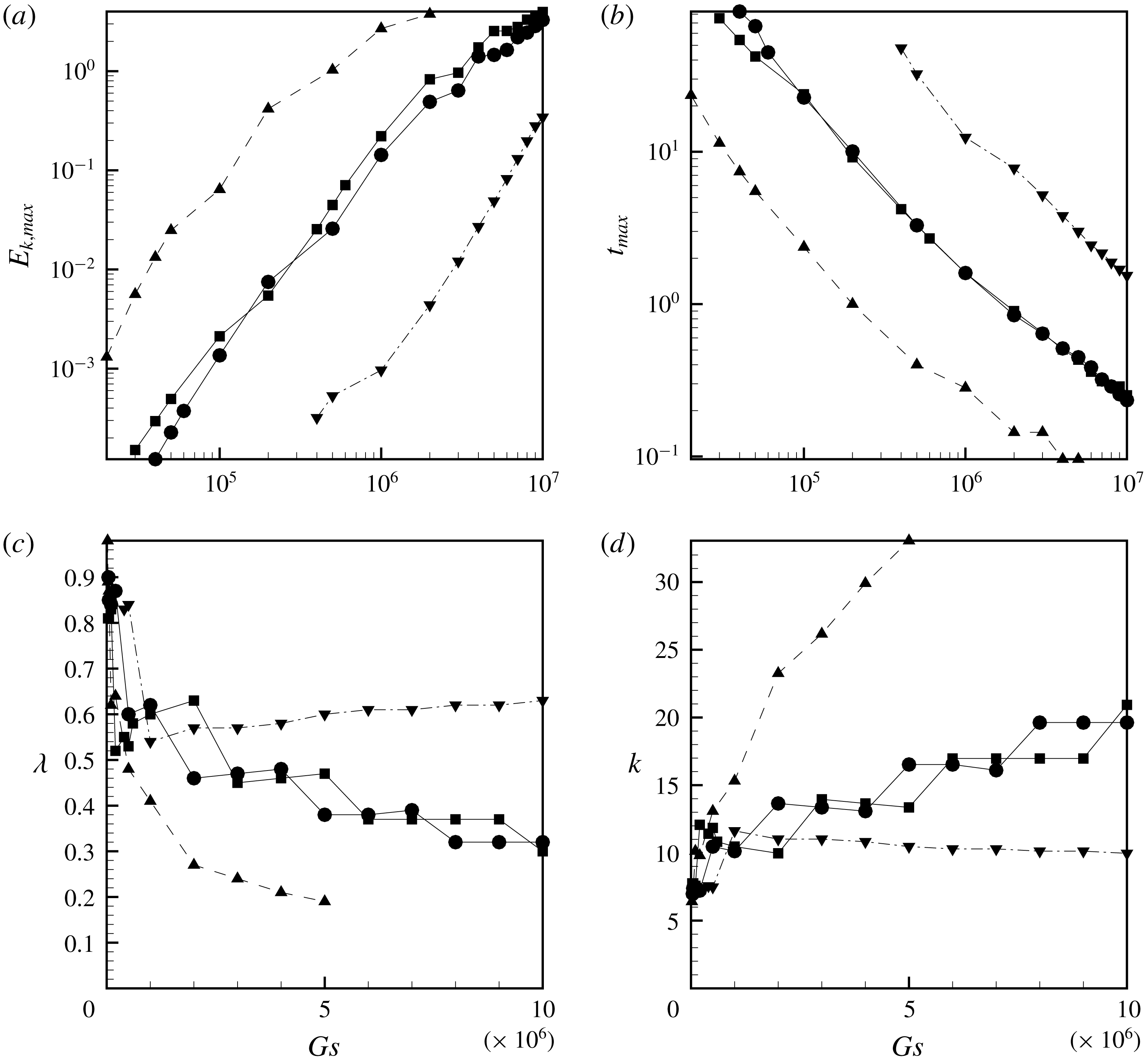
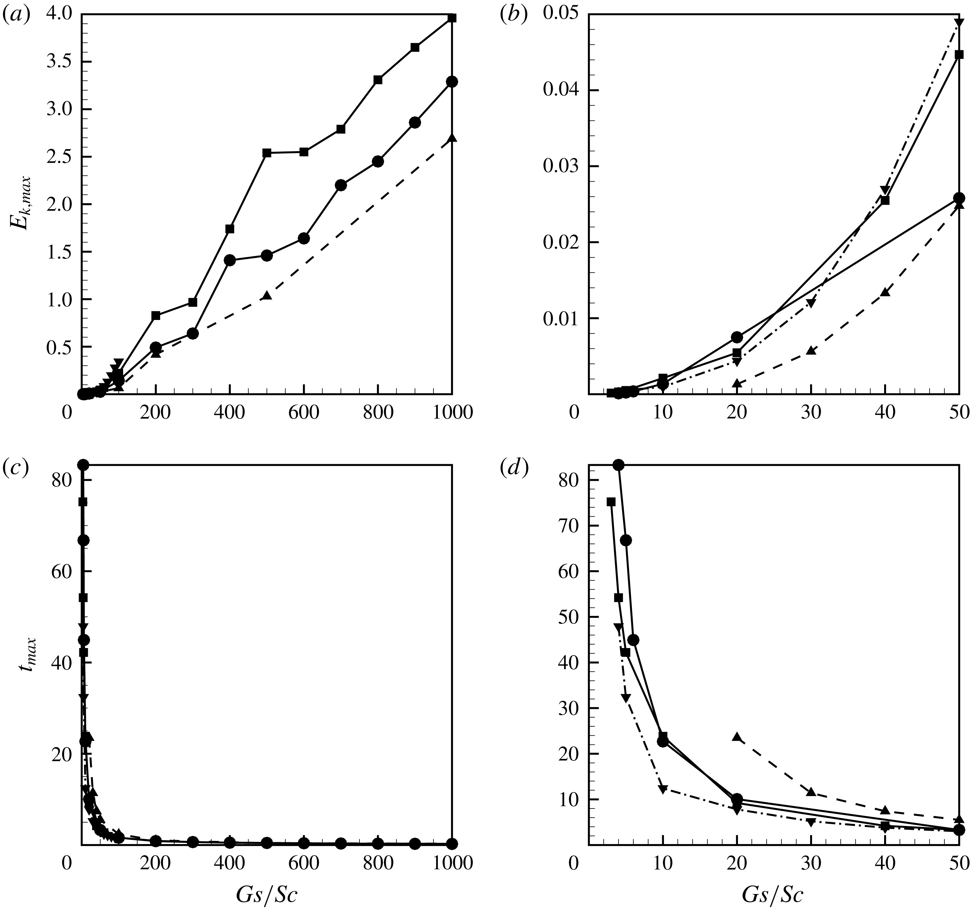
(a,b) The maximum value of the kinetic energy of the average flow during the evolution of a binary mixture and the time moments when the kinetic energy is maximum versus the Gershuni number. (c,d) The wavelengths and the wavenumbers that characterise the periodicity of the frozen pillars in the horizontal dimension versus the Gershuni number. The data are obtained for the classical model (‘circles’ for $Sc=10^{4}$ , ‘triangles’ for $Sc=10^{3}$ and ‘nablas’ for $Sc=10^{5}$ ) and for the phase-field simulations (‘squares’ for $Sc=10^{4}$ , $M=1$ , $Cn=2.5\times 10^{-5}$ and $A=-0.5$ ).

In figure 7 one sees that the reconstruction of an interface starts earlier, occurs faster and the maximum values of the kinetic energy are greater for the runs with higher Gershuni numbers, which is also illustrated in figures 9(a,b). In figure 9(c,d) the horizontal size of the pillars characterised by a wavelength that is calculated by taking the ratio of the numbers of several fully formed pillars (two pillars form a ‘wave’) in a central part of the container over the width of the region occupied by these pillars.

Figure 10.

The maximum value of the kinetic energy of the average flow during the evolution of a binary mixture (a,b) and the time moments when the kinetic energy is maximum (c,d) versus $Gs/Sc$ (the ratio of Gershuni and Schmidt numbers). The data are obtained for the classical model (‘circles’ for $Sc=10^{4}$ , ‘triangles’ for $Sc=10^{3}$ and ‘nablas’ for $Sc=10^{5}$ ) and for the phase-field simulations (‘squares’ for $Sc=10^{4}$ ,  $M=1$ , $Cn=2.5\times 10^{-5}$ and $A=-0.5$ ).

Particular attention in the current work is paid to the question of whether the formation of the frozen waves requires vibrational forcing with an intensity over a certain threshold level. In the classical theory (2.1)–(2.3), the surface tension is completely disregarded. In accordance with (1.1) under weightlessness conditions the appearance of the frozen waves may happen in the presence of high-frequency vibrations of any intensity, which could be easily understood from the analysis of (2.1)–(2.3) where the vibrational force is the only term capable of setting the interfacial shape. In our calculations (for $Sc=10^{4}$ ) the minimum Gershuni number that allows the formation of the frozen relief is $Gs_{c}=4\times 10^{4}$ , and as one sees in figure 7 the interface remains flat for $Gs=10^{4}$ for the duration of the numerical run, i.e. for $t<100$ .

The simulations fulfilled for the different levels of the Schmidt number reveal a strong influence of this parameter, which however can be easily explained by the fact that the amplitude of the vibrational force in (2.1) is set by the ratio $Gs/Sc$ . Figure 10 shows the dependencies of the maximum value of the kinetic energy during the reconstruction of the interface and the time moment when the kinetic energy reaches the maximum value as functions of the ratio $Gs/Sc$ . In the new coordinates the curves obtained for different Schmidt numbers almost coincide when $(Gs/Sc)\rightarrow 0$ . In addition, one sees that when $(Gs/Sc)\rightarrow 0$ the time required for the formation of the waves increases exponentially. When the time needed for the reconstruction of an interface becomes too long, the interface gets too diffusive (practically indistinguishable) before hydrodynamic motion has time to reshape the interface. Moreover, the interface smearing reduces the magnitude of the vibrational forcing even further, making its influence even less significant over the time. In this case the isolines of the concentration field become only slightly distorted by the hydrodynamic motion, so that the formation of the frozen waves cannot be seen. We observe such a behaviour for $(Gs/Sc)\leqslant 4$ .

In figure 9(c) one sees that the longest structures that are formed in the container have a wavelength of approximately $0.85$ (for $Gs=5\times 10^{5}$ and $Sc=10^{4}$ ), which corresponds to three pillars (see figure 6 e). When the Gershuni number is increased the number of pillars that are formed in the container also grows. Although, as can be seen from figure 9(c,d), the growth in the number of the pillars does not happen smoothly: there is a sequence of critical Gershuni numbers when two new pillars (one wave) are added that also makes the other pillars thinner so the wavelength jumps to a smaller value. In particular, for $Sc=10^{4}$ , the changes of the pattern of the frozen waves occur at approximately $Gs=5\times 10^{5}$ (five pillars), $Gs=2\times 10^{6}$ (seven pillars), $Gs=5\times 10^{6}$ (nine pillars), $Gs=8\times 10^{6}$ (eleven pillars) and so on. At larger Gershuni numbers the pillars become irregular (non-symmetrical), as can be seen in e.g. figure 8(b).

3.2 Phase-field approach

Figure 11.

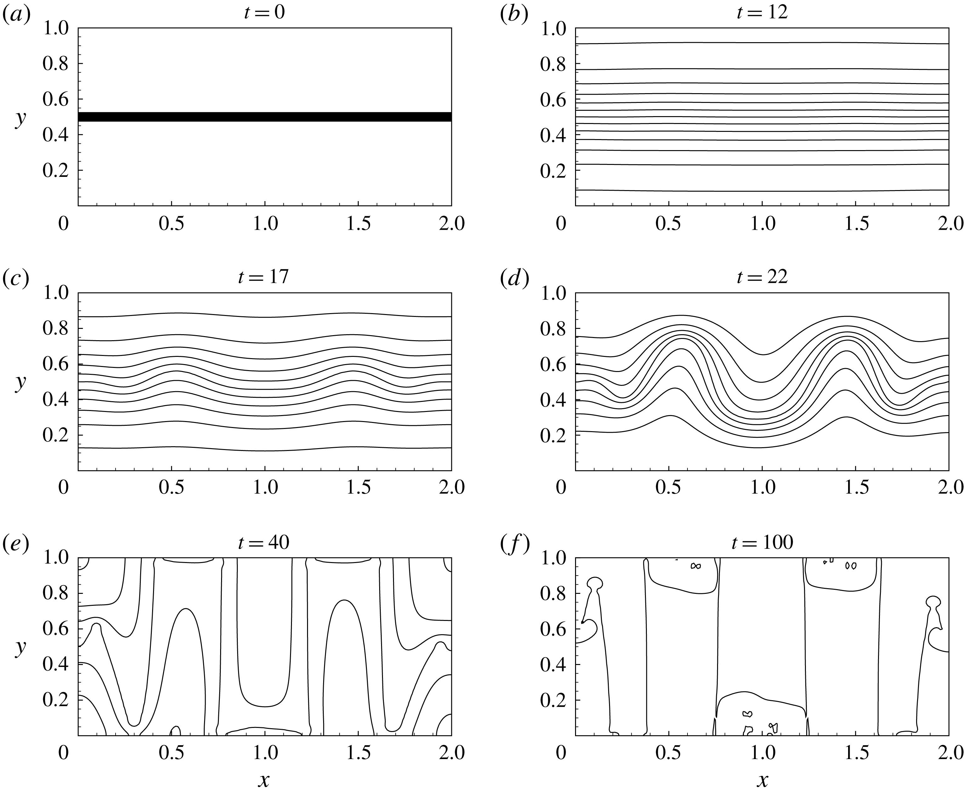
The snapshots of the fields of concentration (isolines) and velocity (vectors). The data are obtained with the use of the phase-field model for $Sc=10^{4}$ and $Gs=10^{5}$ , $M=1$ , $A=-0.5$ and $Cn=2.5\times 10^{-5}$ .

Figure 12.

The snapshots showing the isolines of the of the field of chemical potential. The data are obtained with the use of the phase-field model for $Sc=10^{4}$ and $Gs=10^{5}$ , $M=1$ , $A=-0.5$ and $Cn=2.5\times 10^{-5}$ . The same levels of chemical potential are depicted in all panels.

Figure 13.

(a) The kinetic energy of the average flow, (b) the interfacial energy, (c) the volume of the interface and (d) the average concentration in liquid $1$ versus time. The data are obtained for the runs fulfilled with the use of the phase-field model for $Sc=10^{4}$ , $M=1$ , $A=-0.5$ , $Cn=2.5\times 10^{-5}$ and $Gs=10^{4}$ (dotted line), $Gs=5\times 10^{4}$ (dashed line), $Gs=10^{5}$ (dash-dot-dotted line), $Gs=5\times 10^{5}$ (long-dashed line) and $Gs=5\times 10^{6}$ (solid line).

Figures 11 and 12 illustrate the development of the frozen waves in a heterogeneous binary mixture which evolution is modelled using the phase-field approach. Figure 11 shows the fields of concentration and velocity and figure 12 shows the field of chemical potential. To facilitate the comparisons of the phase-field and classical results the phase-field calculations are performed for the same values of the Schmidt and Gershuni numbers. The phase-field approach, however, also requires the values of three additional parameters: the Mach number, that controls the magnitude of the Korteweg force, is initially set to an intermediate value of $1$ ; the ‘mixture temperature’ is set so as to allow some diffusion between the phases, $A=-0.5$ ; and the Cahn number is $Cn=2.5\times 10^{-5}$ .

Within the phase-field approach the rate of diffusion is determined by the field of chemical potential. At the initial moment the chemical potential has a sharp transition across the interface (see figure 12 a). During the evolution the magnitude of the gradient of the chemical potential rapidly decreases, reducing the intensity of interfacial diffusion, so the diffusive transport becomes completely non-existent at the last snapshot when the binary system almost reaches its state of thermodynamic equilibrium. For $A=-0.5$ , the equilibrium concentrations in each phase are $\pm 0.388$ (if the capillary and vibrational effects are totally neglected), and in figure 13(d) the average concentration $C_{1}$ is quite close to this value near the end of the numerical run ( $t\sim 100$ ).

The snapshots for the classical and phase-field theories look very similar, which indicates that at $M=1$ the Korteweg force remains too weak to significantly affect the dynamics of the mixture. The visible difference between figures 6 and 11 is the level of interface smearing: in the case of the classical approach the thickness of the interface constantly grows, while in the phase-field simulations the interface thickness remains constant almost during the entire numerical run. Another difference between the phase-field and classical results is that for lower Gershuni numbers, when the interface remains flat ( $Gs=10^{4}$ in figures 7 a and 13 a), the intensity of the average flow keeps growing in the classical case, and the level of energy starts decaying at some moment in the case of the phase-field simulations. The formation of the frozen waves occurs due to development of the average motion in the neighbouring liquids, and when this motion becomes critically strong, the shape of the interface is changed. The latter observation indicates that for $M=1$ the threshold Gershuni number is $Gs_{c}=3\times 10^{4}$ .

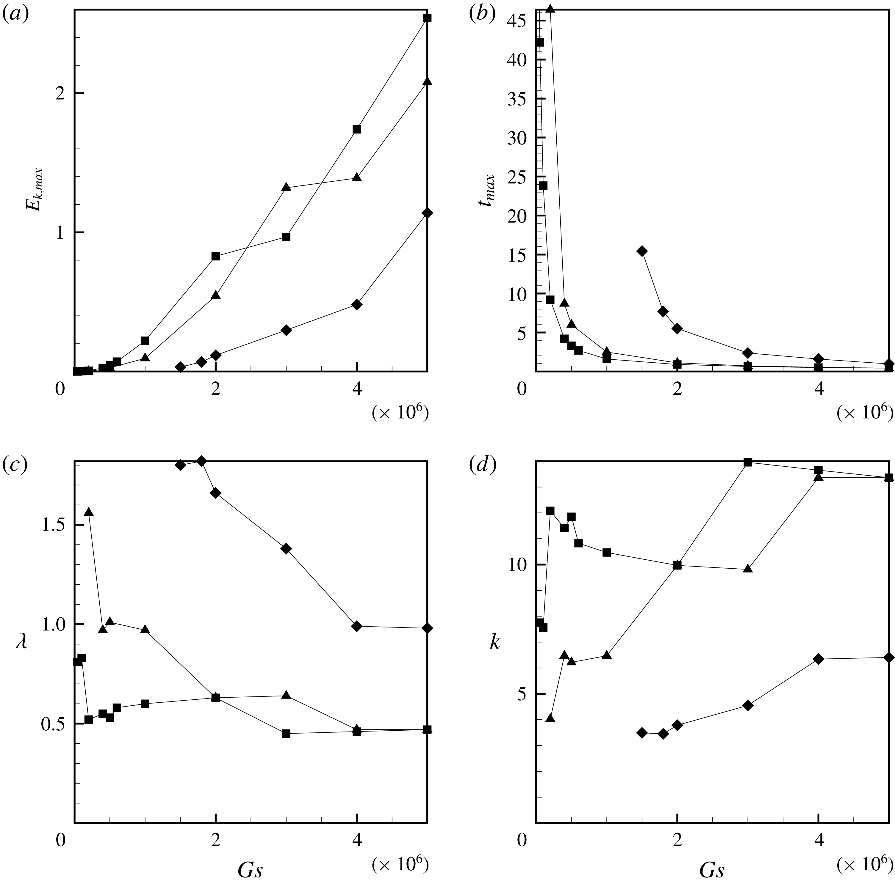
Similarities between the classical and phase-field results are also underlined in figures 9 and 10, where the phase-field data set is distinguished by square symbols. All general features of the dynamics of the binary mixture are very similar to the classical results: the maximum values of the kinetic energy, the time moments when the kinetic energy has a peak and the periodicity of the formed waves almost coincide. Some differences however appear at the higher Gershuni numbers: the development of the instability is characterised by more intensive flows, and the formation of additional waves in a container occurs at slightly higher Gershuni numbers as compared with the classical simulations, which is to be explained by the action of the surface tension forces. Namely, three pillars are formed at $Gs>5\times 10^{4}$ , five at $Gs>2\times 10^{5}$ , seven at $Gs>3\times 10^{6}$ , nine at $Gs>6\times 10^{6}$ and eleven at $Gs>10^{7}$ . The clear differences are also seen at very low Gershuni numbers, closer to the instability threshold. Here, the dynamics of a mixture that is described by a classical model is characterised by stronger interface smearing, which reduces the magnitude of the vibrational force and slows down the development of the frozen wave instability, as compared to the mixture that is described using the phase-field approach.

Figure 14.

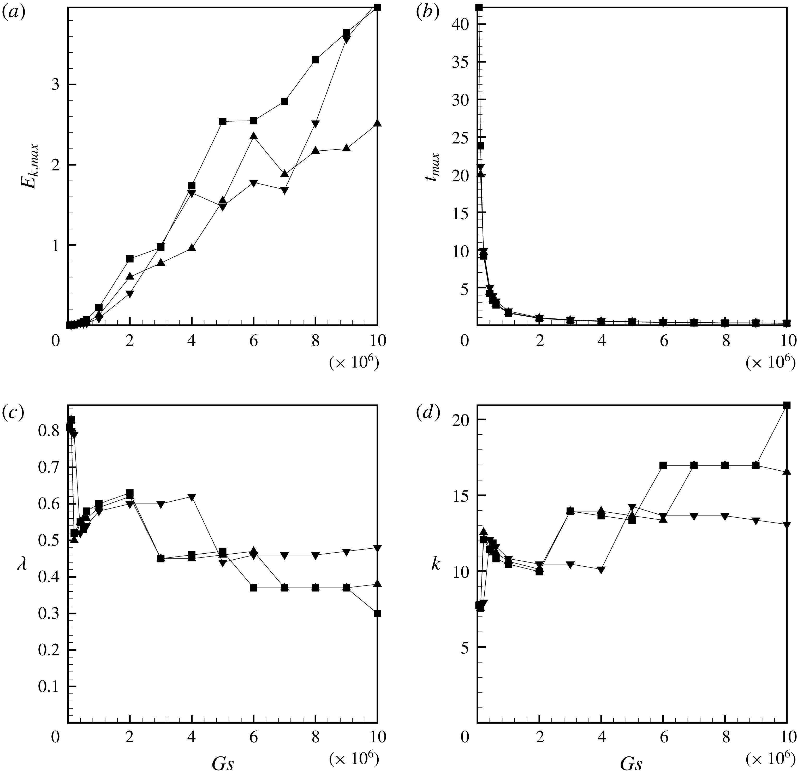
(a,b) The maximum value of the kinetic energy of the average flow and the time moment when the kinetic energy is maximum versus the Gershuni number. (c,d) The wavelengths and the wavenumbers that characterise the periodicity of the frozen waves versus the Gershuni number. The data are obtained for the phase-field model, for the parameters $Sc=10^{4}$ , $Cn=2.5\times 10^{-5}$ , $A=-0.5$ and $M=1$ (‘squares’), $M=0.001$ (‘triangles’) and $M=0.0001$ (‘diamonds’).

Figure 15.

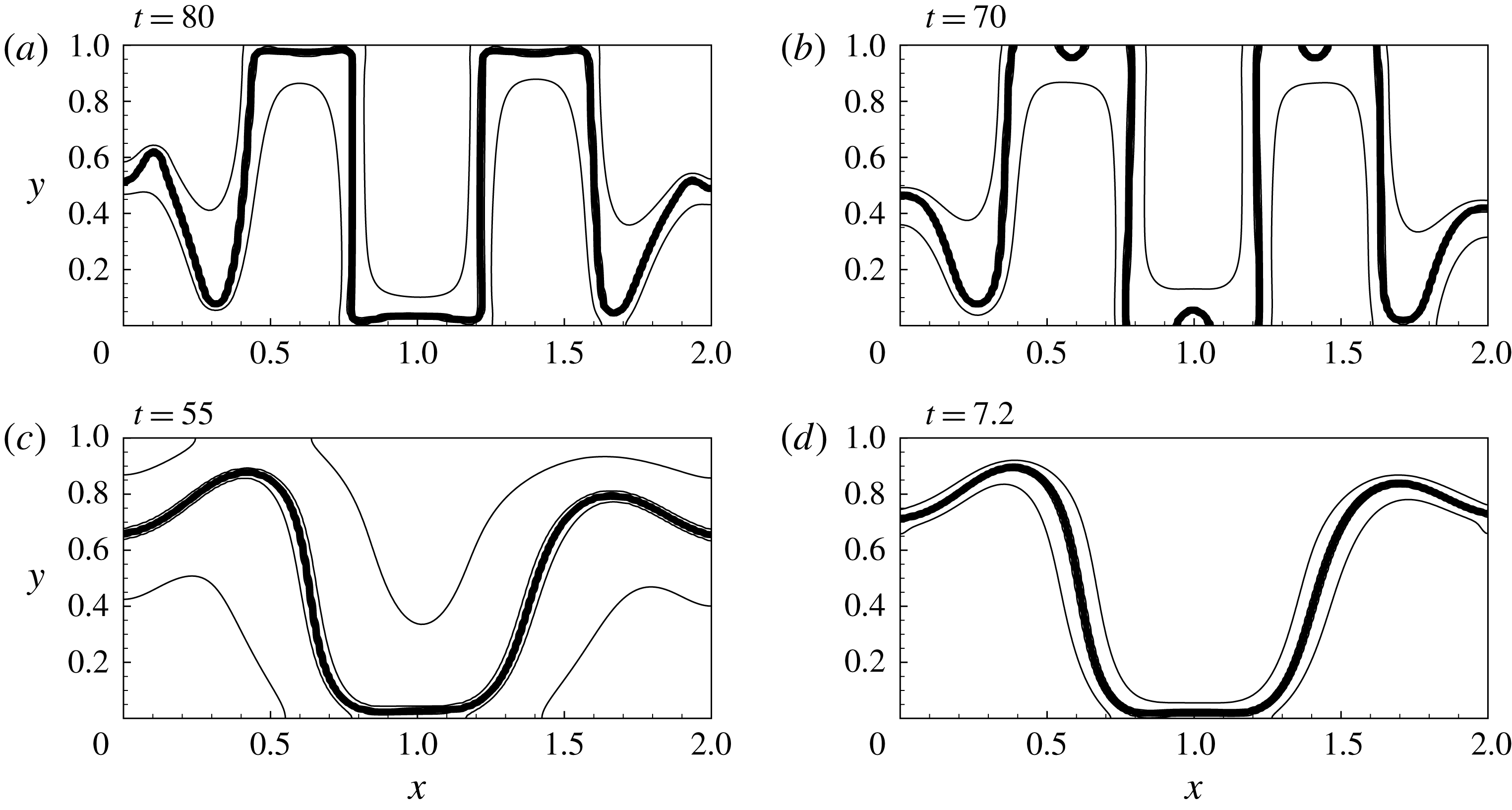
The shape of an interface subjected to the vibrations, for the parameters (a) $M=1$ , $Gs=5\times 10^{4}$ , (b) $M=0.01$ , $Gs=10^{5}$ , (c) $M=0.001$ , $Gs=2\times 10^{5}$ and $M=0.0001$ , $Gs=2\times 10^{6}$ (d). The other parameters are $Sc=10^{4}$ , $A=-0.5$ and $Cn=2.5\times 10^{-5}$ .

Figure 16.

(a) The volume of the interface, (b) the length of the interfacial line, (c) the surface tension coefficient and (d) the average concentration in liquid $1$ versus time. The data are obtained for the runs fulfilled with the use of the phase-field model for $Sc=10^{4}$ , $A=-0.5$ , $Cn=2.5\times 10^{-5}$ , $Gs=5\times 10^{6}$ and $M=1$ (solid line), $M=0.001$ (dashed line), $M=0.0001$ (dotted line).

The above results show that the initially chosen value of the Mach number, $M=1$ , is too low to generate substantial differences between the classical and phase-field simulations. To reveal stronger differences we perform the set of numerical simulations for smaller Mach numbers, $M<1$ . We however found that the influence of the Korteweg force remains insignificant (and the behaviour of the mixture remains very close to the one predicted by the classical equations) for all $M>0.01$ . The clear differences appear when the Mach number is $M=0.001$ and lower. The general dynamics of a mixture always remains similar to the one obtained with the help of the classical approach, however, the threshold Gershuni number required for the ignition of the frozen waves and the levels of vibrations that control the number of the pillars in the container change, which can be seen in figure 14 and in table 1.

Table 1.

The threshold Gershuni numbers, $Gs_{c}$ , the wavenumbers that characterise the periodicity of the critical frozen waves (that are formed under the critical value of the Gershuni number), $k_{c}$ , and the threshold Gershuni numbers predicted by the linear theory versus the Mach number. The other parameters for the numerical runs are $Sc=10^{4}$ , $A=-0.5$ and $Cn=2.5\times 10^{-5}$ . For the classical approach, $Gs_{c}$ determines the level of vibrations when the interface shape becomes primarily determined by diffusion rather than by vibrations.

Figure 15 shows the frozen structures that are formed in a container under the critical vibrational forcing for different Mach numbers. All structures look similar, although the lower the value of the Mach number is, the more elastic the interface becomes, thus reducing the growth of disturbances with shorter wavelengths. In figure 15(c,d) there is only one pillar in the container, with a size of nearly $1$ , half of the container’s length. Such a frozen pattern is the structure with the smallest wavenumber that may be realised in the container. Similar structures were also observed in the experiment (Gaponenko et al. Reference Gaponenko, Torregrosa, Yasnou, Mialdun and Shevtsova2015b ).

We also want to make some further correlations with the linear theory by Lyubimov & Cherepanov (Reference Lyubimov and Cherepanov1986). The non-dimensional form of (1.1) looks as follows:

(3.1) $$\begin{eqnarray}\frac{Gs_{c}M}{2Sc}=\unicode[STIX]{x1D70E}k.\end{eqnarray}$$

Here, we assumed the weightlessness conditions; $\unicode[STIX]{x1D70E}$ is the non-dimensional coefficient of surface tension that is introduced as $\unicode[STIX]{x1D70E}_{\ast }/(\unicode[STIX]{x1D70C}_{\ast }\unicode[STIX]{x1D707}_{\ast }L_{\ast })$ , and that is determined by the integral

(3.2) $$\begin{eqnarray}\unicode[STIX]{x1D70E}=M\frac{E_{i}}{L}=Cn\int _{V}(\unicode[STIX]{x1D735}C)^{2}\,\text{d}V,\end{eqnarray}$$

where $L$ is the length of the interface (for the 2-D problem, $L$ plays the role of the surface area of the interface, and $V$ is the surface area of the computational domain). For calculation of the interface length we may use the volume of the interface and the fact that the interface thickness remains almost constant in the phase-field simulations.

For instance, figure 16 depicts the development of the instability for the different values of the Mach number. Figure 16(a,b) shows the volume of the interface and the length of the interfacial line, and figure 16(c) shows the time changes of the surface tension coefficient, $\unicode[STIX]{x1D70E}$ . If we neglect the initial spikes in the values of this coefficient and focus on the moments when the frozen waves are already fully set, we may say that all three curves converge to approximately one value, $\unicode[STIX]{x1D70E}\sim 0.0006$ , that is primarily determined by the Cahn number. The value of the surface tension coefficient allows us to estimate the critical Gershuni numbers as predicted by (3.1). These numbers are listed in the last row of table 1. All these numbers are different from the actual critical Gershuni numbers, which should be explained by the fact that (3.1) is obtained for an infinite interface while we examine the dynamics of a mixture enclosed in a container, which restricts the range of the wavenumbers. For the classical theory the instability under lower Gershuni numbers is induced by long wave perturbations, with $\unicode[STIX]{x1D706}\rightarrow \infty$ and $k\rightarrow 0$ (see e.g. Lyubimova et al. Reference Lyubimova, Ivantsov, Garrabos, Lecoutre, Gandikota and Beysens2017) that cannot be realised within a confined geometry. Although one sees that when the role of the surface tension forces grows so the wavelength of the critical structure becomes larger, the critical Gershuni numbers predicted by the linear theory (3.1) become closer to the numbers obtained from the numerical simulations.

Figure 17.

(a) The length of the interfacial line, and (b) the surface tension coefficient versus time. The results are shown for $A=-0.5$ , $Sc=10^{4}$ , $Gs=5\times 10^{6}$ , $M=1$ and $Cn=2.5\times 10^{-5}$ (solid lines), $Cn=10^{-4}$ (dashed lines) and $Cn=4\times 10^{-4}$ (dash-dotted lines).

Figure 18.

(a,b) The maximum value of the kinetic energy of the average flow and the time moment when the kinetic energy is maximum versus the Gershuni number. (c,d) The wavelengths and the wavenumbers that characterise the periodicity of the frozen waves versus the Gershuni number. The data are obtained for the phase-field model, for the parameters $Sc=10^{4}$ , $M=1$ , $A=-0.5$ and $Cn=2.5\times 10^{-5}$ (‘squares’), $Cn=10^{-4}$ (‘triangles’) and $Cn=4\times 10^{-4}$ (‘nablas’).

We also performed the numerical simulations for the different Cahn numbers (the results are depicted in figures 5, 17 and 18). The change of this parameter does not introduce any qualitative differences to the dynamics of a binary mixture. The change of the Cahn number alters the surface tension coefficient, which is shown in figure 17, and these changes explain the slight differences in the wave patterns that are formed, as may be observed in figure 18.