Implications
This study is concerned with methods to assist in selecting the best dairy animals in developing dairy sectors such as Pakistan. Limited data are available in these sectors and so selection can be difficult. Genetic evaluation models can be used to help this process but models that are too simple or complex can lead to inaccurate or biased results. Based on the study outcomes, it is recommended to use a repeatability animal model for evaluating the first three lactations in which genetic parameters are estimated as part of the model fitting process.
Introduction
The genetic evaluation model (GEM) used in a country is dependent on the type of dairy system, the population of animals and the number of animals recorded for both performance and pedigree. Throughout the world there are varying levels of development in dairy sectors, and many of them have their own GEM. In developed dairy sectors such as Australia and The Netherlands where the national herd size is ~1.5 million animals, about 45% of animals are being herd-recorded (CRV, 2008; Australian Dairy Herd Improvement Scheme (ADHIS), 2011). In contrast, in developing dairy sectors performance records are seldom kept and therefore there is a vast difference in the options available for the genetic evaluation of animals. For example, in Pakistan there are ~25 million dairy cattle, but the most established progeny testing system in the country records <1000 milking animals per year. Furthermore, in developing dairy sectors, problems can be exacerbated due to the large environmental effects, poor management due to limited resources and poor data quality (Dahlin, Reference Dahlin1998; Ilatsia et al., Reference Ilatsia, Muasya, Muhuyi and Kahi2007). These problems have their implications and potentially reduce genetic gain. For example in developed dairy sectors, evidence shows genetic gains in milk production of ~2% per year (Hill, Reference Hill2010), whereas looking at similar information from Pakistan we can see little to no increase (Khan et al., Reference Khan, Rehman, Khan and Sohail2008). This difference in success is not confined to the Pakistani dairy system, but is common in low-input smallholder systems throughout the world (Rege et al., Reference Rege, Marshall, Notenbaert, Ojango and Okeyo2011).
The primary aim of any GEM is to select animals based on performance-recorded data as accurately as possible to maximize genetic gain in the population. In developed dairy sectors, complex GEMs such as random-regression test-day models are used to account for as much variation as possible within the data (Interbull, 2009). Although a theoretically superior model, it requires sufficient recorded data to ensure the evaluation is accurate. In developing dairy sectors the number of recorded animals can often be very low and hence complex GEMs may not be feasible within their system. This can also occur in developed dairy sectors where there are animals being evaluated from small herds or where traits are recorded only on research farms. In these cases, simpler models involving less computation and requirements for recorded information may be helpful.
A particular problem with a low number of animals in an evaluation is to account for environmental or management effects for animals recorded from the same herd, year and season. These are generally fitted as fixed effects within the evaluation model and account for ~40% of the variation seen in milk and fat yield (Chauhan, Reference Chauhan1987; Van Bebber et al., Reference Van Bebber, Reinsch, Junge and Kalm1997). It is well established that ignoring fixed effects can lead to biased predictions of breeding values (Henderson, Reference Henderson1975a). However, it is also important to consider that when fixed effects are of little consequence, the resultant decrease in the contemporary group (CG) size may lead to an increase in prediction error variance. Furthermore, if records are obtained from closely related animals, then these records contribute little information to the evaluation (Van Vleck, Reference Van Vleck1987; Visscher and Goddard, Reference Visscher and Goddard1993).
Therefore, the aim of this study was to assess the best GEMs to predict breeding values in dairy cattle in Pakistan where there are limited data available. To address this aim, simulated data sets with known breeding values were used and compared with the estimated breeding values (EBVs) from various GEMs. Second, actual herd recorded data from an Australian progeny testing system was divided into subsets resembling the Pakistani progeny testing system. These subsets were then analysed using GEMs and breeding values were estimated and compared using cross-validation (CV).
Material and methods
Overall this study compares a number of different types of GEMs. The main factors considered are: (1) a multivariate (MV) v. a repeatability (RP) model in accounting for production in the first three parities; (2) an animal (ANIM) v. a sire (SIRE) model in modelling the random genetic effects; (3) different fixed effects models to account for effects such as herd, year and season; and (4) fitting a model with genetic parameters fixed v. estimating the genetic parameters as part of the model fitting process.
This was carried out by using historical data from Pakistan’s Sahiwal progeny testing system to provide a basis of the herd structures and sizes. Subsequently, two methods were used for the comparison of models. The first method used simulated data based on the Pakistani progeny testing system. The second method used subsets of actual herd recorded data from the Australian dairy system to provide an indication of how the models compare based on actual industry data. Model comparisons were not carried out on the original Pakistani data set as it was only a single data set with small numbers of records per year and a small number of herds making CV less reliable.
Data
Pakistan milk yield data
Historical data from the Research Centre for the Conservation of Sahiwal Cattle, Jhang, Pakistan (RCCSC, http://www.rccsc.com.pk/), were used in this study as the basis for simulation and analysis. These records included both lactation and pedigree records from five major government Sahiwal herds involved in herd recording since 1968. The herd size of these farms was between 100 and 350 milking animals. In total there were 29 790 lactations from 310 sires and 6895 dams with an average number of lactations per dam of 4.3. The information available for each lactation record was the herd, date of calving, age at calving and in the majority of cases, the sire and the dam of the lactating animal.
Simulated data
Data were simulated based on genetic parameters estimated from a preliminary analysis of the RCCSC herd recorded data (see Supplementary material S1). Specifically, additive genetic effects (breeding values, a) were generated for each of n animals and for three parities from a MV normal N(0,G) distribution where
 $${\bf G}=\left( {\matrix{ {\sigma _{{a_{1} }}^{2} } & {\sigma _{{a_{{12}} }} } & {\sigma _{{a_{{13}} }} } \cr {\sigma _{{a_{{21}} }} } & {\sigma _{{a_{2} }}^{2} } & {\sigma _{{a_{{23}} }} } \cr {\sigma _{{a_{{31}} }} } & {\sigma _{{a_{{32}} }} } & {\sigma _{{a_{3} }}^{2} } \cr } } \right)\,\otimes\,{\bf A}$$
where A is the numerator relationship matrix based on the RCCSC pedigree, and where the additive genetic variances and covariances (σ aij ) were based on the output of the preliminary analysis of the first three parities. Residual effects (e) were generated from a MV normal N(0,R) distribution, where
 $${\bf R}=\left( {\matrix{ {\sigma _{{e_{1} }}^{2} } & {\sigma _{{e_{{12}} }} } & {\sigma _{{e_{{13}} }} } \cr {\sigma _{{e_{{21}} }} } & {\sigma _{{e_{2} }}^{2} } & {\sigma _{{e_{{23}} }} } \cr {\sigma _{{e_{{31}} }} } & {\sigma _{{e_{{32}} }} } & {\sigma _{{e_{3} }}^{2} } \cr } } \right)\,\otimes\,{\bf I}_{n} $$
where the residual variance-covariance matrix (σ eij ) was also based on the preliminary analysis, MV normal data were generated with the rmvnorm (Genz et al., Reference Genz, Bretz, Miwa, Mi, Leisch, Scheipl, Bornkamp and Hothorn2013) function in R Version 3.0.2 (R Core Team, 2013). These additive and residual effects were summed to obtain phenotypes for the first three parities of each animal (y=a+e). Note that no fixed effects were added to the simulated data (though fixed effect terms were included in the model fitting to assess the impact of CG size on the analysis, see below). Subsequently, a sample of second and third parity lactations were removed to mimic the culling and mortality levels seen in the original RCCSC data set. This resulted in 1138, 921 and 698 first, second and third parities, respectively, the same as the original RCCSC data set. This process was repeated 500 times to yield multiple simulated data sets to compare the GEMs in the study.
Actual herd recorded data
For assessing the GEMs on actual herd recorded data it would be difficult to obtain sufficient data sets from Pakistan to compare numerous models. So instead, historical test-day records were obtained from the ADHIS (http://www.adhis.com.au) and were used as a pool of data to draw subsets which resemble the general herd structure of the progeny testing records from Pakistan. In total 178 dairy herds from Victoria with between 100 and 350 milking Holstein–Friesian animals each year from 1993 to 2002 were used to select five herds at random to represent the size of the Pakistani data set. This was repeated 500 times and for each subset of data the test-day records were used to determine an adjusted 305-day lactation yield for the first three parities using the test-interval method (ICAR, 2009).
It is evident that Australian Holstein–Friesian animals do not truly represent the situation of the recorded Sahiwal population in Pakistan. However, for the purposes of this study by repeating the process of randomly selecting five herds of similar herd sizes to the Pakistani situation 500 times, we can assess the effect of different models with respect to fixed and random effects using CV. So although not truly representing the Pakistani situation, conclusions could be drawn from the Australian data by limiting the data included in its analysis.
GEMs tested
Two types of GEM were tested; the RP model (1) and MV model (2). The RP model is
 $${\bf y}={\bf Xb{\plus}Z_{1} a{\plus}Z_{2} p_{e} {\plus}e}$$
where y is the vector of random variables of the recorded trait; b the vector of fixed effects with an incidence matrix X relating observations to effects; a the vector of additive genetic effects (or animal or sire effects) with an incidence matrix Z1
relating observations to random (polygenic animal or sire) effects where the
 ${\bf a} \sim N({\bf 0},\sigma _{a}^{2} {\bf A})$
where A is the numerator relationship matrix and
 $\sigma _{a}^{2} $
is the additive genetic or sire variance; p
e
the vector of random permanent environmental effects with an incidence matrix Z
2
relating observations to permanent environmental random effects where
 ${\bf p_{e}} \sim N({\bf 0},\sigma _{{p_{e} }}^{2} {\bf I})$
where I is the identity matrix and
 $\sigma _{{p_{e} }}^{2} $
is the permanent environmental variance; and e the vector of independent residual effects where
 ${\bf e}\sim N({\bf 0},\sigma _{e}^{2} {\bf I})$
.
The MV model is:
 $${\bf y_{i}} ={\bf X_{i} b_{i} {\plus}Z_{i} a_{i} {\plus}e_{i}} $$
where the terms in the model (2) represent the same as in (1). However, there are now three traits indexed by i (that is parity one, two and three) and instead of a permanent environmental effect (p e ) for each animal there is a genetic (G) and residual (R) variance-covariance matrix such that:
 $${\bf G}=\left( {\matrix{ {\sigma _{{a_{1} }}^{2} } & {\sigma _{{a_{{12}} }} } & {\sigma _{{a_{{13}} }} } \cr {\sigma _{{a_{{21}} }} } & {\sigma _{{a_{2} }}^{2} } & {\sigma _{{a_{{23}} }} } \cr {\sigma _{{a_{{31}} }} } & {\sigma _{{a_{{32}} }} } & {\sigma _{{a_{3} }}^{2} } \cr } } \right)\,\otimes\,{\bf A}\quad {\rm and}\quad {\bf R}=\left( {\matrix{ {\sigma _{{e_{1} }}^{2} } & {\sigma _{{e_{{12}} }} } & {\sigma _{{e_{{13}} }} } \cr {\sigma _{{e_{{21}} }} } & {\sigma _{{e_{2} }}^{2} } & {\sigma _{{e_{{23}} }} } \cr {\sigma _{{e_{{31}} }} } & {\sigma _{{e_{{32}} }} } & {\sigma _{{e_{3} }}^{2} } \cr } } \right)\,\otimes\,{\bf I}$$
assuming the data vector is stored in the form
 $${\bf y}=({\bf y}_{1} ',{\bf y}_{2} ',{\bf y}_{3} ')'$$
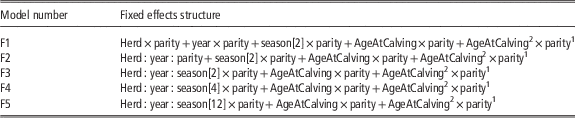
. For both the RP (1) and MV (2) model the random effects structure (Za) and the fixed effects (Xb) can be altered. In this study, the random effects were altered to compare the ‘ANIM’ model with the ‘SIRE’ model and the fixed effects structures (Table 1) were compared to see the impact of CG size and structure on animal evaluation. The number of levels of each fixed effect was herd (five), year (up to 10) and parity (three). The number of levels of season was two, four or 12 as depicted within the brackets of Table 1. Age at calving was fitted as a second order polynomial effect.
Specification of fixed effect model structures
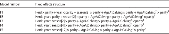
The symbol ‘×’ indicates fields fitted with an interaction and ‘:’ indicates concatenated fields which were fitted without the main effects.
1 The number of levels of season was two, four or 12 as depicted within the brackets.
In each of the simulated and actual herd recorded data runs, there were 20 models fitted and compared. That is, two model types (RP and MV), with two random effect structures (ANIM and SIRE) and five fixed effects structures (F1 to F5, from Table 1). All models were fitted using ASReml-R Discovery Edition 1.0 (Butler et al., Reference Butler, Cullis, Gilmour and Gogel2009).
The models were fitted with the estimation of genetic parameters included in the model fitting process, as well as fitted using fixed genetic parameter values. These fixed parameter values were obtained from the different analyses of: (1) the original RCCSC data that were used for the simulation study and (2) the entire Australian dataset of 178 herds. Details of these values can be found in Supplementary material S1 and S2.
Comparison of models
Convergence and estimation of genetic parameters
When genetic parameters are fixed, the model fitting process requires one non-iterative BLUP run to solve the generalized least squares equations and therefore every model successfully returns estimates of fixed and random effects (e.g. breeding values). If genetic parameters are estimated as part of the model fitting process, the REML iteration process may fail to converge. Where parameters were estimated, the percentage of model fittings that converged was used to assess the robustness of each model. In addition, the heritability (h 2), genetic correlation (r g ) and other genetic parameter estimates of these models were compared to the ‘true’ simulated values (Supplementary material S1) and ‘gold standard’ values obtained from the analysis of the ADHIS data set of 178 herds (Supplementary material S2).
Mean square error of prediction
For determining the ‘best’ model in each study, a mean square error of prediction (MSEP) was calculated and used to compare the ability of the model to estimate breeding values. In the simulation study, the simulated breeding values were compared directly with the EBVs predicted by each of the models. For the MV models, the EBVs were averaged over the three parities to yield a single EBV for comparison with the RP models. The MSEP was calculated for each model according to equation (3) (Mevik and Cederkvist, Reference Mevik and Cederkvist2004).
 $$MSEP_{1} =\mathop{\sum}\limits_{i=1}^n {({\rm SimulatedBV \,{- } \,EstimatedBV})^{2} } /n$$
where n is the number of records in the subset of data.
In the study using subsets of actual herd recorded data from Australia, the true breeding values were unknown. Therefore, adjusted milk yields were calculated by subtracting the fitted fixed effects from the raw milk yields using the most complex model (MV-ANIM-F5) to the whole Australian dataset of 178 herds. These adjusted yields (
 $$y^{{\asterisk}} =\hat{a}{\plus}\hat{e}$$
for the MV and
 $$y^{{\asterisk}} =\hat{a}{\plus}\hat{p}_{e} {\plus}\hat{e}$$
for the RP) were compared to predicted sire effects (predicted yields;
 $\hat{y}=\hat{s}$
for the SIRE models) or additive genetic effects (predicted yields;
 $\hat{y}=\hat{a}$
for the ANIM models).
A CV procedure was conducted to assess the ability of the models to estimate breeding values with smaller subsets of data. This was repeated ten times for each model in every run. In this procedure, 90% of the animals in the subset of the data for each run were selected at random and used to fit the model. The remaining 10% had their yields predicted using the model output. The MSEP for the analysis using actual herd recorded data was calculated for each of the 10 CV procedures using the following equation (Mevik and Cederkvist, Reference Mevik and Cederkvist2004):
 $$MSEP_{{\rm 2}} =\mathop{\sum}\limits_{i=1}^n {({\rm AdjustedYield \,- \,PredictedYield})^{2} } /n$$
An average of the 10 CVs was taken to be the MSEP 2 for that particular model and run. For both the simulation method and the CV method using actual data, the model yielding the lowest MSEP 2 for each run was considered to be the ‘best’ model for that particular data set.
Sire ranking
The correlation and corresponding rankings of the EBVs of the sires evaluated was used as a secondary check on the differences between models. For each subset of data, the EBV of all sires with greater than five daughters was compared with the ranking according to: (1) the true BVs for the simulation study; and (2) the EBVs from the ‘gold standard’ model output (MV-ANIM-F5) for the study on actual data. This is an important verification step as the sire ranking and selection is the primary outcome following the genetic evaluation process.
Results
Convergence
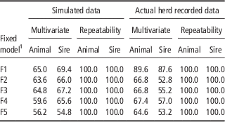
When genetic parameters were estimated, the results for both the simulated data sets and the subsets of actual herd recorded data (Table 2) show the RP model was the most robust model as it had the highest success rate of model fittings. With the MV models, the convergence rates are much lower than the RP models suggesting that these models fail to estimate the genetic covariance between parities one, two and three. Within the simulated data sets, the SIRE model was slightly more successful than the ANIM model in contrast to the results from the actual herd recorded data in which the ANIM model was more successful. Models that failed to converge were not included in subsequent analysis or calculations.
Percentage of converged models for the 500 simulated data sets and 500 subsets of actual herd recorded data where genetic parameters were estimated as part of the model fitting process
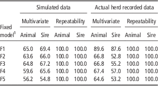
1 Fixed model: F1 to F5 refer to the fixed effects structures described in Table 1.
Simulated data
Estimation of genetic parameters
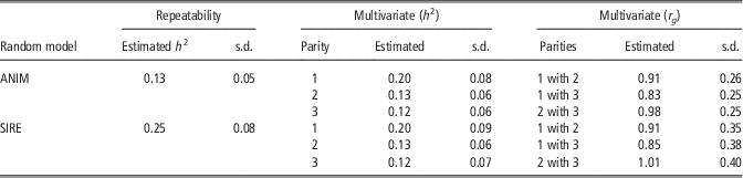
When genetic parameters were estimated on the simulated data sets, the average results (Table 3) from the RP models show that ANIM models yield a h 2 estimate (0.13) that is close to the average ‘true’ value of parities one, two and three (0.15), but the SIRE models overestimate this value (0.25). With the MV models, both the ANIM and SIRE model estimates of h 2 were also very close to the ‘true’ values (0.201, 0.121 and 0.116). Similarly, the r g estimates for both the MV-ANIM and MV-SIRE models differed little from the ‘true’ values (0.92, 0.85, 0.98). However, the standard deviations on the r g estimates of MV-ANIM (ranging from 0.25 to 0.26) are much lower than those of the MV-SIRE model (0.35 to 0.40) indicating that the MV-ANIM model had greater precision.
Estimated genetic parameter values from the simulated data sets using repeatability and multivariate for both the ANIM and SIRE models averaged across all fixed effects structures
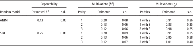
The ‘true’ simulated heritability values for parities one two and three were 0.201, 0.121 and 0.116. The ‘true’ r g values were 0.92 for parities 1 and 2, 0.85 for parities 1 and 3 and 0.98 for parities 2 and 3.
Model comparison
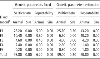
The percentage out of 500 runs where each individual model was considered to be the ‘best’ model according to the lowest MSEP 1 can be seen in Table 4. This was determined separately for models were genetic parameters were fixed and estimated. An overall result from Table 4 is that the SIRE model was seldom the model with the lowest MSEP 1. When genetic parameters were fixed, the results show that the MV-ANIM-F1 model is superior to all the other models. However, if genetic parameters are estimated, the RP-ANIM-F1 model is superior. More generally, comparing within the same fixed effect structure, MV models are superior when genetic parameters are fixed, RP models are superior when the parameters are estimated (Table 4).
Percentage of times from 500 simulated data sets that the specified model had the lowest MSEP 1
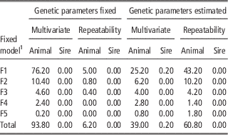
This was calculated separately for models when genetic parameters were fixed and estimated.
1 Fixed model: F1 to F5 refer to the fixed effects structures described in Table 1.
Sire ranking
The correlation between the sire EBVs of the different tested models with the ‘true’ EBVs ranged from 0.969 to 0.983 with standard deviations of ~0.01 for all models. These values demonstrate that sire rankings between the models varied very little.
Actual herd recorded data
Estimation of genetic parameters
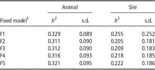
The average estimates of h 2 for both the RP-ANIM and RP-SIRE models can be seen in Table 5. Compared with the average ‘gold standard’ h 2 (0.384) it can be seen that all the RP models underestimate this value. Furthermore, the RP-ANIM estimates are closer to the ‘gold standard’ than that of the RP-SIRE. Considering only the RP models, the RP-ANIM-F1 model was the one with the closest h 2 estimate to the ‘gold standard’.
Average estimates of heritability (h 2) of the actual herd recorded data and their standard deviations for the repeatability models of 500 subsets of data
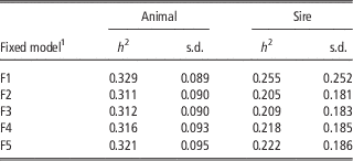
1 Fixed model: F1 to F5 refer to the fixed effects structures described in Table 1.
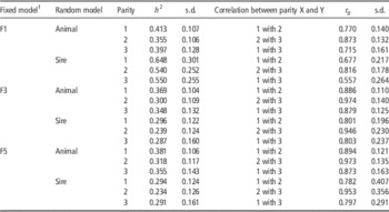
The average estimates of genetic parameters for the MV analyses can be seen in Table 6. The results for the F2 and F4 models are not shown here, but they were similar to those presented for F3. From Table 6 we can see that the h 2 estimates for the F1 are higher than that of F3 and F5. In addition, the estimates for the r g between parities when using the F1 model are lower. Comparing these values to each other, it seems that the h 2 of the MV-ANIM-F1 model are the closest to the ‘gold standard’ (0.429, 0.344 and 0.378). However, the r g values of the F1 model are very low compared with the ‘gold standard’ (0.945, 0.926 and 0.996). Contrastingly, the MV-ANIM-F5 model estimates of r g are much closer to the ‘gold standard’ than that of the MV-ANIM-F1 but the h 2 estimates are slightly lower. Despite this, it seems that the MV-ANIM-F5 model estimates are the closest overall.
Average estimates of genetic parameters (r g , h 2) for parities one, two and three and their standard deviations as calculated from the F1, F3 and F5 multivariate models on actual herd recorded data

1 Fixed model: F1 to F5 refer to the fixed effects structures described in Table 1. The results for the F2 and F4 models are not shown here, but they were similar to those presented for F3.
The greatest difference from these results is between the h 2 and r g estimates from the ANIM and SIRE models. Not only do the estimated values differ, but the standard deviation values from the SIRE model are much higher than the ANIM. This again suggests that the ANIM model is more precise with data sets of this size.
Model comparison
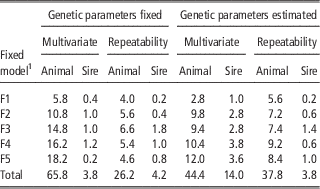
Using MSEP 2, Table 7 shows the percentage of times where each model was considered ‘best’ when genetic parameters were fixed or estimated. When genetic parameters were fixed, the MV model (69.6%) was superior to the RP (30.4%), the ANIM model (92.0%) was superior to the SIRE (8.0%) and the fixed effects models F3 (24.2%), F4 (23.8%) and F5 (23.8%) were considered superior more often than the F1 (10.4%) and the F2 (17.8%) models. When genetic parameters were estimated, the MV (44.4%) and RP (37.8%) models were similar, the ANIM model (82.2%) was still superior to the SIRE (17.8%) and models with increasing complexity of fixed effects were more frequently the best model (F1 to F5: 9.6%, 18.4%, 21.0%, 24.0% and 25.0%).
Percentage from 500 runs that the specified model had the lowest MSEP 2 for the subset of five selected herds from the actual herd recorded data
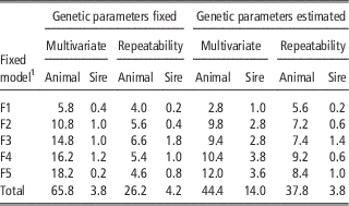
1 Fixed model: F1 to F5 refer to the fixed effects structures described in Table 1.
The overall outcome using actual herd recorded data shows that when genetic parameters are fixed or estimated, the MV-ANIM-F5 model is considered to be the superior model. This is in contrast to the results from the simulated data study which determined the MV-ANIM-F1 model to be superior when parameters were fixed and the RP-ANIM-F1 when parameters were estimated.
Sire ranking
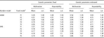
Despite the differences in the MSEP 2 the correspondence between the sire rankings from the output of each of the models varied very little for the herd recorded Australian data (see Table 8). These results show that the number of sires ranked in the top 10 sires from each model output had a narrow range with the lowest average across all models being 3.37 (MV-SIRE-F1) and the highest average value at 4.31 (MV-ANIM-F2 and RP-ANIM-F2). Furthermore, the correlation between the EBVs of the different tested models with the ‘gold standard’ EBVs ranged from 0.980 to 0.985 with standard deviations of ~0.01 for all models. These statistics demonstrate that sire rankings between the models compared were both highly correlated and showed little variation in selection outcomes.
Mean number of corresponding sires with the ‘gold standard’ model in the top 10 breeding value rankings when calculated from actual Australian herd recorded data using both fixed and estimated genetic parameters

1 Fixed model: F1 to F5 refer to the fixed effects structures described in Table 1.
Discussion
Data
The primary aim of this research was to assess the best GEMs to predict breeding values in Pakistani dairy cattle when there are limited data available.
Before discussing the results, it is important to first highlight some key assumptions that will affect breeding value estimation in any situation where data may be limited or of poor quality. A key problem is the accuracy of the pedigree information. Research shows that pedigree misidentification is common (Visscher et al., Reference Visscher, Woolliams, Smith and Williams2002; Weller et al., Reference Weller, Feldmesser, Golik, Tager-Cohen, Domochovsky, Alus, Ezra and Ron2004, Sanders et al., Reference Sanders, Bennewitz and Kalm2006) and can reduce the accuracy of breeding values and hence reduce genetic gain (Sanders et al., Reference Sanders, Bennewitz and Kalm2006). This is likely to be an even greater problem in Pakistan, but in the short-term is unavoidable. Therefore, for the purposes of this study it is assumed that the pedigree errors will have an equal effect on the different models tested. Keeping this in mind, the outcomes of this work are discussed below relating to convergence rates, estimation of genetic parameters, and finally the choice of model.
Convergence
From both the simulated data and actual data it was apparent that when using small data sets, a high number of MV model fittings failed to converge when genetic parameters were estimated. This suggests that these models may not be suitable and instead a RP model would be more appropriate, because fewer parameters need to be estimated. Comparing between the ANIM and SIRE models the rates differed slightly between the two data sets. However, this difference is more likely a reflection on the depth of pedigree rather than an implication for the model of choice. The pedigree for the Australian data is more accurate and contains fewer gaps in parental information than the Pakistani pedigree used for the simulation. For this reason, the advantages of the ANIM model over the SIRE model could not be exploited with the simulated data, whereas in contrast, the Australian data could.
Estimation of genetic parameters
Results from both the simulated data and actual herd recorded data show that in some cases although model fittings may converge and yield genetic parameter estimates, they may yield biased genetic parameters or violate assumptions made. For example, the MV model r g estimates, although close, are less than one and the variance components of the first three parities are quite different (Supplementary material S2). These values suggest that the RP model assumption, that each parity is genetically the same trait, is not correct. This is consistent with the literature which generally reports the three parities as separate traits (Weller, Reference Weller1986; Schaeffer et al., Reference Schaeffer, Jamrozik, Kistemaker and van Doormaal2000; Powell and Norman, Reference Powell and Norman2006). Furthermore, the ANIM model would be more suitable than the SIRE model as the genetic parameter estimates are closer to the correct values and much more precise as shown by the lower standard deviations.
Looking further into the MV results from the actual herd recorded data (Table 6), estimates of h 2 in the F2 to F5 SIRE models were generally lower, by 20% to 30%, compared with both the ANIM models and the ‘gold standard’ using the whole Australian dataset (Supplementary material S2). This is presumably due to the inclusion of more complete relationships in the ANIM model as ignoring relationships that exist results in a reduction of estimates of genetic variance (Henderson, Reference Henderson1975b). In contrast to the h 2 estimates, the estimates of r g were not so much affected by the random effects in the model (ANIM or SIRE) as expected (Dong et al., Reference Dong, Van Vleck and Wiggans1988). However, the r g estimates from the ANIM model were still closer to the ‘gold standard’ and more accurate than the SIRE model. The results from the simulated data concur with these general outcomes from the actual herd recorded data and therefore they indicate that the ANIM model is superior to the SIRE model when it comes to estimating genetic parameters.
Lastly, looking at the different fixed effects structures, the results from the actual herd recorded data (Table 6) show that the r g values of the F1 model are very low compared with the ‘gold standard’ whereas the more complex fixed effects models (F2 to F5) yield estimates that are much closer to the gold standard. This is an expected but important result, which is consistent with the idea that ignoring fixed effects can lead to biased estimates of variances and correlations (Henderson, Reference Henderson1975c; Van Bebber et al., Reference Van Bebber, Reinsch, Junge and Kalm1997).
Another option considered in preliminary comparisons of this study was to treat some CGs as random effects. Although showing promising results, a number of studies explain that this is only suitable if sires are randomly spread across CGs (Chauhan, Reference Chauhan1987; Meyer, Reference Meyer1987; Visscher and Goddard, Reference Visscher and Goddard1993). This is generally not the case with the Pakistani data set used in this study and hence it was removed from the final analysis.
Model choice
The conclusions on the ‘best’ model from the simulated data and the actual herd recorded data are slightly different. Results from the simulated data (Table 4) indicate that the best model is a MV-ANIM-F1 model when using fixed genetic parameters, but the best model is a RP-ANIM-F1 model when genetic parameters are estimated. The superiority of the RP model over the MV model when parameters were estimated is partially due the lower success rates when fitting the MV models. In contrast, results from actual herd recorded data for both the fixed and estimated genetic parameters (Table 7) show that a MV-ANIM-F5 model is considered the best. The contrast in the model superiority between the simulated and actual data suggests that when genetic parameters are estimated, the MV models are more accurate with the actual data than with the simulated data. This is likely due to the pedigree of the actual herd recorded data being deeper than that of the simulated data (based on the RCCSC data set).
The results of the most superior fixed effects structure differ between the simulated and actual herd recorded data. This makes it difficult to determine a general recommendation from this study alone. These contrasting results may be due to the method of evaluation. Using the simulated data, EBVs were compared with simulated BVs (based on an MV-ANIM-F1 model). With the real data results, EBVs were compared with phenotypic yields corrected for fixed effects based on outputs from the ‘gold standard’ model (from the MV-ANIM-F5 model). The CV results may therefore be biased towards the ‘gold standard’ model. Nevertheless, both the CV and simulation methods generate knowledge about the behaviour of the different models. This is in addition to the more common method of comparing models using the correlation of EBVs from model outputs (Wiggans and Goddard, Reference Wiggans and Goddard1997; Mostert et al., Reference Mostert, Theron, Kanfer and van Marle-Koster2006). Further research comparing between fixed effects structures could be beneficial if it could link the superiority of models with information based on relationships between CGs.
Overall, the results of this study show that given a limited data set, the top 10 sires do not correspond entirely with the true top 10 ranking sires. In a practical sense, this means the accuracy and hence the genetic gain will be reduced. However, this difference is apparent regardless of the model choice as the sire rankings and correlations are similar from all the models compared. This similarity between the models shows that the accuracy and genetic gain of all the models would differ very little. Despite the little difference in the ranking and thus selection outcomes between models, recommendations can still be made on the suitability and robustness of the categories of GEM, rather than choosing a superior individual model.
First, the results suggest that if accurate genetic parameter values can be obtained from a separate source, then it is better to fix them rather than estimate them as part of the model fitting process. However, a complication arises when determining the value of the fixed genetic parameters and the effect on the evaluation outcomes. In single trait selection, errors in estimates of genetic parameters are overcome by the robustness of BLUP, but in multiple trait selection small errors in estimated (or fixed) values can dramatically reduce the accuracy of selection (Henderson, Reference Henderson1984). For this reason it would be recommended to estimate genetic parameters as part of the model fitting process while ensuring genetic parameter estimates fall within a realistic range before interpreting any EBV outputs.
Second, based on the MSEP criterion in both the simulated and actual data sets, the ANIM model was generally more appropriate than the SIRE model. With these comparisons, it is important to consider that the SIRE model is slightly disadvantaged in the calculation method of MSEP with the actual data. This is because the residual variance contains 75% of genetic variance and hence the SIRE models would always have a larger MSEP. However, with the simulated data the comparisons between EBVs were more definitive and in this case, the ANIM model was clearly the superior model.
An interesting discussion point of this study is the suitability of RP model v. the MV model. Although the literature agrees that the first three parities are separate traits and the results from the data analysed in this study concur with this, the outcomes of this study recommend that the RP model would be more suitable for genetic evaluation in Pakistan. This is for two main reasons. First, from Table 2 it is apparent that with both simulated data and actual data, there is a high proportion of failed MV models suggesting that it may be difficult to fit these models in the Pakistani situation. Second, the results from the actual data (Table 7) suggest that if genetic parameters are to be estimated then there is little difference between the models (MV; 44.4%, RP; 37.8%) whereas from the data simulation, which is based on Pakistani data (Table 4), there is a much greater difference with the RP (60%) model being superior to the MV (40%).
Given the general recommendations discussed here, if we focus the results from this study on only the RP-ANIM models where genetic parameters are estimated a closer examination of the fixed effects models can be carried out. These results show clearly that the F1 model is superior (43.2%) more times than models F2 to F5 (10.2%, 4.2%, 1.4% and 1.8%) when using the simulated Sahiwal data (Table 4). However, when using the actual herd recorded data the distinction is not as clear with the model superiority being very similar ranging only from 5.6% to 9.2% (Table 7). Therefore, as discussed earlier it is difficult to recommend a specific fixed effects structure for data sets of limited size. This aligns with the generally accepted view that every data set and structure is unique and hence it is difficult to make general statements about the most suitable model to analyse it (Henderson, Reference Henderson1975c). Consequently, we would refer to the general recommendation in the literature to keep the average CG size between 8 and 25 and to have no less than three records within each CG (Urgate et al., Reference Urgate, Alenda and Carabano1992; Van Bebber et al., Reference Van Bebber, Reinsch, Junge and Kalm1997).
Conclusions
This paper aimed to select and recommend the best model to use for genetic analysis in Pakistan’s dairy sector where limited data are available. Although a specific fixed effects model structure could not be chosen, broad recommendations can be given regarding the type of GEM to be implemented. The main outcome of this research suggests that applying a RP animal model where genetic parameters are estimated appeared to be the best GEM for the Pakistani Sahiwal progeny testing system.
Acknowledgements
The authors would like to acknowledge the Australian Dairy Herd Improvement Scheme and the Research Centre for the Conservation of Sahiwal Cattle (Jhang, Pakistan) from where the historical test-day records and pedigrees were obtained from.