I. INTRODUCTION
The mechanical properties of a material around high-stress areas such as the tip of a fatigue crack vary with the movement of the solute atoms. For example, it has been reported that the mechanical properties change with strain aging around the tip of a non-propagating crack on the fatigue limit of carbon steel. Reference Sinclar1–Reference Lipsitt and Wang3 Moreover, the mechanical properties around the tip of a fatigue crack in a hydrogen gas environment change with the hydrogen concentration. Reference Birnbaum and Sofronis4,Reference Nishikawa, Oda and Noguchi5 These changes in the mechanical properties are localized, and the authors considered that a nano-indentation technique Reference Doerner and Nix6,Reference Oliver and Pharr7 can be used to measure them. A series of the authors' studies is presently being conducted with the ultimate purpose of determining the mechanical property changes that occur with the movement of the solute atoms. As the first step, a method for determining the local mechanical properties (Young's modulus E, Poisson's ratio ν, yield strength σY and work hardening factor n) by indentation is proposed in this study.
The determination of the local mechanical properties of materials by indentation has been the subject of several previous studies. Reference Oliver and Pharr7–Reference Kang, Becker and Sun13 Oliver and Pharr, Reference Oliver and Pharr7 and Pharr et al. Reference Pharr, Oliver and Brotzen8 used the initial part of the unloading curve of the load–depth relation to determine E. Zorzi and Perottoni Reference Zorzi and Perottoni9 used Vickers hardness in addition to determine ν. By their methods, only E and ν could be determined. Although Bucaille et al., Reference Bucaille, Stauss, Felder and Michler10 and Akatsu et al. Reference Akatsu, Demura, Shinoda and Wakai11 used multiple indenters that had different apex angles to determine the mechanical properties of a material, the determination at a specific point of a material with its accuracy was not undertaken, because the mechanical properties could not be determined without changing the indenter and the measurement point. Bouzakis and Michailidis, Reference Bouzakis and Michailidis12 and Kang et al. Reference Kang, Becker and Sun13 compared the relationship between stress–strain and load–depth relation by using finite element method (FEM) analyses, used the initial part of the loading curve of the load–depth relation, and determined the mechanical properties at a specific point of a material. However, because an initial part of a real loading curve is greatly subject to an influence of the surface condition, the accuracy of the determined mechanical properties obtained by experiments may be insufficient. Furthermore, all of the previous studies were limited to specific cases, and the analytical errors were not examined.
Therefore, in the present study, a method for determining the mechanical properties of a specific point of a material was developed and the accuracy was verified. The method utilizes an indenter that combines the characteristics of spherical and conical indenters and can be used to produce multiple indents at a single point.
II. METHODS FOR DETERMINING LOCAL MECHANICAL PROPERTIES
A. Characteristics of unloading process
The inclination k at the just-unloading point on the P–h diagram of an indentation test is given by the following equation Reference Oliver and Pharr7 :
 $$k = {\left. {{{{\rm{d}}P} \over {{\rm{d}}h}}} \right|_{{P_{\max }}}} = {2 \over {\sqrt \pi }}{E_{\rm{r}}}\sqrt A \quad ,$$
here, E r is the reduced Young's modulus of the specimen material due to the effect of the mechanical properties of the indenter (this will be discussed further later), and A is the projected elastic contact area between the indenter and the specimen. Although Eq. (1) is for a cylindrical punch, Reference Sneddon14 it is also applicable to axial-symmetry indenters such as spherical and conical indenters. Reference Pharr, Oliver and Brotzen8 E r is given by the following:
 $${1 \over {{E_{\rm{r}}}}} = {{1 - {\nu ^2}} \over E} + {{1 - {\nu _{\rm{i}}}^2} \over {{E_{\rm{i}}}}}\quad ,$$
here, E i and νi are the Young's modulus and Poisson's ratio of the indenter, respectively. Although the reduced Young's modulus E r may be applied to the specimen material, such is only valid when the Young's modulus of the material is about 100 GPa. In the case of materials such as ceramics that have high Young's moduli and low Poisson's ratios, the error in the determined Young's modulus would be 50% or more. Reference Zorzi and Perottoni9 The correct determination of the Young's modulus therefore also requires the correct determination of the Poisson's ratio.
In this study, the Young's modulus of the indenter is sufficiently large compared to that of the specimen material. Consequently, the second term on the right-hand side of Eq. (2) can be ignored, and Eq. (1) can be rewritten as follows:
 $$k \cong {2 \over {\sqrt \pi }}{E \over {1 - {\nu ^2}}}\sqrt A \quad .$$
In Eq. (3), A is dependent on the mechanical properties of the specimen material and the indentation displacement h. To determine A, it is necessary to measure the contact area under the loaded condition, which is quite difficult. However, k can be easily measured at the same time as the load and displacement using an indentation instrument.
The method for determining E and ν from the measured k using Eq. (3) is described below. If only E is unknown, by conducting a numerical analysis to obtain the arbitrary indentation displacement h of the specimen, E can be determined based on the assumption that the inclination at the just-unloading point is equal to k. If both E and ν are unknown, numerical analyses can be conducted for two different displacements h 1 and h 2, and the unknown parameters determined by a simultaneous solution of the two equations that, respectively, satisfy the two corresponding measured values of k 1 and k 2. However, because the relationship between E and ν for the two indentation displacements would be similar, the determined values of the parameters are likely to contain large errors. The reason for this will be discussed later using Fig. 5. The use of two indents produced by two different indenters with different apex angles has been proposed for reducing this error. Reference Akatsu, Demura, Shinoda and Wakai11 However, this method also produces significant differences between the two relationships between E and ν, and its error is therefore still significant.
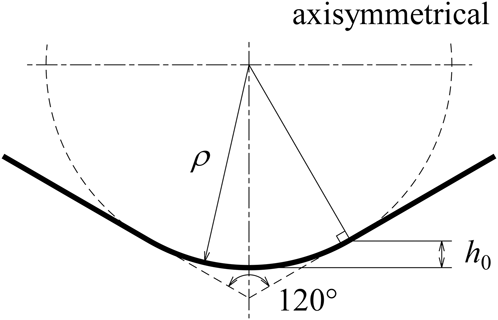
We thus developed a method for determining the mechanical properties of a material at an arbitrary specific point using a conical indenter with a spherical tip of a certain curvature. Figure 1 shows the shape of the indenter tip used in this study. The radius of the curvature of the spherical part that is the indenter tip is ρ, and the apex angle of the conical part is α = 120°. h 0 shows the boundary between the spherical part and the conical part. Since h 0 becomes large when α becomes small, α was decided so that the h 0 could be enlarged. In addition, the friction influence was considered to be avoided, and therefore α was set to 120°. According to Bucaille et al., Reference Bucaille, Stauss, Felder and Michler10 if α is 120° or more, the friction has no significant influence on the normal force in the power hardening material. The critical angle of the friction influence was assumed to be also the same in the linear hardening material used in this study. Then, the validity of the proposed method is the same as that of the case when α is 120° or more, and one can obtain similar results within the range of α. The range of α includes α = 140.6° that is equivalent to the Berkovich and Vickers indenter. The method involves the use of two indentation displacements h 1 (<h 0) and h 2 (>h 0). Only the spherical tip is used for the indentation displacement h 1, and the indent can be considered as a spherical indenter. Reference Field and Swain15 In the case of the displacement h 2, the indent can be considered as a conical indenter. Reference Cheng and Cheng16 A single indenter is thus used to produce two types of indents to obtain k 1 by h 1 and k 2 by h 2.
Shape of the indenter tip used in this study.

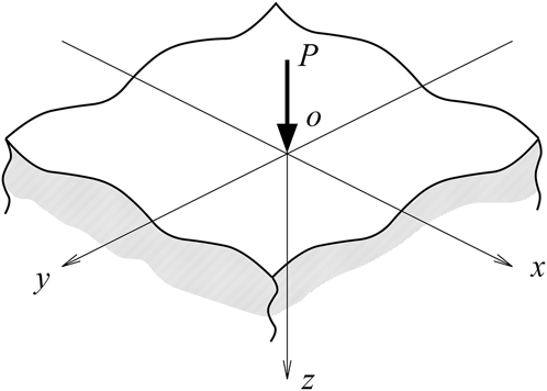
By using Eq. (3), in an axisymmetric solution for either elastic or elastic–plastic material, the Young's modulus E and Poisson's ratio ν can only be determined to the extent of E/(1 − ν2), therefore E and ν cannot be separated any further. Equation (3) contains the basic assumption that during the initial withdrawal of the indenter, the contact area between the indenter and the specimen remains constant, Reference Pharr, Oliver and Brotzen8 and Pharr et al. Reference Pharr, Oliver and Brotzen8 revealed that even when the contact area changes continuously as the indenter is withdrawn, the initial unloading curve of the P–h diagram can be used. On the other hand, the extreme case is to say that point contact is considered. Here, the Boussinesq's equation Reference Johnson17 is referred. The z-direction displacement u z produced by a concentrated point force P acting normally to the elastic half space at the origin (Fig. 2) can be expressed as follows.
 $${u_z} = {P \over {4\,\pi \,G}}\left\{ {{{{z^2}} \over {{{\left( {{x^2} + {y^2} + {z^2}} \right)}^{{3 \mathord{\left/ {\vphantom {3 2}} \right. \kern-\nulldelimiterspace} 2}}}}} + {{2\,\left( {1 - \nu } \right)} \over {{{\left( {{x^2} + {y^2} + {z^2}} \right)}^{{1 \mathord{\left/ {\vphantom {1 2}} \right. \kern-\nulldelimiterspace} 2}}}}}} \right\}\quad ,$$
where G is the shear modulus and G = E/2(1 + ν). In Eq. (4), E and ν are expressed separately when z ≠ 0, therefore E and ν are considered to be separated by using multiple cases of the initial unloading curve. Then, if the contact condition is close to the point force, in other words, the contact condition during the initial unloading process is different between the spherical indenter and the conical indenter, E and ν are considered to be separated.
A concentrated point force P acting normally to the elastic half space at the origin.

In the case of the spherical indenter, the shape of the permanent indentation differs from that of the indenter and their radius of curvature of the permanent indentation is larger than that of the indenter. Reference Tabor18 Also in the case of the conical indenter, the shape of the permanent indentation differs from that of the indenter and their opening angle of the permanent indentation is larger than that of the indenter. Reference Stilwell and Tabor19 Therefore, the contact area during the initial unloading process is not the same as the permanent indentation. From the experimental results about the spherical and conical indenter, Pharr et al. concluded that Eq. (3) for the initial unloading curve can be applied to the spherical indenter and the conical indenter. Reference Pharr, Oliver and Brotzen8
However, there is a large difference between the spherical indenter and the conical indenter considering the elastic contact condition during the initial unloading process. That is, the conical indenter contains a stress singularity point on the tip of the indenter. Because of the stress singularity, the reverse plastic deformation during the loading process by the tip of the conical indenter is larger than that of the spherical indenter. Then the contact area of the conical indenter during the initial unloading process is wider than that of the spherical indenter, and comparing the two indenters, the spherical indenter is close to the point force condition.
When applying Eq. (4) to the initial unloading process, it should be noticed that the target is not half space because of the plastic deformation by the loading process. Therefore, in Eq. (4), z can be expressed as z ≠ 0, then E and ν are expressed separately.
Although it can be considered that E and ν can be separated by using the initial unloading curve of the two indenters, it is expected that the difference of each k is small. In this study, the difference of the k is clarified by using a device which makes the error small.
As known widely, there is no perfect conical indenter which has a theoretically sharp tip; it has some blunt tip. There are some studies about the measurement of the shape of the indenter tip and analysis of the effect of the blunting of a conical indenter Reference Lee, Lee and Kim20 or a Berkovich indenter Reference Choi and Korach21 on the load–displacement curve or hardness measurement, respectively. However, in these studies, the indenter tips were treated as a spherical shape Reference Lee, Lee and Kim20 or a power law profile shape Reference Choi and Korach21 and the errors caused by the blunting tip were corrected. In this study, the blunt tip that may cause nontrivial problems in material property evaluation is used actively by treating the blunt tip part of the indenter as a spherical indenter by making it into spherical shape. This is one of the points of this study.
Different methods have been proposed for obtaining the inclination k from an unloading curve. Doerner and Nix Reference Doerner and Nix6 proposed a straight line approximation for part of the unloading curve. Oliver and Pharr Reference Oliver and Pharr7 fitted the unloading curve to a certain function, and used the derivative at the maximum load. In the present study, a method of straight line approximation of the unloading curve from the displacement at maximum load to the 1% decline displacement was used.
B. Method for determining the Young's modulus and Poisson's ratio
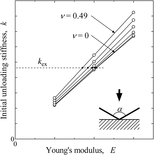
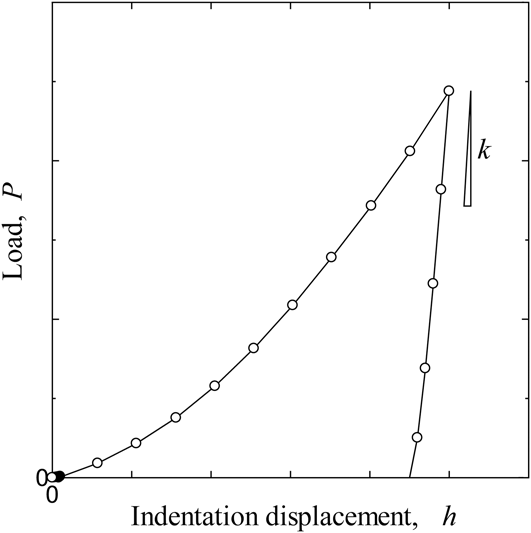
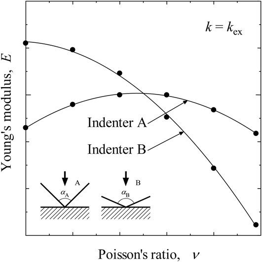
To determine the Young's modulus and Poisson's ratio by the FEM, a technique proposed by Akatsu et al. Reference Akatsu, Demura, Shinoda and Wakai11 was adopted. The technique utilizes two conical indenters with different apex angles. Using the load–displacement curves obtained by FEM analysis and the two indenters, the inclinations k in the early stages of unloading are obtained for every Young's modulus and Poisson's ratio, and the linear relationship between k and E for each of the conical indenters is derived for each Poisson's ratio. Figure 3 is a schematic diagram of the relationship between k and E for a certain value of ν and for an indenter shape and indentation displacement. A database can thus be prepared for determining E and ν. The database contains the relationship between k and E for given values of ν. The least squares method is used to approximate the relationship to a straight line that passes through the origin. By conducting two indentation tests using the two different indenters, two k ex values can be obtained, and the values of E and ν that simultaneously satisfy k = k ex for the two indenters are determined. Solid marks shown in Fig. 3 are the determined E and ν. Figure 4 is a schematic P–h diagram, and also shows k. Figure 5 is a schematic diagram of the relationship between E and ν for the two values of k ex obtained from the relationship shown in Fig. 3. The intersection of the two curves obtained by the two indenters (A and B) gives the values of E and ν. If the two curves are similar, the intersection point would be significantly altered by slight errors in the curves, which makes the determined values of E and ν liable to large errors.
Schematic diagram of the relationship between k and E for ν.

Schematic diagram of the P–h curve and k.

Schematic diagram of the relationship between Young's modulus and Poisson's ratio for k ex.

Another disadvantage of this method is that it requires two indenters of different shapes and two indentation points. In the presently proposed method, the mechanical properties can be determined without changing the indenter but by using two different load–displacement (P–h) relationships. One P–h relationship is based on the radius of the curvature of the spherical tip of the conical indenter and is for small displacements (h 1) that do not exceed the height of the spherical part of the indenter h 0. The other P–h relationship is for displacements (h 2) that are sufficiently large such that the curvature of the spherical tip of the conical indenter can be ignored. This method enables the production of multiple indents at the same point, thereby facilitating the determination of the mechanical properties at any specific point.
C. Method for determining the yield strength and work hardening factor
To determine the yield strength and work hardening factor, a part of the method proposed by Bouzakis and Michailidis Reference Bouzakis and Michailidis12 was adopted. The method involves the transformation of a load–displacement diagram obtained by experiment to a stress–strain diagram using FEM analysis.
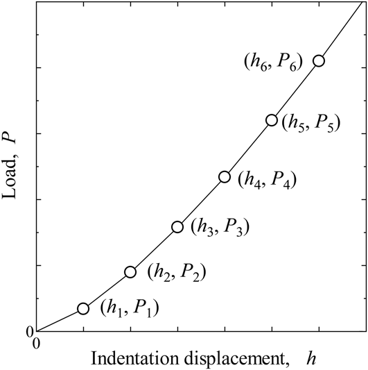
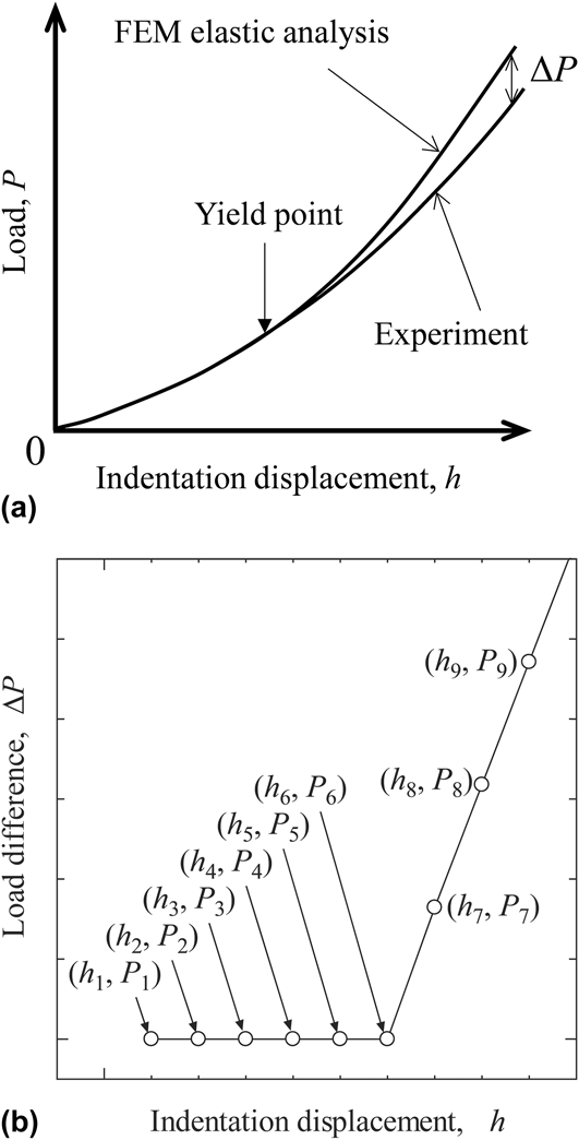
Several (h, P) points are plotted on the load–displacement graph using the results of an indentation test, as shown in Fig. 6. An FEM elastic analysis is then performed using the values of E and ν determined by the proposed method in Sec. II. B, and the load P FEM is obtained for a given h. ΔP is then calculated using ΔP = P FEM − P for the same value of h, and the relationship between ΔP and h is obtained. If (h, ΔP) is sufficiently small, the deformation of the specimen material would be elastic. However, at the elastic/plastic boundary, ΔP becomes large and there is a knee point in the relationship between ΔP and h, with a consequent change in the slope. Figure 7 shows the definition of ΔP and the schematic diagram of the ΔP–h diagram. The knee point (h 6, P 6) in Fig. 7(b) is the yield point. An FEM elastic analysis using the indentation displacement h 6 in Fig. 7 is then used to obtain the yield strength σY as the maximum equivalent stress of the specimen material.
Schematic diagram of the relationship between load and indentation displacement for some Poisson's ratio.

ΔP to determine yield strength and its definition. (a) Schematic diagram for ΔP definition. (b) Schematic diagram of relationship between ΔP and h.

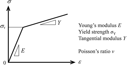
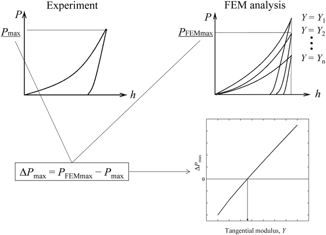
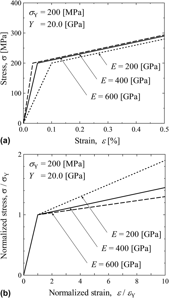
An FEM analysis using the obtained values of E, ν, and σY is then used to determine the work hardening factor n based on the relationship between n and ΔP max (ΔP max = P maxFEM − P max). P max is the load P at the maximum indentation displacement h max. In this study, a measurement method was proposed, and then considering its fast convergence of the FEM analysis, a material that has simple properties was used as an example. The stress–strain diagram of the specimen material was simply approximated by two straight lines, and the tangent modulus Y after the yield point was determined instead of n. Figures 8 and 9, respectively, show the stress–strain diagram and ΔP max–Y diagram.
S–S diagram.

Schematic diagram of the relationship between ΔP max and Y.

III. ANALYTIC MODEL
The indentation analyses were performed using an axial symmetry model and the general-purpose finite element program ANSYS 15.0. Axial symmetry triangle six-node elements were used and the coefficient of friction on the contact surface was set to zero, because there is no significant influence of friction if α is 120°. Reference Bucaille, Stauss, Felder and Michler10 Mata and Alcalá Reference Mata and Alcalá22 focused on pile-up or sink-in around the contact boundary, and concluded that the actual coefficient of friction has to be taken into account in the assessment of mechanical properties, specially in such solids exhibiting a pile-up effect. If α is smaller, the pile-up effect is easier to occur. Reference Dugdale23 Then the conclusion of Mata and Alcalá Reference Mata and Alcalá22 corresponds to that of Bucaille et al. Reference Bucaille, Stauss, Felder and Michler10 And Lee et al. Reference Lee, Kim and Lee24 who discussed the friction effect on load–depth relation for the spherical indenter and found that if the ratio of depth to diameter is small, it is insensitive. Assuming a rigid body, the mechanical properties of the indenter were set to E i = 200 TPa and νi = 0.30, and the apex angle α was set to be 120°. The Young's modulus of the indenter was sufficiently large compared to that of the specimen material. The curvature radius of the tip of the indenter ρ was set to be 4 μm, as a feasible size in real calculations. Based on the geometry of the indenter, the displacement h 0 which is shown in Fig. 1 for the spherical indenter is h 0 ≅ 0.54 μm. Although the concrete ρ value is small, the numerical results will be made useful with the dimensionless expression. To be meaningless of the concrete ρ value (4 μm), h 0 was used for the dimensionless expression to the indentation depth. In the results shown later, when dimensionless expression to the indentation depth h/h 0 is used, then the concrete ρ value (4 μm) is meaningless. h 0 becomes fixed automatically with the combination of the apex angle α and the indenter tip curvature radius ρ.
To determine the mechanical properties of the specimen material from the database, E and ν were assumed to be within 200–600 GPa and 0.0–0.49, respectively, and σY was fixed to be 200 MPa and Y to 20.0 GPa. Figure 10(a) shows the stress–strain relation used for the analyses. The relation was normalized by σY and εY (=σY/E), and Fig. 10(b) shows the normalized stress–strain relationship. The relationship depends only on Y/E. When the analytical stress components and strain components are normalized by σY and εY, respectively, the normalized components depend on Fig. 10(b). Therefore, the stress and strain obtained in this study by using the fixed σY and Y can be converted to stress and strain by using another σY and Y, when Y/E is the same. The loading procedure was as follows. The indenter was initially used to produce the indent until the displacement h 1 was 0.1 μm (≅0.187 h 0), after which it was unloaded until it was free from the specimen surface. It was then reloaded until the displacement h 2 was 5 μm (≅9.33 h 0), and again unloaded until it was free from the specimen surface. Therefore, the spherical part of the indenter was used for the first indent, and the conical part of the indenter was used for the second indent. From the procedure, k 1 from h 1 and k 2 from h 2 were obtained.
Stress–strain relation used in this study. (a) Stress–strain relation. (b) Normalized stress–strain relation.

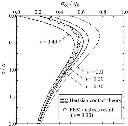
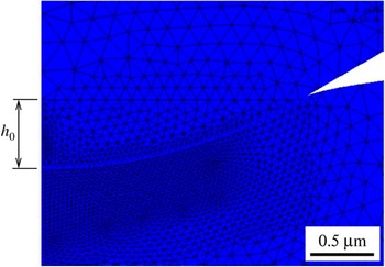
Figure 11(a) shows the analysis model and the boundary conditions. The indenter and the specimen were modeled in consideration of axial symmetry. The number of the elements was 9,323 and the number of the nodes was 18,616. The element size was the minimum around the tip of the indenter and its contact with the specimen because stress concentration is generated around the contact point. The minimum element size was about 39 nm. The validity of the meshing will be discussed later using Fig. 12 comparing with the Hertzian contact theory. A finer meshing around the contact area was used only for Fig. 18 to obtain accurate maximum equivalent stress, because the equivalent stress around the contact point is distributed. The number of the elements was 26,124 and the number of the nodes was 52,283. The minimum element size was about 0.26 nm. The validity of the finer meshing will be discussed later using Fig. 18(b). Figure 12 shows the relationship between the distance (z) from the contact point and the equivalent stress (σeq) derived from Hertzian contact theory. Reference Johnson17 The distance was normalized by the contact radius (a) and the equivalent stress was normalized by the maximum contact pressure (q 0). A steep stress variation is generated just beneath the contact point, and to represent the stress variation and accurate analysis, the element division of FEM analysis was determined as shown in Fig. 11. To check the validity of the element division, elastic analysis using the analysis model was performed. The used material properties and the load were the elastic element of the material properties used later (E = 200 GPa, ν = 0.30) and the smaller displacement h 1 (h 1/h 0 = 0.187), respectively. The analysis result is shown in Fig. 12 as open marks. The open marks are nodal solution results. From Fig. 12, the analysis results seem to represent the stress variation well and the element division was considered as valid.
Analysis model and boundary conditions. (a) Whole model and boundary conditions. (b) Around the indentation tip. (c) Detail of the indenter tip.

Equivalent stress distribution in the depth direction (q 0: maximum contact pressure).

For the analysis to determine σY, another element division was used because the indentation displacement was extremely smaller than that of the other analysis, and the validity of the element division will be checked with the analysis results later.
IV. ANALYSIS RESULTS
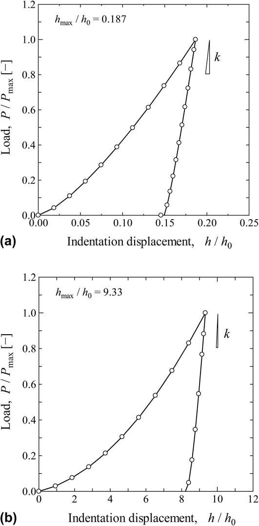
The mechanical properties determined by the method proposed in this paper were verified by comparison with the known properties of the material. The known mechanical properties determined by the proposed analyses using the P–h diagram are E ex = 200 GPa, νex = 0.30, σYex = 200 MPa, and Y ex = 20.0 GPa. Hereafter, the value of k determined from the P–h diagram with known mechanical properties is denoted by k ex for the experimental result. Figure 13 shows the P–h diagram obtained by FEM analysis, and Fig. 14 shows the contact conditions for h 1/h 0 = 0.187 and h 2/h 0 = 9.33. From Fig. 14, it can be seen that only the spherical part of the indenter made contact for h 1/h 0 = 0.187, whereas both the spherical and conical parts made contact for h 2/h 0 = 9.33.
P–h curves simulated with FEM. (a) h 1/h 0 = 0.187 (h 1 = 0.1 μm). (b) h 2/h 0 = 9.33 (h 2 = 5 μm).

FEM analysis result. (a) h 1/h 0 = 0.187 (h 1 = 0.1 μm). (b) h 2/h 0 = 9.33 (h 2 = 5 μm).

A. Determined Young's modulus and Poisson's ratio
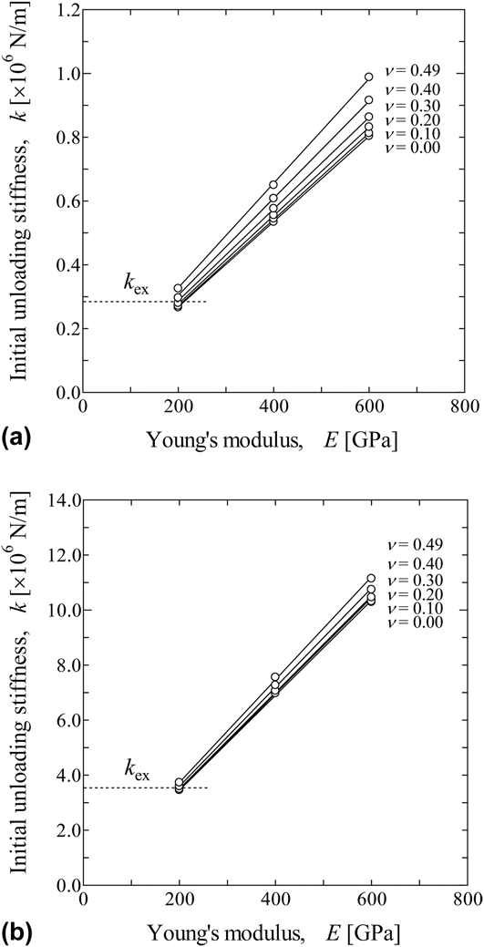
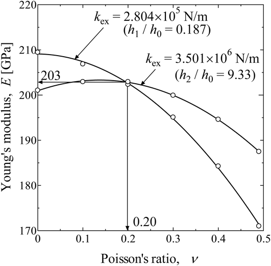
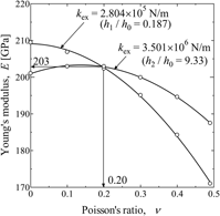
Figure 15 shows the relationship between k and E for Poisson's ratios of 0.0, 0.10, 0.20, 0.30, 0.40, and 0.49, respectively. In Fig. 13, k ex = 2.804 × 10⁵ N/m for h 1/h 0 = 0.187, and k ex = 3.501 × 10⁶ N/m for h 2/h 0 = 9.33. Figure 16 shows the values of E and ν that were determined using Fig. 15 for k = 2.804 × 10⁵ N/m (h 1/h 0 = 0.187) and k = 3.501 × 10⁶ N/m (h 2/h 0 = 9.33). Figure 16 shows that the relationship between E and ν for indentation displacements of h 1 and h 2 that are different as expected. The analysis results for each k were fitted by the quadratic function. From the intersection of the two curves in the figure, it is determined that E = 203 GPa and ν = 0.20.
Relationship between k and E for ν. (a) h 1/h 0 = 0.187 (h 1 = 0.1 μm). (b) h 2/h 0 = 9.33 (h 2 = 5 μm).

Relationship between Young's modulus and Poisson's ratio for k.

B. Determined yield strength and work hardening factor
Figure 17 shows the FEM analysis results of the yield strength determined from the knee point. Figure 17(a) shows the relationship between load difference and indentation displacement obtained from the P–h diagram in Fig. 13(b) by FEM elastic analyses using E = 203 GPa and ν = 0.20 (the values obtained in Sec. IV. A). The load difference ΔP was normalized by FEM analyzed value P FEM and the indentation displacement h was normalized by h 0. The knee point at which the slope of the relationship between ΔP and h changes in Fig. 17(a) is around h/h 0 = 4 × 10⁻⁵, which shows that the result of the elastic analysis is different from that of the experiment. Although the accuracy of the knee point directly affects the accuracy of the determined yield strength, detailed FEM analyses were performed using values of h/h 0 between 3 × 10⁻⁵ and 5 × 10⁻⁵. Figure 17(b) shows the result. The relationship between ΔP/P FEM and h/h 0 does not show smoothness because of the discretization error of the FEM analyses. As shown in Fig. 7(b), ΔP/P FEM is theoretically constant when h/h 0 is smaller than knee point. Therefore, as a point for which ΔP/P FEM begins to rise certainly, h/h 0 = 3.96 × 10⁻⁵ was selected where the knee point was found to occur.
FEM analysis results for determination of the knee point which indicates yield strength. (a) Relationship between ΔP/P FEM and h/h 0. (b) Detailed relationship between ΔP/P FEM and h/h 0.

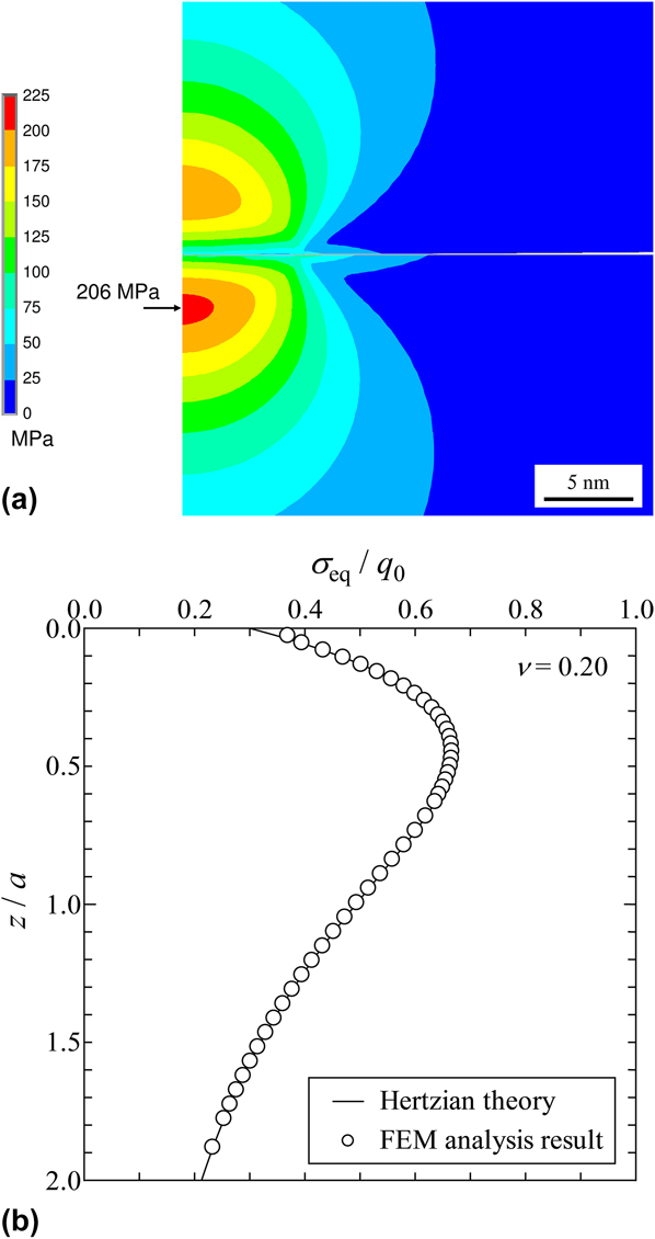
Figure 18(a) shows the equivalent stress distribution and maximum equivalent stress around the contact point. The stress was determined by FEM analysis for h/h 0 = 3.96 × 10⁻⁵. The indenter shape is spherical, and the specimen shape is flat before the contact. The radius of the curvature of the indenter is large enough comparing with the indent depth. Then the radii of the curvature of the indenter and the specimen can be regarded approximately to be the same, and the contact can be regarded as approximately two spheres contact. The contact pressures are the same from the law of action and reaction. Then, assuming the Hertzian contact theory, Reference Johnson17 the equivalent stress depends on the Poisson's ratio only Reference Johnson17 as shown in Fig. 12, and the maximum equivalent stress appears slightly below the contact point. Reference Davies25 The analysis shown in Fig. 18 was performed under the conditions of νi = 0.30 for the indenter and ν = 0.20 for the specimen. Then, the equivalent stress distribution of the indenter is different from that of the specimen. Therefore, there is a 2-fold symmetry for the equivalent stress distribution of the indenter and the specimen, and the distribution is not symmetric. A yield strength σY of 206 MPa was determined for the specimen based on the maximum equivalent stress of 206 MPa under the applied conditions. Figure 18(b) shows the equivalent stress distribution of the specimen from the contact point. z is the distance from the contact point to the inside of the specimen. The analysis results seem to represent the stress variation well and the element division for this analysis was considered as valid.
Equivalent stress distribution and the maximum equivalent stress from FEM analysis. (a) Equivalent stress distribution and maximum equivalent stress. (b) Equivalent stress distribution in the depth direction.
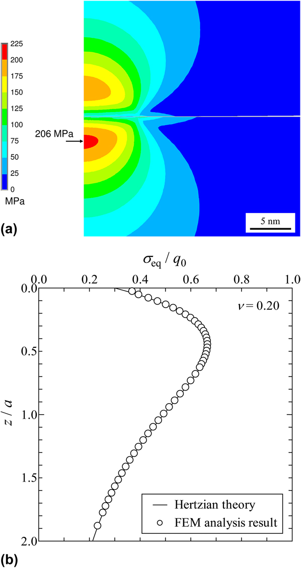
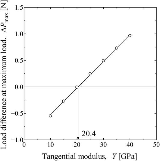
Figure 19 shows the relationship between ΔP max as obtained from the maximum experimental indentation displacement h 2/h 0 = 9.33 and various values of Y. A tangential modulus Y of 20.4 GPa was obtained from ΔP max = 0.
Relationship between ΔP max and Y.

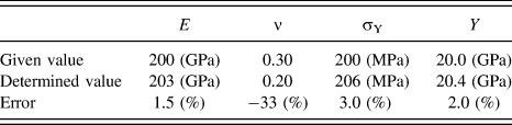
It was thus determined that E = 203 GPa, ν = 0.20, σY = 206 MPa, and Y = 20.4 GPa. Table I shows the errors in the analytically determined mechanical properties compared to the known values.
Determined value errors from given mechanical properties.

C. Errors in the Young's modulus and Poisson's ratio
A comparison of the mechanical properties determined by the proposed method with the known values of E ex = 200 GPa and νex = 0.30 reveals that the error in the Poisson's ratio is large compared to that in the Young's modulus. This can be attributed to the dependency of k on the Young's modulus being significantly different from that of the Poisson's ratio. That is, as shown in Fig. 15, when the variation of the Young's modulus with k for a given Poisson's ratio is compared with the variation of the Poisson's ratio with k for a given Young's modulus, the latter is significantly greater. Therefore, considering that the Young's modulus and Poisson's ratio were determined based on k in this study, if k varies from the true value, the error in the Young's modulus could be relatively small, whereas that in the Poisson's ratio would be relatively large. For this reason, it is supposed that a slight error in k due to an FEM analysis discretization error caused a relatively large error in the Poisson's ratio.
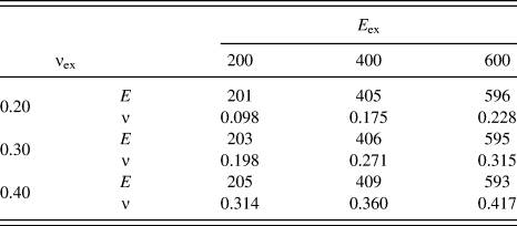
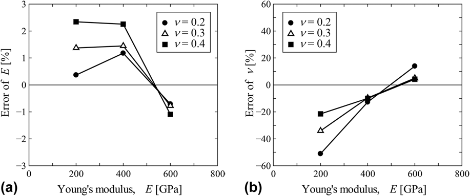
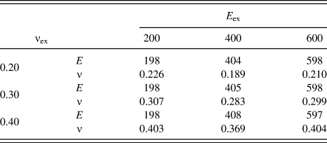
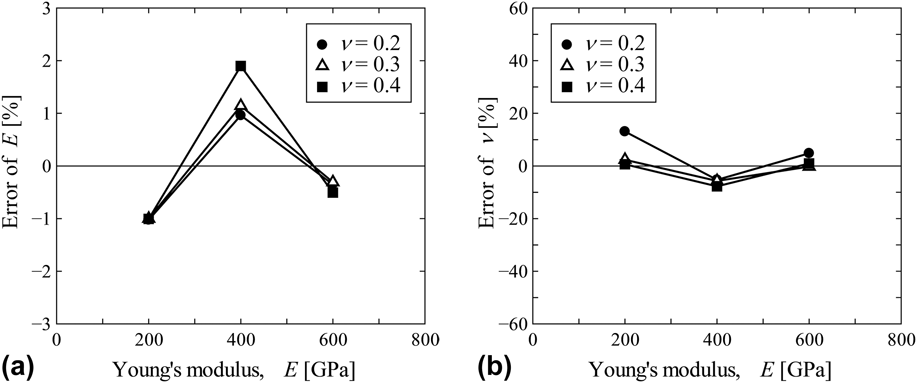
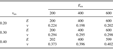
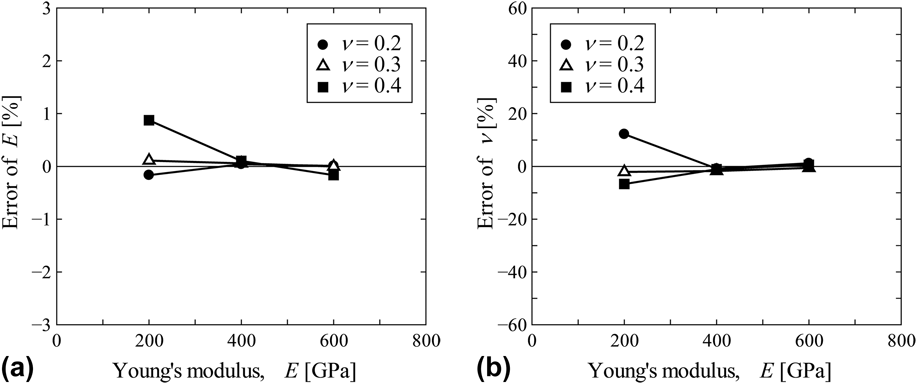
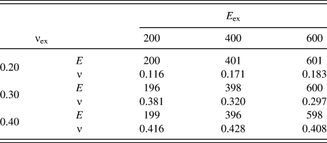
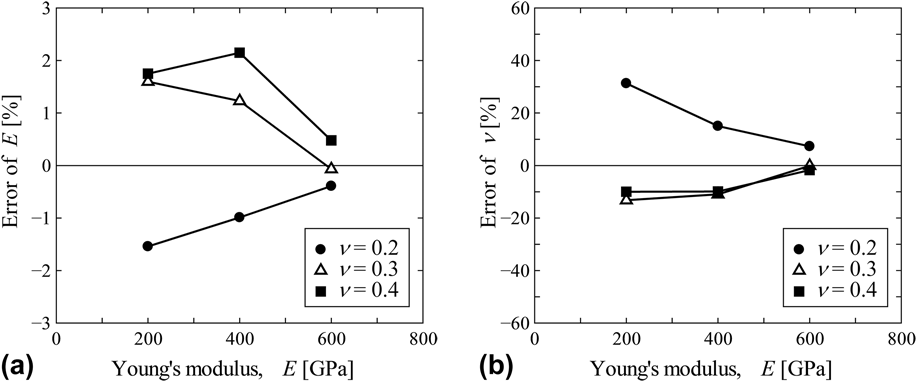
To confirm the cause of the observed error, error analyses were performed. First, FEM analyses were performed to obtain k ex for various mechanical properties, namely, E ex = 200, 400, and 600 GPa, and νex = 0.20, 0.30, and 0.40. Based on the obtained values of k ex, the proposed method was used to determine the mechanical properties. The errors are compared in Table II. It can be seen that the errors in the Poisson's ratio are relatively large and that they are not dependent on the mechanical properties. Figure 20 shows the errors in the results with respect to the original values of the Young's modulus and Poisson's ratio. The figure reveals that the errors in the Young's modulus and Poisson's ratio were small around E = 500 GPa. This suggests that the errors originated from the approximations of the data in Fig. 15. The approximation of the relationship between k and E was thus changed from a linear function that passes through the origin into a general linear function. Table III and Fig. 21 show the errors in the values of E and ν after the change, and it can be seen that the errors were reduced. Furthermore, Fig. 21 shows that the errors in the Young's modulus and Poisson's ratio were less around E = 300 and 550 GPa. This can once again be attributed to the approximations in the database, and the approximation method was further changed from a linear function to a quadratic function. Table IV and Fig. 22 show the errors in the determined values of E and ν after the second change. It can be seen that the errors were further reduced. Hence, by careful data approximation, it was possible to reduce the error in the determined Young's modulus to less than 1%, and that in the Poisson's ratio to less than 15%. Table IV and Fig. 22 show the sensitivity to a variation in E, too. The P–h curve is dependent on E, and then the error analysis to the difference in E is considered to be equivalent to the sensitivity analysis to the P–h curve.
Calculation results of E and ν by using a proportional approximation for Fig. 15.

Relationship between error and E by using a proportional approximation for Fig. 15. (a) Error of E. (b) Error of ν.

Calculation results of E and ν by using linear function approximation for Fig. 15.

Relationship between error and E by using linear function approximation for Fig. 15. (a) Error of E. (b) Error of ν.

Calculation results of E and ν by using quadratic function approximation for Fig. 15.

Relationship between error and E by using quadratic function approximation for Fig. 15. (a) Error of E. (b) Error of ν.

V. DISCUSSION
A. Error caused by the indentation displacement
In this study, a single indenter with a special shape was used to produce two indentation displacements to determine the mechanical properties of the specimen material. The first displacement h 1/h 0 = 0.187 was produced when only the spherical part of the indenter made contact with the specimen, and the second displacement h 2/h 0 = 9.33 was produced by the spherical and conical parts. The errors in the obtained results are supposed to be the maximum for an indentation displacement produced at the time of transition between the spherical and conical parts of the indenter. In this case, error analyses of the determined mechanical properties were performed.
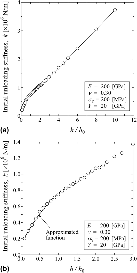
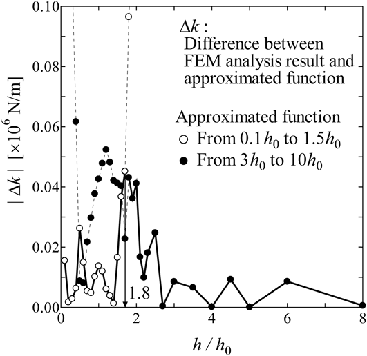
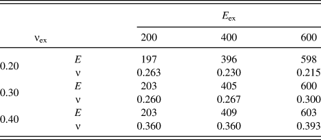
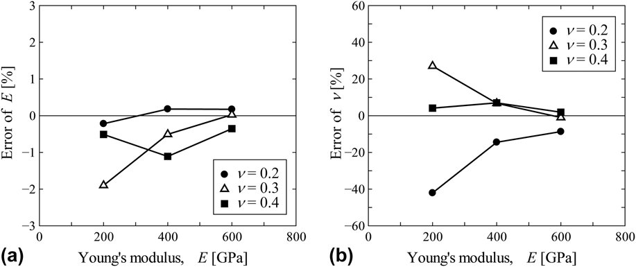
The k values of indentation displacements between h/h 0 = 0.1 and 10 were analyzed by FEM analyses. As noted earlier, the h 0 displacement at the time of transition is between the spherical and conical parts of the indenter. The material properties used in this FEM analyses were E = 200 GPa, ν = 0.30, σY = 200 MPa, and Y = 20.0 GPa. The obtained relationship between k and h/h 0 shown in Fig. 23 is supposed to correspond to a spherical indenter for small values of h/h 0, and to a conical indenter with a small spherical tip for large values of h/h 0. Because some parts of the spherical part of the indenter is not in contact with the specimen for an indentation displacement of h/h 0 = 1, h/h 0 = 1 cannot be considered to correspond to the transition between the spherical and conical parts of the indenter. The deformed conditions used for the FEM analyses for different indentation displacements were therefore used to confirm the actual contact conditions. Figure 24 shows the contact condition for an indentation displacement of h/h 0 = 1.5. In this case, the entire spherical part of the indenter (of length h 0) was observed to make contact with the specimen, and it can be assumed that the indent was a spherical indent. Hence, considering the indentation displacement of h/h 0 = 1.5 to correspond to the transition from a spherical indenter to a conical indenter, the relationships between k and h in the ranges of h/h 0 = 0.1–1.5 and h/h 0 = 3.0–10 were approximated by quadratic functions. The absolute differences between the k values shown in Fig. 23 and those obtained by the approximated relationship were then calculated. Figure 25 shows the results. It can be seen that the maximum error occurs at h/h 0 = 1.80. The previously presented mechanical properties were those determined using h 1/h 0 = 0.187 and h 2/h 0 = 9.33. The indentation displacements were then changed to h 1/h 0 = 0.187 and h 2/h 0 = 1.80, and then to h 1/h 0 = 1.80 and h 2/h 0 = 9.33. The mechanical properties determined from the k values obtained using these pairs of indentation displacements were then compared with the given mechanical properties of the specimen material. The observed errors are given in Tables V and VI and Figs. 26 and 27. It can be seen that the errors in the Young's modulus and Poisson's ratio obtained by the proposed method are less than 3 and 45%, respectively. In other words, the worst case in the errors of Young's modulus and Poisson's ratio are 3 and 45%, respectively.
k dependency on indentation displacement. (a) h/h 0 = from 0.1 to 10. (b) Detail of low h/h 0.

Analysis result with h/h 0 = 1.5.

Difference between the approximate equation and experimental value.

Calculation results of E and ν by using h 1/h 0 = 0.187 and h 2/h 0 = 1.80.

Calculation results of E and ν by using h 1/h 0 = 1.80 and h 2/h 0 = 9.33.

Relationship between error and E by using h 1/h 0 = 0.187 and h 2/h 0 = 1.80. (a) Error of E. (b) Error of ν.

Relationship between error and E by using h 1/h 0 = 1.80 and h 2/h 0 = 9.33. (a) Error of E. (b) Error of ν.

B. Discretization error of FEM analysis
The effect of the discretization error of the FEM analysis on the determined mechanical properties is worth mentioning.
The elastic contact area in this study was round, and its diameter is denoted by D. From Eq. (3), its area is given by
 $$A = {\left( {k{{\sqrt \pi } \over 2}{{1 - {\nu ^2}} \over E}} \right)^2}\quad .$$
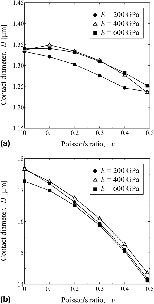
D was thus calculated for the values of A obtained by using Eq. (5) and the k values determined are by the FEM analyses results shown before. Figure 28 shows the relationship between D and ν for the two indentation displacements and three values of E. For the large indentation displacement [Fig. 28(b)], the relationships between D and ν for the three E values are almost the same, and analyses containing little error can be considered to have been achieved. However, for the small indentation displacement [Fig. 28(a)], the relationships between D and ν for the three E values were significantly different. This can be attributed to the discretization error because, for a small indentation displacement, the size of the element relative to the deformation is large, thereby increasing the relative error.
Relationship between D and ν. (a) h 1/h 0 = 0.187. (b) h 2/h 0 = 9.33.

VI. CONCLUSION
In this study, a method for determining the mechanical properties (Young's modulus, Poisson's ratio, yield strength, and work hardening factor) at specific points of a material based on the relationship between the indentation load and displacement using an inverse problem analytic method and finite element analysis was developed and verified. The indenter used for the proposed method combines the characteristics of spherical and conical indenters and can be used to produce multiple indents at the same point in a specimen material. Detailed precision verifications of the properties determined by the proposed method were performed, and following results were found for the element meshing shown in Fig. 11. In the ideal case, that is by using the spherical part and the conical part of the indenter, by using indentation depths h 1/h 0 = 0.187 and h 2/h 0 = 9.33, the Young's modulus, Poisson's ratio, and yield strength could be determined with errors of less than 1, 15, and 3%, respectively. In the worst case, that is by using the transition indentation depth between the spherical part and the conical part of the indenter, by using indentation depths h 1/h 0 = 0.187 and h 2/h 0 = 1.80 or by using h 1/h 0 = 1.80 and h 2/h 0 = 9.33, the Young's modulus and Poisson's ratio could be determined with errors of less than 3 and 45%, respectively.