1. Introduction
In nature, wind waves of all scales are asymmetric both with respect to the horizontal and vertical axes. The front–back (or fore–aft) asymmetry, i.e. the asymmetry with respect to the vertical axis, manifests itself in statistically steeper front slopes. Understanding and faithful modelling of this asymmetry for the waves of the gravity–capillary range is important for remote sensing (e.g. Valenzuela Reference Valenzuela1978; Chapron et al. Reference Chapron, Kerbaol, Vandemark and Elfouhaily2000), since the backscattering of microwaves by capillaries strongly depends on the angle of the scattering facet, to which the front–back asymmetry makes a noticeable contribution. Thus, the front–back asymmetry of wave crests is an important characteristic of sea surface that cannot be retrieved from the spectral density of waves. It may be linked to wave breaking (Chapron, Vandemark & Elfouhaily Reference Chapron, Vandemark and Elfouhaily2002), which impacts air–sea exchange of gas, heat and momentum. Wind–wave interaction might also depend on specific shape of wave crests (e.g. Jeffreys Reference Jeffreys1925; Csanady Reference Csanady1985), and some field and numerical experiments suggest that wind energy input depends on the front–back asymmetry of waves (Agnon et al. Reference Agnon, Babanin, Young and Chalikov2005), which is explained by the air-flow separation.
In the seminal works by Cox & Munk (Reference Cox and Munk1954, Reference Cox and Munk1956) the overall sea surface slope statistics for various wind conditions was inferred from photographs of sun glitter patterns; the Gram–Charlier expansion was used to quantify the non-Gaussian features of the probability density function of slopes. The physical mechanisms of the skewness of the wave slope distribution observed in Cox & Munk (Reference Cox and Munk1956) were discussed by Longuet-Higgins (Reference Longuet-Higgins1982). Two possible explanations were considered: (i) the skewness of the slope distribution could be associated with the front–back asymmetry of individual waves, produced by the bound second harmonic appropriately phase shifted, or, (ii) the skewness could be originating from a simple slope addition, when a wavetrain of short capillaries is modulated in phase with the slope of a longer wave. It was found that neither wind stress nor viscous damping can produce a phase shift in the second harmonic large enough to match the observed skewness of the slope distribution; the slope addition mechanism was viewed as a more plausible explanation. However, Munk (Reference Munk2009) argues that if, according to the slope addition hypothesis, parasitic capillary ripples were responsible for the skewness, they would also make a corresponding contribution to the mean-square slope, which does not agree with the field measurements. Thus the question remained open.
To quantify the front–back asymmetry in observations two equally legitimate approaches are commonly used. The first approach applies to individual waves and requires direct measuring of the wave geometrical characteristics, such as the position of a crest with respect to the two nearest troughs (e.g. Bailey, Jones & Toba Reference Bailey, Jones and Toba1991; Babanin et al. Reference Babanin, Chalikov, Young and Savelyev2010; Banner et al. Reference Banner, Barthelemy, Fedele, Allis, Benetazzo, Dias and Peirson2014). The shortcoming of this approach is that it is not particularly suitable for analysis of long data records, since it requires explicit decomposition of the wave field into a series of individual crests and an analysis of each crest. The second commonly used approach is a by-product of bi-spectral analysis. It was noted by Masuda & Kuo (Reference Masuda and Kuo1981) that imaginary part of bi-spectra can be used to characterise the wave front–back asymmetry. The corresponding third moment can also be computed directly from the Hilbert transform of the wave profile (Elgar Reference Elgar1987). The link between the bi-spectral properties of shoaling waves and front–back asymmetry of their profiles is demonstrated in Elgar & Guza (Reference Elgar and Guza1985). The same definition of asymmetry was employed in experimental studies of short wind waves by Leykin et al. (Reference Leykin, Donelan, Mellen and McLaughlin1995) for waves of the short gravity range and in Zavadsky & Shemer (Reference Zavadsky and Shemer2017) for gravity–capillary waves, which also yielded the dependence of asymmetry on wind speed.
However, despite the considerable progress in accumulation of data, the physical mechanisms of asymmetry have not been identified yet. Possible mechanisms include wave breaking and strong wind forcing (Fedorov & Melville Reference Fedorov and Melville2009). Laboratory experiments by Leykin et al. (Reference Leykin, Donelan, Mellen and McLaughlin1995) and Zavadsky & Shemer (Reference Zavadsky and Shemer2017) were conducted for the range of wind speeds where wave breaking is likely to be essential.
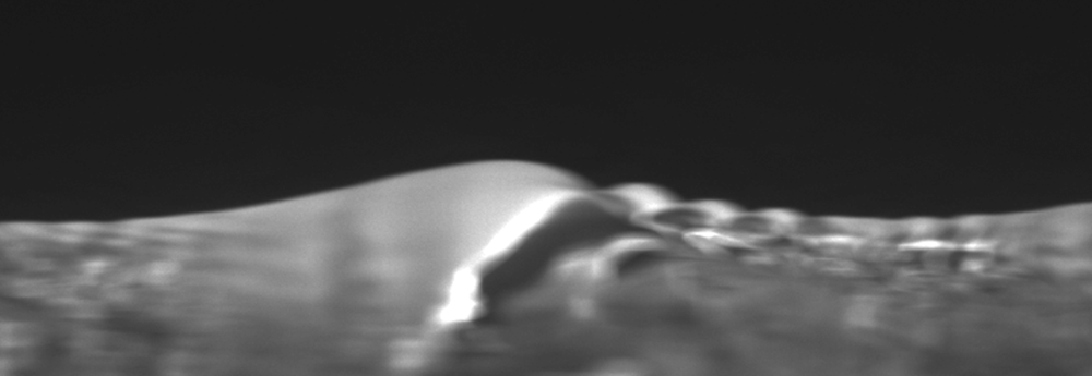
Here, we focus our study on non-breaking waves of the gravity–capillary range. Steep waves of this range generate short capillary ripples on their crests due to the phase synchronism (Munk Reference Munk1955; Longuet-Higgins Reference Longuet-Higgins1995). The capillary waves are so rapidly decaying due to viscous damping that the parasitic ripples usually propagate only a fraction of the primary wavelength forming a well-defined wavetrain. The group velocity of capillary waves is always greater than their phase velocity. Recall that the parasitic capillaries generated at the crest via Longuett–Higgins resonance with the phase velocity equal to that of the crest propagate forward with the group velocity until, at a certain distance from the crest, they are suppressed by viscosity. Therefore, the train of parasitic capillaries is always localised on the forward face of the primary wave. Although our numerical model allows us to reproduce the initial stages of spilling breaker development, we restrict our study to the range of scales where such processes are dominated by surface tension forces (Duncan Reference Duncan2001). Formation of asymmetric gravity–capillary wave patterns was observed in numerical simulations by Fedorov & Melville (Reference Fedorov and Melville1998) and Hung & Tsai (Reference Hung and Tsai2009), but the phenomenon of asymmetry itself was not studied. Laboratory experiments focussed on dissipation mechanisms of wind generated gravity–capillary waves by Caulliez (Reference Caulliez2013) have identified the parameter range where wave breaking and microbreaking do not occur, while the wave profiles in this range exhibit pronounced asymmetry and characteristic parasitic capillary wavetrains on the front slope (see figures 4–6 there or figure 1 taken from Caulliez Reference Caulliez2013). Thus, although wave breaking might be an important factor in making the waves asymmetric, the point we stress here is that pronounced asymmetry can exist without wave breaking, as shown by Caulliez (Reference Caulliez2013) and illustrated by figure 1.
An example of a longitudinal cross-section of a wave profile observed at the Luminy ‘Large Air-Sea Interaction Facility’ as viewed from the side by the camera. The  $5.0\ \mathrm {m\ s^{-1}}$ wind is blowing from left to right, the fetch is
 $6\ \mathrm {m}$, the characteristic wavelength is
 $6\ \mathrm {cm}$. There are no wave breaking in this regime (according to the classification proposed in Caulliez (Reference Caulliez2013) it is ‘regime II’. The photo is courtesy of G.Caulliez).

Our aim is to identify mechanisms of front–back asymmetry of non-breaking gravity–capillary waves and to study how it depends on parameters.
To model properly the evolution of strongly nonlinear gravity–capillary waves in the ocean is a formidable challenge; it is necessary to take into account three-dimensionality of wave field, vorticity strongly localised near the surface, turbulence in the water, interaction with longer waves, air entrainment and complex interaction with the turbulent wind, which includes the formation of spray. At present, such an ambitious undertaking is far beyond the art of the possible. There are works which tackle some aspects of the listed elements, for example, viscous decay due to molecular viscosity (Fedorov & Melville Reference Fedorov and Melville1998), generation of vorticity at the free surface (Hung & Tsai Reference Hung and Tsai2009), exact three-dimensional simulation of the Navier–Stokes equations in the absence of wind and turbulence (Hung & Tsai Reference Hung and Tsai2009), interaction of waves with a turbulent surface layer (Fedorov & Melville Reference Fedorov and Melville2009) and the generation of spay (Troitskaya et al. Reference Troitskaya, Kandaurov, Ermakova, Kozlov, Sergeev and Zilitinkevich2018).
Here, for a study focussed on the single issue of the nature of the wave asymmetry, we, as a first step, adopt the simplest possible approach enabling us to capture the essence of the phenomenon: we consider the dynamics of potential strongly nonlinear strictly two-dimensional gravity capillary waves approximately taking into account viscosity and mimicking the effect of wind. We validate our approach a posteriori by comparison with a more accurate model of Fedorov & Melville (Reference Fedorov and Melville1998) and direct numerical simulations of the Navier–Stokes equations by Hung & Tsai (Reference Hung and Tsai2009).
The paper is organised as follows. The physical model employed in our simulations, and parameterisations of wind forcing and viscous effects are described in § 2. Section 3 provides details of the set-up and describes how our results compare with other models that take more accurate account of viscous effects: the Navier–Stokes equations without wind by Hung & Tsai (Reference Hung and Tsai2009) and the approximate model of Fedorov & Melville (Reference Fedorov and Melville1998).
Alternative methods of quantifying the profile asymmetry and their robustness, as well as the physical mechanism of asymmetry, are discussed in § 4. In § 5 we study how asymmetry of the mean wave profile depends on parameters of the primary wave. In the concluding § 6, we summarise our findings and discuss how asymmetry may be affected by other factors that we did not take into account, such as, e.g. interaction with longer waves, microbreaking or the presence of surface films. We also briefly discuss the available experimental data and the new insight they provide into the physical mechanisms of asymmetry.
2. Basic equations and assumptions
We confine our study to the evolution of two-dimensional steep gravity–capillary waves. We consider motions of unit density fluid with a continuous free surface assuming the motions to be potential to leading order. To take into account viscous dissipation the classical potential motion model is modified in the spirit of Ruvinsky, Feldstein & Freidman (Reference Ruvinsky, Feldstein and Freidman1991) and Longuet-Higgins (Reference Longuet-Higgins1992).
In the classical setting, the velocity potential  $\varphi$ satisfies the Laplace equation
 \begin{equation} {\rm \Delta}\varphi=0, \end{equation}
in the two-dimensional fluid domain confined between the free surface and the bottom. We employ the Cartesian coordinate frame  $(x,y)$ with the
 $x$ axis coinciding with the unperturbed water surface. The kinematic and dynamic boundary conditions at the free surface
 $y=\eta (x,t)$ are expressed in terms of
 $\varphi$ and
 $\eta$
 \begin{gather} \frac{\partial\eta}{\partial t} + \frac{\partial\varphi}{\partial x}\frac{\partial\eta}{\partial x} - \frac{\partial\varphi}{\partial y} = 0, \end{gather}
 \begin{gather}\frac{\partial\varphi}{\partial t} + \frac{|\boldsymbol{\nabla}\varphi|^2}{2} + g\eta + p - T\varkappa = 0, \end{gather}
 \begin{gather}\varkappa = \frac{\eta_{xx}^{\prime\prime}}{(1+\eta_x^{\prime 2})^{3/2}}, \end{gather}
where  $g$ is the acceleration due to gravity,
 $p$ is external pressure and
 $T$ is the surface tension coefficient. We confine our study to deep water, which implies the boundary condition at infinity is
 \begin{equation} |\boldsymbol{\nabla}\varphi| \to 0 \quad \text{as } y \to -\infty. \end{equation}
We introduce the full mechanical energy  $E$ of the system as
 \begin{equation} E = \int \textrm{d} x\int_{y<\eta(x)} \textrm{d} y \left( gy + \frac{|\boldsymbol{\nabla}\varphi|^2}{2} \right) + T\int \, \textrm{d} s, \end{equation}
where  $s$ is the ‘surface length’ measured along the surface profile. Hereinafter, as we consider the motion of the system to be periodic in space, we will for brevity refer to (2.6) computed per the wave period as the ‘energy’.
In contrast to most studies of free potential water waves, where pressure  $p$ is set to be constant, we use the pressure term
 $p$ to parameterise wind input and decay due to viscosity
 \begin{equation} p = p_{wind} + p_{visc}. \end{equation}
Viscous decay is modelled by the term
 \begin{equation} p_{visc} = -4\nu\frac{\partial^2\varphi}{\partial s^2}, \end{equation}
where  $\nu$ is kinematic viscosity and
 $s$ is coordinate along the surface. The exact boundary conditions for a viscous flow include stress continuity, which is, of course, impossible to satisfy for potential flows. However, by assuming the viscosity and vortical velocity components are small, the equations of quasi-potential theory for small-amplitude waves can be obtained (Ruvinsky et al. Reference Ruvinsky, Feldstein and Freidman1991)
 \begin{gather} \frac{\partial\varphi}{\partial t} + \frac 1 2 |\boldsymbol{\nabla}\varphi|^2 + g\eta + p - T\varkappa = 2\nu\frac{\partial^2\varphi}{\partial s^2}, \end{gather}
 \begin{gather}\frac{\partial\eta}{\partial t} + \frac{\partial\varphi}{\partial x}\frac{\partial\eta}{\partial x} -\frac{\partial\varphi}{\partial y} = -\frac{\partial\zeta}{\partial x}, \end{gather}
 \begin{gather}\frac{\partial^2\zeta}{\partial t\partial s} + 2\nu\frac{\partial^3\varphi}{\partial n\partial s^2} = 0, \end{gather}
where  $\zeta$ is the vortical part of the streamfunction, such that the velocity components are
 \begin{equation} v_x = \frac{\partial\varphi}{\partial x} + \frac{\partial\zeta}{\partial y}, \quad v_y = \frac{\partial\varphi}{\partial y} - \frac{\partial\zeta}{\partial x}. \end{equation}
In the linearised version of the above system each of the right-hand sides of (2.9) and (2.10) is responsible for exactly half of the overall viscous damping rate  $\gamma _{visc}$,
 \begin{equation} -\gamma_{visc} = \nu k^2 + \nu k^2, \end{equation}
where  $k$ is the gravity–capillary wave wavenumber. To avoid solving equation for
 $\zeta$ we, following Ruvinsky et al. (Reference Ruvinsky, Feldstein and Freidman1991) and Longuet-Higgins (Reference Longuet-Higgins1992), choose to parameterise viscous damping as (2.8), effectively multiplying the right-hand side of (2.9) by a factor of two while omitting the right-hand side of (2.10). Although such a parametrisation has been justified asymptotically only for small-amplitude waves, we will use parametrisation (2.8) for steep waves as well. A posteriori check by comparison with the full Navier–Stokes simulations shows that it remains meaningful for very steep wave profiles and agrees well with the full Navier–Stokes simulations.
Although we are not aiming at proper modelling of the wave interaction with the wind, we need to take into account wind input to balance the dissipation. Wind forcing can be mimicked by applying a pressure distribution proportional to the surface slope, as is typical of most wave generation models; here, we choose a parametrisation corresponding to the Miles mechanism for small slopes,
 \begin{equation} p_{wind} = 0.04 u_*^2 \frac{\partial\eta}{\partial x}, \end{equation}
where  $u_*$ is the wind friction velocity (Plant Reference Plant1982). However, to eliminate spurious pressure spikes caused by nearly vertical slopes which might appear since we are considering strongly nonlinear waves, we, without any pretence at rigour, adopt a somewhat arbitrary parametrisation,
 \begin{equation} p_{wind} = 0.04 u_*^2 \tanh\frac{\partial y/\partial s}{|\partial x/\partial s|}. \end{equation}
For small-amplitude waves it reduces to the Miles growth rate (Plant Reference Plant1982)
 \begin{equation} \gamma_{wind} = 0.04u_*^2\frac{k^2}{2\omega}, \end{equation}
where  $k$ and
 $\omega$ are the wave wavenumber and the angular frequency, respectively. We stress that we are not attempting to model properly wave interaction with the wind, we are aiming just to mimic it. We expect to be able to establish the main trends of wind dependence, but will not be aiming at establishing quantitative links between the wave patterns and wind.
Thus, to account for both the viscous effects and wind the pressure term in the dynamic boundary condition at the free surface (2.3) will be taken as a sum of viscous and wind induced components, i.e.
 \begin{equation} p = p_{wind} + p_{visc} = 0.04 u_*^2 \tanh\frac{\partial y/\partial s}{|\partial x/\partial s|} -4\nu\frac{\partial^2\varphi}{\partial s^2}. \end{equation}
The fully nonlinear system of (2.1)–(2.3) and (2.17) provides the mathematical framework for our study. Although we do take into account essentially non-potential effects which are crucially important for the phenomena in which we are interested, to leading order we will be simulating potential motions for which very powerful mathematical techniques are available. In the next section we justify our approach by comparing our simulations with those performed using more complex and accurate models.
3. Numerical method
3.1. Conformal mapping
To simulate efficiently (2.1)–(2.3) and (2.17) we employ the method which is based on the use of conformal mapping, choosing the version put forward by Zakharov, Dyachenko & Vasilyev (Reference Zakharov, Dyachenko and Vasilyev2002). To this end, we map the flow domain onto the lower half-plane of auxiliary complex variable  $\hat w=\hat u+i\hat v$,
 \begin{equation} x+iy = z(\hat u+i\hat v, t). \end{equation}
Time  $t$ is treated as a parameter in the mapping. Function
 $z(\hat w)$ is required to be analytic in the flow domain
 $\hat v \leq 0$, and at infinity should satisfy,
 \begin{equation} z_{\hat w} \to 1 \quad \text{as } \hat v \to -\infty. \end{equation}
The key property of new independent variables  $(\hat u,\hat v)$ is that the Laplace equation (2.1) for the potential
 $\varphi$ retains its form
 \begin{equation} \frac{\partial^2\varphi}{\partial \hat u^2} + \frac{\partial^2\varphi}{\partial \hat v^2} = 0, \end{equation}
while the free surface becomes a straight line being mapped onto the real axis  $v=0$
 \begin{equation} x(\hat{u},t)+i\eta(x(\hat{u},t), t) = z(\hat u+i0, t). \end{equation}
In the new variables the Laplace equation can be easily solved and normal velocities can be obtained for a given surface distribution of the potential. It can be shown that on the real axis  $v=0$ oscillatory components of the real and imaginary parts of the analytic function
 $z$ are related through the Hilbert transform
 $\hat {H}$
 \begin{equation} y(\hat u) = y_0 + \hat{H}(x - \hat u), \end{equation}
where  $y_0$ is a constant. A similar relation holds for the ‘complex potential’
 $\theta$
 \begin{equation} \theta = \varphi + i\psi, \quad \psi(\hat u) = \hat{H}\varphi(\hat u), \end{equation}
where  $\psi$ is a streamfunction and harmonic conjugate of
 $\varphi$. In the conformal coordinates the energy definition (2.6) becomes
 \begin{equation} E = \int \, \textrm{d}\hat u \left( \tfrac 1 2 gy^2x_{\hat u} - \tfrac 1 2 \varphi \hat{H} \varphi_{\hat u} + T|z_{\hat u}| \right). \end{equation}
From system (2.1)–(2.3) the evolution equations for mapping  $z$ and the complex potential
 $\theta$ can be derived, but it also makes sense to go one step further and introduce a change of variables,
 \begin{equation} R = \frac{1}{z'}, \quad V = \frac{i\theta'}{z'}, \end{equation}
which enables us to get a system with improved numerical stability – the Dyachenko equations (Zakharov et al. Reference Zakharov, Dyachenko and Vasilyev2002)
 \begin{equation} \left. \begin{array}{c@{}} R_t = i(UR'-U'R),\\ V_t = i(UV'-R\mathcal{P}'(|V|^2+2p)) + g(R-1) - 2TR\mathcal{P}'(Q^*Q'-QQ^{*\prime}). \end{array} \right\} \end{equation}
Here, prime denotes differentiation with respect to  $\hat w$, asterisk denotes taking complex conjugate and
 \begin{equation} U = \mathcal{P}( RV^* + R^*V ), \quad \mathcal{P}=\tfrac 1 2 (1+i\hat{H}), \quad Q = \sqrt{R}. \end{equation}
System (3.9) was integrated numerically using a Runge–Kutta method with adaptive step size (fifth-order Dormand–Prince method).
3.2. The set-up
A salient feature of decimetre range surface waves is the nonlinear damping mechanism associated with parasitic ripple generation, moreover, for a range of conditions it is the dominant mechanism of damping (Caulliez Reference Caulliez2013). In nature, when a gravity–capillary wave is subjected to the action of the wind, it quickly reaches a level of steepness at which the wind forcing becomes balanced by nonlinear damping, that is, there is a tendency towards developing a quasi-stationary wave configuration (Caulliez Reference Caulliez2013). In all our simulations, where we have deliberately avoided regimes with wave breaking, we invariably arrive at a steady pattern with parasitic capillaries on the front slope of a gravity–capillary wave which is determined by both the initial wavelength  $\lambda$ (or the corresponding wavenumber
 $k=2{\rm \pi} /\lambda$) and the wind friction velocity
 $u_*$.
In our numerical experiments we prescribed the initial conditions to be a smooth Stokes wave of a given wavelength, and with the onset of the experiment the wave was subjected to the action of wind of a given strength. The steady state we analyse is an attractor. The circumstances under which the found attractor is unique have to be a subject of dedicated investigation. We also experimented with a set-up with the wind forcing  $u_*$ increasing gradually over time from a low value, and found that for short waves (
 $\lambda \lesssim 6\ \mathrm {cm}$) the final configuration within this set-up is significantly different. This shows non-uniqueness of the attractor, its dependence on the history of wind and wave dynamics. The non-uniqueness of gravity–capillary wave attractors is a novel phenomenon, to our knowledge, it has never been mentioned in the literature. The issue is discussed in more detail in § 5, but its study is beyond the scope of the present work. In the context of the present study we verified that for most of the wavelength range discussed in this paper (
 $\lambda \gtrsim 6\ \mathrm {cm}$) any initial configuration with a given period evolves into the same steady pattern. We are therefore adopting the approach with the constant wind forcing as the simplest option.
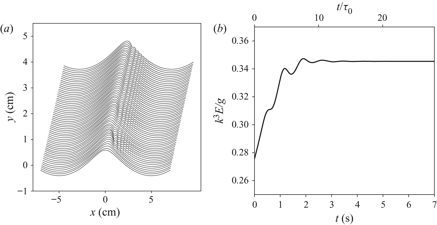
First, we consider a typical example of wave evolution towards its steady state. Figure 2(a) shows the evolution of an initially smooth and symmetric Stokes wave subjected to wind, while figure 2(b) exhibits the corresponding evolution of the wave energy (3.7). The noticeably skewed forward profile develops a train of capillary ripples on its forward slope that are frozen with respect to the primary wave, which means that the phase velocity of the ripples is exactly equal to that of the primary wave. We found that energy of the ripples, which we roughly estimate as the difference between the full energy (3.7) and the same integral with the fields  $z$ and
 $\varphi$ averaged over the small scale, ranges from 15 % of the full energy for the
 $5\ \mathrm {cm}$ waves to less than 5 % for the
 $10\ \mathrm {cm}$ and less than 1 % for the
 $25\ \mathrm {cm}$ waves.
Evolution of an initially symmetric smooth wave under the action of wind and formation of a skewed steady pattern with capillaries on the front slope. The time step between consecutive profiles is  $0.05\ \mathrm {s}$. The parameters are
 $\lambda =10\ \mathrm {cm}$,
 $u_*=20\ \mathrm {cm\ s^{-1}}$,
 $\tau _0$ is the wave period given by the linear dispersion relation. (a) Evolution of wave profile and (b) evolution of the wave full mechanical energy defined by (2.6).

It should be noted that this strictly periodic set-up does not allow consideration of waves longer than the initial wave period, thus in our simulations a potentially important aspect of the temporal evolution of wave patterns is a priori different from how wind waves evolve with fetch. In the present work we focus on the local effects occurring within one wavelength of the primary wave and do not aim at modelling a multiscale realistic wave field. The main thrust of the work is to explain why the waves of the gravity–capillary range are skewed in the way they are, but first we provide the evidence that these simulations can be trusted.
3.3. Validation
Here, we show that our results are in good agreement with other works that were using more sophisticated models with a full account of viscous effects.
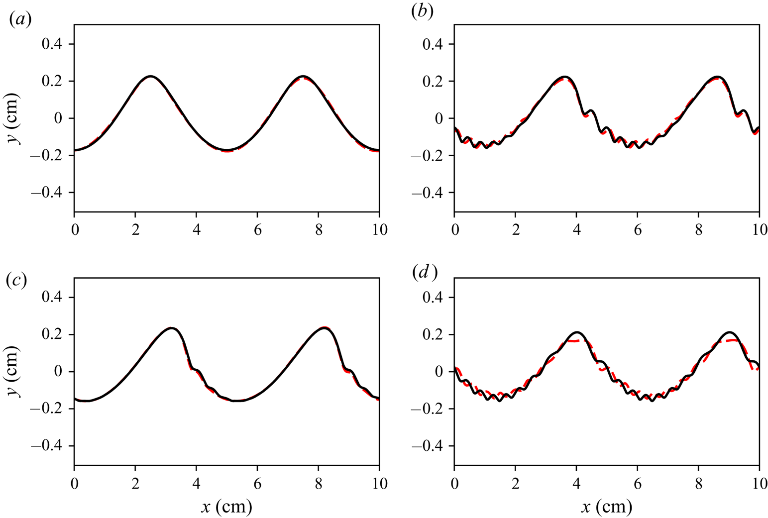
First, we reproduce a numerical experiment by Hung & Tsai (Reference Hung and Tsai2009) on ripple generation by a Stokes wave within the framework of full two-dimensional Navier–Stokes equations without wind. The initial surface profile and velocity distribution were set as a Stokes wave, that would propagate without change of form in the absence of capillarity and viscosity. Figure 3 shows profiles obtained in our simulations compared to the results of Hung & Tsai (Reference Hung and Tsai2009) with the same initial conditions. A phase velocity discrepancy of  ${\sim }5\,\%$ was observed for the primary wave, which has been adjusted when plotting the figure. We attribute the discrepancy in the wave phase velocity to the shear flow generated near the surface due to viscous effects, which our model does not capture. In Hung & Tsai (Reference Hung and Tsai2009) after the three periods of the primary wave the short ripples on the longer wave get shifted by approximately a half of their wavelength. We attribute these discrepancies to the specific way our model takes into account viscous effects. In the exact Navier–Stokes equations waves interact with a thin mean shear flow generated near the surface due to effect of viscosity (Longuet-Higgins Reference Longuet-Higgins1953; Phillips Reference Phillips1966, § 3.4); in contrast to the direct numerical simulations by Hung & Tsai (Reference Hung and Tsai2009), our model does not capture this effect. Apart from the mentioned discrepancy, there is an overall good qualitative and quantitative agreement during the first few periods for which the comparison of the two models was carried out. Note that the Hung & Tsai (Reference Hung and Tsai2009) simulations fully account for viscous dissipation, but have no wind. Hence, in their setting a steady gravity–capillary pattern with a packet of parasitic ripples on the front slope is not possible; any initially steep gravity–capillary wave leaks its energy via dissipation by parasitic capillaries, which results in a rapid decrease of its steepness and eventual loss of its parasitic capillaries.
Comparison with the Navier–Stokes simulations from Hung & Tsai (Reference Hung and Tsai2009). Evolution of an initial Stokes wave of wavelength  $\lambda =5\ \mathrm {cm}$ and steepness
 $ak=0.3$ subjected at time
 $t=0$ (in addition to gravity) to capillarity (
 $T=73\ \mathrm {cm^3\ s^{-2}}$) and viscosity (
 $\nu =0.01\ \mathrm {cm^2\ s^{-1}}$). The Navier–Stokes simulations are shown by the dashed lines, the conformal mapping results are shown by the solid lines. The phase velocity difference of
 ${\sim }5\,\%$ was adjusted when plotting this figure.
 $(a)\,\, T = 0.3,\, (b)\,\, T = 2T_{0},\, (c)\,\, T = 1T_{0}\,\, {\rm and}\,\, (d)\,\, T = 3T_{0}.$

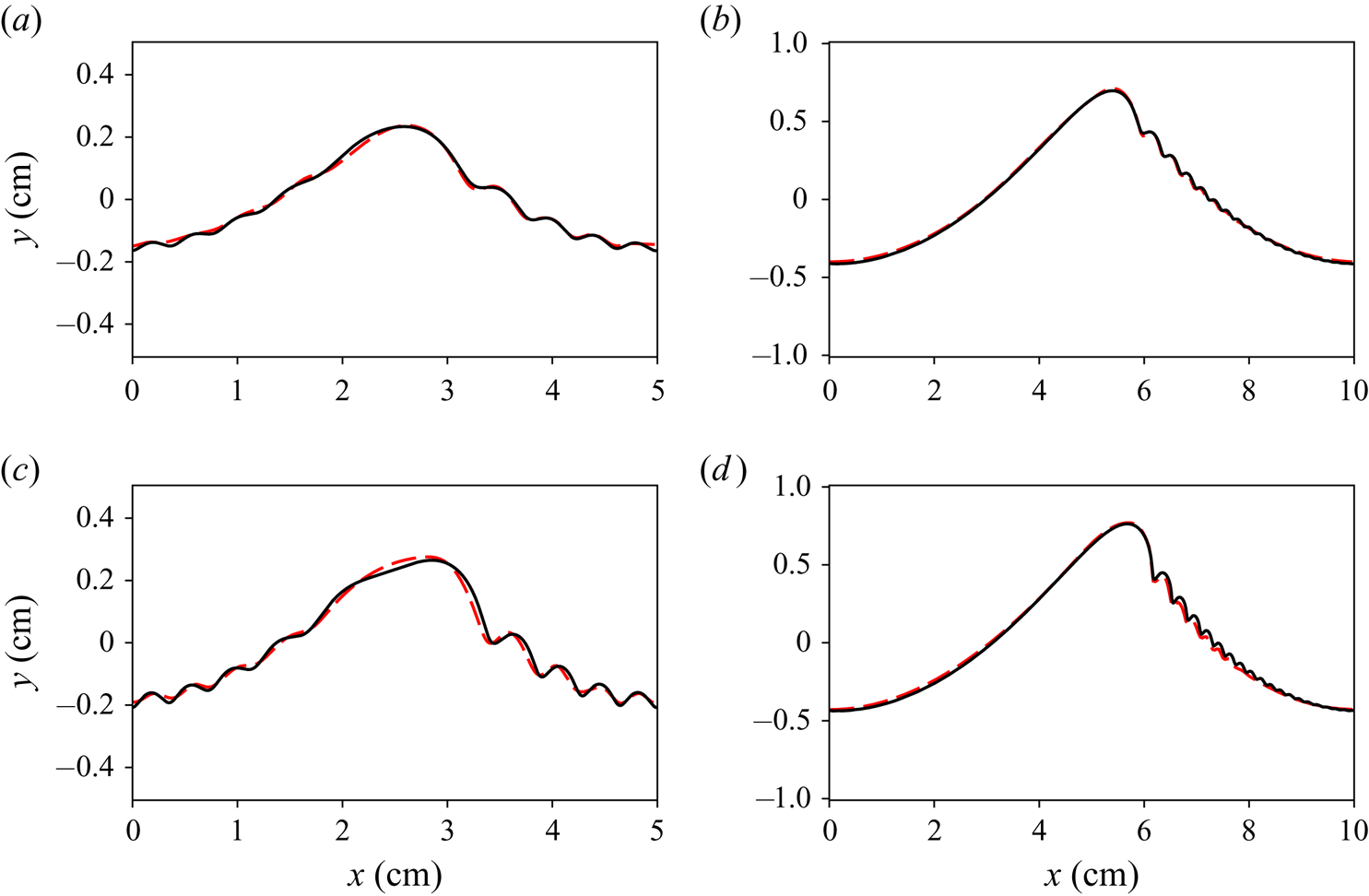
We also compare our model with a similar but more rigorous approach for steady patterns put forward by Fedorov & Melville (Reference Fedorov and Melville1998). The approach incorporates effects of the viscous boundary layer by considering a small rotational correction to the velocity field. In contrast to Fedorov and Melville we do not solve stationary equations, although we use a somewhat similar set-up; a stationary wave configuration developing from an initial disturbance of a given wavelength is considered, with energy loss due to viscosity being compensated by wind forcing. For this comparison the wind forcing (2.15) was taken as a single harmonic of pressure in phase with the wave slope. Figure 4 shows steady wave profiles obtained in such a manner (solid lines) compared with ‘Class 1’ profiles from Fedorov & Melville (Reference Fedorov and Melville1998). A reasonably close agreement is observed for a range of moderate to high amplitudes. Even higher amplitudes could not be achieved in our simulations because we avoid ripple instability and wave breaking, more details are given in the following sections.
Stationary profiles of  $\lambda =5\ \mathrm {cm}$ and
 $\lambda =10\ \mathrm {cm}$ waves (solid black lines) compared with the ‘Class 1’ profiles from Fedorov & Melville (Reference Fedorov and Melville1998) (dashed red lines). The parameters are
 $T=73\ \mathrm {cm^3\ s^{-2}}$,
 $\nu =0.01\ \mathrm {cm^2\ s^{-1}}$.
 $(a)\lambda = 5, ak = 0.250, (b)\lambda = 10, ak = 0.350, (c)\lambda = 5, ak = 0.300{\rm and}(d)\lambda = 10, ak = 0.375.$

The above favourable comparisons suggest that the approach we adopted can be used for the massive simulations needed to explore the front–back asymmetry of gravity–capillary waves, although we cannot quantify the errors caused by our assumptions; at the moment there is no viable alternative.
4. The nature of front–back asymmetry for gravity–capillary waves
4.1. How to quantify the front–back asymmetry?
We are interested in the front–back asymmetry of the mean wave profile with capillary ripples removed by filtering out high frequencies. For certainty we choose a Gaussian filter
 \begin{equation} \bar\eta(x) = \frac{1}{\sqrt{2{\rm \pi}\sigma^2}} \int\ \eta(x_1) \exp\left(-\frac{(x_1-x)^2}{2\sigma^2}\right) \, \textrm{d} x_1. \end{equation}
In this section, to illustrate the concepts we discuss, we will use as an example a numerical simulation of a  $\lambda =10\ \mathrm {cm}$ wave subjected to
 $u_*=20\ \mathrm {cm\ s^{-1}}$ wind (shown in figure 2).
The separation of scales between the primary wave and parasitic ripples is rather limited, being more narrow for smaller primary wavelengths. The size of the capillary bulb is sometimes comparable to the primary wavelength (as in the pictures of the 5 cm waves in the previous section). The distance between subsequent troughs of capillary ripples decreases gradually, filling the interval between the scale of the bulb and the smallest wavelength of capillary waves found near the trough of the primary wave. We therefore need to make sure that our definitions are robust with regard to a change of smoothing parameters.
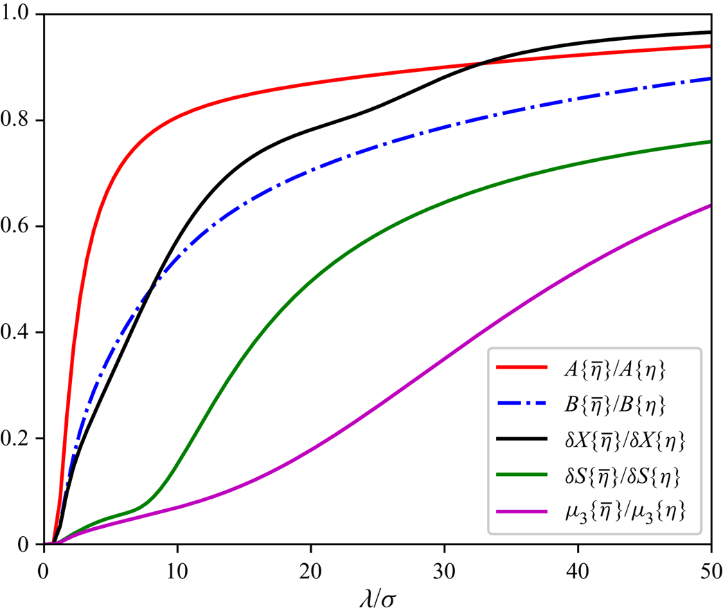
Several quantitative measures of the front–back asymmetry are being widely used. We will comment on the behaviour of each measure as we walk through their definitions. Figure 6 shows how fast each measure attains saturation as the smoothing parameter  $\sigma$ decreases (ratio
 $\lambda /\sigma$ is equivalent to the number of wave harmonics retained by the filter).
When characterising individual waves, sometimes just the displacement of the crest with regard to the surrounding troughs is considered,
 \begin{equation} \delta X = 2\frac{l_{front}-l_{rear}}{l_{front}+l_{rear}},\end{equation}
where  $l_{front}$ (
 $l_{rear}$) is the distance from the crest to the front (rear) wave trough.
One could also introduce the relative difference between the forward and backward wave slopes inclinations as
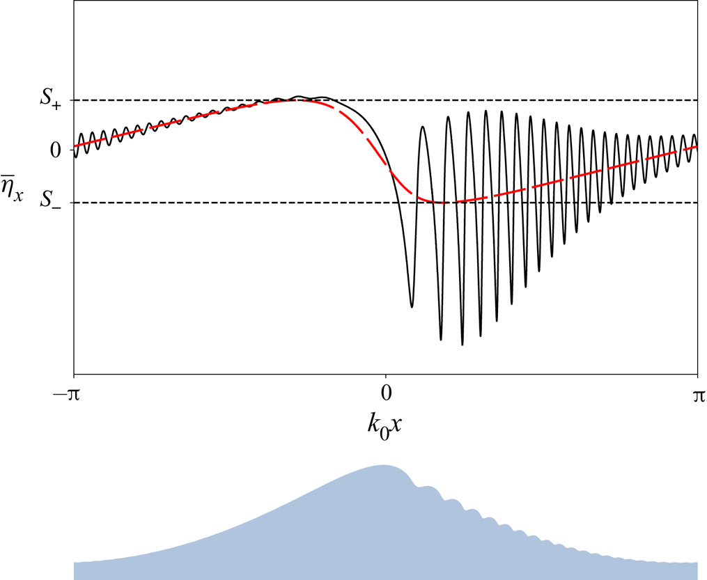
 \begin{equation} \delta S\{\bar\eta\} = \frac{|S_+|-|S_-|}{|S_+|+|S_-|}, \quad S_+=\max_x\overline{\frac{\partial\eta}{\partial x}}, \quad S_-=\min_x\overline{\frac{\partial\eta}{\partial x}}. \end{equation}
See figure 5 for illustration. Because the mean slope field is sensitive to the choice of smoothing parameters, saturation of  $\delta S\{\bar \eta \}$ with increase of
 $\lambda /\sigma$ is very slow, making it difficult to make a meaningful choice of
 $\sigma$.
Slope of the exact (black solid line) and smoothed (red dashed line) wave profile for the steady configuration with the parameters  $\lambda =10\ \mathrm {cm}$,
 $u_*=20\ \mathrm {cm\ s^{-1}}$; definitions of minimum and maximum averaged slope. At the bottom the exact elevation profile is plotted as a reference.

For a random wave field probably the best characteristic is the surface slope probability density function (PDF) used in Liu et al. (Reference Liu, Yan, Liu and Hwang1997), Munk (Reference Munk2009), Álvarez-Borrego & Martin-Atienza (Reference Álvarez-Borrego and Martin-Atienza2013), Caulliez & Guérin (Reference Caulliez and Guérin2012) and Zavadsky & Shemer (Reference Zavadsky and Shemer2017). However, in field conditions this quantity is difficult to measure and, therefore, is rarely employed. Within the PDF approach the asymmetry is characterised by the following third moment:
 \begin{equation} \mu_3 = \frac{\langle \eta_x^3\rangle} {\sqrt{\langle \eta_x^2\rangle}^3}. \end{equation}
where angle brackets mean ensemble averaging. In our particular case the wave field is steady and the ensemble averaging is replaced by the spatial average over a single wave period. Figure 6 shows that, similarly to  $\delta S$, the main contribution to
 $\mu _3$ originates from short scales. Actually, for our example profile,
 $\mu _3$ approaches saturation only at
 ${\lambda /\sigma \sim 100}$.
Saturation of various asymmetry measures with decrease of the smoothing scale  $\sigma$ for the example steady wave configuration (
 $\lambda =10\ \mathrm {cm}$,
 $u_*=20\ \mathrm {cm\ s^{-1}}$).

Bi-spectral analysis offers a simple and robust quantitative measure of asymmetry. It is defined as a third moment of the Hilbert-transformed surface elevation,  $\hat {H}[\eta ]$, is called asymmetry and denoted as
 $A$,
 \begin{equation} A\{\eta\} = \frac {\langle (\hat{H}[\eta])^3\rangle} {\sqrt{\langle \eta^2\rangle}^3}, \end{equation}
This resembles the definition for  $\mu _3$, with the derivative being replaced by the Hilbert transform. In (4.5), input from each component of the wave field is proportional to the cube of its amplitude (rather than the cube of the slope), thus it characterises properties of the principal wave, rather than the short wave components.
Quantity (4.5) can be interpreted, roughly speaking, as the normalised amplitude of the asymmetric second harmonic of the dominant wave that makes the wave profile look tilted forward or backward, depending on the phase of the second harmonic (Masuda & Kuo Reference Masuda and Kuo1981). Representing  $\eta (x)$ as a series
 \begin{equation} \eta(x) = a\cos kx +\sum_{n\geq 2}(a_n\cos nkx + b_n\sin nkx), \end{equation}
and assuming an  $a^n$ decrease of the coefficients with
 $n$, one can see that, to leading order,
 \begin{equation} A\{\eta\} = -\frac{3b_2}{\sqrt{2}a} + \frac{6(a_3b_2-a_2b_3)}{\sqrt{2}a^2} + \cdots. \end{equation}
Here, we neglect higher-order contribution in the denominator, since for strictly potential motions the second- and third-order corrections to  $\langle \eta ^2\rangle$ cancel each other (see Janssen (Reference Janssen2009) for details), and we assume the motions under consideration to be close to the potential ones. According to (4.5) the forward skewed waves, propagating in the positive direction of the axis
 $x$, have negative asymmetry. Some authors find this convention inconvenient and define asymmetry using the opposite sign (e.g. Zavadsky & Shemer Reference Zavadsky and Shemer2017).
For the example wave profile, even without applying filter (4.1), the greatest contribution to total asymmetry
 \begin{equation} A\{\eta\} = \frac{1}{\sqrt{\langle \eta^2\rangle}^3} \sum_{k_1+k_2+k_3=0} (\hat H\eta)_{k_1}(\hat H\eta)_{k_2}(\hat H\eta)_{k_3}, \end{equation}
is due to combinations of first and second harmonics of the dominant wave, so that six terms ( $|k_{1,2}|=k$,
 $|k_3|=2k$ and permutations) provide
 ${\sim }60\,\%$ of the total asymmetry. Contribution from the combinations with higher harmonics (
 $n>5$) is negligible.
One more possible approach would be to compute a norm of the asymmetric part of  $\eta$ when the origin
 $x=0$ is chosen as in (4.6)
 \begin{equation} B\{\eta\} = \frac{\lVert\frac{1}{2}(\eta(x)-\eta(-x))\rVert} {\lVert\eta(x)\rVert} = \left( \frac{\displaystyle \sum_n b_n^2}{\displaystyle a^2 + \sum_n(a_n^2+b_n^2)} \right)^{1/2}. \end{equation}
As figure 6 shows, saturation of  $B\{\bar \eta \}$ is rather slow, making it unclear what value should be attributed to the mean profile.
Since  $A\{\eta \}$ is much more robust than other measures and is often used in the analysis of wave observations (e.g. Leykin et al. Reference Leykin, Donelan, Mellen and McLaughlin1995), we choose
 $A\{\eta \}$ as the primary measure of the wave field front–back asymmetry. We will also use
 $\delta X\{\eta \}$ because it is a very common and intuitive definition of asymmetry.
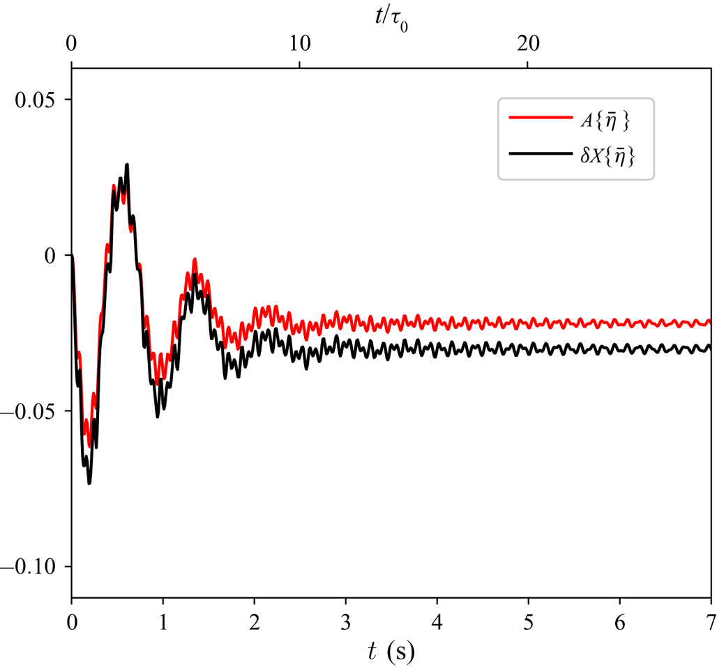
Figure 7 shows how  $\delta X\{\bar \eta \}$ and
 $A\{\bar \eta \}$ evolve with time for the same example of
 $10\ \mathrm {cm}$ wave plotted in figure 2(a). After a few large magnitude oscillations, during which asymmetry can be both positive and negative, the field settles at a moderate negative value of asymmetry.
Example of the evolution of two measures of asymmetry:  $A$ (red line) and
 $\delta X$ (black line). In the example simulation the following parameters were used:
 $\lambda =10\ \mathrm {cm}$,
 $u_*=20\ \mathrm {cm\ s^{-1}}$, smoothing parameter
 $\sigma =2\ \mathrm {cm}$.

4.2. The physical mechanism
Let us discuss the physical mechanism of how short ripples affect the shape of the principal gravity–capillary wave. The scale separation enables us to decompose dynamic variables  $\eta ,\varphi$ into a sum of mean and oscillating components,
 \begin{equation} \eta = \bar\eta+\delta\eta \quad \textrm{and}\quad \varphi = \varPhi + \delta\varphi, \end{equation}
where  $\bar \eta ,\varPhi$ describe the mean wave motion, and
 $\delta \eta ,\delta \varphi$ describe the dynamics of the ripples. We denote spatial averaging (4.1) by an overbar.
Assuming sufficient separation of scales, we average the governing equations (2.2), (2.3) to obtain the boundary conditions for the mean flow at the mean surface  $y=\bar \eta (x,t)$
 \begin{gather} \frac{\partial\bar\eta}{\partial t} + \frac{\partial\varPhi}{\partial x}\frac{\partial\bar\eta}{\partial x} - \frac{\partial\varPhi}{\partial y} + \overline{\left.\left( \frac{\partial\delta\varphi}{\partial x}\frac{\partial\delta\eta}{\partial x} \right)\right|_{y=\eta(x,t)}} = 0, \end{gather}
 \begin{gather}\frac{\partial\varPhi}{\partial t} + \frac{1}{2}|\boldsymbol{\nabla}\varPhi|^2 + \overline{g\eta + p - T\varkappa} + \frac{1}{2}\overline{|\boldsymbol{\nabla}\delta\varphi|^2|_{y=\eta(x,t)}} = 0. \end{gather}
Obviously, the equations for the mean flow are not closed. The effect of the averaged over ripples in (4.11) and (4.12) on the mean flow can be interpreted as a fictious ‘external forcing’ in the equations of motion for  $\bar \eta$ and
 $\varPhi$; an additional ‘effective mean vertical velocity’
 \begin{equation} \delta w = - \overline{\left.\left( \frac{\partial\delta\varphi}{\partial x}\frac{\partial\delta\eta}{\partial x} \right)\right|_{y=\eta(x,t)}}, \end{equation}
and an ‘effective dynamic pressure excess’ or, for brevity, an ‘effective pressure’
 \begin{equation} \delta p = \tfrac{1}{2}\overline{|\boldsymbol{\nabla}\delta\varphi|^2|_{y=\eta(x,t)}}. \end{equation}
The way we named these terms is unashamedly arbitrary and subjective, but in our view it helps in grasping their effect. Indeed, if we look closely at (4.11) and (4.12), it is easy to see that  $\delta w$ given by (4.13) acts as an extra mean vertical velocity, while the second one given by (4.14) acts as if it were an extra pressure.
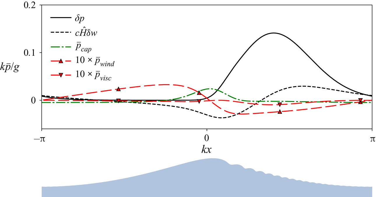
Figure 8 shows the distribution of  $\delta p$ compared to the wind
 $p_{wind}$, capillary
 $T\varkappa$ and viscous
 $p_{visc}$ pressure terms in the averaged equation (4.12) for the chosen example of stationary configuration at
 $\lambda =10\ \mathrm {cm}$,
 $u_*=20\ \mathrm {cm\ s^{-1}}$. The Hilbert transform of
 $\delta w$ is plotted alongside for the reasons explained below. The ‘effective pressure’
 $\delta p$ has a distinct maximum localised on the forward slope of the primary wave. The key point we want to stress is that for waves of gravity–capillary range effective dynamic pressure
 $\delta p$ is always much greater than all contributions to pressure due to other mechanisms.
Effective dynamic pressure  $\delta p$ compared to capillary
 $\bar p_{cap}=-T\bar \varkappa$, wind
 $\bar p_{wind}$ and viscous
 $\bar p_{visc}$ terms of the averaged equation (4.12). All terms are computed for the same example of steady configuration (
 $\lambda =10\ \mathrm {cm}$,
 $u_*=20\ \mathrm {cm\ s^{-1}}$), smoothing parameter
 $\sigma =2\ \mathrm {cm}$. The lower figure shows the elevation profile plotted as a reference.

However, establishing a substantial anomaly of the effective dynamic pressure  $\delta p$ with a distinct maximum on the forward slope of the long wave does not clarify the basic question: why are the gravity–capillary waves always skewed forward? To interpret the results of our simulations in simple terms an analytical model, however crude, is highly desirable.
In our spatially periodic set-up once a gravity–capillary wave has reached its stationary configuration, it propagates further without changing its form or phase velocity. Let us consider a situation when the main wave is moderately steep and its crest curvature is not too high, so that it does not generate intense ripples and does not require strong wind forcing to maintain the energy balance. It's dynamics is then determined primarily by gravity.
Such a steady configuration consists, apart of the principal wave, which is to leading order just  ${\sim }\cos k(x-ct)$, and a set of bound harmonics
 ${\sim }\cos nk(x-ct)$ sharpening the crest and flattening the trough, of small contributions due to wind forcing, viscosity and surface tension. Their main manifestation is a train of capillary ripples generated by the localised capillary pressure at the crest. There are localised distributions of
 $\delta p$ and
 $\delta w$ moving together with the main wave with the same phase velocity
 $c$. The principal question we have to clarify in our study of wave asymmetry is how
 $\delta p$ and
 $\delta w$ affect the amplitude and phase of the asymmetric second harmonic of the wave profile
 ${\sim }\sin 2k(x-ct)$.
The easiest way to capture analytically the main effect of our  $\delta p$ and
 $\delta w$ on the primary wave profile would be to interpret them as an external forcing and then to examine the linear response of the system to such a forcing. Strictly speaking, to find analytically the response one also has to take into account the velocity field of the primary wave, but here we neglect it and, to maximally simplify the problem, focus on the leading-order term only.
It is well known that the linear response to a harmonic pressure distribution  $p(x)=p'\sin k'x$ applied to the surface of a uniform stream is given by the simple formula (Lamb Reference Lamb1975, § 270),
 \begin{equation} \eta(x) = \frac{p'\sin k'x}{c^2k'-g-Tk^{\prime 2}}, \end{equation}
where  $c$ is the stream velocity. As explained in § 4.1, in our context, of particular interest is the second harmonic
 $k'=2k$ of the principal wave. For waves of decimetre range their phase velocity is always greater than the linear phase velocity of their second harmonic, therefore, the surface elevation (4.15) caused by an external pressure has the same sign as the applied pressure.
The surface is affected not only by a moving effective pressure  $\delta p$, but also by a moving ‘effective mean velocity’
 $\delta w$. A single harmonic of the ‘effective mean velocity’
 $\delta w(x)=W'\sin k'x$ applied in the kinetic boundary condition to a uniform stream also creates a phase-locked elevation,
 \begin{equation} \eta(x) = \frac{cW'\cos k'x}{c^2k'-g-Tk^{\prime 2}}. \end{equation}
Thus, the surface elevation (4.16) caused by an external effective mean velocity  $\delta w$ is proportional to the Hilbert transform of it. In this simplified linear consideration we can superpose contributions of
 $\delta p$ and
 $\delta w$. For a single harmonic with wavenumber
 $\check {k}$ we find
 \begin{equation} \eta = \frac{1}{c^2\check{k}-g-T\check{k}^2}(\delta p+c\hat{H}\delta w). \end{equation}
As (4.15) suggests, if  $\delta p$ is localised on the forward slope of the wave, the wave profile becomes skewed forward, which corresponds to negative asymmetry (4.5). The contribution of
 $\delta w$ slightly reduces this effect. The prediction of our very crude model agrees with the observed sign of asymmetry in our simulations and available laboratory data. Thus, we have got a simple qualitative model of the effect; a quantitative comparison with the numerical simulation results is provided in the next section.
Of course, there is no complete analogy between  $\delta p$ and true surface pressure acting upon the main wave. If it were a real pressure distribution, it would drain energy at much higher rates than wind forcing can supply.
The asymmetric wave pattern with a train of capillary ripples on the front slope is sensitive to parameters of the primary wave, which in turn are dependent on the external parameters (wind and fetch), and also on the values of surface tension and viscosity. In the next section we explore the parameter space to understand better the underlying physics and to gain insight for remote sensing.
5. Parameter space study
Here, we study how asymmetric properties of gravity–capillary waves depend on the primary wavelength  $\lambda$ and wind forcing characterised by
 $u_*$, or, given the somewhat artificial character of our wind parameterisation, by wave steepness
 $ak$. We define the amplitude
 $a$ of a given wave profile
 $\eta (x)$ as a half of its crest-to-trough height
 \begin{equation} a = \frac{h}{2}, \quad h=\max_x\bar\eta-\min_x\bar\eta. \end{equation}
For a given wave profile, the averaging parameter  $\sigma$ of the Gaussian filter (4.1) is chosen as twice the length of the first (and the longest one) ripple of the wavetrain.
Our simulations involved primary waves with wavelengths  $\lambda$ ranging from 5 to 25 cm. For a given
 $\lambda$ the lowest value of
 $u_*$ for which a non-trivial steady configuration exists is determined by balance between wind forcing and viscous decay
 $\gamma _{wind} + \gamma _{visc} = 0$. The upper bound on
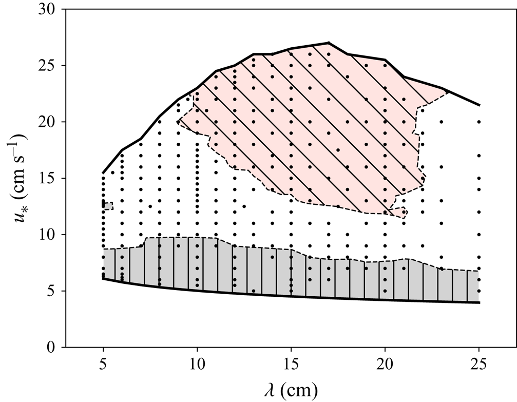
 $u_*$ that we can examine is controlled by the instability of the ripples, which causes local increase in ripple amplitude and results in self-intersection of the free surface. These limitations are shown in figure 9, which also outlines the regions of the parameter space where it takes less than 10 or more than
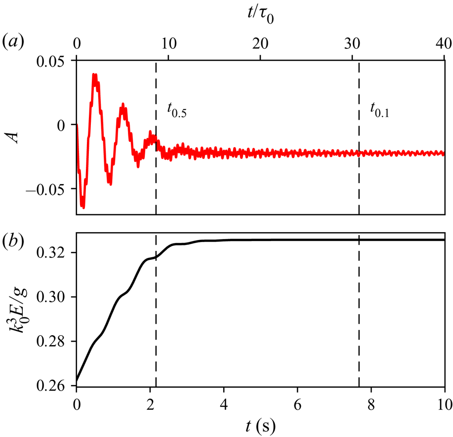
 $10^2$ linear wave periods for the oscillations around the stationary configuration to decay. To eliminate the effect of dependence on how far the initial conditions are from the resulting configuration, we define our ‘decay time’ as the duration
 $t_{osc} = t_{0.5} - t_{0.1}$ between the point
 $t_{0.5}$, where amplitude of asymmetry oscillations constitutes half of the mean asymmetry value and the point
 $t_{0.1}$ where the oscillation reduces to 0.1 of the steady value (see example in figure 10).
The parameter space of the simulations. The lower boundary of the explored domain is defined by the wind–viscosity balance condition, while the top boundary by the ripples’ instability. Marked by hatching are the regions where the stationary configuration was reached in less than 10 (slanting hatches) or in more than 100 (vertical hatches) linear wave periods.

Evolution of wave profile asymmetry  $A$ and full mechanical energy for the case of
 $\lambda =10\ \mathrm {cm}$,
 $u_*=15.0\ \mathrm {cm\ s^{-1}}$. Vertical lines indicate moments of time
 $t_{0.5}$ and
 $t_{0.1}$ when the oscillations of asymmetry reduce to
 $0.5$ or
 $0.1$ of the final asymmetry value.

As we found from simulations, the stationary configuration might depend not only on a point in the parameter space  $(\lambda , u_*)$, but also on the wave–wind history, i.e. the way the wind forcing evolved in time. In addition to our basic set-up with constant wind forcing we have tested an alternative set-up, where
 $u_*$ approached the final value gradually by small steps (
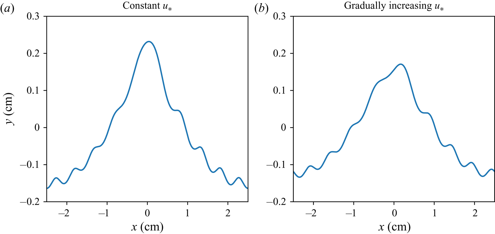
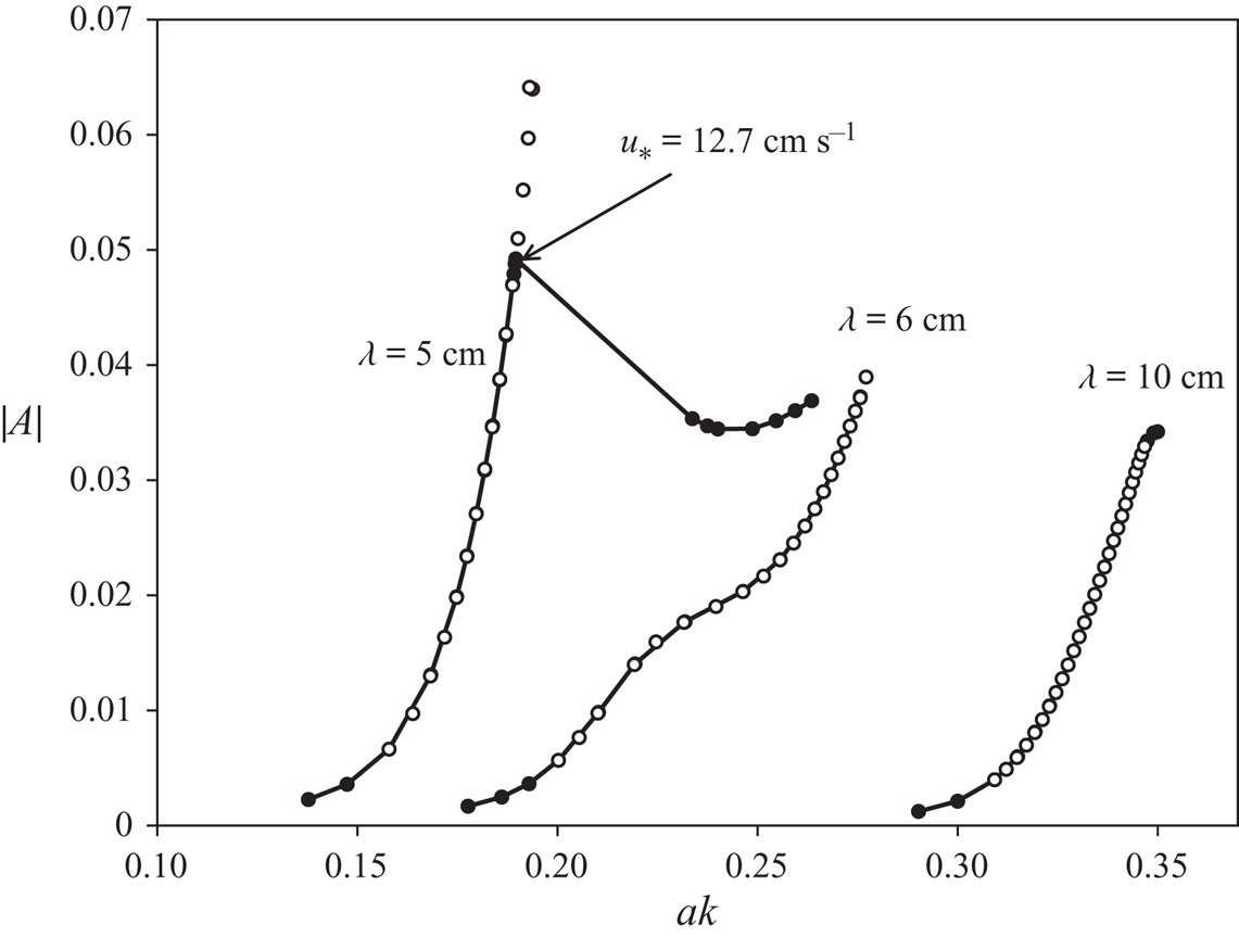
 $0.5\ \mathrm {cm\ s^{-1}}$), and sufficient time has been given after each step for the profile oscillations to decay. Figure 11 shows an example of stationary configurations for 5 cm waves obtained for the basic and the alternative set-ups; the two profiles are noticeably different and their asymmetry differs as well. A comparison between the parameters of stationary profiles obtained for the two set-ups is made in figure 12. For 5 cm waves the profiles coincide up to the point
 $u_*\approx 12.7\ \mathrm {cm\ s^{-1}}$, where the curve corresponding to the constant wind set-up diverges abruptly from the smooth dependence corresponding to the gradual increase of wind. These results indicate that the equilibrium configuration for a given point
 $(\lambda , u_*)$ is not always unique. This is an essentially novel phenomenon, which requires a dedicated investigation. Here, we just note that the domain of non-uniqueness is confined to short waves with
 $\lambda < 6\ \mathrm {cm}$. As figure 12 shows, no such bifurcation is observed for 6 cm or longer waves, and thus for most of the wavelength range discussed here the final configuration is uniquely specified by the parameters
 $(\lambda , u_*)$. We stress that the non-uniqueness of the steady state for short waves with
 $\lambda < 6\ \mathrm {cm}$ was found under the assumption of strict periodicity, at present we do not know whether this non-uniqueness is robust. Moreover, since the strictly periodic wave patterns are not observed in the real wind wave field, it is not clear what might be the manifestations of this non-uniqueness in the observations and how to design an experimental set-up and what specifically to look at to clarify this issue.
Non-uniqueness of steady short gravity–capillary waves. Stationary wave configurations obtained in the set-up with constant wind forcing (a) and in the set-up where the wind speed has been gradually increased from a small initial value (b). The parameters are  $\lambda =5\ \mathrm {cm}$,
 $u_*=13.5\ \mathrm {cm\ s^{-1}}$.

Asymmetry of the profiles obtained in the set-up with constant wind forcing (lines with black markers) and in the set-up where the wind speed has been gradually increased from a small initial value (white markers). The wavelengths are  $\lambda =5, 6, 10\ \mathrm {cm}$.

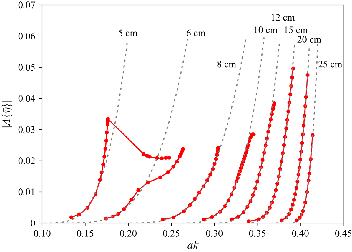
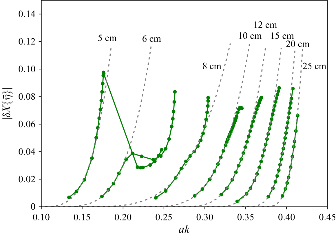
Figures 13 and 14 show how the wave profile asymmetry depends on the wave steepness for various values of the wavelength. We find it appropriate to parameterise simulated asymmetry values as
 \begin{align} |A(\lambda, ak)| = \begin{cases} 0, & \textrm{ if } ak \le a_0k \\ m^4(\lambda)\left(\dfrac{ak}{a_0(\lambda)k}-1\right)^4 & \textrm{ if }ak > a_0k, \end{cases}\end{align}
where  $m$ is a coefficient dependent on
 $\lambda$ which we find numerically. The fitting curves obtained by the least-squares method (with only lower-amplitude segments of the graph taken into account for the 5 and 6 cm waves) are shown in figures 13 and 14 by dashed lines.
Asymmetry of the wave profile as a function of steepness (solid lines with markers), and corresponding fitting curves (dashed lines) for various wavelengths.

Alternative asymmetry measure  $\delta X$ as a function of steepness. Notations as in figure 13.

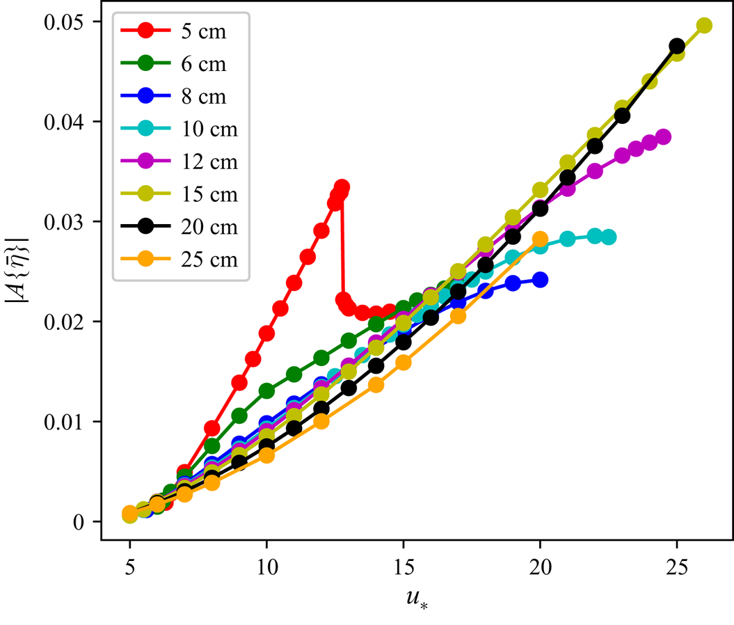
In figure 15 the asymmetry for various wavelengths is plotted against wind friction velocity  $u_*$; apart from the very short (5 cm) waves, all waves have asymmetry increasing with
 $u_*$ in a very similar way.
Asymmetry of wave profile vs  $u_*$ for various wavelengths.

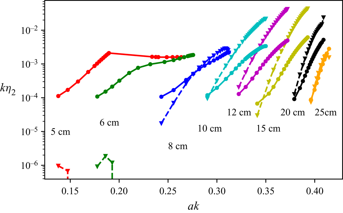
Now we can compare simulated amplitudes of the asymmetric part of second harmonic
 \begin{equation} \eta_2 = \frac{2}{\lambda}\int_0^\lambda \, \textrm{d} x \eta(x-x_0) \sin 2k(x-x_0), \end{equation}
where  $x_0$ is the position of the wave crest as computed from the phase of the first harmonic, with our rough estimate (4.17). As figure 16 shows, for the waves in the range 8–25 cm our rough estimate (4.17) captures qualitatively the dependence on steepness, although it generally overestimates the second harmonic amplitude by more than a factor of two. For small wavelengths (
 $\lambda \sim 5,\ 6\ \mathrm {cm}$) the estimate (4.17) does not work. This is probably because the distribution of
 $\delta p$ shifts more towards the wave trough, which might even result in a negative second harmonic amplitude of
 $\delta p$.
Amplitude of the second harmonic  $\eta _2$ of steady wave profiles vs steepness for various primary wavelengths: observed values (solid lines with circles) and the estimates (4.17) (dashed lines with triangles).

The results of this section suggest that configurations close to the steady ones can be expected to be commonly observed in the range of wavelengths 10–20 cm, since their formation time is very short. In contrast, the formation of steady patterns for shorter waves seems to be much less likely since their formation takes tens of wave periods. It is also worth noting that the short 5–6 cm waves also have pronounced capillary bulbs contributing to the bound second harmonic, which may be also a factor in the poor agreement between our crude analytic estimate (4.17) and the simulations.
6. Discussion and concluding remarks
In this section we will first summarise the main results and then discuss the key underpinning assumptions. Here, we will also discuss the results in the context of the available experimental data and some implications of the comparison of the model and experiments.
The main result is in revealing the principal physical mechanism of pronounced front–back asymmetry of non-breaking gravity–capillary waves. Within the framework of a nearly potential two-dimensional model it was found that in the presence of a moderate wind an arbitrary initial perturbation in the gravity–capillary range evolves into a very characteristic steady wave pattern; skewed forward with a train of parasitic capillaries on the front slope. On quantifying all the factors contributing to the asymmetry we showed that it is primarily due the Reynolds stresses caused by the train of parasitic capillaries. We called the effect of these stresses the ‘effective dynamic pressure excess’ and ‘effective mean vertical velocity’ due to parasitic capillary ripples and showed that within the framework of the adopted model it is by far the most significant factor contributing to the asymmetry observed in our simulations. Since for arbitrary initial conditions most of the waves quickly reach the steady state, we focussed upon the steady waves, which is obviously an oversimplification. To quantify the asymmetry we used two different characteristics: (i) the asymmetry based on the shift of the second harmonic of the main wave, the characteristic commonly used in a statistical description of random wave fields and (ii) the shift of the wave crests with respect to the troughs often used for the deterministic description of single waves. We showed that both these characteristics depend on the wave parameters in a similar way. Therefore, we mostly used the statistical measure of asymmetry based on the phase shift of the second harmonics of the gravity–capillary wave. To explain without simulations why the waves are skewed forward we analysed the effect a parasitic ripple envelope exerts on the original wave. At the lowest-order approximation we neglected interaction between the ripples’ envelope and the original wave itself; we estimated the perturbation in the mean wave profile as a linear response of still water to a moving distribution of dynamic pressure. Such a crude model is able to provide only a qualitative agreement with the numerical simulations (see figure 16), and this is what it is aimed at. Possibly, a quantitative agreement with the simulations could be achieved by employing a higher-order perturbation theory, however, we did not pursue this route here.
Apart from the dependence on wind discussed in the previous section and illustrated in figure 15, the characteristics of the gravity–capillary waves with parasitic capillaries also depend on the water viscosity  $\nu$ and surface tension
 $T$. Throughout the paper these parameters were assumed to be constant (
 $\nu =0.01\ \mathrm {cm^2\ s^{-1}}$ and
 $T=73\ \mathrm {cm^3\ s^{-2}}$), while in nature they vary quite noticeably. To get an idea on the sensitivity of the results to variations of
 $\nu$ and
 $T$, simulations with various
 $\nu$ and
 $T$ were performed for a fixed wavelength (
 $\lambda =10\ \mathrm {cm}$). For each combination of
 $(\nu , T)$ the wind friction velocity
 $u_*$ was adjusted in such a way that the resulting wave steepness remained the same (
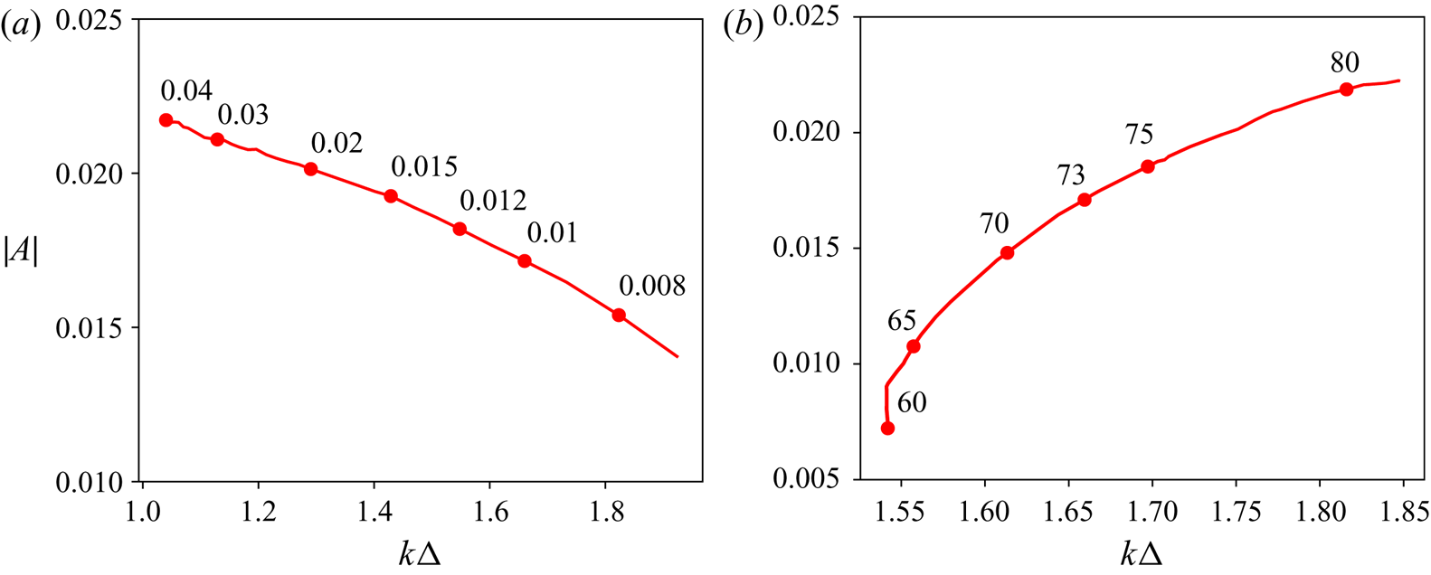
 $ak=0.33$). To interpret the obtained results it is illuminating to follow the width of the ripple package
 $\varDelta$, which we define as the full width at half-maximum of the excess pressure
 $\delta p$. Figure 17(a) shows how the asymmetry of a gravity–capillary wave depends on viscosity
 $\nu$ (at
 $T=73\ \mathrm {cm^3\ s^{-2}}$), while figure 17(b) illustrates the asymmetry dependence on surface tension
 $T$ (at
 $\nu =0.01\ \mathrm {cm^2\ s^{-1}}$).
Asymmetry and width of ripples’ wavetrain as functions of viscosity (a) and surface tension (b); the wavelength  $\lambda =10\ \mathrm {cm}$, wind forcing in each simulation is adjusted to keep the resulting wave steepness constant
 $ak=0.33$. Labels show either the coefficient of viscosity in
 $\mathrm {cm^2\ s^{-1}}$ (a) or the surface tension coefficient in
 $\mathrm {cm^3\ s^{-2}}$ (b).

As the viscous decay affects most the shortest parasitic capillaries near the end of the ripple wavetrain, a change of  $\nu$ manifests itself in both modifying the localisation of the ripple wavetrain on the primary wave slope and in suppressing the ripples. With increase of viscosity the train width
 $\varDelta$ is decreasing, that is, the excess pressure becomes more sharply localised. On the other hand, the amplitude of the ripples in the train decreases, which acts to decrease the excess effective pressure. A priori it was not clear whether the wave asymmetry decreases or increases with viscosity. One can see that, counter-intuitively, the asymmetry is growing with viscosity, that is the sharper localisation of the capillaries proved to be the dominant factor.
The picture is quite different for the case of varying surface tension. Increase in  $T$ results in the increase of capillary length scale
 $\sqrt {T/g}$ and the corresponding increase of characteristic wavelength of the ripples. That is, from the point of view of the phase synchronism between the primary wave and the ripples, the dynamics of a wave with a greater
 $T$ is similar to the dynamics of a wave with a shorter wavelength. As is shown in the previous section, the shorter waves of the same steepness tend to be more skewed forward than the longer ones.
How faithfully our simulations capture the reality is the main outstanding question that we briefly discuss here. The three key restrictive assumptions underpinning our numerical model are: (i) the strict two-dimensionality of the motion, (ii) the strict periodicity and the absence of much longer waves in the wave spectrum and (iii) the absence of wave breaking and microbreaking.
In the ocean, the gravity–capillary waves are always three-dimensional and usually are in the high-frequency tail of typical wave spectra. At present, a direct numerical simulation of a broad spectrum of three-dimensional waves resolving capillary scales fully accounting for wave nonlinearity is far beyond our reach. However, we could try to get a rough idea of the importance of these factors. The employed assumption of strict periodicity is certainly restrictive. In particular, it totally excludes the effects due to wave groups which are known to strongly affect the instantaneous asymmetry; waves first lean forward and then backward as they sweep through the envelope (Slunyaev & Shrira Reference Slunyaev and Shrira2013; Banner et al. Reference Banner, Barthelemy, Fedele, Allis, Benetazzo, Dias and Peirson2014). What the contribution is of these substantial oscillations of asymmetry to the ensemble averaged quantities is not known; the issue has never been studied. In the ocean gravity–capillary waves nearly always are also modulated by much longer gravity waves, which can profoundly alter our conclusions on their front–back asymmetry. To get a rough idea on how the gravity–capillary wave asymmetry is affected by the presence of much longer waves, we have conducted a simulation of a decimetre range Stokes wavetrain modulated by a much longer wave of realistic steepness (10 m long wave with the steepness  $ak=0.09$). The initial distributions of gravity–capillary wave amplitude and wavenumber were prescribed in such a way that the corresponding wave action flux, as well as the local frequency, were constant along the long wave profile. That is, at each point the gravity–capillary wave amplitude and wavelength are equal to those of a wavetrain that has travelled to that point all the way from, say, the longer wave trough, being modulated by the long wave orbital velocity (but not subjected to the action of wind or viscous decay). The chosen set-up allows us to postpone the gravity–capillary wave focusing and subsequent breaking.
If the definition (4.5) were applied directly to quantify asymmetry of a gravity–capillary wave riding on a long wave, it would yield very small values everywhere except for a neighbourhood of points where the elevation of the long wave vanishes, since the denominator in (4.5) incorporates the root mean square value of total surface elevation  $\eta$. It is therefore more informative to subtract the long wave elevation profile before computing (4.5). A sample simulation illustrating the spatio-temporal evolution of the short wave asymmetry over ten seconds can be viewed in supplementary movie available at https://doi.org/10.1017/jfm.2020.696.
The simulation shown in supplementary movie illustrates the complexity of the asymmetry dynamics in the presence of a much longer wave. In particular, note the high instantaneous values of  $|A|$ occurring in the process.
Longer time simulations were not attempted. Our very limited preliminary study of the effect of much longer waves on the asymmetry suggests that the effect of the long waves on asymmetry is of order one and has to be taken into account. However, the account of long waves results in a complicated behaviour of wave patterns with strongly varying asymmetry. The key feature which greatly simplified our analysis, the emergence of steady gravity–capillary wave patterns, disappears in the presence of long waves. The likely but unverified explanation is that long waves sweeping through the gravity–capillary wavetrain destroy the tight link between the first and second harmonics of the gravity–capillary wave, as a result the short wave crests start to oscillate. This also resembles the behaviour observed in wave groups, where the wave crests lean forward and backward as they propagate through the envelope (Slunyaev & Shrira Reference Slunyaev and Shrira2013; Banner et al. Reference Banner, Barthelemy, Fedele, Allis, Benetazzo, Dias and Peirson2014). The problem certainly needs a dedicated study. Even in the absence of long waves the assumption of periodicity is quite restrictive.
Three-dimensional effects we have not accounted for can be essential since the three-dimensional waves can be steeper (without breaking) and, therefore, more asymmetric. At present, the contribution of wave field three-dimensionality is unknown. It is known, however, that in the absence of long waves gravity–capillary wind waves of decimetre range form a distinctive rhombic pattern made of two oblique dominant waves at angles  $\pm \theta$ to the wind direction, with the typical value of
 $\theta$ being
 $\approx 30^\circ$ (Caulliez & Collard Reference Caulliez and Collard1999). The synchronism condition for generation of ripples by an oblique wave selects shorter oblique waves with the same downwind component of the wave vector. It is certainly interesting and challenging to extend our analysis to three-dimensional waves, but our a priori guess is that the differences will be quantitative, not qualitative.
The unaccounted effects of wave breaking and microbreaking are expected to be crucially important for asymmetry for situations beyond the range of applicability of the presented model. Below we briefly discuss the available laboratory data and the new insight they provide.
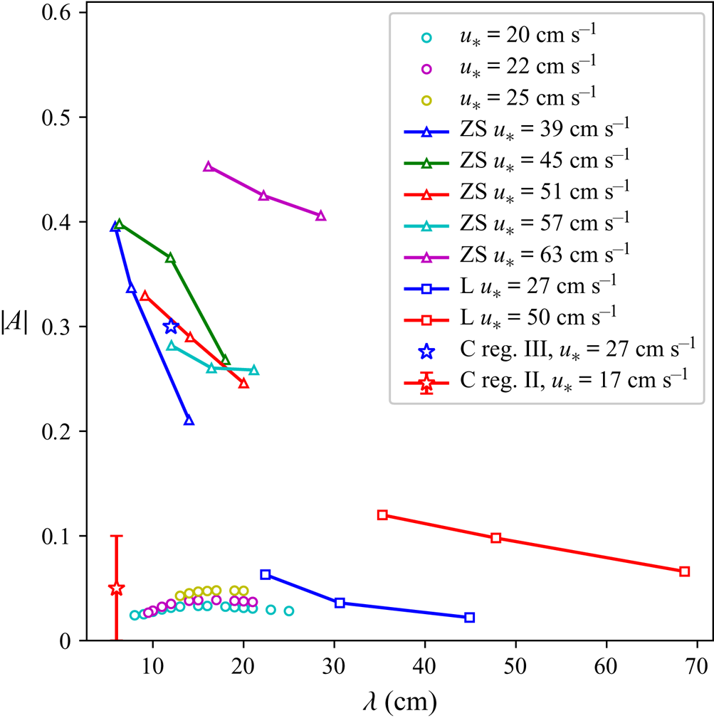
An idea about the relevance of our results can be obtained by their, at a glance, comparison with the available laboratory measurements of the front–back asymmetry of gravity–capillary waves carried out in Leykin et al. (Reference Leykin, Donelan, Mellen and McLaughlin1995), Caulliez (Reference Caulliez2013) and Zavadsky & Shemer (Reference Zavadsky and Shemer2017). The available experimental data, as well as our simulation results, are brought together in figure 18 showing the dependence of wave profile asymmetry  $A$ on the primary wavelength for various moderate winds. We stress that most of the experimental points were obtained for winds substantially stronger than those in the model. Both Leykin et al. (Reference Leykin, Donelan, Mellen and McLaughlin1995) and Zavadsky & Shemer (Reference Zavadsky and Shemer2017) employ the definition of asymmetry (4.5) based on the imaginary part of the elevation bi-spectra (recall that the asymmetry definition in Zavadsky & Shemer (Reference Zavadsky and Shemer2017) differs in sign, so that the waves skewed forward have positive asymmetry). The measurements of Leykin et al. (Reference Leykin, Donelan, Mellen and McLaughlin1995) were carried out on fetches from 8 to 20.9 m, and of Zavadsky & Shemer (Reference Zavadsky and Shemer2017) from 1.2 to 3.4 m.
Comparison of the simulation results (circles) with experimental measurements by Leykin et al. (Reference Leykin, Donelan, Mellen and McLaughlin1995) (lines with squares, only  $u_*<80\ \mathrm {cm\ s^{-1}}$), Caulliez (Reference Caulliez2013) (stars) and Zavadsky & Shemer (Reference Zavadsky and Shemer2017) (lines with triangles).

At the lowest values of wind forcing  $u_*=27\ \mathrm {cm\ s^{-1}}$ examined by Leykin et al. (Reference Leykin, Donelan, Mellen and McLaughlin1995) (see their table 1) the absolute values of asymmetry for 22.4 cm waves are up to 2 times greater than the characteristic asymmetry for 20–25 cm waves in our simulations, while the observed mean wave steepness
 $ak \approx 0.17$ is substantially lower than the threshold of ripple generation for the same wavelength in our simulations (
 $a_0 k \sim 0.35$). Two points should be noted here: First, since our model does not account for the effect of a drift current which substantially affects the dispersion relation for these scales, a direct comparison of the model and the Leykin et al. (Reference Leykin, Donelan, Mellen and McLaughlin1995) measurements is very problematic without drift current measurements. Second, the fact that the mean steepness is below the threshold of ripple generation does not imply that all wave crests are subcritical, this just means that the characteristic capillary trains we focus upon are intermittent, they occur only on the some of the crests.
Zavadsky & Shemer (Reference Zavadsky and Shemer2017) do not provide the peak frequencies or wavelengths observed in their experiments. The wavelengths in figure 18 correspond to peak frequencies of elevation spectra in their figure 1 with the Doppler shift correction made according to their equation (2). The reported asymmetry values  $|A| \sim 0.3$ are almost an order of magnitude greater than those obtained in our numerical simulations (
 $|A| \sim 0.05$), and the wave steepness is relatively low throughout their experiments (
 $ak \sim 0.2$).
Although it may be not entirely correct to equate parameter  $u_*$ in our wind forcing parameterisations (2.15) with the true wind friction velocity, the large discrepancy in the range of
 $u_*$ in the laboratory and simulations is striking; in the experiments
 $u_*$ was significantly higher (
 $u_* > 35\ \mathrm {cm\ s^{-1}}$ in Zavadsky & Shemer (Reference Zavadsky and Shemer2017) and
 $u_* > 27\ \mathrm {cm\ s^{-1}}$ in Leykin et al. Reference Leykin, Donelan, Mellen and McLaughlin1995) than the threshold below which a steady pattern of ripples could be formed in our simulations.
In Caulliez (Reference Caulliez2013) the records of surface elevations of gravity–capillary waves were analysed from the viewpoint of dominant dissipation mechanisms. In particular, two wave regimes which were distinguished which are of special interest in our context: (i) ‘regime II’ was identified as a special regime where neither breaking nor microbreaking occurs, (ii) the regime with microbreaking, but without breaking was labelled as ‘regime III’. The values of asymmetry were not provided, but several realisations of the elevation records enabled us to calculate asymmetry  $A$ as an average over available sample profiles for these regimes. The results of these calculations are indicated by stars: red star for the regime II and blue star for the regime III. To give an idea of the scatter of the experimental values we also indicated the confidence interval for the regime II. A comparison of our model predictions with the asymmetries found for the ‘regime II’ and ‘regime III’ profiles from Caulliez (Reference Caulliez2013) (figures 4 and 5 there) leads to the key insight into the nature of the discrepancies between the model and experiments. In the non-breaking nor microbreaking ‘regime II’ (observed at fetch
 $6\ \mathrm {m}$, wind speed
 $5\ \mathrm {m\ s^{-1}}$) the dominant waves have wavelengths
 $\lambda \sim 6\ \mathrm {cm}$, their dissipation being primarily due to parasitic ripple generation. For the five profiles given in the paper the maximum absolute value of asymmetry is
 $\max |A\{\bar \eta \}| \approx 0.1$ (we set the averaging parameter
 $\sigma =1\ \mathrm {cm}$ here) and the arithmetic mean of the five asymmetry values is
 $-0.05$. It is this arithmetic mean which is indicated in figure 18 by stars (for this regime, and for regime III), the scatter of the values of
 $A$ in the individual realisations for the regime II is also shown by red vertical line. Note that in all experiments the wave field is random and the waves are never steady. Our simulations of asymmetry for steady non-breaking 6 cm waves yield
 $A \approx -0.02$, although absolute values of
 $A$ could be up to
 $0.1$ during the transition (the specific values depend on the initial amplitude of the Stokes wave). Given the large scatter of the experimental values of
 $A$ we can conclude that in this regime the predictions based on our simulations agree reasonably well with the experimental data. Although the model predictions fall onto the centre of the experimental scatter, this might also be due to coincidence.
In the ‘regime III’, according to the classification by Caulliez (Reference Caulliez2013), (observed at fetch  $6\ \mathrm {m}$, wind speed
 $7\ \mathrm {m\ s^{-1}}$) the characteristic wavelength of the dominant waves is
 $\lambda \sim 12\ \mathrm {cm}$, and these waves are dissipating due to both microbreaking and parasitic ripples, with the former being the dominant energy sink. In the observations the maximal absolute value of asymmetry does not exceed
 $\max |A\{\bar \eta \}| \approx 0.6$, while the arithmetic mean of asymmetry is
 $-0.3$. In our simulations the steady profiles of non-breaking
 $12\ \mathrm {cm}$ waves have asymmetry up to
 $A\approx -0.04$, while during the transition the absolute values are only a bit larger, up to
 $0.05$. A notable difference here is that in the experimental data wave profiles exhibit much higher asymmetry while still having rather moderate steepness (
 $ak\approx 0.3$), close to the ripple generation threshold
 $a_0k$ in the simulations. We stress that the model is not supposed to describe this regime.
Thereby, there is a qualitative and, at least, an order of magnitude agreement for the ‘regime II’ of Caulliez (Reference Caulliez2013), i.e. for the particular regime where both breaking and microbreaking are totally absent. However, for the regimes with even a moderate amount of microbreaking (‘regime III’), there are substantial discrepancies between the model and observations. In the model, as figure 15 shows, asymmetry grows almost linearly with increase of  $u_*$ despite some signs of saturation for short waves (
 $\lambda < 10\ \mathrm {cm}$). This suggests that even higher values of asymmetry might be possible with further increase of
 $u_*$, although in the corresponding regime, characterised by ripple instability, their breaking and entrapment of air bubbles – the microbreaking, currently cannot be properly modelled.
Therefore, it is reasonable to assume that the main factor contributing to high asymmetry values in the gravity–capillary waves observed in regime III of Caulliez (Reference Caulliez2013), Leykin et al. (Reference Leykin, Donelan, Mellen and McLaughlin1995) and Zavadsky & Shemer (Reference Zavadsky and Shemer2017) which is not accounted for by the model is the microbreaking. For longer waves it might be the occurrence of breaking waves. It is a formidable challenge to incorporate the microbreaking and breaking into the model. Note that, to attain quantitative agreement, the surface shear current that affects differently the ripples and gravity–capillary waves, and the horizontal inhomogeneity of this current in the laboratory tank, causing kinematic transformation of the peak waves, should be also accounted for in the modelling.
Overall, there remains a substantial gap to overcome to develop a useful model of the asymmetry for remote sensing and for air–sea interaction applications. This discussion enabled us to identify the key mechanisms (microbreaking and breaking) which are the first we need to master the modelling.
The results discussed so far were confined to surfactant-free water. The presence of surfactants, i.e. surface films of biological or mineral origin that are common in nature, is expected to change the picture qualitatively, the issue needs a dedicated investigation.
On the conceptual level the results could be applied not only to gravity–capillary waves, but to all types of waves where a similar synchronism of waves of different scales takes place. The class of wave systems where such synchronism is allowed is immensely rich, we mention just a few examples of waves of different nature having this property: flexural–gravity waves in water covered by an ice sheet modelled as an elastic plate, internal gravity waves, edge waves, Rossby waves (e.g. Mysak & LeBlond Reference Mysak and LeBlond1978). It is not difficult to imagine situations where the energy is pumped into the longer waves, which would lead to the generation of much shorter waves in synchronism with the longer one. Again, it is natural to expect the shorter waves to be subjected to some form of dissipation and to be linearly or nonlinearly decaying. Although it is not clear how relevant the issue of front–back asymmetry might be for such waves, here, we just note that the qualitative understanding obtained by examining gravity capillary waves enables us to predict a priori whether the longer waves in the synchronism will be skewed forward or backward. Indeed, if there is such a synchronism and the longer wave is of sufficient amplitude to generate an analogue of parasitic capillaries on the crest, the sign of asymmetry of possible two-scale pattern is determined by the location of the train of shorter waves similar to parasitic capillaries. In this reasoning it is implicitly assumed that the train of shorter waves decays rapidly enough and thus the area of shorter waves is confined to a fraction of the longer wave wavelength. The location of such a patch of short waves is determined only by a single property of the dispersion relation, namely, whether the group velocities of shorter waves are faster or slower than the phase speed of longer ones. In the examples we mentioned, the breakdown is as follows: in cases of gravity capillary waves and flexural–gravity waves under ice the shorter waves have higher group velocity and, therefore, their train will be located on the front slope and the longer wave will be skewed forward; in contrast, the edge waves, internal gravity waves and Rossby waves will have their localised trains of short waves on their back slope and, correspondingly, will be skewed backward.
Acknowledgements
The work would not have been possible without the support through the EU grant FP7 612610, which is gratefully acknowledged. The work was also partly supported by UK NERC grant NE/S011420/1. A.D. acknowledges support from RFBR grant No. 18-35-00658.
Declaration of interests
The authors report no conflict of interest.
Supplementary movie
Supplementary movies are available at https://doi.org/10.1017/jfm.2020.696.