



1 Introduction
The discovery of unstable invariant solutions of the Navier–Stokes equations, such as stationary/travelling waves and periodic orbits, has led to significant advancement in the understanding of transition and turbulence at low Reynolds numbers. Many of these solutions have been found in wall-bounded shear flows, such as plane Couette, pressure-driven channel and pipe flows, and boundary layer flows (e.g. Nagata Reference Nagata1990; Kawahara & Kida Reference Kawahara and Kida2001; Waleffe Reference Waleffe2001; Faisst & Eckhardt Reference Faisst and Eckhardt2003; Wedin & Kerswell Reference Wedin and Kerswell2004; Hall & Sherwin Reference Hall and Sherwin2010; Park & Graham Reference Park and Graham2016, and many others). These invariant solutions form a state-space skeleton (Gibson, Halcrow & Cvitanovic Reference Gibson, Halcrow and Cvitanovic2008; Willis, Cvitanovic & Avila Reference Willis, Cvitanovic and Avila2013, Reference Willis, Cvitanovic and Avila2016), and their understanding from a dynamical systems viewpoint has played the key role in illuminating the nature of bypass transition and low-Reynolds-number turbulence. It has also recently been shown that computation of these invariant solutions with a suitable modelling of surrounding small-scale turbulence may also be relevant to the description of large-scale coherent structures emerging at much higher Reynolds number (Rawat et al. Reference Rawat, Cossu, Hwang and Rincon2015; Hwang, Willis & Cossu Reference Hwang, Willis and Cossu2016).
Recently, several researchers have discovered a self-similar form of some invariant solutions in the core region of plane Couette flow with respect to the given spanwise length scale (Blackburn, Hall & Sherwin Reference Blackburn, Hall and Sherwin2013; Deguchi Reference Deguchi2015; Eckhardt & Zammert Reference Eckhardt and Zammert2016). In particular, Deguchi (Reference Deguchi2015) showed that the smallest possible invariant solutions emerge at the Kolmogorov microscale using an asymptotic theory. These findings are very intriguing, as the self-similar nature of the invariant solutions down to the Kolmogorov scale is seemingly reminiscent of the eddy structures expected in the Richardson–Kolmogorov energy cascade (Kolmogorov Reference Kolmogorov1941, Reference Kolmogorov1991). However, it should be pointed out that the energy cascade is also a well-established concept in turbulent flows even without any mean shear (isotropic turbulence) (see e.g. Vassilicos Reference Vassilicos2015), whereas the invariant solutions, at least of the type mentioned here, would not exist in the absence of mean shear.
Indeed, the question of whether or not there exists a link between the self-similar invariant solutions and the eddies in the energy cascade is very puzzling. On the one hand, the invariant solutions have often been understood to underpin a sustaining mechanism of energy-carrying eddies (i.e. coherent structures) via the so-called self-sustaining process (SSP) (Hamilton, Kim & Waleffe Reference Hamilton, Kim and Waleffe1995; Waleffe Reference Waleffe1997) and/or vortex–wave interaction (VWI) (Hall & Smith Reference Hall and Smith1991; Hall & Sherwin Reference Hall and Sherwin2010). This process is essentially a two-way interaction between wavy streaks and streamwise vortices, and, in particular, the amplification process of streaks by streamwise vortices (i.e. ‘lift-up’ effect) involves production of turbulent kinetic energy – the production term in the standard turbulence budget equation has the same mathematical origin with the off-diagonal term in the Orr–Sommerfeld and Squire equations that represents the lift-up effect (Hwang Reference Hwang2016). On the other hand, when considering the cascade, the Kolmogorov microscale is essentially derived by considering the scale at which the rate of ‘energy transfer’ from large scale (equivalent to the rate of turbulence dissipation) is expected to be balanced with viscous dissipation (Kolmogorov Reference Kolmogorov1941, Reference Kolmogorov1991). Therefore, eddies at the Kolmogorov scale in the energy cascade should be mainly driven by the energy transferred from large scales. However, for invariant solutions the energy production and dissipation are in perfect balance on the scale of the structure. Also, in general, not all eddies at the Kolmogorov microscale are the outcome of the energy cascade in a high-Reynolds-number turbulent flow. An important example of this is near-wall turbulence in and below the buffer layer. The integral length scale in this region is the viscous inner length scale
 $\unicode[STIX]{x1D6FF}_{\unicode[STIX]{x1D708}}=\unicode[STIX]{x1D708}/u_{\unicode[STIX]{x1D70F}}$
(
 $\unicode[STIX]{x1D708}$
is the kinematic viscosity and
 $u_{\unicode[STIX]{x1D70F}}$
is the friction velocity), and this is identical to the corresponding Kolmogorov length scale.
Motivated by this puzzling issue, the goal of the present study is to report our observation that there exists a turbulence production mechanism at the Kolmogorov microscale in the bulk region of turbulent Couette flow, where the invariant solutions at the Kolmogorov microscale have been found (e.g. Deguchi Reference Deguchi2015). This mechanism is found to essentially originate from the uniform local mean shear in the flow, and, interestingly, we shall see that the related eddy turn-over dynamics is remarkably similar to the SSP/VWI. A numerical experiment that removes all the structures except those in the core of the channel is also performed, and we demonstrate that the energy-producing structures in the bulk region sustain themselves, suggesting that the invariant solutions at the Kolmogorov microscale are likely to underpin the dynamics of these structures. Finally, it should be mentioned that, given the definition of the Kolmogorov microscale, dissipation of the energy produced by these self-sustaining structures must take place at the same scale, thereby consistent with the nature of the invariant solutions that exhibits perfect balance between production and dissipation on the scale of the structure.
2 Background
2.1 Mean-momentum balance
We consider a turbulent flow bounded by two infinitely long and wide parallel walls. Here,
 $x$
,
 $y$
and
 $z$
denote the streamwise, wall-normal and spanwise direction, and the corresponding velocities are
 $u$
,
 $v$
and
 $w$
, respectively. The two walls are located at
 $y=-h$
and
 $y=h$
, and they slide in opposite directions with speeds
 $u|_{y=-h}=-U_{w}$
and
 $u|_{y=h}=U_{w}$
. A fundamental feature of the turbulent Couette flow is the mean-momentum balance, obtained by taking average of the streamwise momentum equation in time and two homogeneous directions:
 $$\begin{eqnarray}\unicode[STIX]{x1D708}\frac{\text{d}U}{\text{d}y}-\overline{u^{\prime }v^{\prime }}=\frac{\unicode[STIX]{x1D70F}_{0}}{\unicode[STIX]{x1D70C}},\end{eqnarray}$$
where
 $U$
is the mean velocity,
 $\overline{u^{\prime }v^{\prime }}$
the Reynolds shear stress (the overbar denotes the average in time and two homogeneous directions),
 $\unicode[STIX]{x1D70F}_{0}$
the applied shear stress, and
 $\unicode[STIX]{x1D70C}$
the density of the fluid. Here, we note that the validity of (2.1) is not limited only to the Couette flow – any parallel flow driven by a shear stress uniform in
 $y$
should satisfy this equation. Therefore, equation (2.1) must be viewed as the generic mean-momentum equation for flows driven by a locally uniform shear stress.
Equation (2.1) provides some important physical insight into the velocity and length scales relevant to the present investigation. Since (2.1) is valid at every wall-normal location, the local shear flow can be viewed as the outcome of the applied local shear stress
 $\unicode[STIX]{x1D70F}_{0}$
. This implies that the local velocity scale would be given from the local shear stress, such that
 $u_{\unicode[STIX]{x1D70F}}=\sqrt{\unicode[STIX]{x1D70F}_{0}/\unicode[STIX]{x1D70C}}$
. We note that if the wall-normal location is chosen to be at the wall (i.e.
 $y=\pm h$
),
 $u_{\unicode[STIX]{x1D70F}}$
becomes identical to the friction velocity in the near-wall region. However, in the present case,
 $u_{\unicode[STIX]{x1D70F}}$
also becomes the local velocity scale at every wall-normal location, as it originates from the constant shear stress
 $\unicode[STIX]{x1D70F}_{0}$
in the wall-normal direction. It is also important to note that (2.1) itself does not contain any description of the ‘integral’ length scale associated with the largest admissible eddies, and the scale of the largest eddies is here determined by the size of the computational domain. If the computational domain were sufficiently large horizontally, the relevant length scale of the largest admissible eddies would be given by the height of the channel. However, if the computational domain were artificially narrowed in the spanwise direction down to
 $O(\unicode[STIX]{x1D6FF}_{\unicode[STIX]{x1D708}})$
, as in a typical minimal channel simulation (Jiménez & Moin Reference Jiménez and Moin1991; Hwang Reference Hwang2013), the size of the largest admissible eddies would be restricted to
 $O(\unicode[STIX]{x1D6FF}_{\unicode[STIX]{x1D708}})$
. In this case, the rate of turbulence dissipation would be given by
 ${\mathcal{E}}\sim u_{\unicode[STIX]{x1D70F}}^{3}/\unicode[STIX]{x1D6FF}_{\unicode[STIX]{x1D708}}$
, and the corresponding Kolmogorov length scale becomes identical to the viscous inner length scale: i.e.
 $\unicode[STIX]{x1D702}=\unicode[STIX]{x1D6FF}_{\unicode[STIX]{x1D708}}$
. Normalising (2.1) with
 $u_{\unicode[STIX]{x1D70F}}$
and
 $\unicode[STIX]{x1D702}$
then leads to
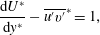 $$\begin{eqnarray}\frac{\text{d}U^{\ast }}{\text{d}y^{\ast }}-\overline{u^{\prime }v^{\prime }}^{\ast }=1,\end{eqnarray}$$
where the superscript
 $^{\ast }$
indicates the resulting dimensionless variables. Here, we note that the use of the superscript
 $^{\ast }$
, instead of the commonly used
 $^{+}$
for normalisation by the viscous inner units, is to highlight that the associated velocity and length scales are relevant to all wall-normal locations, including the outer and centreline region, where the use of the viscous inner scales would not usually make sense.
In (2.2), it is evident that the values of
 $\text{d}U^{\ast }/\text{d}y^{\ast }$
and
 $\overline{u^{\prime }v^{\prime }}^{\ast }$
from a DNS with a sufficiently large horizontal computational domain would be strongly dependent upon the wall-normal location, as a range of different length scales would come into play at each of the wall-normal locations – this can be easily checked by inspecting the available DNS database (see e.g. Pirozzoli, Bernardini & Orlandi Reference Pirozzoli, Bernardini and Orlandi2014). However, if the size of the eddies were artificially restricted to the given Kolmogorov length scale, the velocity and length scales of the eddies at play would be uniquely given by
 $u_{\unicode[STIX]{x1D70F}}$
and
 $\unicode[STIX]{x1D702}$
. Therefore,
 $\text{d}U^{\ast }/\text{d}y^{\ast }$
and
 $\overline{u^{\prime }v^{\prime }}^{\ast }$
are expected to be constant along the wall-normal direction, except the near-wall region where the no-slip boundary condition would break the homogeneity of (2.2). One such solution, but trivial, is given by
 $\text{d}U^{\ast }/\text{d}y^{\ast }=1$
and
 $\overline{u^{\prime }v^{\prime }}^{\ast }=0$
. However, the presence of non-zero mean shear in the flow system considered here also suggests that there may exist other non-trivial solutions of (2.2) that involve non-zero Reynolds shear stress and the resulting turbulence production. The objective of the present study is essentially to address this point.
2.2 Minimal Couette flow up to
 $Re_{\unicode[STIX]{x1D70F}}\simeq 800$

To seek the production mechanism at the Kolmogorov microscale, a set of minimal-span direct numerical simulations (
 $L_{z}^{\ast }\simeq 100{-}140$
) are performed. This approach, originally designed to investigate the self-sustaining nature of near-wall turbulence (e.g. Jiménez & Moin Reference Jiménez and Moin1991; Hamilton et al.
Reference Hamilton, Kim and Waleffe1995; Hwang Reference Hwang2013), has recently been extended to study low-dimensional dynamics of the structures in the logarithmic and outer regions (Flores & Jiménez Reference Flores and Jiménez2010; Hwang Reference Hwang2015; de Giovanetti, Hwang & Choi Reference de Giovanetti, Hwang and Choi2016; Hwang & Bengana Reference Hwang and Bengana2016) as well as to assess the effect of wall roughness with economical computational cost (Chung et al.
Reference Chung, Chan, MacDonald, Hutchins and Ooi2015; MacDonald et al.
Reference MacDonald, Chung, Hutchins, Chan, Ooi and Garcia-Mayoral2017). The numerical solver used in this study is diablo, the detailed numerical method of which is well documented in Bewley (Reference Bewley2014). In this solver, the streamwise and spanwise directions are discretised using Fourier series with a 2/3 dealiasing rule, whereas the wall-normal direction is discretised using a second-order central difference. The time integration is performed semi-implicitly based on the fractional-step method (Kim & Moin Reference Kim and Moin1985). All the terms with wall-normal derivatives are implicitly advanced using a second-order Crank–Nicolson method, while the rest of the terms are explicitly integrated using a third-order low-storage Runge–Kutta method. This solver has been verified through our previous studies (e.g. Hwang Reference Hwang2013).
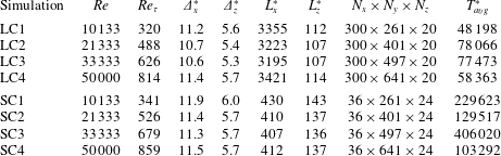
Table 1 summarises the simulation parameters in the present study. The simulations are performed up to
 $Re=50\,000$
(
 $Re\equiv U_{w}h/\unicode[STIX]{x1D708}$
), and the corresponding friction Reynolds number is found to be
 $Re_{\unicode[STIX]{x1D70F}}\simeq 800$
(
 $Re_{\unicode[STIX]{x1D70F}}\equiv u_{\unicode[STIX]{x1D70F}}h/\unicode[STIX]{x1D708}$
). We note that this value of friction Reynolds number is much smaller than that expected from a simulation with a sufficiently large computational domain, as will be discussed in detail in § 4.2. Both long and short streamwise computational domains are considered: the former with
 $L_{x}^{\ast }\simeq 3000$
is used to identify the full statistical features, while the latter with
 $L_{x}^{\ast }\simeq 400$
is used to inspect the low-dimensional dynamics of the motions in the minimal spanwise domain. As was extensively discussed in Hwang (Reference Hwang2013), numerical simulations with such a minimal spanwise domain contain a non-physical two-dimensional motion resolved by zero spanwise wavenumber (i.e. spanwise-independent cross-flow motion). This motion is essentially driven by the quasi two-dimensional nature of the present computational domain, and has been found to be dependent upon the size of the streamwise domain. This motion is therefore eliminated by adopting the filtering approach in Hwang (Reference Hwang2013). Finally, it should be mentioned that the spanwise domain and the filtering of the two-dimensional motions here do not affect the mean-momentum balance in (2.2), as the equation for zero streamwise and spanwise wavenumbers in our numerical solver (i.e. the spatial mean equation) is not directly modified by them (see also figure 2
c). Therefore, the time average of this equation with the spanwise-minimal domain and the removal of the spanwise-independent cross-flow motion still yields the one identical to (2.2).
Simulation parameters in the present study (after dealiasing), and
 $T_{avg}^{\ast }$
is the time interval for average. Here,
 $\unicode[STIX]{x1D6E5}_{x}^{\ast }$
and
 $\unicode[STIX]{x1D6E5}_{z}^{\ast }$
are grid spacings in the
 $x$
- and
 $z$
-directions, and
 $N_{x}$
,
 $N_{y}$
and
 $N_{z}$
are the number of grid points in the
 $x$
-,
 $y$
- and
 $z$
-directions, respectively. In the name of simulations, LC indicates ‘long channel’ and SC ‘short channel’ in the streamwise direction.
3 Results and discussion
3.1 Turbulence statistics
An instantaneous flow field of LC4 simulation. Here, the blue iso-surfaces indicate
 ${u^{\prime }}^{\ast }=-2$
, while the red ones are
 ${v^{\prime }}^{\ast }=1.5$
.

We first consider simulations with a long streamwise computational domain (i.e. LC simulations in table 1). Figure 1 is a visualisation of an instantaneous streamwise and wall-normal velocity field from the simulation performed at the highest Reynolds number (i.e. LC4). The flow field is occupied by small-scale eddies, the spanwise size of which just fits in the given spanwise computational domain. The motions associated with the streamwise velocity fluctuation (blue iso-surface in figure 1) tend to be elongated in the streamwise direction, but they are not very long. This feature becomes more evident if their streamwise extent is compared with that of the eddies in the near-wall region: the near-wall streamwise velocity fluctuation appears to be much longer than that in the bulk region of the flow. On the other hand, the streamwise extent of the wall-normal velocity fluctuations in the bulk region is slightly shorter than that for the streamwise velocity, and it does not seem to be greatly changed in the near-wall region (red iso-surface in figure 1).
Turbulence statistics for mean-momentum balance and production: (a)
 $U^{\ast }(y^{\ast })$
; (b)
 $-\overline{u^{\prime }v^{\prime }}^{\ast }$
; (c)
 $(\text{d}U^{\ast }/\text{d}y^{\ast })-\overline{u^{\prime }v^{\prime }}^{\ast }$
; (d)
 $-\overline{u^{\prime }v^{\prime }}^{\ast }\,(\text{d}U^{\ast }/\text{d}y^{\ast })$
. Here,
 $\cdots \cdots$
, LC1; – ⋅ – ⋅ –, LC2; - - - -, LC3; ——, LC4.
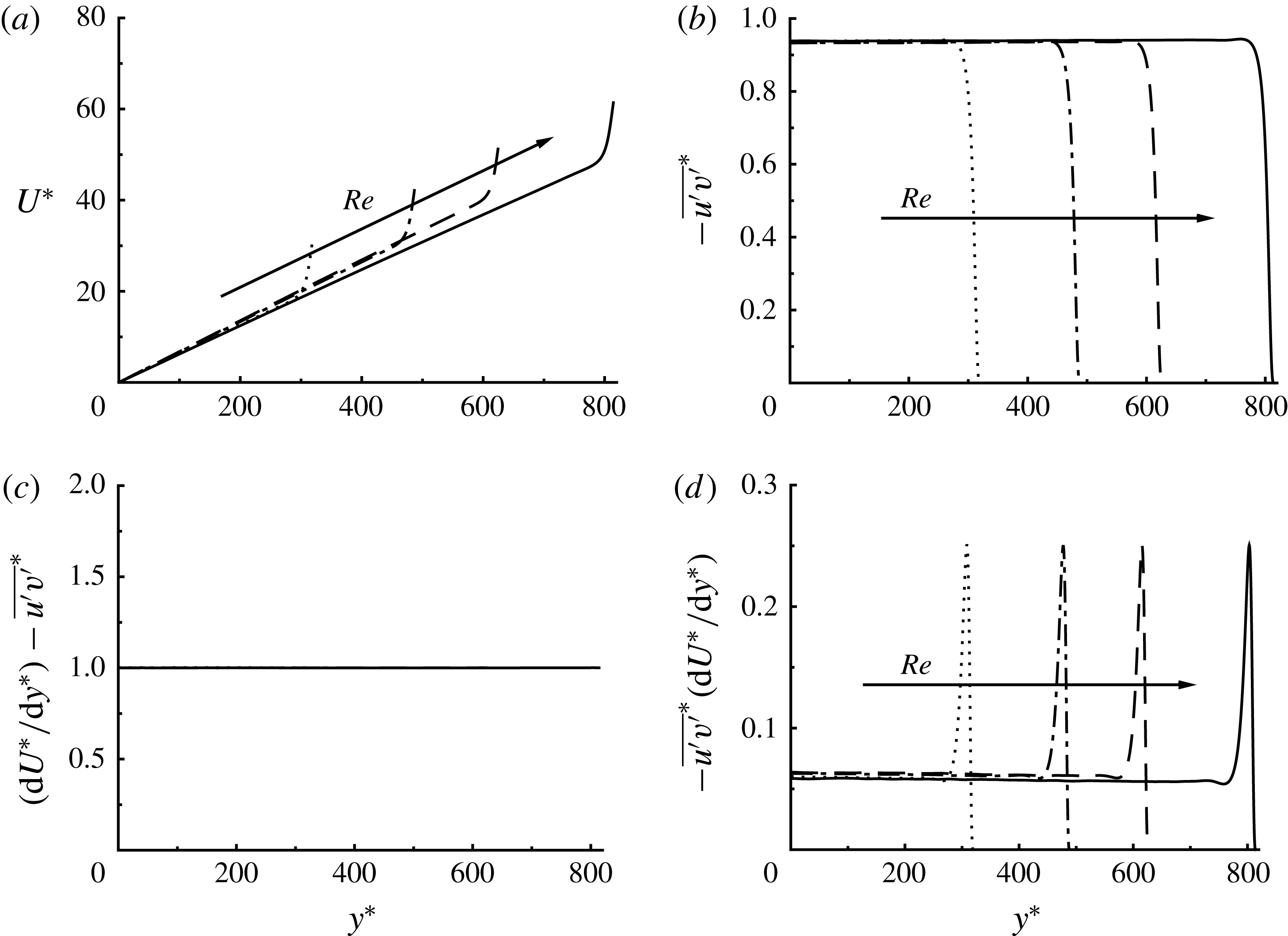
Figure 2 shows turbulence statistics involved in the construction of the mean-momentum balance and turbulence production. Here, the wall-normal coordinate in figure 2 is given by
 $y^{\ast }=y/\unicode[STIX]{x1D702}$
, so that
 $y^{\ast }=0$
corresponds to the centreline of the channel. This unconventional choice for the wall-normal coordinate is specifically to distinguish the Kolmogorov length scale
 $\unicode[STIX]{x1D702}$
from the viscous inner length scale
 $\unicode[STIX]{x1D6FF}_{\unicode[STIX]{x1D708}}$
. In the present study, we also show the statistics only for the upper half of the channel, as they are symmetric about
 $y^{\ast }=0$
. The mean velocity profile and the Reynolds shear stress for all the considered Reynolds numbers show impressively clear scaling with
 $u_{\unicode[STIX]{x1D70F}}$
and
 $\unicode[STIX]{x1D702}$
at all the wall-normal locations, except in the near-wall region where
 $y^{\ast }$
is largest (figure 2
a,b). In the bulk region, both the mean shear rate and the Reynolds shear stress are almost constant, being
 $\text{d}U^{\ast }/\text{d}y^{\ast }\simeq 0.07$
and
 $-\overline{u^{\prime }v^{\prime }}^{\ast }\simeq 0.93$
. They also exactly satisfy the mean-momentum balance in (2.2) throughout all wall-normal locations (figure 2
c), demonstrating that the spanwise-minimal domain and the filtering of the two-dimensional motions do not affect the mean-momentum balance (2.2). Finally, the constant values of the mean shear rate and the Reynolds shear stress at the Kolmogorov scale also imply a non-zero constant value of turbulence production given by
 $-\overline{u^{\prime }v^{\prime }}^{\ast }\,(\text{d}U^{\ast }/\text{d}y^{\ast })\simeq 0.065$
(figure 2
d). This evidently indicates that the turbulence production mechanism can indeed be active at the Kolmogorov microscale in the bulk region of the flow.
Turbulent velocity fluctuations: (a)
 $u_{rms}^{\ast }(y^{\ast })$
; (b)
 $v_{rms}^{\ast }(y^{\ast })$
; (c)
 $w_{rms}^{\ast }(y^{\ast })$
. Here,
 $\cdots \cdots$
, LC1; – ⋅ – ⋅ –, LC2; - - - -, LC3; ——, LC4.

The velocity fluctuations are shown in figure 3. As expected, all the turbulent velocity fluctuations exhibit very good scaling with
 $u_{\unicode[STIX]{x1D70F}}$
and
 $\unicode[STIX]{x1D702}$
over all wall-normal locations, except the near-wall region. In the bulk region, the velocity fluctuations are found to be
 $u_{rms}^{\ast }\simeq 1.7$
,
 $v_{rms}^{\ast }\simeq 0.93$
and
 $w_{rms}^{\ast }\simeq 1.3$
. The different values of the velocity fluctuations suggest that the eddies populating the bulk are anisotropic, as one might expect given the presence of mean shear. In the near-wall region, the anisotropic nature of the velocity fluctuations becomes very strong: in particular, the magnitude of the near-wall streamwise velocity fluctuation is much larger than that in the bulk region; the other components vary only a little in the near-wall region before the drop in the viscous sub-layer. The near-wall velocity fluctuations are also found to scale very well in the wall-normal coordinate normalised by the viscous inner length scale (i.e.
 $y^{+}=(y+h)/\unicode[STIX]{x1D6FF}_{v}$
), consistent with the case of pressure-driven minimal turbulent channel (Hwang Reference Hwang2013). However, this issue does not exactly fall within the scope of the present study, and the related discussion is given in the Appendix.
One-dimensional premultiplied (a,c,e,g) spanwise and (b,d,f,h) streamwise wavenumber spectra of (a,b) streamwise velocity, (c,d) wall-normal velocity, (e,f) spanwise velocity and (g,h) Reynolds stress. Here: shaded, LC1; solid, LC4. In (a,b), the contour levels are 0.125, 0.25 and 0.375 times of each of the maximum, while in (c–h), they are 0.25, 0.5 and 0.75 times of each of the maximum.

One-dimensional spectra also exhibit essentially uniform statistics in the bulk region. Figure 4 shows the spanwise and streamwise wavenumber spectra of streamwise, wall-normal, spanwise velocities and Reynolds shear stress from the lowest and the highest Reynolds numbers (LC1 and LC4). All the spectra in figure 4 exhibit remarkably good scaling with
 $u_{\unicode[STIX]{x1D70F}}$
and
 $\unicode[STIX]{x1D702}$
, while being constant at all wall-normal locations except the near-wall region. The peaks in the spanwise wavenumber spectra of all the variables (figure 4
a,c,e,g) appear at the largest spanwise wavelength, indicating that the spanwise size of the motions at all the wall-normal locations in the flow field is restricted by the narrow spanwise computational domain (note that the motions uniform in the spanwise direction are eliminated in the simulations, as discussed in § 2.2). The streamwise wavenumber spectra are also shown to indicate the streamwise length scale of the structures in the bulk region. The streamwise extent of the streamwise velocity structure is characterised by
 $\unicode[STIX]{x1D706}_{x}^{\ast }\simeq 300$
(figure 4
b), whereas that of the wall-normal and spanwise velocity structures is
 $\unicode[STIX]{x1D706}_{x}^{\ast }\simeq 200$
(figure 4
d,f). The streamwise length scale of the Reynolds shear stress is rather similar to that of the streamwise velocity spectra, revealing the peak at
 $\unicode[STIX]{x1D706}_{x}^{\ast }\simeq 300$
(figure 4
h). The spectra in the near-wall region are much more anisotropic than those in the bulk region, and their peaks generally appear at larger streamwise wavelengths. The overall features of the spectra in the near-wall region are almost identical to those observed in the spanwise-minimal unit of pressure-driven channel flow (Hwang Reference Hwang2013), as discussed in the Appendix (see also figure 14).
The wall-normal correlation functions with the reference point at
 $y_{ref}=0$
: (a)
 $R_{uu}(r^{\ast };0)$
; (b)
 $R_{vv}(r^{\ast };0)$
; (c)
 $R_{ww}(r^{\ast };0)$
. Here,
 $\cdots \cdots$
, LC1; – ⋅ – ⋅ –, LC2; - - - -, LC3; ——, LC4.
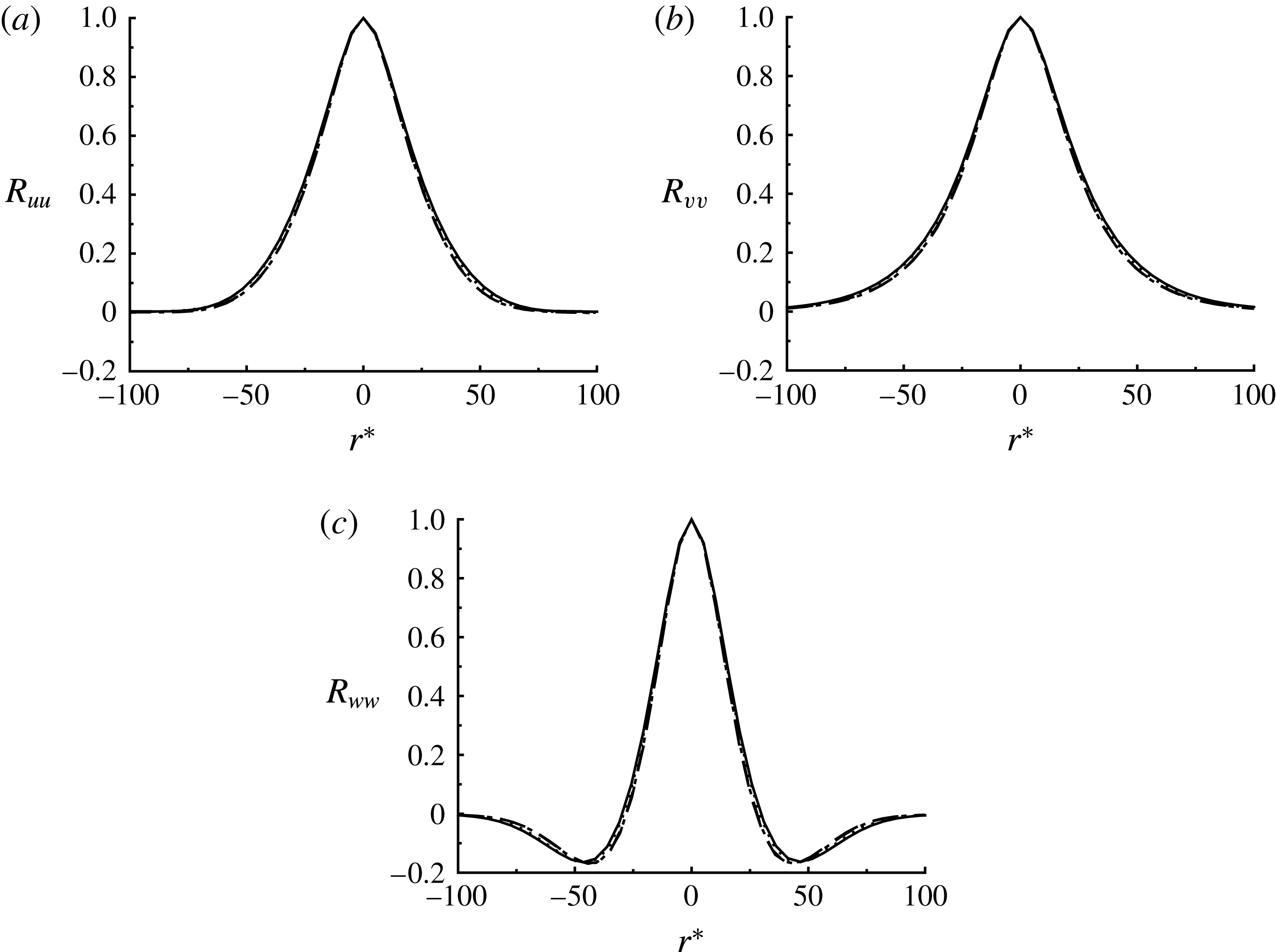
Figure 1 clearly shows that the wall-normal size of the eddies in the bulk region is not very large, which follows from the fact that all the turbulence statistics are constant in the wall-normal direction (figures 2–4). Therefore, to characterise the wall-normal size of the eddies, a two-point correlation function in the wall-normal direction is introduced. For example, the correlation function for the streamwise velocity is given by
 $$\begin{eqnarray}R_{uu}(r;y_{ref})=\frac{\overline{u^{\prime }(y_{ref}+r)u^{\prime }(y_{ref})}}{\overline{u^{\prime }(y_{ref})u^{\prime }(y_{ref})}},\end{eqnarray}$$
where
 $y_{ref}$
is the reference point. Similarly, the correlation functions for the wall-normal and spanwise velocities are computed, and denoted by
 $R_{vv}(r;y_{ref})$
and
 $R_{ww}(r;y_{ref})$
, respectively.
The computed correlation functions with
 $y_{ref}=0$
(i.e. the centre of the channel) are shown in figure 5 at all the Reynolds numbers considered. All the computed correlation functions for each velocity component are almost identical when they are scaled with the Kolmogorov length scale
 $\unicode[STIX]{x1D702}$
. Their tails are found to reach zero roughly at
 $r^{\ast }\simeq \pm 50\sim \pm 100$
, indicating that the wall-normal size of the eddies would be
 $l^{\ast }\simeq 50\sim 100$
. This also implies that the constant turbulence statistics in the bulk region of the flow along the wall-normal direction (figures 2–4) are due to the homogeneous distribution of the statistically and dynamically identical eddies at the Kolmogorov scale at all wall-normal locations except the near-wall. In this respect, it should be mentioned that any solutions of the Navier–Stokes equation with uniform shear flow would be invariant under a wall-normal translation, as long as the solutions are not affected by boundary conditions that would break the invariance (e.g. no-slip condition). It is evident that the eddies in the bulk region of the present numerical simulations belong to this case, and the only expected difference between the eddies at different wall-normal locations should therefore be their mean streamwise advection velocity.
3.2 Self-sustained structures at the Kolmogorov scale
Temporal evolution of flow field in the core region (
 $0\leqslant y^{\ast }\leqslant 50$
) from the SC2 simulation: (a) time trace of
 $E_{u}^{\ast }$
(solid) and
 $E_{v}^{\ast }$
(dashed); (b) magnification of (a) for
 $t^{\ast }\in [1476,1658]$
; (c–f) the corresponding flow visualisation. In (c–f), the red and blue iso-surfaces indicate
 ${u^{\prime }}^{\ast }=-1.2$
and
 ${v^{\prime }}^{\ast }=0.8$
, respectively.
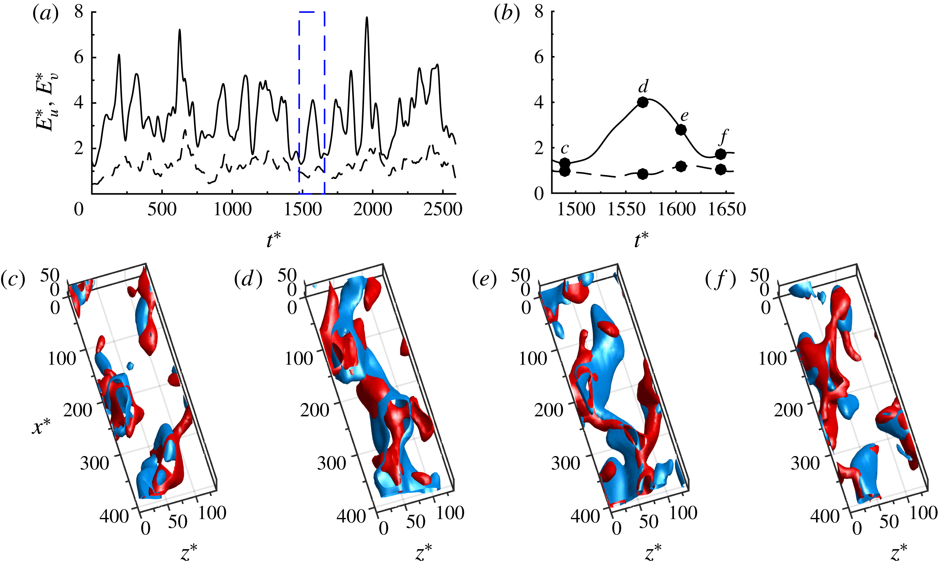
Now, to study low-dimensional dynamics of the motions in the bulk region, we consider a much shorter streamwise computational box size (SC cases in table 1). Particular emphasis of this section is given to find any links between the dynamics of the eddies in the bulk region and the SSP/VWI. Instantaneous flow fields around
 $y^{\ast }=0$
are first inspected while tracking the turbulent kinetic energy of each velocity component obtained by averaging over a small domain around the centreline: i.e.
 $$\begin{eqnarray}E_{u}^{\ast }=\frac{1}{V^{\ast }}\int _{\unicode[STIX]{x1D6FA}^{\ast }}{u^{\ast }}^{2}\,\text{d}V,\quad E_{v}^{\ast }=\frac{1}{V^{\ast }}\int _{\unicode[STIX]{x1D6FA}^{\ast }}{v^{\ast }}^{2}\,\text{d}V,\quad E_{w}^{\ast }=\frac{1}{V^{\ast }}\int _{\unicode[STIX]{x1D6FA}^{\ast }}{w^{\ast }}^{2}\,\text{d}V,\end{eqnarray}$$
where
 $\unicode[STIX]{x1D6FA}^{\ast }=[0,L_{x}^{\ast }]\times [0,L_{y}^{\ast }]\times [0,L_{z}^{\ast }]$
with
 $l_{y}^{\ast }=50$
and
 $V^{\ast }$
is the volume of
 $\unicode[STIX]{x1D6FA}^{\ast }$
. Here, we note that the size of
 $\unicode[STIX]{x1D6FA}^{\ast }$
is chosen to be just enough for a single eddy at the Kolmogorov length scale (see also the wall-normal autocorrelation in figure 5).
Temporal auto correlation: (a)
 $C_{uu}(\unicode[STIX]{x1D70F}^{\ast })$
; (b)
 $C_{vv}(\unicode[STIX]{x1D70F}^{\ast })$
; and (c)
 $C_{ww}(\unicode[STIX]{x1D70F}^{\ast })$
. Here,
 $\cdots \cdots$
, SC1; – ⋅ – ⋅ –, SC2; - - - -, SC3; ——, SC4. Note that all the correlation functions are almost identical when normalised by the Kolmogorov scales.
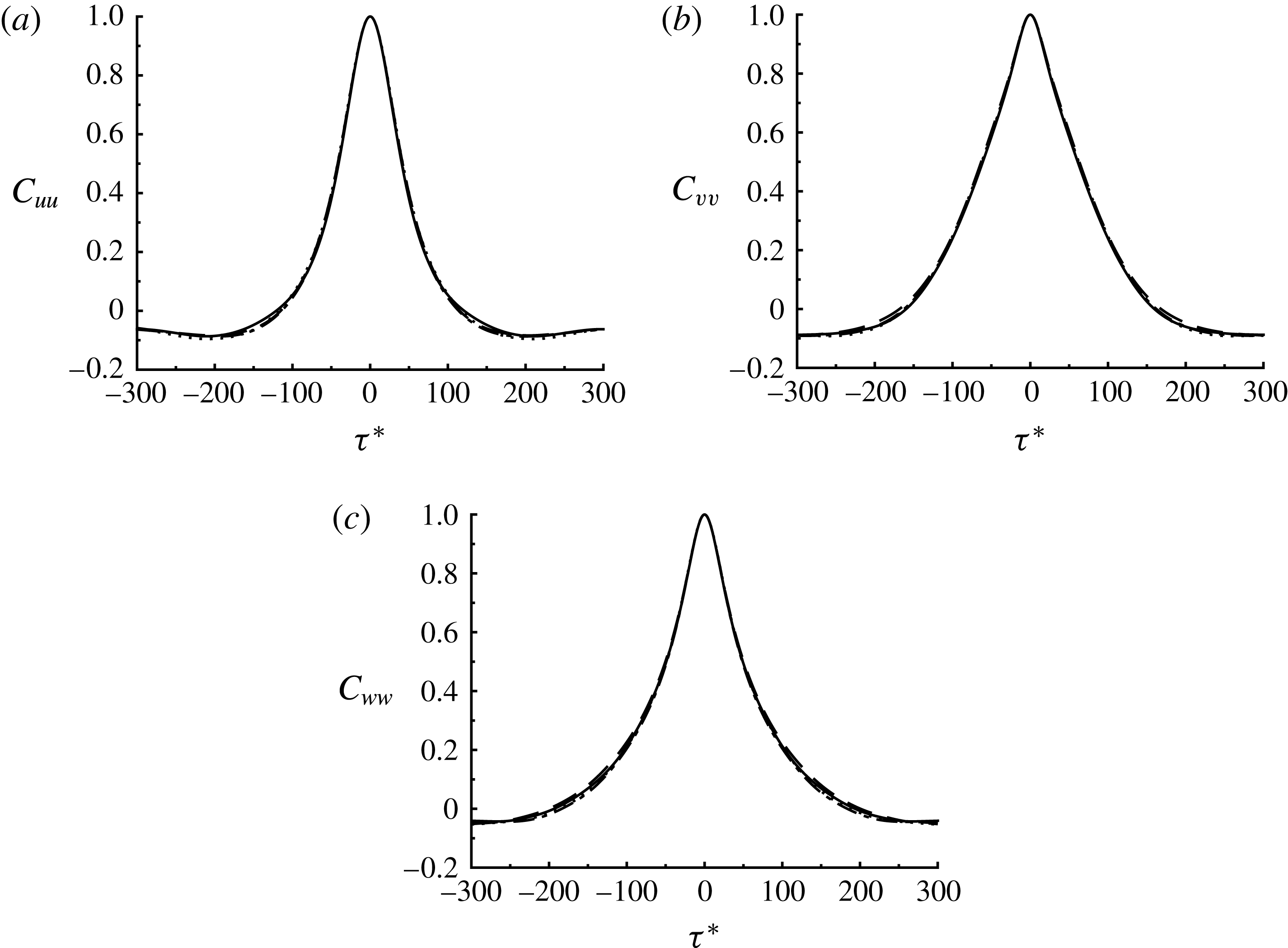
Figure 6 shows the temporal evolution of
 $E_{u}^{\ast }$
and
 $E_{v}^{\ast }$
and the corresponding flow visualisation in the region
 $\unicode[STIX]{x1D6FA}^{\ast }$
. Since
 $E_{v}^{\ast }$
and
 $E_{w}^{\ast }$
have been found to show strong correlation (see figure 11
d),
 $E_{w}^{\ast }$
is not shown here for brevity. Both
 $E_{u}^{\ast }$
and
 $E_{v}^{\ast }$
show temporal oscillations with a time scale of
 $T^{\ast }\simeq 200\sim 300$
(figure 6
a), and occur with some phase difference. Although the flow fields are fairly chaotic in general and the structures are also found to often move up and down across the wall-normal boundary of
 $\unicode[STIX]{x1D6FA}^{\ast }$
, a careful observation leads us to conclude that the overall behaviour of the flow fields is quite similar to the SSP/VWI observed in Hamilton et al. (Reference Hamilton, Kim and Waleffe1995). The strong wall-normal velocity structures (figure 6
c) are transformed into a highly amplified and elongated streamwise velocity structure, reminiscent of a ‘streak’ (figure 6
d). The amplified streamwise velocity structure meanders along the streamwise direction (figure 6
e), and eventually breaks down with regeneration of the wall-normal velocity structures (figure 6
f). This process occurs in a cyclic manner, detailed later with respect to figure 11.
The eddy turn-over dynamics observed in figure 6 is also found to scale very well with the Kolmogorov microscale. This is shown by computing correlation functions with the variables defined in (3.2):
 $$\begin{eqnarray}C_{ij}(\unicode[STIX]{x1D70F})=\frac{\langle E_{i}^{\ast }(t+\unicode[STIX]{x1D70F})E_{j}^{\ast }(t)\rangle }{\sqrt{\langle {E_{i}^{\ast }}^{2}(t)\rangle }\sqrt{\langle {E_{j}^{\ast }}^{2}(t)\rangle }},\end{eqnarray}$$
where
 $i,j=u,v,w$
and
 $\langle \cdot \rangle$
indicates average in time. Figure 7 shows the autocorrelations computed for all the Reynolds numbers. They are indeed almost indistinguishable when scaled by
 $u_{\unicode[STIX]{x1D70F}}^{\ast }$
and
 $\unicode[STIX]{x1D702}$
. The autocorrelation functions of all the variables reach zero at
 $t^{\ast }\simeq \pm 100\sim \pm 150$
, suggesting that the time scale of the eddy turn-over dynamics in figure 6 would be
 $T^{\ast }\simeq 200\sim 300$
. Interestingly, this time scale is almost identical to that of the self-sustaining process in near-wall turbulence (e.g. Jiménez et al.
Reference Jiménez, Kawahara, Simens, Nagata and Shiba2005) (see also § 4.1 for further discussion).
The visual inspection of a series of flow fields suggests that the eddies at the Kolmogorov scale in the bulk region of the flow appear to support the SSP/VWI mechanism. It is important to mention that given fluid motions, the dynamics of which is governed by the SSP/VWI mechanism, should be able to sustain themselves in the absence of other motions (e.g. Jiménez & Pinelli Reference Jiménez and Pinelli1999; Hwang & Cossu Reference Hwang and Cossu2010; Hwang Reference Hwang2015). Therefore, to provide more solid evidence on the existence of the SSP/VWI mechanism, we design a numerical experiment which removes all the motions except the ones in the core region. The removal has been performed by applying a damping technique similar to the one described in Jiménez & Simens (Reference Jiménez and Simens2001). At each Runge–Kutta substep for the time integration, the right-hand side of the discretised momentum equation, denoted by
 $\text{RHS}$
, is multiplied by a damping function
 $\unicode[STIX]{x1D707}(y)$
: i.e.
 $$\begin{eqnarray}\widehat{\text{RHS}}(y;k_{x},k_{z})\rightarrow \unicode[STIX]{x1D707}(y)\widehat{\text{RHS}}(y;k_{x},k_{z}),\end{eqnarray}$$
where
 $\widehat{\cdot }$
denotes the Fourier-transformed state, and
 $k_{x}$
and
 $k_{z}$
are the streamwise and spanwise wavenumbers, respectively. The damping function
 $\unicode[STIX]{x1D707}(y)$
is chosen as
 $$\begin{eqnarray}\displaystyle \unicode[STIX]{x1D707}(y)=\left\{\begin{array}{@{}ll@{}}\unicode[STIX]{x1D707}_{0}\quad & \text{for }|y^{\ast }|\geqslant \unicode[STIX]{x1D6FF}^{\ast },\\ 1\quad & \text{for }|y^{\ast }|<\unicode[STIX]{x1D6FF}^{\ast },\end{array}\right. & & \displaystyle\end{eqnarray}$$
where the damping factor
 $\unicode[STIX]{x1D707}_{0}$
provides removal of the motions at
 $|y^{\ast }|\geqslant \unicode[STIX]{x1D6FF}^{\ast }$
if
 $\unicode[STIX]{x1D707}_{0}<1$
. Several different values of
 $\unicode[STIX]{x1D707}_{0}$
have been tested, and, in the present study, we have chosen
 $\unicode[STIX]{x1D707}_{0}=0.9$
, which provides a marginal damping just enough to remove the target structures. Finally, it should be mentioned that the damping technique (3.4) is not applied to the mean component for
 $k_{x}=0$
and
 $k_{z}=0$
to maintain the mean-momentum balance (2.2) (see also figure 9
c).
Instantaneous flow fields of the FSC2 simulation with different damping height: (a)
 $\unicode[STIX]{x1D6FF}^{\ast }=333$
; (b)
 $\unicode[STIX]{x1D6FF}^{\ast }=126$
; (c)
 $\unicode[STIX]{x1D6FF}^{\ast }=70$
. Here, the blue iso-surfaces indicate
 ${u^{\prime }}^{\ast }=-2$
, while the red ones are
 ${v^{\prime }}^{\ast }=1.5$
.

Simulation parameters for the numerical experiment that removes all the structures except the core region (after dealiasing). Here,
 $T_{avg}^{\ast }$
is the time interval for average and the definition of
 $\unicode[STIX]{x1D6FF}^{\ast }$
is given in (3.4).

The removal of the structures except in the core region is performed by gradually decreasing
 $\unicode[STIX]{x1D6FF}^{\ast }$
to a value at which turbulence in the core region is only just sustained. Table 2 summarises simulation parameters of this numerical experiment. Here, the aspect ratio of the computational domain is kept to be
 $L_{x}/L_{z}=3$
. Figure 8 shows visualisations of the remaining turbulent structures for three different
 $\unicode[STIX]{x1D6FF}^{\ast }$
values. The smallest possible
 $\unicode[STIX]{x1D6FF}^{\ast }$
that maintains turbulence in the core region is found to be
 $\unicode[STIX]{x1D6FF}^{\ast }\simeq 70$
. We note that this value is consistent with the wall-normal autocorrelation in figure 5, where the correlation functions reach zero at
 $y^{\ast }\simeq 50{-}100$
, indicating that the core-region structures, the size of which is
 $O(100\unicode[STIX]{x1D702})$
, sustain themselves.
Turbulence statistics for mean-momentum balance and production: (a)
 $U^{\ast }(y^{\ast })$
; (b)
 $-\overline{u^{\prime }v^{\prime }}^{\ast }$
; (c)
 $(\text{d}U^{\ast }/\text{d}y^{\ast })-\overline{u^{\prime }v^{\prime }}^{\ast }$
; (d)
 $-\overline{u^{\prime }v^{\prime }}^{\ast }(\text{d}U^{\ast }/\text{d}y^{\ast })$
. Here, - - - -, SC2; ——, FSC2.
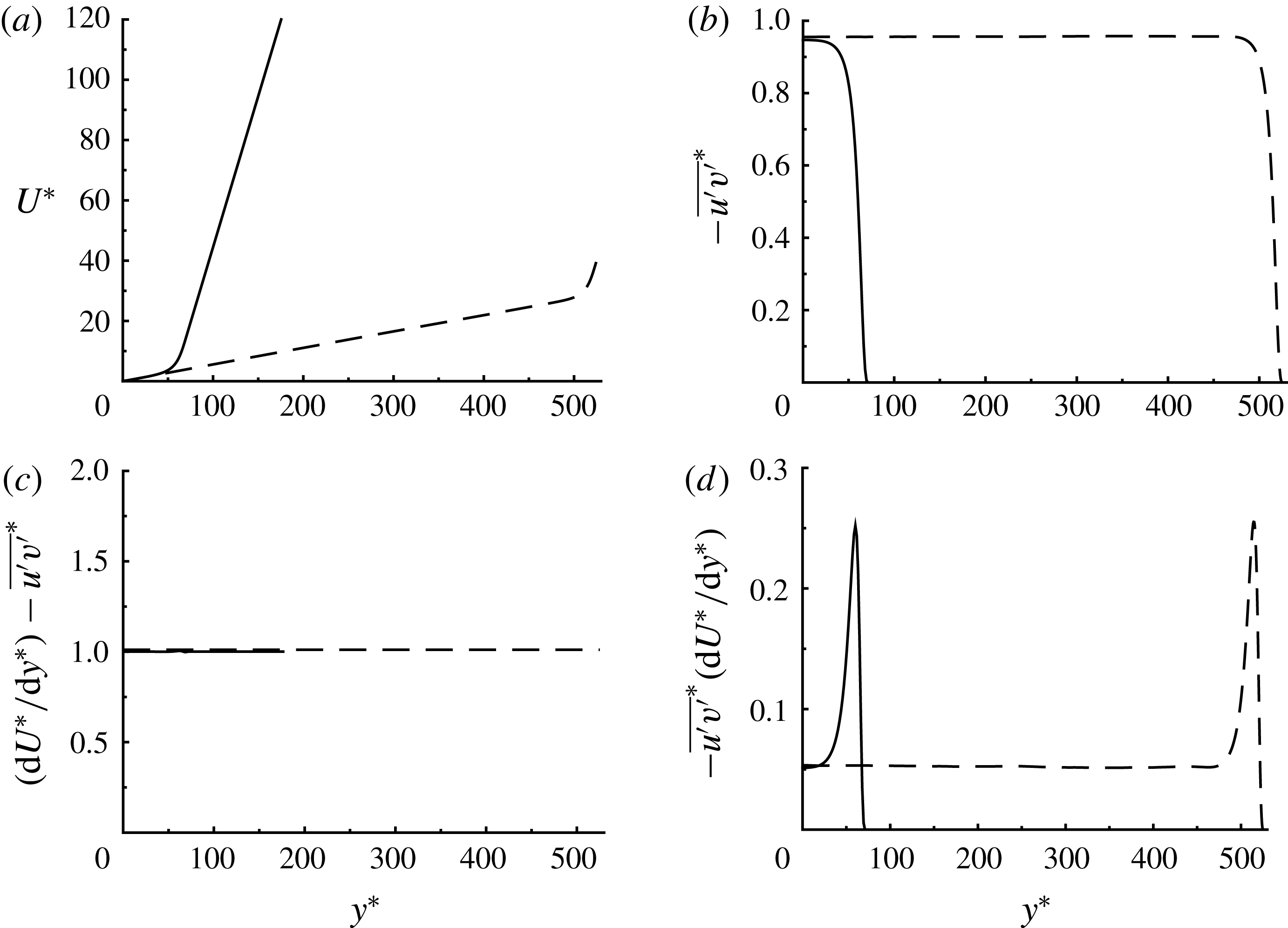
Turbulence statistics for mean-momentum balance and production from the simulation only with the self-sustaining core structures (FSC2) are compared with those of a minimal channel simulation in figure 9. Despite the harsh nature of the applied damping (3.4), the mean shear rate, Reynolds shear stress and turbulence production in the core region (
 $y^{\ast }<30\sim 40$
) of the FSC2 simulation still show reasonably good agreement with those of the full minimal channel simulation. This suggests that the dynamics of the structures in the core region is not significantly disrupted by damping of the structures at
 $|y^{\ast }|>70$
. Application of the damping (3.4) is also found to make the mean shear rate
 $\text{d}U^{\ast }/\text{d}y^{\ast }$
rapidly change for
 $50\lesssim y^{\ast }\lesssim 70$
(figure 9
a), where the Reynolds shear stress rapidly decays (figure 9
b) to satisfy the mean-momentum balance (2.2) (figure 9
c). In this location, turbulence production also exhibits a large peak (figure 9
d), and, interestingly, its peak value appears to be remarkably similar to what is observed in the near-wall region, where the Reynolds shear stress also decays rapidly due to the no-slip boundary condition (see the dashed line in figure 9
d around
 $y^{\ast }\simeq 500$
). A detailed discussion on this observation will be given in § 4.1.
Temporal evolution of flow field in the core region (
 $0\leqslant y^{\ast }\leqslant 70$
) from the FSC2 simulation: (a) time trace of
 $E_{u}^{\ast }$
(solid) and
 $E_{v}^{\ast }$
(dashed); (b) magnification of (a) for
 $t^{\ast }\in [1335,1597]$
; (c–f) the corresponding flow visualisation. In (c–f), the red and blue iso-surfaces indicate
 ${u^{\prime }}^{\ast }=-2.5$
and
 ${v^{\prime }}^{\ast }=0.8$
, respectively.

Temporal evolution of the flow structures in the FSC2 simulation is shown in figure 10. The time trace of
 $E_{u}^{\ast }$
and
 $E_{v}^{\ast }$
in the FSC2 simulation also exhibits temporal oscillations, and their time scale appears to be roughly at
 $T^{\ast }\simeq 200\sim 300$
, not very different from that observed in figure 6 (figure 10
a). The temporal oscillations of
 $E_{u}^{\ast }$
and
 $E_{v}^{\ast }$
also show a phase difference (figure 10
b). Visualisation of the instantaneous flow fields along the different phase in a single oscillation period reveals that the motions in the FSC2 simulation also seem to undergo the SSP/VWI, similarly to the observation made in figure 6. The strong wall-normal velocity structures (figure 10
c) highly amplify a streaky structure (figure 10
d). The amplified streak subsequently meanders along the streamwise direction (figure 10
e), resulting in its breakdown with regeneration of the wall-normal velocity structure (figure 10
f).
Comparison of auto- and cross-correlation functions from (a,c,e) FSC2 and (b,d,f) SC2 simulations: (a,b)
 $C_{uu}$
,
 $C_{vv}$
,
 $C_{ww}$
; (c,d)
 $C_{uv}$
,
 $C_{uw}$
,
 $C_{vw}$
; (e,f)
 $C_{0u}$
,
 $C_{0v}$
,
 $C_{1v}$
.
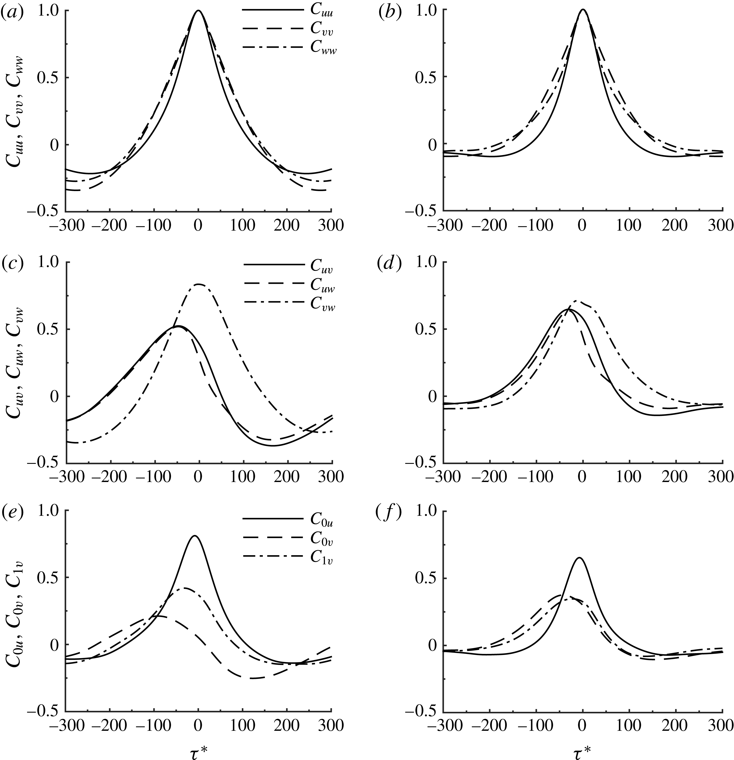
To obtain a more quantitative comparison between the dynamics of the FSC2 and SC2 simulations, auto- and cross-correlations of the time-dependent variables such as those defined in (3.2) are examined as in, for example, Hwang & Bengana (Reference Hwang and Bengana2016). Here, we also introduce two additional variables:
 $$\begin{eqnarray}E_{0}^{\ast }=\frac{1}{l_{y}^{\ast }}\int _{0}^{l_{y}^{\ast }}(|\hat{u} ^{\ast }(y;k_{x},k_{z})|^{2}+|\hat{v}^{\ast }(y;k_{x},k_{z})|^{2}+|{\hat{w}}^{\ast }(y;k_{x},k_{z})|^{2})\,\text{d}y,\end{eqnarray}$$
for
 $k_{x}=0$
and
 $k_{z}=2\unicode[STIX]{x03C0}/L_{z}$
, and
 $$\begin{eqnarray}E_{1}^{\ast }=\frac{1}{l_{y}^{\ast }}\int _{0}^{l_{y}^{\ast }}(|\hat{u} ^{\ast }(y;k_{x},k_{z})|^{2}+|\hat{v}^{\ast }(y;k_{x},k_{z})|^{2}+|{\hat{w}}^{\ast }(y;k_{x},k_{z})|^{2})\,\text{d}y,\end{eqnarray}$$
for
 $k_{x}=2\unicode[STIX]{x03C0}/L_{x}$
and
 $k_{z}=2\unicode[STIX]{x03C0}/L_{z}$
, where
 $E_{0}^{\ast }$
represents energy of the elongated motion extending over the entire streamwise domain, while
 $E_{1}^{\ast }$
measures the strength of wavy meandering motion (i.e. streak instability). The cross-correlation functions are subsequently computed following the definition in (3.3).
Figure 11 compares a number of different auto- and cross-correlations computed from the FSC2 simulation with those from the SC2 simulation. The autocorrelations from both FSC2 (figure 11
a) and SC2 simulations (figure 11
b) show their tails reaching zero at
 $\unicode[STIX]{x1D70F}^{\ast }\simeq \pm 100\sim \pm 150$
, indicating that the turn-over time scale of the structures in both of the cases would be
 $T^{\ast }\simeq 200\sim 300$
, consistent with the observations in figures 6 and 10. The cross-correlations between
 $E_{u}^{\ast }$
,
 $E_{v}^{\ast }$
and
 $E_{w}^{\ast }$
of both cases (figure 11
c,d) reveal that the wall-normal and spanwise velocities are well correlated to each other, indicating the presence of streamwise roll-like structures (
 $C_{vw}$
in figure 11
c,d). On the other hand,
 $E_{v}^{\ast }$
and
 $E_{w}^{\ast }$
exhibit a phase difference from
 $E_{u}^{\ast }$
: the peaks of
 $C_{uv}$
and
 $C_{uw}$
in both cases appear at
 $\unicode[STIX]{x1D70F}^{\ast }\simeq -60\sim -40$
. The cross-correlations of
 $E_{u}^{\ast }$
with
 $E_{0}^{\ast }$
in both cases (
 $C_{0u}$
in figure 11
e,f) show a large value around
 $\unicode[STIX]{x1D70F}^{\ast }\simeq 0$
. This implies that
 $E_{u}^{\ast }$
represents the elongated motion of the streamwise velocity, indicating the streaky motion in figures 6 and 10. For this reason, the cross-correlation between
 $E_{0}^{\ast }$
and
 $E_{v}^{\ast }$
in both cases (
 $C_{0v}$
in figure 11
e,f) exhibits a peak at
 $\unicode[STIX]{x1D70F}^{\ast }\simeq -80\sim -50$
, similarly to
 $C_{uv}$
. Finally, the cross-correlation between
 $E_{1}^{\ast }$
and
 $E_{v}^{\ast }$
in both cases (
 $C_{1v}$
in figure 11
e,f) reveals its peak location around
 $\unicode[STIX]{x1D70F}^{\ast }\simeq -40\sim -20$
. This indicates that a streamwise meandering motion consistently appears before the streamwise roll-like structures are generated.
Overall, the auto- and cross-correlations from the FSC2 and SC2 simulations show qualitatively good agreement with each other, suggesting that the dynamics of the self-sustaining structures in the FSC2 case is not very different from that in the SC2 case. Furthermore, the correlations also suggest that there exists a statistically cyclic process in the core region of both simulations, which occurs in the following order:
 $$\begin{eqnarray}E_{u}^{\ast }~\& ~E_{0}^{\ast }\longrightarrow E_{1}^{\ast }\longrightarrow E_{v}^{\ast }~\& ~E_{w}^{\ast }\longrightarrow E_{u}^{\ast }~\& ~E_{0}^{\ast },\end{eqnarray}$$
with the turn-over time scale,
 $T^{\ast }\simeq 200\sim 300$
. The fluid motion associated with
 $E_{u}^{\ast }$
and
 $E_{0}^{\ast }$
indicates an elongated streamwise velocity structure, very likely to be a ‘streak’, and
 $E_{1}^{\ast }$
indicates its streak meandering motion is presumably caused by a streak instability. The streak instability process occurs before the generation of streamwise roll-like structures represented by
 $E_{v}^{\ast }$
and
 $E_{w}^{\ast }$
. The statistical evidence in figure 11 therefore firmly indicates the existence of the SSP/VWI in the core region of the SC2 simulation. Here, it should be stressed that the existence of the SSP/VWI in the SC2 simulation is not limited only to the core region. The observed dynamics in the core region should be invariant under a wall-normal translation, thus it has to be relevant to other wall-normal locations, except the near-wall region where the translational invariance would be broken due to the no-slip boundary condition. However, also in the near-wall region, it is well understood that the SSP/VWI is the main driving mechanism of turbulence (Jiménez & Moin Reference Jiménez and Moin1991; Jiménez & Pinelli Reference Jiménez and Pinelli1999). In summary, we conclude that the SSP/VWI is the dominant mechanism of turbulence production at all wall-normal locations in the present minimal-span simulations.
4 Discussion
An important outcome of the present minimal-span numerical simulations for turbulent Couette flow is that they enable us to generate a uniform shear flow in the bulk turbulent region, unaffected by the wall region. In particular, the minimal-span simulations enable us to isolate and discuss processes at the Kolmogorov scale in the bulk. We have shown that there indeed exists a turbulence production mechanism at the Kolmogorov microscale in the bulk region of turbulent Couette flow. The related eddies essentially originate from the mean shear existing at every wall-normal location, and do not rely on the presence of the wall. In this respect, the present study is consistent with Mizuno & Jiménez (Reference Mizuno and Jiménez2013), where a scaling procedure is used to eliminate wall effects. Statistical evidence also firmly indicates that the turbulence production mechanism is supported by the SSP/VWI. This suggests that the self-similar invariant solutions found by recent studies (Blackburn et al. Reference Blackburn, Hall and Sherwin2013; Deguchi Reference Deguchi2015; Eckhardt & Zammert Reference Eckhardt and Zammert2016) may be relevant to turbulence production observed in the present study.
It is yet to be clarified whether the eddies observed in the present study may be associated with the turbulent cascade. We note that the eddies involved in the energy cascade, and dissipation of a typical turbulent flow at high Reynolds numbers, are expected to be ‘driven’ by the energy transferred from ‘large scale’ due to the balance between turbulence production and dissipation (Kolmogorov Reference Kolmogorov1941, Reference Kolmogorov1991). However, the eddies in the present minimal-span simulation emerge in the absence of any large scales by taking energy directly from the mean shear. Further, the Kolmogorov-scale eddies in the present study are not isotropic, unlike the hypothesis of Kolmogorov (Reference Kolmogorov1941, Reference Kolmogorov1991), although the hypothesis itself may not be fully justified yet. Finally, it is important to point out that the self-sustaining eddies in the present study are still much larger than those associated with turbulence dissipation, even though their size scales with the Kolmogorov microscale. Indeed, the typical size of the dissipative eddies at the Kolmogorov scale is only
 $O(\unicode[STIX]{x1D702})$
(Jiménez & Wray Reference Jiménez and Wray1998), much smaller than the eddies in the present study at
 $O(100\unicode[STIX]{x1D702})$
.
Taking these observations together, the self-sustaining eddies at the Kolmogorov microscale observed in the present study are unlikely to be relevant for full-scale turbulent flows at high Reynolds number. Instead, these eddies are more relevant for flow at transitional Reynolds numbers in the presence of uniform shear: the small size of the eddies at
 $O(100\unicode[STIX]{x1D702})$
, originating from artificial restriction of the spanwise length scale by the periodic boundary condition, reduces the characteristic Reynolds number to be
 $Re_{c}(\equiv u_{\unicode[STIX]{x1D70F}}(100\unicode[STIX]{x1D702})/\unicode[STIX]{x1D708})=100$
, resulting in a transitional flow where there is little separation between the length scales of turbulence production and dissipation. We note that the same appears to be true for turbulence in the near-wall region (i.e. buffer layer): the length scale of turbulence production is artificially restricted by the distance from the wall due to the no-slip boundary condition, and the smallest possible length scale of turbulence would therefore be given by the balance between the associated production and viscous dissipation. This explains why the viscous inner length scale is the same as the near-wall Kolmogorov length scale. The present study implies that such a phenomenon may occur whenever the size of the eddies is artificially restricted, for example, by a boundary condition.
4.1 Uniform shear versus near-wall turbulence
Uniform shear turbulence has often been compared with near-wall turbulence (Lee, Kim & Moin Reference Lee, Kim and Moin1990; Sekimoto, Dong & Jiménez Reference Sekimoto, Dong and Jiménez2016). Here we are able to make a direct comparison between them, while maintaining all the other conditions, such as applied shear stress and horizontal boundary conditions, to be exactly the same. In the present study, we have shown that the eddies in the bulk region are generated by the same mechanism as in near-wall turbulence, i.e. the SSP/VWI (figure 6) (Hamilton et al.
Reference Hamilton, Kim and Waleffe1995; Jiménez & Pinelli Reference Jiménez and Pinelli1999; Schoppa & Hussain Reference Schoppa and Hussain2002). The eddy turn-over time scale of the bulk region is also found to be
 $T^{\ast }\simeq 200{-}300$
at least with
 $L_{x}^{\ast }\simeq 400$
(figure 7), and this value corresponds very well to the typical near-wall time scale
 $T^{+}\simeq 200{-}300$
(Jiménez et al.
Reference Jiménez, Kawahara, Simens, Nagata and Shiba2005). However, the near-wall turbulence appears to be more anisotropic than uniform shear turbulence (figures 3 and 4): in particular, the streamwise turbulence intensity of near-wall turbulence is much stronger than that for the uniform shear case (figure 3), and the related streaky structures also appear to be twice as elongated in the streamwise direction (figures 4 and 14). This implies that the dynamics of coherent structures in near-wall turbulence is very similar to that in uniform shear turbulence, but their statistical features are significantly different.
One such important statistical difference is the large value of production in the near-wall turbulence, the peak value of which is about four to five times greater than that of uniform shear turbulence (figure 2
d). In fact, this is a very common feature of the near-wall region in any simulation of wall-bounded shear flows, and, for many years, it has led to a misunderstanding that the near-wall region is the most vigorous location where turbulence production is dominant (see also Marusic et al.
Reference Marusic, McKeon, Monkewitz, Nagib, Smits and Sreenivasan2010, for a further discussion). However, the numerical experiments in the present study suggest that the emergence of such a peak in the near-wall turbulence production may be a local ‘transitional’ effect simply caused by the no-slip boundary condition. In the near-wall region of the present minimal-span simulation, the no-slip condition leads
 $-\overline{u^{\prime }v^{\prime }}^{\ast }$
to decay rapidly on approaching the wall (figure 2
b). Since the mean-momentum balance (2.2) needs always to be satisfied, this results in a rapid increase of
 $\text{d}U^{\ast }/\text{d}y^{\ast }$
in the near-wall region. Here, we note that the value of
 $-\overline{u^{\prime }v^{\prime }}^{\ast }\,(\text{d}U^{\ast }/\text{d}y^{\ast })$
subject to (2.2) mathematically reaches its maximum when
 $\text{d}U^{\ast }/\text{d}y^{\ast }=-\overline{u^{\prime }v^{\prime }}^{\ast }=0.5$
. Since
 $-\overline{u^{\prime }v^{\prime }}^{\ast }\simeq 0.93$
in the bulk region, the only place where
 $-\overline{u^{\prime }v^{\prime }}^{\ast }=0.5$
is physically possible would be the near-wall region, where the maximum of
 $-\overline{u^{\prime }v^{\prime }}^{\ast }\,(\text{d}U^{\ast }/\text{d}y^{\ast })$
indeed emerges at
 $y^{+}\simeq 10$
in the present minimal-span simulations (see also figure 14
a). It is important to mention that the same phenomenon also occurs in the FSC2 simulation, where all the structures are artificially damped out except those in the core region. In the FSC2 simulation, the location of
 $-\overline{u^{\prime }v^{\prime }}^{\ast }=0.5$
is given by
 $|y^{\ast }|\simeq 60$
due to the applied artificial damping (figure 9
b), and
 $-\overline{u^{\prime }v^{\prime }}^{\ast }\,(\text{d}U^{\ast }/\text{d}y^{\ast })$
reaches the maximum at this location. This implies that the emergence of the large peak of
 $-\overline{u^{\prime }v^{\prime }}^{\ast }\,(\text{d}U^{\ast }/\text{d}y^{\ast })$
in both of the SC2 and FSC2 simulations is essentially due to the decaying Reynolds shear stress subject to (2.2), indicating that the large value of production in the near-wall turbulence may be a local effect caused by the no-slip boundary condition.
It should also be stressed that this feature is not necessarily limited to the present minimal-span simulations of turbulent Couette flow – it appears to be generic, at least for any parallel internal wall-bounded shear flows. For example, the mean-momentum balance in a pressure-driven channel flow (e.g. Tennekes & Lumley Reference Tennekes and Lumley1967) is given by
 $$\begin{eqnarray}\frac{\text{d}U^{+}}{\text{d}y^{+}}-\overline{u^{\prime }v^{\prime }}^{+}=1-\frac{y^{+}}{Re_{\unicode[STIX]{x1D70F}}},\end{eqnarray}$$
and the same expression would be easily found for turbulent pipe flow, as the viscous inner length scale is much smaller than that associated with the boundary curvature at high Reynolds numbers. In the limit of
 $Re_{\unicode[STIX]{x1D70F}}\rightarrow \infty$
, equation (4.1) in the near-wall region (say
 $y^{+}\leqslant 100$
) becomes the same as (2.2) because the viscous inner scales are identical to the related Kolmogorov scales in the near-wall region. It is important to remember that both
 $\text{d}U^{+}/\text{d}y^{+}$
and
 $-\overline{u^{\prime }v^{\prime }}^{+}$
in the near-wall region of wall-bounded turbulent shear flow scale very well in the viscous inner units, unlike other statistics such as streamwise and spanwise turbulence intensities, and that they remain constant even if the Reynolds number is sufficiently high (see e.g. the DNS data by Lee & Moser Reference Lee and Moser2015). Therefore, the maximum value of turbulence production in near-wall turbulence is also expected to be around
 $y^{+}\simeq 10$
, consistent with the early observations (Tennekes & Lumley Reference Tennekes and Lumley1967), and it should scale very well in the inner units.
4.2 How large is the turbulence production at Kolmogorov microscale?
An important outcome of the present study is that turbulence production exists at the Kolmogorov microscale. This mechanism is essentially driven by the local mean shear. However, the reason that this mechanism is unveiled here is essentially because larger eddies are artificially removed. From this viewpoint, it is not very clear whether this turbulence production mechanism would also be active in the presence of larger eddies: indeed, the spectra in full DNS by Pirozzoli et al. (Reference Pirozzoli, Bernardini and Orlandi2014) do not show any strong turbulent kinetic energy in the region where the production by Kolmogorov microscale is expected (see figure 8 in Pirozzoli et al. Reference Pirozzoli, Bernardini and Orlandi2014). This implies that the production mechanism discovered in the present study may not be very active in the presence of the eddies at all the possible scales.
Variation of skin-friction coefficient with
 $Re$
: ——, empirical fit by Robertson (Reference Robertson1959),
 $C_{f}=0.424(\ln Re)^{-2}$
; ●, DNS by Pirozzoli et al. (Reference Pirozzoli, Bernardini and Orlandi2014); ▫, LC cases; ♢, SC cases.
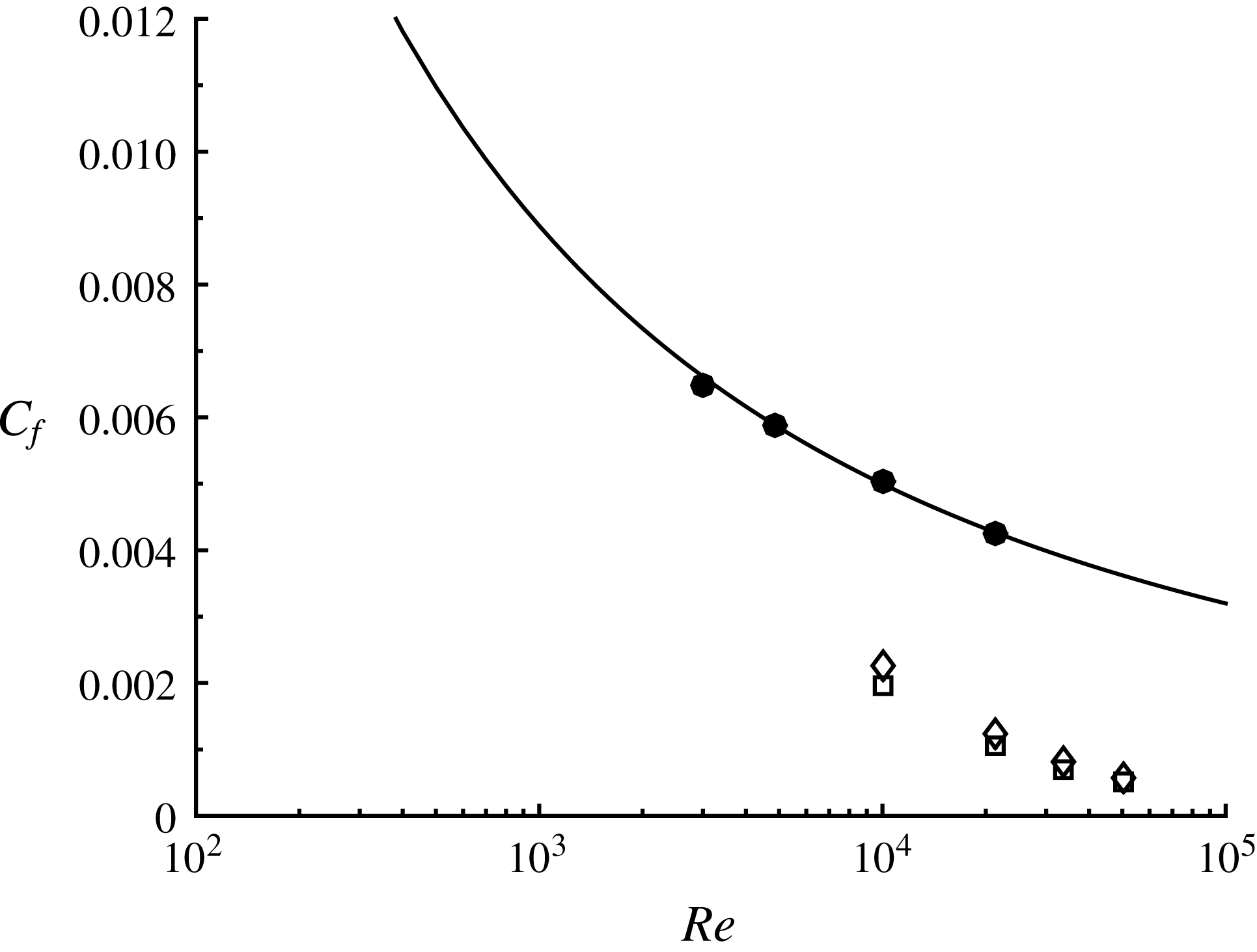
It is also useful to compute how much energy is dissipated in the present minimal-span simulation, in comparison to that in full simulations. This can be easily obtained by computing skin-friction drag (e.g. Kawahara & Kida Reference Kawahara and Kida2001). Figure 12 shows variation of skin-friction coefficient of full simulations (Pirozzoli et al.
Reference Pirozzoli, Bernardini and Orlandi2014) and the present minimal-span simulations on increasing the Reynolds number. As in Hwang (Reference Hwang2013) and de Giovanetti et al. (Reference de Giovanetti, Hwang and Choi2016) for pressure-driven turbulent channel flows, the removal of the motions, the spanwise size of which is greater than
 $\unicode[STIX]{x1D706}_{z}^{\ast }>100{-}140$
, leads to a significant amount of skin-friction reduction. Also, the difference of the skin friction generated by the minimal-span simulations from that by full simulations increases, as the Reynolds number increases. This observation also suggests that the production by the Kolmogorov microscale in the present numerical experiment is much smaller than that by the full simulation. In this respect, it is finally worth mentioning that the Reynolds shear-stress cospectra in a full-scale turbulent flow at high Reynolds numbers were shown to decay with a
 $-7/3$
power law, before it reaches the dissipation range of the spectra (Lumley Reference Lumley1967; Saddoughi & Veeravallit Reference Saddoughi and Veeravallit1994). This indicates that the turbulence production by the eddies at the Kolmogorov microscale would also be insignificant and very small in a full-scale turbulent flow.
4.3 Above the near-wall region in the minimal unit simulation
Finally, the present study provides a better understanding for the previous minimal-span simulations for pressure-driven channel flow (e.g. Jiménez & Moin Reference Jiménez and Moin1991; Jiménez & Pinelli Reference Jiménez and Pinelli1999; Hwang Reference Hwang2013). All of these studies have repeatedly reported the presence of a non-negligible amount of turbulent fluctuations above the near-wall region in the minimal-span simulations, even though the spanwise computational domain is not large enough to resolve the large energy-carrying eddies in the logarithmic and outer regions. An explanation for the emergence of such turbulent fluctuations above the near-wall region in the minimal-span simulations was initially proposed by Jiménez & Pinelli (Reference Jiménez and Pinelli1999), and it starts from turbulence production in the logarithmic region:
 ${\mathcal{P}}\sim u_{\unicode[STIX]{x1D70F}}^{3}/y$
. Since the production is roughly balanced with dissipation in the logarithmic region, the decaying vorticity fluctuation in the wall-normal direction would be given, such that
 $\unicode[STIX]{x1D714}\sim y^{-1/2}$
from
 ${\mathcal{P}}\sim \unicode[STIX]{x1D708}\unicode[STIX]{x1D714}^{2}$
. However, in the minimal-span simulation, the integral length scale above the near-wall region is artificially restricted to be
 $L_{z}$
. Therefore, the balance between production and dissipation yields
 $\unicode[STIX]{x1D714}\sim L_{z}^{-1/2}$
, providing a sound reason for the non-negligible turbulent fluctuation above the near-wall region in the minimal-span simulation.
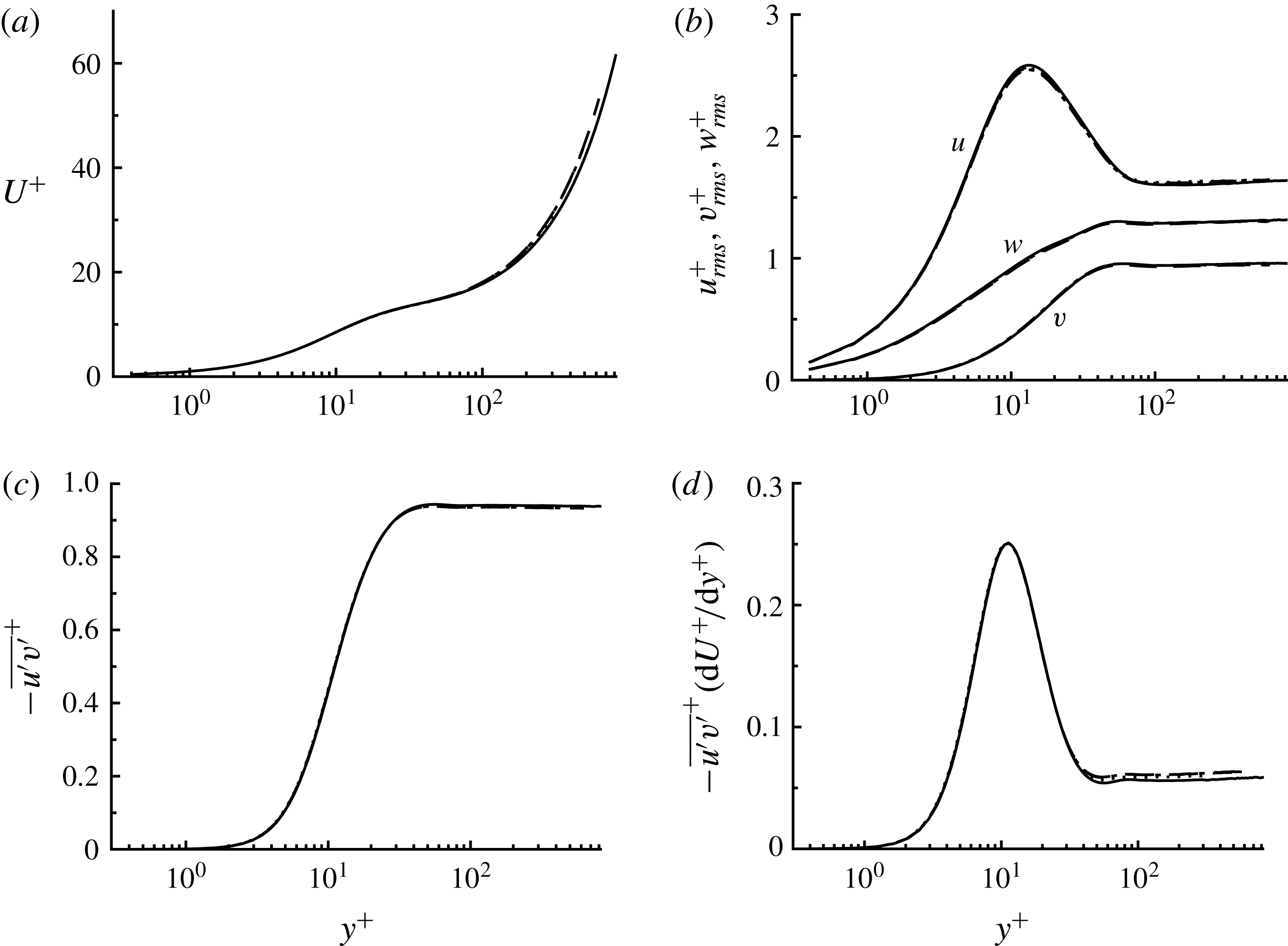
Near-wall turbulence statistics: (a)
 $U^{+}(y^{+})$
, (b)
 $u_{rms}^{+}(y^{+})$
,
 $v_{rms}^{+}(y^{+})$
,
 $w_{rms}^{+}(y^{+})$
, (c)
 $-\overline{u^{\prime }v^{\prime }}^{+}(y^{+})$
, (d)
 $-\overline{u^{\prime }v^{\prime }}^{+}(y^{+})(\text{d}U^{+}/\text{d}y^{+})$
.
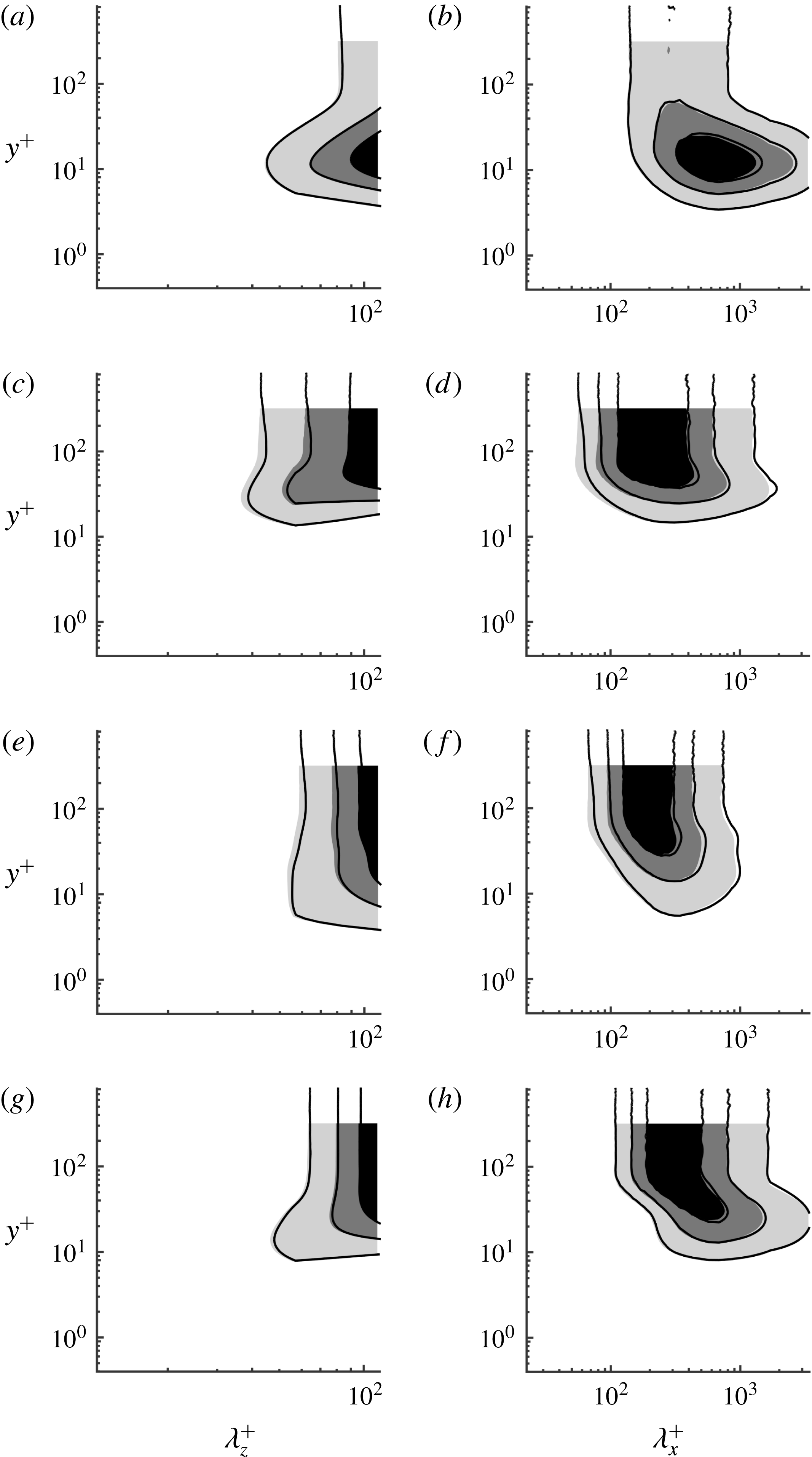
Premultiplied one-dimensional (a,c,e,g) spanwise and (b,d,f,h) streamwise wavenumber spectra of (a,b) streamwise velocity, (c,d) wall-normal velocity, (e,f) spanwise velocity and (g,h) Reynolds shear stress. Here: shaded, LC1; solid, LC4. The contour levels are 0.25, 0.5 and 0.75 times of each of the maximum.
The present study highlights that this explanation should be based upon the assumption that the production in the minimal-span simulation does not originate from the near-wall region but from the local mean shear. In the case of Couette flow, the uniform mean shear in the bulk region makes the spanwise domain size
 $L_{z}$
the precise integral length scale in the bulk region, thereby resulting in turbulence statistics constant in the wall-normal direction. On the other hand, in the case of pressure-driven channel flow, the size of the spanwise domain does not fully represent the integral length scale in the bulk region, as the mean shear is essentially the outcome of the applied pressure gradient – the mean shear in this case decays on approaching from the near-wall to the core region. Therefore, the production mechanism and the resulting turbulent fluctuations are expected to be gradually weakened, as the wall-normal location moves from the near-wall to the outer region, and this is consistent with the turbulence statistics reported by Hwang (Reference Hwang2013). However, it is also important to mention that there should exist eddies, similar to those observed in the bulk region of the present study, at least just above the near-wall region at sufficiently high Reynolds number, because the mean-momentum balance (4.1) of the pressure-driven channel flow would be identical to (2.2) in the limit of
 $Re_{\unicode[STIX]{x1D70F}}\rightarrow \infty$
in this region. Indeed, the eddy structures and their length scales above the near-wall region in a minimal-span pressure-driven channel flow (Hwang Reference Hwang2013) are remarkably similar to those in the bulk region of the present study. Lastly, it should be stressed that this may indicate the existence of invariant solutions associated with these fluctuations in a pressure-driven channel flow, as in the present Couette flow. However, to the best of our knowledge, the discovery of such invariant solutions is yet to be reported.
Acknowledgements
Q.Y. would like to thank China Scholarship Council for financial support. Y.H. was supported by the Engineering and Physical Sciences Research Council (EPSRC) in the UK (EP/N019342/1). We also gratefully acknowledge helpful discussions with Professor J. C. Vassilicos and Dr K. Deguchi.
Appendix. Near-wall turbulence statistics of the spanwise-minimal Couette flow
The near-wall turbulence statistics of all the LC simulations are reported here. Figure 13 reports first- and second-order turbulence statistics scaled by
 $\unicode[STIX]{x1D6FF}_{\unicode[STIX]{x1D708}}$
, with which the wall-normal coordinate is given by
 $y^{+}=(y+h)/\unicode[STIX]{x1D6FF}_{\unicode[STIX]{x1D708}}$
. Consistently with Hwang (Reference Hwang2013), all the turbulent statistics show very good agreement at all the Reynolds numbers considered, and they are almost indistinguishable in the near-wall region. One-dimensional spectra of all the velocity components and the Reynolds shear stress are also inspected, as shown in figure 14. Comparison of the spectra from the lowest and the highest Reynolds number clearly suggests that the near-wall turbulence statistics completely scale in the viscous inner units. The spectra also very well characterise the typical behaviour of near-wall turbulence (see also Hwang Reference Hwang2013, for further details) – in particular, the streamwise wavenumber spectra of the streamwise velocity shows a peak at
 $\unicode[STIX]{x1D706}_{x}^{+}\simeq 600$
and
 $y^{+}\simeq 15$
(figure 14
b), indicating the near-wall streaks, while those of the wall-normal and spanwise velocities exhibit peaks at
 $\unicode[STIX]{x1D706}_{x}^{+}\simeq 200\sim 300$
and
 $y^{+}\simeq 500$
, representing the quasi-streamwise vortices (Jeong et al.
Reference Jeong, Benney, Schoppa and Kim1997).



