1 Introduction
Thin viscous fluid layers driven by gravity occur widely in nature and industry. The most commonly studied examples are those where the dominant resistance to flow stems from the drag or viscous shear stresses caused by contact with an underlying surface or viscous fluid (e.g. Lister & Kerr Reference Lister and Kerr1989). However, there are many important examples of so-called extensional flows, which arise when a viscous film flows along a solid or fluid interface with small or negligible drag and the dominant resistance to flow is from extension (stretching). Examples include the flow of glacial ice shelves over the ocean (Weertman Reference Weertman1957), of float glass over molten tin (Howell Reference Howell1994), of crude oil over water (DiPietro & Cox Reference DiPietro and Cox1979) and of certain regions of the Earth’s crust over the mantle (Copley & McKenzie Reference Copley and McKenzie2007). Studies of extensional flows to date have concentrated on horizontally one-dimensional and axisymmetric cases, for which the dynamics are controlled primarily by buoyancy and the resistance to extension in the direction of flow. The aim of this paper is to investigate dynamical regimes that arise when an extensional flow is subject to lateral stresses due to confining boundaries.
My main motivation is to elucidate the general dynamical principles underlying the flow of floating glaciers, or ice shelves, which occur when a glacial ice sheet flows into the ocean and floats under the influence of buoyancy. The archetypal ice sheet of this kind, known as a marine ice sheet, is the West Antarctic Ice Sheet (WAIS), which contains a grounded component that sits predominantly on bedrock below sea level (Bamber et al. Reference Bamber, Riva, Vermeersen and LeBrocq2009). As it flows outwards from the centre of Antarctica, there is a critical location, called the grounding line, at which the WAIS detaches from the underlying bedrock and forms a floating ice shelf. This extends downstream of the grounding line and eventually fractures at its calving front to form icebergs. The glacial creep of ice can be modelled as a viscous shear-thinning fluid (Cuffey & Paterson Reference Cuffey and Paterson2010). Therefore, an ice shelf forms a thin layer of viscous fluid that floats on the effectively inviscid ocean water. The tangential stresses exerted by the air above it and ocean underneath it are both negligible compared to the viscous stresses within the ice shelf, creating the conditions for an extensional flow (Weertman Reference Weertman1957).
The dynamics of ice shelves and other extensional flows can be described by a set of depth-integrated horizontally two-dimensional equations (DiPietro & Cox Reference DiPietro and Cox1979; Morland Reference Morland1987; Howell Reference Howell1994; Pegler & Worster Reference Pegler and Worster2012). These equations have been considered primarily in one-dimensional and axisymmetric situations, including constant-volume releases (Pegler, Lister & Worster Reference Pegler, Lister and Worster2012) and flows arising from localized injections (DiPietro & Cox Reference DiPietro and Cox1979; Robison, Huppert & Worster Reference Robison, Huppert and Worster2010; Pegler & Worster Reference Pegler and Worster2012). The one-dimensional case of the equations, which describes a pure balance between extensional stresses in the direction of flow and buoyancy, has been developed and used widely as a simple model of an unconfined ice shelf (Morland & Shoemaker Reference Morland and Shoemaker1982; Van der Veen Reference Van der Veen1983; MacAyeal & Barcilon Reference MacAyeal and Barcilon1988). In this idealized regime, the flow of an ice shelf is controlled primarily by input conditions and is independent of the position of its calving front. With fluid introduced at a constant rate, it is found that the one-dimensional flow develops concave surfaces with a frontal position that accelerates with time (as
 $t^{2}$
for Newtonian fluid, for example). This simplified regime driven by buoyancy and resisted purely by extension is based on the assumption that the stresses arising from any lateral contact play a negligible role.
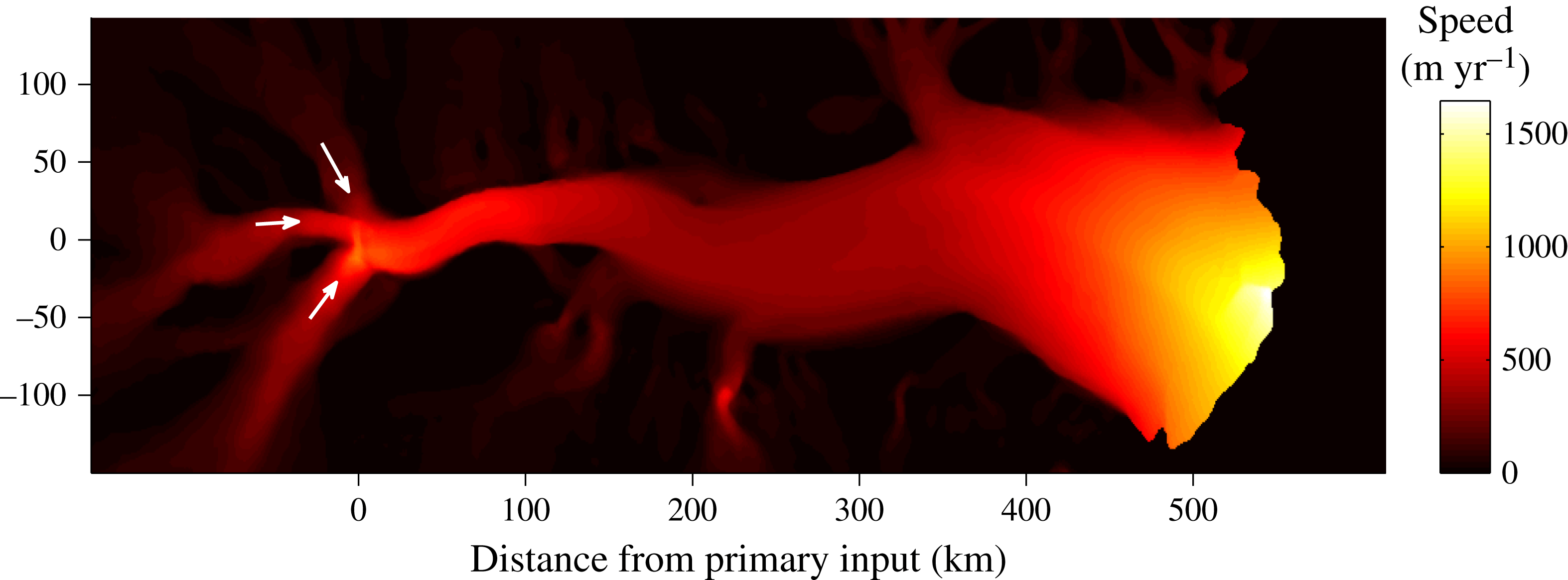
However, contact between a floating layer of fluid and confining lateral boundaries is common in physical situations. Many ice shelves, for example, contain significant regions of lateral contact with land or near-stationary grounded ice. The Amery Ice Shelf, which flows in a channel approximately 550 km long and 50–200 km wide, provides an archetype. The length of contact between the largest ice shelves, the Ross and Ronne Ice Shelves, and grounded lateral ice is comparable to their transverse width. Velocimetric data (Rignot, Mouginot & Scheuchl Reference Rignot, Mouginot and Scheuchl2011) show significant transverse shear at the margins of these ice shelves, indicative of sidewall stresses. For ice shelves with only slight lateral contact, a purely extensional model may be most relevant. Conversely, significant lateral contact may lead to a regime dominated by a balance between lateral stresses and buoyancy. While these two limiting balances are possible, to date there has been no detailed analysis of the fluid-mechanical regimes they produce, nor any classification of the parameter values for which they occur.
Several glaciological studies have considered the two-dimensional extensional flow equations in simulations of confined ice shelves (e.g. MacAyeal et al. Reference MacAyeal, Rommelaere, Huybrechts, Hulbe, Determann and Ritz1996; Goldberg, Holland & Schoof Reference Goldberg, Holland and Schoof2009; Gudmundsson et al. Reference Gudmundsson, Krug, Durand, Favier and Gagliardini2012). These predict features of the flows, including their plug-like cross-channel profiles and sheared margins. Others have used quasi-one-dimensional (flow-line) models that either specify a lateral drag or parametrize it in terms of a centreline velocity (e.g. MacAyeal Reference MacAyeal1989; Van der Veen Reference Van der Veen1999; Dupont & Alley Reference Dupont and Alley2005). Such models allow for both extensional and shear stresses simultaneously. However, these studies do not present detailed conclusions relating to physical balances and flow regimes. A recent development relating specifically to flow at the calving front has been to provide a scaling relationship for the flux of ice at the calving front based on the assumption that lateral drag, extensional stresses and buoyancy are comparable (Hindmarsh Reference Hindmarsh2012; Wearing, Hindmarsh & Worster Reference Wearing, Hindmarsh and Worster2015). Similar scales arising from the identification of the channel width as the relevant longitudinal length scale were used by Pegler (Reference Pegler2012) in obtaining dimensionless solutions to a two-dimensional model with zero lateral slip. The balance between extension, drag and buoyancy underlying this scaling is qualitatively similar to that which arises at a grounding line separating a drag-dominated grounded ice sheet and a purely extensional ice shelf (Schoof Reference Schoof2007). Likewise, there can be a region far upstream dominated by the resistance due to drag and buoyancy. In the context of laterally confined extensional flows, this balance corresponds to a limiting form of dynamics equivalent to flow in a vertical Hele-Shaw cell (Pegler et al. Reference Pegler, Kowal, Hasenclever and Worster2013).
The objective of this paper is to provide a unified analysis of thin-layer flows arising from the mixture of extensional stresses, lateral stresses and buoyancy. Motivated by the configuration of an ice shelf, I consider the specific case in which fluid is introduced into a confining channel of finite length. The analysis will identify the possible flow regimes and intrinsic scales, obtain time-dependent and steady-state solutions both analytically and numerically, analyse these using analytical and asymptotic methods, and classify the possible flow regimes across the full space of parameters. I also present a new series of laboratory experiments, which I use to determine the full two-dimensional velocity field and to test the theoretical predictions. These involve particle velocimetry of a floating viscous fluid film flowing between sidewalls of finite extent, providing an effective simulation of an ice shelf flowing towards a fixed calving front. The final aim is to map the positions of a selection of ice shelves over the space of geometrical and fluid-mechanical parameters, and thus assess the prevalence of regimes involving sidewall control in the geophysical setting.
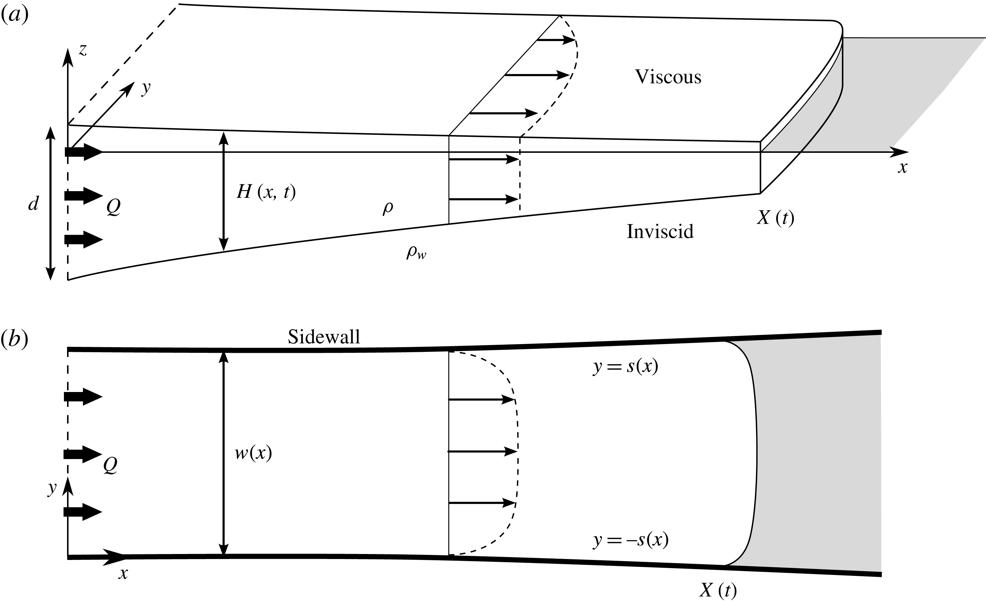
(a) Cross-sectional and (b) plan-view schematics of a viscous fluid film floating on an inviscid fluid and confined laterally by vertical sidewalls.

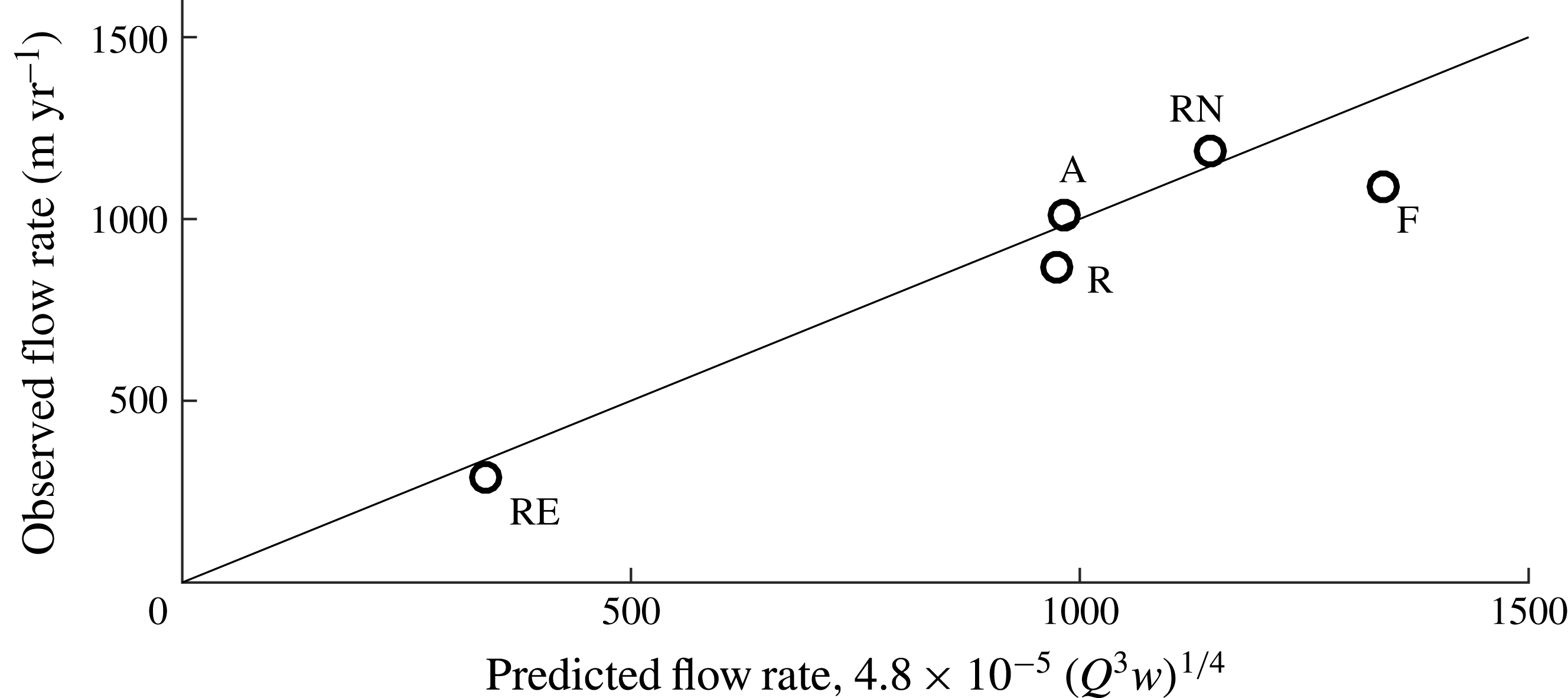
I begin in § 2 by developing a width-integrated form of the two-dimensional extensional flow equation, which distils the dynamics to the key forces involving extension, lateral stresses and buoyancy. The time-dependent and steady-state dynamics are explored in § 3 in the case of Newtonian fluid introduced into a parallel, open-ended channel. My laboratory study is presented in § 4 and the results compared alongside theory. Rheological effects of shear thinning are considered in § 5, as applies to the flow of glacial ice. In § 6, the geophysical classification of ice shelves is presented alongside comparisons between the theoretical prediction for the width-averaged flow rate towards the calving front and data for a selection of ice-shelf systems.
2 General model equations
Consider a layer of viscous fluid of density
 $\unicode[STIX]{x1D70C}$
floating on a body of inviscid fluid of greater density
 $\unicode[STIX]{x1D70C}_{w}>\unicode[STIX]{x1D70C}$
, as illustrated in figure 1. The layer is assumed to lie confined between two vertical sidewalls along
 $y=\pm s(x)$
, forming a channel of width
 $w(x)=2s(x)$
. Let
 $H(\boldsymbol{x},t)$
denote the vertical thickness distribution of the layer at time
 $t$
and horizontal position
 $\boldsymbol{x}\equiv (x,y)$
. A floating layer of fluid will naturally lie in a position of Archimedean flotation in which its upper, free surface
 $z=h(\boldsymbol{x},t)$
is related to its thickness
 $H$
via
 $$\begin{eqnarray}h(\boldsymbol{x},t)=(\unicode[STIX]{x0394}\unicode[STIX]{x1D70C}/\unicode[STIX]{x1D70C}_{w})H(\boldsymbol{x},t),\end{eqnarray}$$
where
 $\unicode[STIX]{x0394}\unicode[STIX]{x1D70C}\equiv \unicode[STIX]{x1D70C}_{w}-\unicode[STIX]{x1D70C}$
is the density difference between the two fluids. Assuming also that the underlying denser fluid exerts negligible stresses on the viscous fluid layer, the leading-order dynamics of the layer can be described by the extensional flow equations,
 $$\begin{eqnarray}\displaystyle & \displaystyle \unicode[STIX]{x1D735}(\unicode[STIX]{x1D707}H\unicode[STIX]{x1D735}\boldsymbol{\cdot }\boldsymbol{u})+\unicode[STIX]{x1D735}\boldsymbol{\cdot }(\unicode[STIX]{x1D707}H\unicode[STIX]{x1D65A})={\textstyle \frac{1}{2}}\unicode[STIX]{x1D70C}g^{\prime }H\unicode[STIX]{x1D735}H, & \displaystyle\end{eqnarray}$$
 $$\begin{eqnarray}\displaystyle & \displaystyle \frac{\unicode[STIX]{x2202}H}{\unicode[STIX]{x2202}t}+\unicode[STIX]{x1D735}\boldsymbol{\cdot }(H\boldsymbol{u})=0, & \displaystyle\end{eqnarray}$$
where
 $\boldsymbol{u}(\boldsymbol{x},t)$
is the horizontal velocity of the layer,
 $\unicode[STIX]{x1D735}$
is the horizontal gradient operator,
 $g^{\prime }\equiv (\unicode[STIX]{x0394}\unicode[STIX]{x1D70C}/\unicode[STIX]{x1D70C}_{w})g$
is the reduced gravity,
 $\unicode[STIX]{x1D707}(\boldsymbol{x},t)$
is the effective viscosity (uniform and constant for a Newtonian fluid) and
 $\unicode[STIX]{x1D65A}\equiv 1/2[\unicode[STIX]{x1D735}\boldsymbol{u}+(\unicode[STIX]{x1D735}\boldsymbol{u})^{\text{T}}]$
is the horizontal rate-of-strain tensor (see DiPietro & Cox (Reference DiPietro and Cox1979), MacAyeal (Reference MacAyeal1989) or Pegler & Worster (Reference Pegler and Worster2012) for derivations of these equations). Equation (2.2) describes a balance between the driving gradient in depth-integrated hydrostatic pressure on the right-hand side and the divergence of depth-integrated stresses due to vertical extension and deviatoric deformations on the left-hand side. Motivated by application to glaical flow, I consider power-law rheologies defined by the effective viscosity
 $$\begin{eqnarray}\unicode[STIX]{x1D707}=\unicode[STIX]{x1D707}_{0}[{\textstyle \frac{1}{2}}\unicode[STIX]{x1D640}\boldsymbol{ : }\unicode[STIX]{x1D640}]^{(1/n-1)/2}\approx \unicode[STIX]{x1D707}_{0}[{\textstyle \frac{1}{2}}\{\unicode[STIX]{x1D65A}\boldsymbol{ : }\unicode[STIX]{x1D65A}+(\unicode[STIX]{x1D735}\boldsymbol{\cdot }\boldsymbol{u})^{2}\}]^{(1/n-1)/2},\end{eqnarray}$$
where
 $\unicode[STIX]{x1D640}$
is the full rate-of-strain tensor,
 $\unicode[STIX]{x1D707}_{0}$
is the coefficient of viscosity and
 $n$
is the power-law exponent. The approximation in (2.4) is based on ignoring contributions to
 $\unicode[STIX]{x1D640}\boldsymbol{ : }\unicode[STIX]{x1D640}$
due to vertical shear, which are negligible owing to the absence of tangential traction along the surfaces of the layer. For a Newtonian fluid (
 $n=1$
), simplified forms of (2.2)–(2.4) have been used to model viscous oil slicks (DiPietro & Cox Reference DiPietro and Cox1979), float glass (Howell Reference Howell1994) and crustal dynamics (Copley & McKenzie Reference Copley and McKenzie2007). For
 $n=3$
, (2.2)–(2.4) describe the dynamics of ice shelves modelled using Glen’s law (Morland Reference Morland1987).
Along with suitable boundary conditions on the horizontal velocity
 $\boldsymbol{u}$
, equation (2.2) forms a boundary-value problem for
 $\boldsymbol{u}$
. On the sidewalls, I impose the no-slip condition
 $$\begin{eqnarray}u=0,\quad v=0\quad \text{on}~y=\pm s(x).\end{eqnarray}$$
In order to allow for the development of a width-integrated model, I assume that the variation of the channel width is gradual,
 $|\text{d}s/\text{d}x|\ll 1$
. My analyses of §§ 3–5 will focus on the specific case of a uniform channel width,
 $\text{d}s/\text{d}x=0$
, but I retain a gradual variation in
 $s(x)$
here to demonstrate the generality of the model.
The key dynamical equation is the
 $x$
component of (2.2), which takes the Cartesian form
 $$\begin{eqnarray}2\frac{\unicode[STIX]{x2202}}{\unicode[STIX]{x2202}x}\left[\unicode[STIX]{x1D707}H\left(2\frac{\unicode[STIX]{x2202}u}{\unicode[STIX]{x2202}x}+\frac{\unicode[STIX]{x2202}v}{\unicode[STIX]{x2202}y}\right)\right]+\frac{\unicode[STIX]{x2202}}{\unicode[STIX]{x2202}y}(H\unicode[STIX]{x1D70E}_{xy})=\unicode[STIX]{x1D70C}g^{\prime }H\frac{\unicode[STIX]{x2202}H}{\unicode[STIX]{x2202}x}.\end{eqnarray}$$
The two terms inside square brackets represent the divergence of extensional stresses resulting from longitudinal extension (
 $\unicode[STIX]{x2202}u/\unicode[STIX]{x2202}x$
) and transverse extension (
 $\unicode[STIX]{x2202}v/\unicode[STIX]{x2202}y$
). The last term on the left-hand side is the divergence of the transverse shear stress
 $\unicode[STIX]{x1D70E}_{xy}=2\unicode[STIX]{x1D707}\text{e}_{xy}\equiv \unicode[STIX]{x1D707}(\unicode[STIX]{x2202}u/\unicode[STIX]{x2202}y+\unicode[STIX]{x2202}v/\unicode[STIX]{x2202}x)$
. The right-hand side is the longitudinal buoyancy gradient, which contributes to driving flow. These three forces represent the principal dynamical elements. In order to describe their interaction within a more mathematically tractable framework, I integrate (2.6) across the width of the channel, giving
 $$\begin{eqnarray}2\frac{\unicode[STIX]{x2202}}{\unicode[STIX]{x2202}x}\left[\int _{-s}^{s}\unicode[STIX]{x1D707}H\left(2\frac{\unicode[STIX]{x2202}u}{\unicode[STIX]{x2202}x}+\frac{\unicode[STIX]{x2202}v}{\unicode[STIX]{x2202}y}\right)\,\text{d}y\right]+[H\unicode[STIX]{x1D70E}_{xy}]_{-s}^{s}=\unicode[STIX]{x1D70C}g^{\prime }\int _{-s}^{s}H\frac{\unicode[STIX]{x2202}H}{\unicode[STIX]{x2202}x}\,\,\text{d}y+O(s^{\prime }),\end{eqnarray}$$
where
 $s^{\prime }\equiv \text{d}s/\text{d}x$
and the residual of
 $O(s^{\prime })$
is small. The objective in developing a width-integrated model is to simplify (2.7) suitably to yield a closed model describing the width-integrated longitudinal velocity,
 $$\begin{eqnarray}\bar{u}\equiv \frac{1}{2s}\int _{-s}^{s}u\,\,\text{d}y.\end{eqnarray}$$
Previous work has proposed quasi-one-dimensional (flow-line) models that effectively idealize the flow as plug-like (transversely uniform) to leading order,
 $u\approx \bar{u}$
(Van der Veen Reference Van der Veen1999). A simplification of this kind arises asymptotically if (2.5a
) is replaced with a slip law of the form
 $\unicode[STIX]{x1D70E}_{xy}=\mp C\unicode[STIX]{x1D707}u/s$
on
 $y=\pm s$
, where the coefficient of drag
 $C\ll 1$
. The flow is then one-dimensional to leading order in
 $C\rightarrow 0$
and slides along the sidewalls with a lateral drag much less than any viscous drag resulting from shear. The approximate one-dimensionality implies that the thickness profile
 $H\approx H(x,t)$
is transversely uniform to leading order, and the effective viscosity (2.4) is determined to leading order by longitudinal extension alone,
 $$\begin{eqnarray}\frac{\unicode[STIX]{x2202}H}{\unicode[STIX]{x2202}y}\approx 0,\quad \unicode[STIX]{x1D707}\approx \unicode[STIX]{x1D707}_{0}\left|\frac{\unicode[STIX]{x2202}\bar{u}}{\unicode[STIX]{x2202}x}\right|^{(1/n)-1}.\end{eqnarray}$$
As a consequence of these approximations, equation (2.7) can be simplified to a closed, width-integrated model describing a leading-order plug-like velocity
 $u\approx \bar{u}$
(the main step in this simplification is represented by (2.11) below). However, while
 $C\ll 1$
allows for a formal reduction to a width-integrated model, it precludes the situation of zero lateral slip (2.5a
) or
 $C=\infty$
, which is important in the geophysical context. For a no-slip condition, a more general mathematical model is needed in order to describe the viscous stress due to shearing at the margins. To do this, I parametrize the lateral stress in an ad hoc manner as the stress associated with resisting a local plane Poiseuille flow at each position
 $x$
. As obtained in appendix A, this approximation is
 $$\begin{eqnarray}\unicode[STIX]{x1D70E}_{xy}(x,\pm s(x),t)\approx \mp C_{n}\unicode[STIX]{x1D707}_{0}\left(\frac{\bar{u}}{s(x)}\right)^{1/n},\end{eqnarray}$$
where
 $C_{n}=2(1+n/2)^{1/n}$
is an effective coefficient of drag. By assuming (2.9a,b
) with the parametrization (2.10), equation (2.7) reduces to a width-integrated model that recovers the correct limiting dynamics in extension- and shear-dominated situations. The approximation (2.10) is ad hoc in the sense that shear-dominated dynamics is used to formulate (2.10) while extension-dominated dynamics is used for (2.9b
). This mismatch may introduce error in spatial transition zones connecting different limiting balances. However, the model resulting from the assumption of (2.9a,b
) and (2.10) still describes the same limiting flow regimes of primary interest as the full equations (2.2) but within a significantly simpler theoretical framework.
With the approximations of (2.9a,b ) assumed, the width integral of the first, extensional term in (2.7) simplifies to give
 $$\begin{eqnarray}\displaystyle \frac{\unicode[STIX]{x2202}}{\unicode[STIX]{x2202}x}\left[\unicode[STIX]{x1D707}H\left(4s\frac{\unicode[STIX]{x2202}\bar{u}}{\unicode[STIX]{x2202}x}+[v]_{-s}^{s}\right)\right]+\frac{H}{2}[\unicode[STIX]{x1D70E}_{xy}]_{-s}^{s}=\unicode[STIX]{x1D70C}g^{\prime }sH\frac{\unicode[STIX]{x2202}H}{\unicode[STIX]{x2202}x}. & & \displaystyle\end{eqnarray}$$
The term involving the transverse velocity is of
 $O(s^{\prime })$
, in accord with the no-penetration condition (2.5b
) and can thus be neglected under my assumption that
 $|s^{\prime }|\ll 1$
. Using (2.10) to evaluate the lateral stress
 $\unicode[STIX]{x1D70E}_{xy}$
in (2.11), I finally obtain
 $$\begin{eqnarray}\underbrace{4\frac{\unicode[STIX]{x2202}}{\unicode[STIX]{x2202}x}\left(sH\left|\frac{\unicode[STIX]{x2202}\bar{u}}{\unicode[STIX]{x2202}x}\right|^{(1-n)/n}\frac{\unicode[STIX]{x2202}\bar{u}}{\unicode[STIX]{x2202}x}\right)}_{\text{extensional stress}}-\underbrace{C_{n}H\left(\frac{\bar{u}}{s}\right)^{1/n}}_{\substack{ \text{transverse shear } \\ \text{stress}}}=\underbrace{\frac{\unicode[STIX]{x1D70C}g^{\prime }}{\unicode[STIX]{x1D707}_{0}}sH\frac{\unicode[STIX]{x2202}H}{\unicode[STIX]{x2202}x}}_{\substack{ \text{buoyancy} \\ \text{gradient}}}.\end{eqnarray}$$
This governing equation describes a balance between viscous stresses due to extension and transverse shear on the left-hand side, and the buoyancy gradient on the right-hand side. It is similar to models presented previously in the glaciological literature (Van der Veen Reference Van der Veen1999), with the main difference being that (2.12) describes the width-averaged flow rate
 $\bar{u}$
instead of the centreline velocity, and conforms more naturally to the reduction of the first term of (2.7) and use of the parametrization (2.10). The model (2.12) generalizes one-dimensional extensional flow models to allow for lateral stresses arising from no-slip conditions along the sidewalls. It also generalizes models of floating viscous flows dominated by transverse shear (Pegler et al.
Reference Pegler, Kowal, Hasenclever and Worster2013) to accommodate both extensional and sidewall stresses simultaneously. As noted above, some error may be introduced in transition zones connecting these limiting regimes. However, the model has significant advantages over the full two-dimensional equations (2.2)–(2.4) in distilling the dynamics directly to the key forces of interest, in creating analytical inroads, in providing efficiency in mapping solutions over a parameter space, and in providing clearer physical understanding. I anticipate the errors to play a sufficiently minor role not to affect the conclusions drawn, and some quantitative validation of the predictions will be provided in this paper by comparison with laboratory experiments.
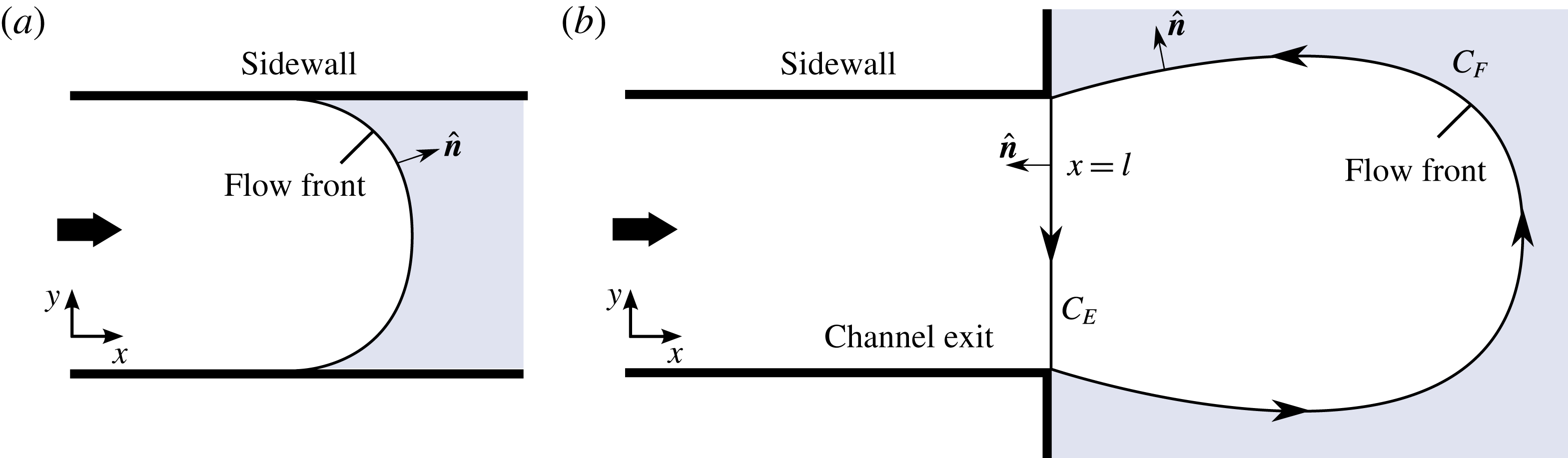
Plans of the situations where (a) the fluid front lies interior to the channel, and (b) the fluid front extends beyond the channel exit. In panel (b), the closed curve along which the line integral appearing in (2.16) is performed is indicated by arrows. The component representing the cross-section of the channel exit is denoted
 $C_{E}$
and that of the fluid front
 $C_{F}$
.

2.1 The dynamic condition at a flow front
Along the leading flow front of the current, illustrated in figure 2(a), I impose the stress condition
 $$\begin{eqnarray}\displaystyle \unicode[STIX]{x1D707}[(\unicode[STIX]{x1D735}\boldsymbol{\cdot }\boldsymbol{u})\hat{\boldsymbol{n}}+\unicode[STIX]{x1D65A}\boldsymbol{\cdot }\hat{\boldsymbol{n}}]={\textstyle \frac{1}{4}}\unicode[STIX]{x1D70C}g^{\prime }H\hat{\boldsymbol{n}}\quad \text{on }x=X(y,t), & & \displaystyle\end{eqnarray}$$
where
 $x=X(y,t)$
is the frontal position and
 $\hat{\boldsymbol{n}}$
is the unit horizontal normal along the leading edge (Pegler & Worster Reference Pegler and Worster2012). Note that a positive frontal thickness (
 $H>0$
) allows for the cliff-like terminus typical along the calving front of an ice shelf. Integrating the
 $x$
component of (2.13) across the width of the flow, using (2.9b
) to evaluate
 $\unicode[STIX]{x1D707}$
and rearranging, I obtain
 $$\begin{eqnarray}\frac{\unicode[STIX]{x2202}\bar{u}}{\unicode[STIX]{x2202}x}(X,t)=\left[\frac{\unicode[STIX]{x1D70C}g^{\prime }H(X,t)}{8\unicode[STIX]{x1D707}_{0}}\right]^{n},\end{eqnarray}$$
where the no-penetration condition (2.5b
) has been used to evaluate the boundary term involving
 $v$
. In obtaining (2.14), I have dropped the moduli in the viscosity (2.9b
) because the frontal rate of extension implied by (2.13) is always positive (
 $\unicode[STIX]{x2202}\bar{u}/\unicode[STIX]{x2202}x>0$
). Equation (2.14) represents a balance between the stress due to longitudinal extension and the discontinuity in depth-integrated hydrostatic pressure between the leading flow front and the ocean in front of it.
2.2 The dynamic condition at a channel exit
Once the layer extends beyond the exit of the channel (
 $X(t)>l$
), it forms a jet-like flow free of sidewall stresses, illustrated in figure 2(b) and later in the experimental photograph of figure 10. Assuming that the leading edge beyond the channel exit remains a free boundary (it does not contact a boundary downstream, say), the details of the flow downstream of the channel exit have no effect on the flow inside the channel and there is an effective boundary condition at the channel mouth that is independent of the flow beyond it. To develop this, I begin by rewriting (2.2) in the stress–divergence form
 $$\begin{eqnarray}\unicode[STIX]{x1D735}\boldsymbol{\cdot }\left(\unicode[STIX]{x1D707}H[(\unicode[STIX]{x1D735}\boldsymbol{\cdot }\boldsymbol{u})\unicode[STIX]{x1D644}+\unicode[STIX]{x1D65A}]-\frac{\unicode[STIX]{x1D70C}g^{\prime }}{4}H^{2}\unicode[STIX]{x1D644}\right)=0.\end{eqnarray}$$
With reference to figure 2(b), I perform an integral of (2.15) over the horizontal area bounded between the line
 $x=l$
, denoted by
 $C_{E}$
in figure 2(b), and the curve of the fluid front
 $C_{F}$
, to obtain, with use of the divergence theorem,
 $$\begin{eqnarray}\displaystyle & & \displaystyle \int _{C_{E}}\left\{\unicode[STIX]{x1D707}H[(\unicode[STIX]{x1D735}\boldsymbol{\cdot }\boldsymbol{u})\unicode[STIX]{x1D644}+\unicode[STIX]{x1D65A}]-\frac{\unicode[STIX]{x1D70C}g^{\prime }}{4}H^{2}\unicode[STIX]{x1D644}\right\}\boldsymbol{\cdot }(-\hat{\boldsymbol{x}})\,\,\text{d}s\nonumber\\ \displaystyle & & \displaystyle \quad +\int _{C_{F}}\underbrace{\left\{\unicode[STIX]{x1D707}H[(\unicode[STIX]{x1D735}\boldsymbol{\cdot }\boldsymbol{u})\unicode[STIX]{x1D644}+\unicode[STIX]{x1D65A}]-\frac{\unicode[STIX]{x1D70C}g^{\prime }}{4}H^{2}\unicode[STIX]{x1D644}\right\}}_{\mathbf{0}}\boldsymbol{\cdot }\,\hat{\boldsymbol{n}}\,\,\text{d}s=\mathbf{0},\end{eqnarray}$$
where
 $\hat{\boldsymbol{n}}$
is the unit horizontal normal to
 $C_{F}$
,
 $\hat{\boldsymbol{x}}$
is the unit vector in the
 $x$
direction and d
 $s$
is the line element. In accord with (2.13), the integral over the fluid front
 $\int _{C_{F}}$
is zero. With the same width integration and imposition of zero lateral velocity used to obtain (2.14) above, equation (2.16) similarly reduces to
 $$\begin{eqnarray}\frac{\unicode[STIX]{x2202}\bar{u}}{\unicode[STIX]{x2202}x}(l,t)=\left[\frac{\unicode[STIX]{x1D70C}g^{\prime }H(l,t)}{8\unicode[STIX]{x1D707}_{0}}\right]^{n}.\end{eqnarray}$$
The specification of zero lateral velocity
 $v$
near the corners of the channel exit may not in fact hold to good approximation if the flow undergoes a die swell in front of the channel exit. This point will be discussed in the context of my laboratory experiments in § 4.2.
In conclusion, the stress conditions at a fluid front (2.14) and at a channel exit (2.17) are equivalent. That is, the boundary condition at the mouth of a channel (2.17) is equivalent to fixing a fluid front at
 $x=l$
. The equivalence arises because the pressure of the ‘ocean’ communicates directly through the detached region of the layer to the channel exit. This is similar to the way that an idealized one-dimensional ice shelf transmits forces directly to the grounding line of a marine ice sheet (Weertman Reference Weertman1974). By allowing fluid to extend freely downstream of the sidewalls, it is thus possible to simulate the conditions that apply at a fixed calving front experimentally (see § 4).
2.3 Evolution of the thickness and fluid front
With
 $\bar{u}$
obtained from an integration of (2.12), the evolution of the thickness
 $H$
can be determined using the width-integrated form of the continuity equation (2.3),
 $$\begin{eqnarray}\frac{\unicode[STIX]{x2202}H}{\unicode[STIX]{x2202}t}+\frac{1}{s(x)}\frac{\unicode[STIX]{x2202}}{\unicode[STIX]{x2202}x}[s(x)H\bar{u}]=0,\end{eqnarray}$$
which is a one-dimensional advection equation. While not included here, the combined effects of snowfall accumulation and basal melting could be accommodated by including a distributed source (or sink) term of the form
 $a(x,t)$
on the right-hand side of (2.18). With the overdot used to denote
 $\text{d}/\text{d}t$
, I assume finally that the fluid front
 $X(t)$
evolves kinematically according to
 $$\begin{eqnarray}{\dot{X}}=\bar{u}(X,t).\end{eqnarray}$$
3 Transient dynamics and long-term steady flow
This section explores the introduction of a floating layer of viscous fluid into a channel of finite length. The fundamentals are considered first in the context of the simplest, Newtonian rheology (
 $n=1$
) and a channel of uniform width (
 $s^{\prime }\equiv 0$
). General power-law exponents
 $n$
will be considered in § 5.
To model the inflow, I impose conditions on the thickness and width-averaged velocity,
 $$\begin{eqnarray}\displaystyle H=d,\quad \bar{u}=Q/d\quad \text{at }x=0, & & \displaystyle\end{eqnarray}$$
respectively, where
 $d$
and
 $Q$
are the thickness and volumetric flux per unit width at which fluid is input, both assumed constant. The position of the source
 $x=0$
could be interpreted as the steady-state position of the grounding line of a marine ice sheet. By forming scaling relationships between the three force terms in (2.12) along with the scaling between thickness, velocity and flux implied by (3.1), namely
 $H\bar{u}\sim Q$
, I determine the scales of length, time, thickness and speed given by
 $$\begin{eqnarray}\displaystyle \mathscr{L}\equiv \left(\frac{s^{2}}{3}\right)^{1/2}\!,\quad \mathscr{T}\equiv \left(\frac{\unicode[STIX]{x1D707}\mathscr{L}}{\unicode[STIX]{x1D70C}g^{\prime }Q}\right)^{1/2}\!,\quad \mathscr{H}\equiv \left(\frac{\unicode[STIX]{x1D707}Q}{\unicode[STIX]{x1D70C}g^{\prime }\mathscr{L}}\right)^{1/2}\!,\quad \mathscr{U}\equiv \left(\frac{\unicode[STIX]{x1D70C}g^{\prime }Q\mathscr{L}}{\unicode[STIX]{x1D707}}\right)^{1/2}\!, & & \displaystyle \nonumber\\ \displaystyle & & \displaystyle\end{eqnarray}$$
respectively. These scales are intrinsic to regions of the flow where the forces due to extension, shear and buoyancy are all comparable. I define dimensionless variables by
 $$\begin{eqnarray}x\equiv \mathscr{L}\hat{x},\quad t\equiv \mathscr{T}\hat{t},\quad H\equiv \mathscr{H}{\hat{H}},\quad \bar{u}\equiv \mathscr{U}\hat{u} .\end{eqnarray}$$
With hats dropped, (2.12) and (2.18) become
 $$\begin{eqnarray}\displaystyle 4\displaystyle \frac{\unicode[STIX]{x2202}}{\unicode[STIX]{x2202}x}\left(H\displaystyle \frac{\unicode[STIX]{x2202}u}{\unicode[STIX]{x2202}x}\right)-Hu & = & \displaystyle H\displaystyle \frac{\unicode[STIX]{x2202}H}{\unicode[STIX]{x2202}x},\end{eqnarray}$$
 $$\begin{eqnarray}\displaystyle \displaystyle \frac{\unicode[STIX]{x2202}H}{\unicode[STIX]{x2202}t}+\displaystyle \frac{\unicode[STIX]{x2202}}{\unicode[STIX]{x2202}x}(Hu) & = & \displaystyle 0.\end{eqnarray}$$
The input conditions (3.1a,b ) become
 $$\begin{eqnarray}\displaystyle H(0,t)=D,\quad u(0,t)=D^{-1}. & & \displaystyle\end{eqnarray}$$
The frontal stress condition, given by (2.14) or (2.17), is
 $$\begin{eqnarray}\displaystyle \displaystyle \frac{\unicode[STIX]{x2202}u}{\unicode[STIX]{x2202}x}(X,t) & = & \displaystyle \frac{H}{8}\quad \text{if }X(t)\leqslant L\quad \text{(flow front),}\end{eqnarray}$$
 $$\begin{eqnarray}\displaystyle \displaystyle \frac{\unicode[STIX]{x2202}u}{\unicode[STIX]{x2202}x}(L,t) & = & \displaystyle \frac{H}{8}\quad \text{if }X(t)>L\quad \text{(channel exit).}\end{eqnarray}$$
 $$\begin{eqnarray}{\dot{X}}=u(X,t)\quad \text{if }X<L.\end{eqnarray}$$
The dimensionless model system above depends on two parameters,
 $$\begin{eqnarray}\displaystyle D\equiv \frac{d}{\mathscr{H}}\equiv \left(\frac{\unicode[STIX]{x1D70C}g^{\prime }\mathscr{L}}{\unicode[STIX]{x1D707}_{0}Q}\right)^{1/2}\!\!d,\quad L\equiv \frac{l}{\mathscr{L}}\equiv \sqrt{12}\frac{l}{w}, & & \displaystyle\end{eqnarray}$$
which represent the dimensionless input thickness and channel length, respectively. The parameter
 $D$
is the ratio of the input thickness
 $d$
to the thickness scale
 $\mathscr{H}$
. Its inverse
 $D^{-1}$
is the ratio of the width-averaged speed of input
 $Q/d$
to the speed scale
 $\mathscr{U}$
. The dimensionless channel length
 $L\approx 3.46\,(l/w)$
is a scaled horizontal aspect ratio. The case of unit aspect ratio,
 $l/w=1$
, characteristic of many ice shelves (see § 6), is represented by
 $L\approx 3.5$
.
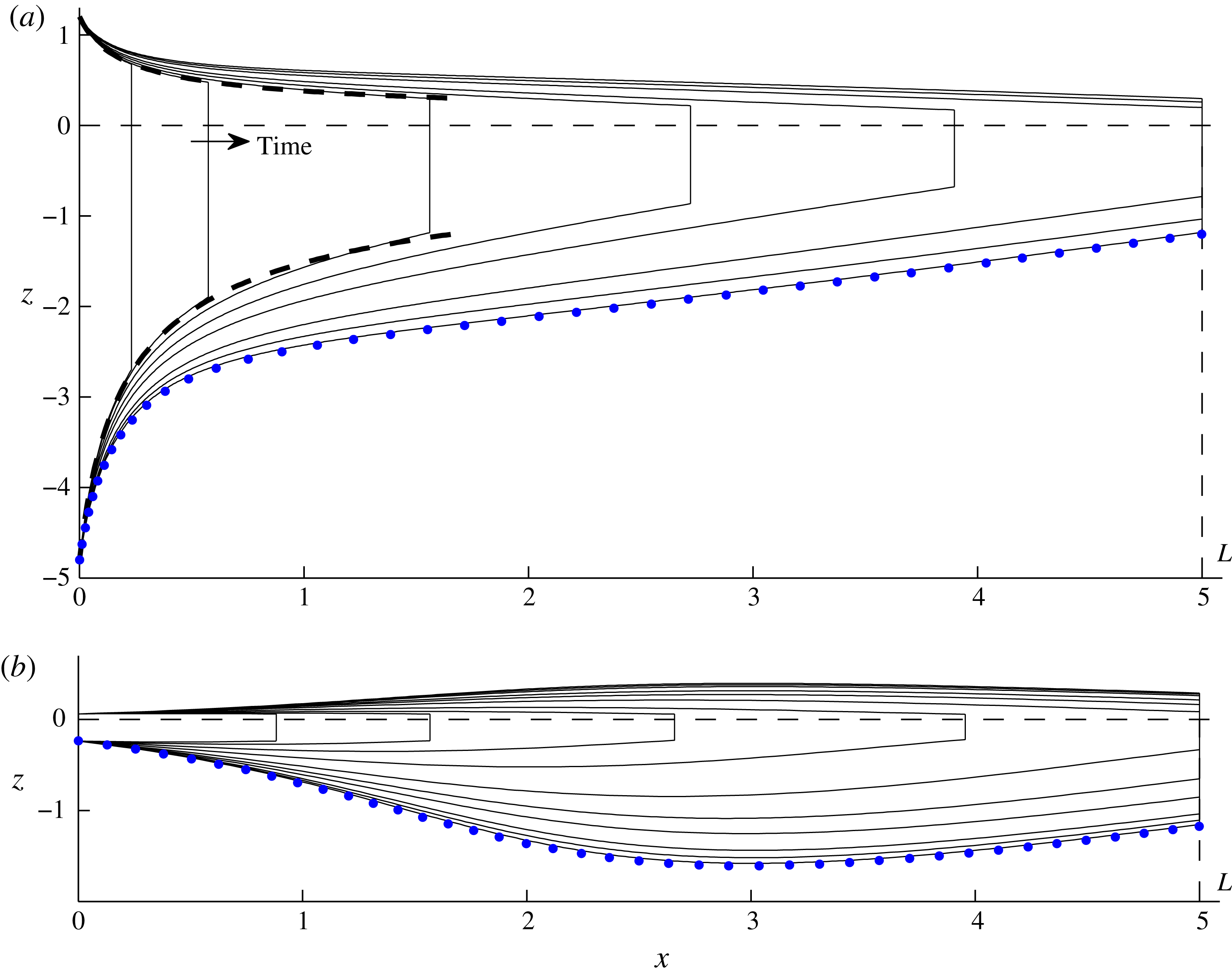
The numerically determined evolution of the surfaces of the layer at dimensionless times
 $t=1$
, 2, 4, 6, 8, 12, 16 and 32 for dimensionless channel length
 $L=5$
and dimensionless input thicknesses (a)
 $D=6$
and (b)
 $D=0.3$
. Two additional early times,
 $t=0.25$
and 0.5, are shown in panel (b). The envelopes describing the steady surfaces of the purely extensional regime (3.12) are shown by the dashed curves in panel (a), illustrating its occurrence as an early-time regime if
 $D\gtrsim 1$
. The late-time steady state (3.16) is shown by dotted blue curves in each case.

Two representative numerical solutions to (3.4)–(3.8) for (a)
 $D=6$
and (b)
 $D=0.3$
, each with
 $L=5$
, are shown in figures 3(a) and 3(b) respectively. These were obtained using a Lagrangian finite-difference scheme in which the flow domain
 $[0,X(t)]$
is discretized using time-dependent nodes that evolve with the flow (Pegler & Worster Reference Pegler and Worster2012). The scheme was initialized using the kinematic solution described in § 3.1 below.
With
 $D=6$
, the initial thinning of the fluid layer at early times is reminiscent of the steady, concave profile produced by a purely extensional one-dimensional flow. At late times, the flow approaches a steady state containing two dynamically distinct zones: a long region wherein the surfaces have relatively mild slope, and a shorter region near the input wherein the profile undergoes significant variation. For
 $D=0.3$
, the layer is introduced 20 times thinner but 20 times faster than when
 $D=6$
. The early-time flow is characteristically different. Instead of initially filling a near-steady concave profile, the flow undergoes a time-dependent thickening about its lengthways midpoint. At late times, the flows approach steady states. In these final states, the thicknesses and shapes of the profiles near the channel exit for these two cases of
 $D$
are almost identical. For example, the frontal thickness
 $H(L,t)$
differs by less than 0.1 %, despite the significant differences between the profiles further upstream.
3.1 Early-time flow and the intervention of sidewall stresses
As indicated by the second term in (2.12), transverse shear stresses are larger for smaller channel widths
 $w=2s$
. It is therefore reasonable to expect shear stresses to be negligible if the length of the flow is much shorter than the width (
 $w=2s\gg X(t)\mathscr{L}$
), as applies at sufficiently early times. In the absence of the shear-stress term
 $Hu$
, equation (3.4) reduces to
 $$\begin{eqnarray}4\frac{\unicode[STIX]{x2202}}{\unicode[STIX]{x2202}x}\left(H\frac{\unicode[STIX]{x2202}u}{\unicode[STIX]{x2202}x}\right)=H\frac{\unicode[STIX]{x2202}H}{\unicode[STIX]{x2202}x},\end{eqnarray}$$
which is equivalent to the one-dimensional form of (2.2). A direct first integral of this equation subject to (3.7a ) yields
 $$\begin{eqnarray}\frac{\unicode[STIX]{x2202}u}{\unicode[STIX]{x2202}x}=\frac{1}{8}H,\end{eqnarray}$$
which implies that, with no sidewall stresses, the rate of horizontal extension is everywhere proportional to the thickness (not only at the front, as implied by (3.7a )). With reference to (3.4), this direct integration cannot be performed with sidewall stresses, as they form a component of the divergence of deviatoric stresses that is distinct from the gradient in pressure (an analogous situation occurs with viscous hoop stresses (see Pegler & Worster Reference Pegler and Worster2012)). Combining (3.5), (3.6) and (3.11), one can determine the analytical solution
 $$\begin{eqnarray}\displaystyle H & = & \displaystyle (D^{-2}+{\textstyle \frac{1}{4}}x)^{-1/2}\quad \text{in }0\leqslant x\leqslant X(t),\end{eqnarray}$$
 $$\begin{eqnarray}\displaystyle X(t) & = & \displaystyle D^{-1}t+{\textstyle \frac{1}{16}}t^{2}\equiv X_{E}(t)\end{eqnarray}$$
 $D=6$
. The numerical solution begins to deviate from the envelope significantly by
 $t\approx 4$
as sidewall stresses intervene.
In order to explore when deviation from the purely extensional regime (3.12) occurs across the full range of
 $D$
, I calculate the time
 $t_{E}$
defined by
 $$\begin{eqnarray}X(t_{E})=0.98X_{E}(t_{E}),\end{eqnarray}$$
which represents when the frontal position
 $X$
first deviates from the position
 $X_{E}$
implied by (3.12b
) by 2 %. As shown in figure 4,
 $t_{E}$
increases with
 $D$
, implying that a larger input thickness favours the endurance of the extensional regime. However,
 $t_{E}\rightarrow 3.6$
remains finite as
 $D\rightarrow \infty$
, implying that, even when conditions ideally favour the endurance of the extensional regime, sidewall stresses intervene significantly by
 $t=3.6$
. At this time, the dimensional length is comparable to just one-quarter of a channel width (
 $X\mathscr{L}\approx 0.24w$
).
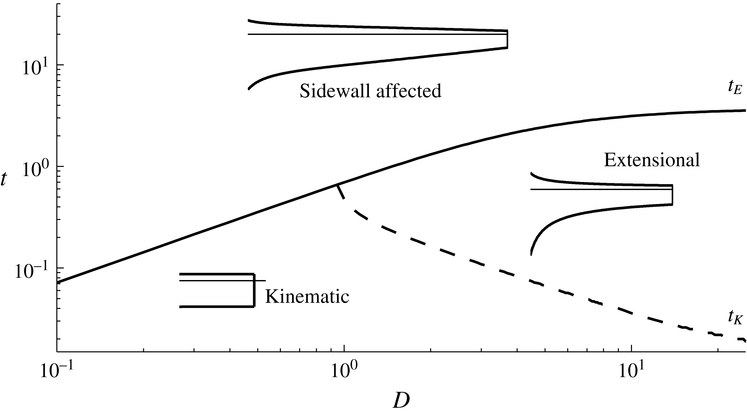
Parameter–time regime diagram showing when the two possible early-time flow regimes of kinematic and extensional flow occur as a function of the dimensionless input thickness
 $D$
. Before the time
 $t_{E}$
, defined by (3.13) and shown by a solid curve, the flow is described to good approximation by the purely extensional flow regime (3.12). For
 $t>t_{E}$
, the flow has been influenced significantly by sidewall stresses. The earlier time
 $t_{K}$
defined by
 $X(t_{K})=1.02D^{-1}t$
represents the time up to which the flow is controlled kinematically by the input speed (3.6b
). Sidewall stresses always intervene significantly by
 $t\approx 3.6$
, even when conditions are optimized for the endurance of the extensional regime.

There is a further transition time
 $t_{K}$
, which I define by
 $X(t_{K})=1.02D^{-1}t_{K}$
, up to which the flow is simply controlled kinematically by the input flow speed (3.6b
). The time
 $t_{K}$
is shown by a dashed curve in figure 4. For
 $D>1$
, the buoyancy-driven contribution to (3.12b
), represented by the quadratic term
 $t^{2}/16$
, is only significant in the interval
 $t_{K}<t<t_{E}$
. For
 $D<1$
, this interval does not exist, implying that sidewall stresses intervene before buoyancy forces in these cases. The concave regime of (3.12) then never occurs, as evidenced by the example with
 $D=0.3$
in figure 3(b). In conclusion, the one-dimensional regime (3.12) breaks down over all parameter settings once lateral contact exceeds one-quarter of a flow width.
3.2 Steady state
At late times, the flows approach steady states, shown by blue dotted curves in figure 3(a,b). Using the steady form of (3.5) (
 $Hu=1$
) to eliminate
 $u$
in the second term of (3.4), I obtain the ordinary differential equation
 $$\begin{eqnarray}4\frac{\text{d}}{\text{d}x}\left(H\frac{\text{d}u}{\text{d}x}\right)-1=\frac{\text{d}}{\text{d}x}\left(\frac{H^{2}}{2}\right),\end{eqnarray}$$
where the dimensionless transverse shear stress, represented by the
 $-1$
on the left-hand side, is (favourably) uniform. Integration of (3.14) subject to (3.7b
) yields
 $$\begin{eqnarray}4H\frac{\unicode[STIX]{x2202}u}{\unicode[STIX]{x2202}x}=\underbrace{\frac{1}{2}H^{2}}_{\text{buoyancy}}\;\underbrace{-\,(L-x)}_{\text{lateral stress}},\end{eqnarray}$$
which generalizes (3.11) to accommodate lateral stresses. This equation shows that the effect of lateral stress is to reduce the rate of extension in proportion to the distance from the channel mouth
 $(L-x)$
. In physical terms, the equation shows that the normal stress associated with driving fluid forwards through the channel (or back-force) at any point, represented by the left-hand side, is proportional to the distance downstream over which the flow contacts the sidewalls. Lateral stresses have no effect on the force balance at the channel mouth,
 $x=L$
, where the dominant balance is between buoyancy and extension alone in accord with (3.7b
).
Using the mass conservation equation
 $u=1/H$
to eliminate
 $u$
fully in (3.15), I integrate (3.15) further subject to the input condition (3.6a
) to obtain the exact analytical solution
 $$\begin{eqnarray}H^{-2}=\text{e}^{(L-x)^{2}/4}\left(D^{-2}\text{e}^{-L^{2}/4}+\frac{1}{2}\int _{(L-x)/2}^{L/2}\text{e}^{-\unicode[STIX]{x1D709}^{2}}\,\,\text{d}\unicode[STIX]{x1D709}\right),\end{eqnarray}$$
which produces the blue dotted curves in figure 3. A suite of the steady solutions (3.16) is plotted in figure 5 for (a) a fixed input thickness
 $D=6$
and various flow lengths
 $L=1{-}5$
, and (b) a fixed flow length
 $L=5$
and various input thicknesses
 $D=0.2{-}\infty$
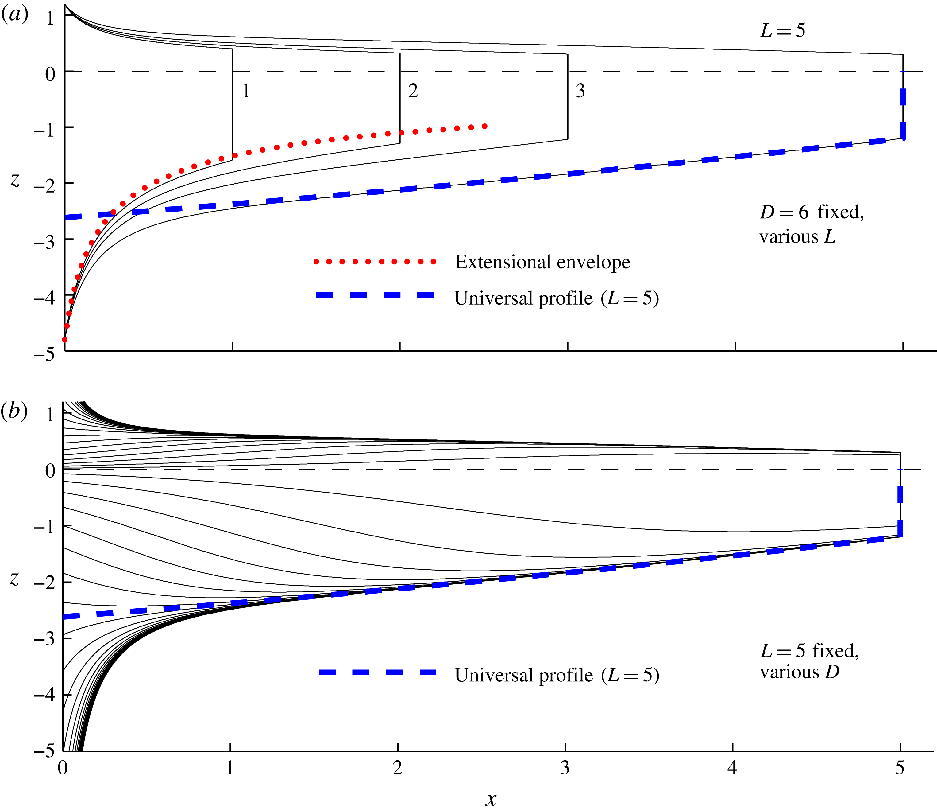
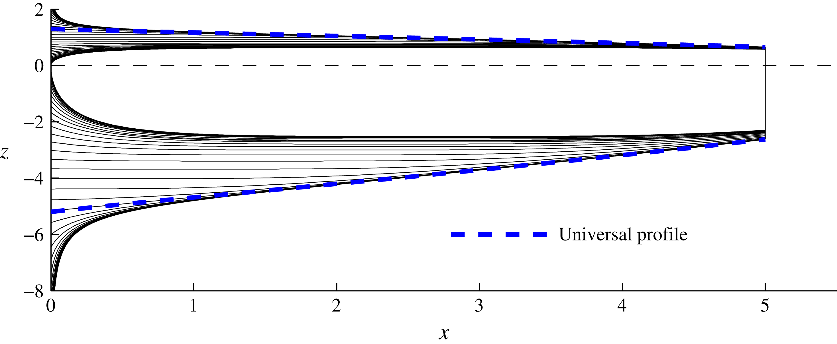
. Figure 5(a) illustrates the emergence of two characteristically different steady-state flow regimes, depending on whether the flow is sufficiently short or long.
(a) The steady-state surface profiles predicted by (3.16) for various flow lengths
 $L=1{-}5$
and a fixed input thickness
 $D=6$
. The two possible flow regimes that occur depending on the flow length
 $L$
are illustrated. In the short case
 $L=1$
, the flow can be treated as effectively one-dimensional and approximated well by the envelope (3.17), which is shown for the lower surface by a red dotted curve. In the longer case
 $L=5$
, the prevailing flow is instead described by the universal profile (3.18) shown by a dashed blue curve for
 $L=5$
. (b) A suite of solutions for a range of input thicknesses
 $D=0.2{-}\infty$
and fixed length
 $L=5$
, illustrating their spatial adjustment from the input towards the universal profile (3.18).

For a sufficiently short length
 $L$
, equation (3.16) recovers the one-dimensional steady-state profile of (3.12a
) asymptotically. This is demonstrated by taking the limit
 $L\rightarrow 0$
in (3.16), for which the exponentials can all be approximated as unity to leading order and (3.16) reduces asymptotically to
 $$\begin{eqnarray}H\sim (D^{-2}+{\textstyle \frac{1}{4}}x)^{-1/2},\end{eqnarray}$$
which is indeed equivalent to (3.12a
). The asymptotic extensional envelope (3.17) is shown as a red dotted curve in figure 5(a) and is confirmed to describe the short steady-state solutions with
 $L=1$
and 2 to good approximation.
For sufficiently large
 $L$
, equation (3.17) fails to provide a good approximation. Instead, a new regime arises, characterized by a rapid spatial adjustment from the input towards a prevailing region of relatively milder slope. The flow in this downstream region is of a universal dimensionless form up to translation with respect to the exit of the channel. Its universality is demonstrated in figure 5(b), where steady states over a large range of input thickness
 $D$
are shown to approach a single profile shown by the blue dashed curve. The universality is also consistent with the earlier observation in figure 3 that the steady-state frontal thicknesses in the two cases
 $D=6$
and 0.3 are effectively equal.
3.3 Universal downstream profile
By considering the limit
 $L\rightarrow \infty$
with
 $x\leqslant L$
, equation (3.16) reduces asymptotically to
 $$\begin{eqnarray}\displaystyle H^{-2}\sim H_{\ast }(x)^{-2} & \equiv & \displaystyle \frac{1}{2}\text{e}^{(L-x)^{2}/4}\int _{(L-x)/2}^{\infty }\text{e}^{-\unicode[STIX]{x1D709}^{2}}\,\,\text{d}\unicode[STIX]{x1D709}\nonumber\\ \displaystyle & \equiv & \displaystyle \frac{1}{4}\sqrt{\unicode[STIX]{x03C0}}\,\text{erfcx}\,\!\left[\frac{1}{2}(L-x)\right],\end{eqnarray}$$
where
 $\text{erfcx}\,\unicode[STIX]{x1D701}\equiv \text{e}^{\unicode[STIX]{x1D701}^{2}}(1-\text{erf}\,\unicode[STIX]{x1D701})$
is the scaled complementary error function. This expression represents the universal profile towards which the steady states adjust spatially, shown by the blue dashed curve in figure 5 for
 $L=5$
. The universal profile (3.18) varies only with distance backwards from the front
 $(L-x)$
. Therefore, with respect to the front,
 $x=L$
, it is of a universal dimensionless form. In particular, the thickness and flow rate at the front itself take the special values
 $$\begin{eqnarray}\displaystyle H_{c} & \equiv & \displaystyle H_{\ast }(L)=2\unicode[STIX]{x03C0}^{-1/4}\approx 1.502,\end{eqnarray}$$
 $$\begin{eqnarray}\displaystyle u_{c} & \equiv & \displaystyle u_{\ast }(L)=1/H_{\ast }(L)\approx 0.666,\end{eqnarray}$$
 $L$
, which predicts that
 $H(L)=(D^{-1}+L/4)^{-1/2}$
. By contrast, the predictions of (3.19) are entirely independent of
 $D$
and
 $L$
. These differences imply a fundamental alteration in the way that the flow structure of an ice shelf is determined between short and long flow lengths. For a short length, the profile (3.17) is determined causally from the input conditions, with no dependence on downstream conditions. It is sensitive in particular to the specific thickness imposed at the input
 $D$
. For long lengths, there is a reversal in the manner in which the profile is determined. Conditions at the downstream front (3.19) set the reference conditions from which the prevailing flow is determined. This flow is of a universal dimensionless form (up to scaling by (3.2)) that, in contrast to the purely extensional limiting form (3.17), is independent of the specified input thickness
 $D$
and depends only on the position of the downstream channel exit
 $L$
.
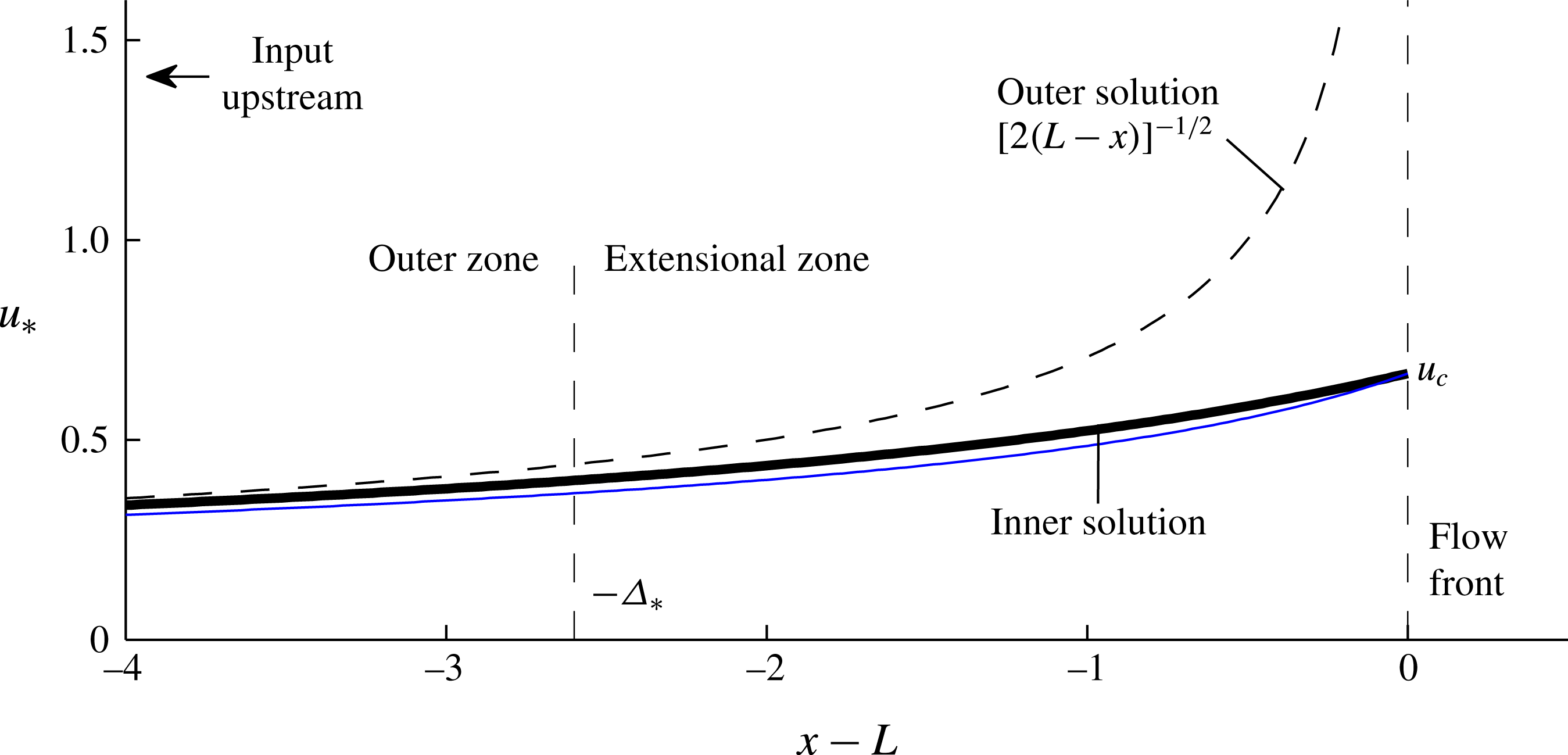
The along-channel velocity profile
 $u_{\ast }=1/H_{\ast }$
of the universal downstream profile (3.18) (solid black curve). The plot illustrates its boundary-layer structure comprising an outer zone of transverse-shear-dominated flow described to leading order by (3.20b
) (dashed black curve), and the inner ‘extensional zone’ wherein the extensional stress at the flow front (3.7b
) has a significant effect and is responsible for regularizing the flow speed. The extensional zone has a characteristic length
 $\unicode[STIX]{x1D6E5}_{\ast }\approx 2.6$
. The analytical approximation to the velocity of the universal profile based on neglecting only the divergence of extensional stresses, given by
 $u_{\ast }=1/H_{\ast }$
, with
 $H_{\ast }$
approximated by (3.21), is shown by the solid blue curve.

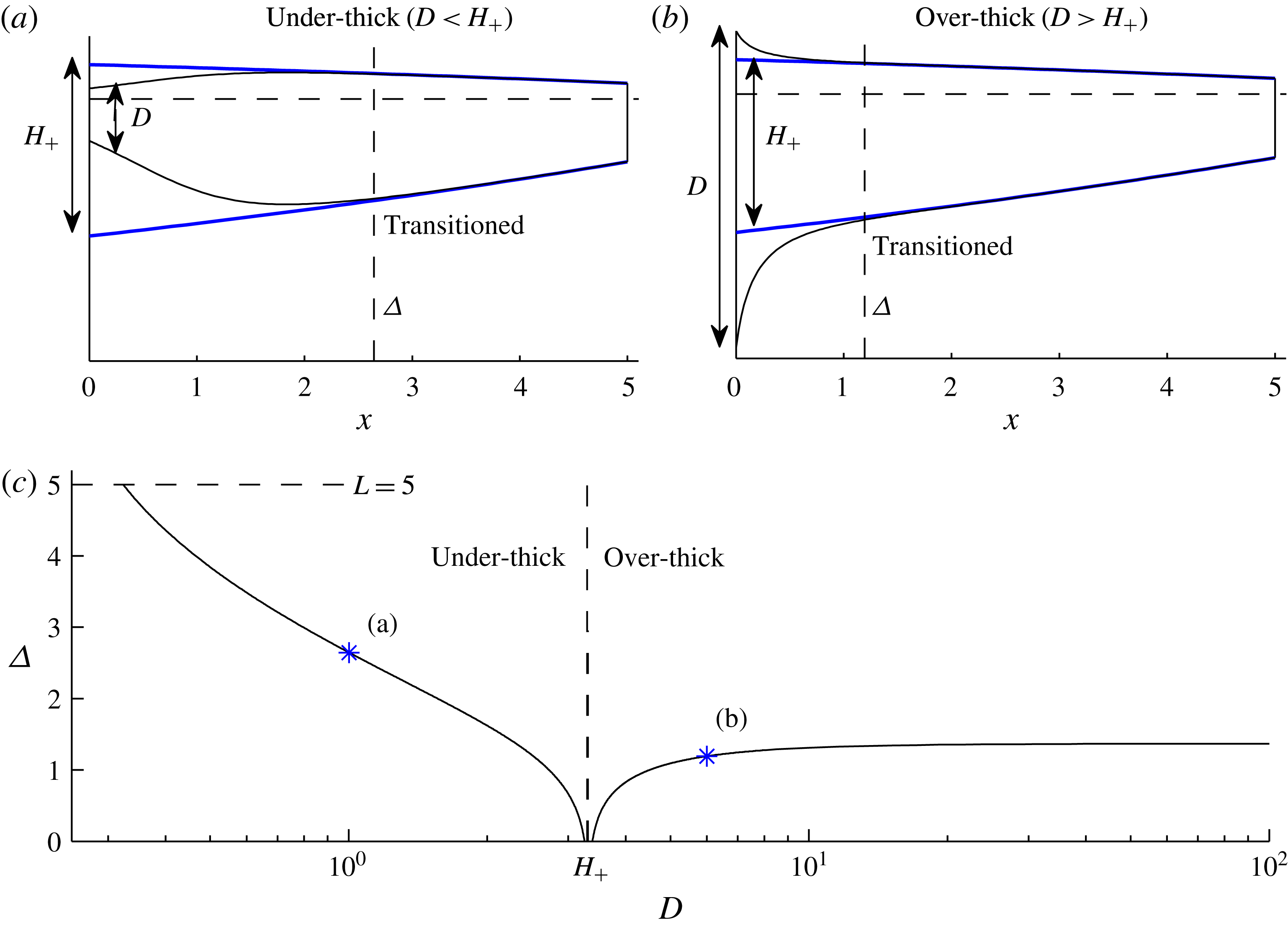
(a) An under-thick input thickness
 $D=1<H_{+}$
and (b) an over-thick input thickness
 $D=6>H_{+}$
, each for
 $L=5$
, where
 $H_{+}\approx 3.75$
is defined as the value of the universal profile (blue) extrapolated to the input (3.22). The transition length
 $\unicode[STIX]{x1D6E5}$
defined by (3.24) for
 $\unicode[STIX]{x1D716}=0.02$
is shown by a vertical dashed line in each case. (c) Plot of
 $\unicode[STIX]{x1D6E5}$
as a function of
 $D$
for
 $L=5$
, illustrating its increase with
 $|D-H_{+}|$
and maximal value of 1.4 for over-thick inputs.

3.3.1 Boundary-layer structure
Far upstream of the channel exit (
 $L-x\gg 1$
), the solution for the universal profile (3.18) predicts that the thickness grows significantly larger than the frontal thickness,
 $H\gg H_{c}$
. If the input lies sufficiently far upstream, there is a region in which the thickness predicted by (3.18), and its associated velocity
 $u_{\ast }=1/H_{\ast }$
, reduce asymptotically to
 $$\begin{eqnarray}\displaystyle H_{\ast }\sim [2(L-x)]^{1/2},\quad u_{\ast }\sim [2(L-x)]^{-1/2}\quad \text{for }L-x\gg 1, & & \displaystyle\end{eqnarray}$$
which are obtained on substitution of the large-
 $\unicode[STIX]{x1D701}$
asymptote
 $\text{erfcx}\,\unicode[STIX]{x1D701}\sim (\sqrt{\unicode[STIX]{x03C0}}\unicode[STIX]{x1D701})^{-1}$
in (3.18). Expression (3.20) represents the steady state that would arise under an assumption of uniformly transverse-shear-dominated flow, considered in a time-dependent context by Pegler et al. (Reference Pegler, Kowal, Hasenclever and Worster2013). This is confirmed by noting that the expression (3.20a
) is also obtained by integrating (3.14) with the first, extensional term neglected and solved subject to the zero-stress form of condition (3.7b
), namely,
 $H\rightarrow 0$
as
 $x\rightarrow L$
.
As shown in figure 6, equation (3.20) matches (3.18) to good approximation for
 $x\lesssim L-3$
and deviates from it significantly near the channel exit. At the exit itself,
 $x=L$
, the speed predicted by (3.20b
) is infinite, contrasting with the finite frontal speed predicted by the exact expression (3.19b
). This mismatch reflects a significant breakdown of the assumption of negligible extensional stresses underlying (3.20). More specifically, there is a boundary-layer structure comprising an outer region of lateral-drag-dominated flow described to leading order by (3.20) connected to an inner ‘extensional zone’ near the flow front wherein extensional stresses regularize the velocity field to meet condition (3.7b
). This structure is consistent with that suggested by Hindmarsh (Reference Hindmarsh2012) and qualitatively similar to the transition from a basal-drag-dominated grounded ice sheet to an extension-dominated ice shelf (Schoof Reference Schoof2007). The universal profile (3.18) differs from its outer region (3.20) by more than 10 % in a region of length
 $\unicode[STIX]{x1D6E5}_{\ast }\approx 2.6$
, implying a characteristic length for the extensional zone of three-quarters of a flow width (
 $\unicode[STIX]{x1D6E5}_{\ast }\mathscr{L}=0.75w$
).
The reduction of the universal profile to (3.20) is based on assuming that two distinct contributions involving extensional stresses are small: one is the left-hand side of (3.7b ); the other is the divergence of extensional stresses represented by the first term in (3.4) or (3.14). Strictly, both are of order unity in the extensional zone but, remarkably, the deviation between (3.18) and (3.20) is almost exclusively caused by the frontal extensional stress (3.7b ): the first, extensional term in (3.14) is effectively negligible. To show this, I integrate (3.14) with just the first term neglected to yield
 $$\begin{eqnarray}H_{\ast }\approx [H_{c}^{2}+2(L-x)]^{1/2},\end{eqnarray}$$
where
 $H_{c}$
is a constant of integration representing the thickness at the flow front. As illustrated by the blue curve in figure 6, the approximation (3.21) is numerically very close to the exact result (3.18), with the largest relative difference of 8 % occurring at
 $x\approx L-2$
. The numerical similarity confirms that the divergence of extensional stresses in (3.14) can be effectively neglected. The ability to neglect this term to good approximation presents a useful analytical tool, which I use in § 5 to obtain near-exact analytical solutions in cases of power-law fluid for which exact solutions like (3.18) are unavailable.
3.4 The input transition zone
As one follows the universal profile (3.18) upstream, its thickness
 $H_{\ast }(x)$
will generally conflict with the thickness imposed at the input,
 $H_{\ast }(0)\neq D$
. This conflict is resolved within a short transition zone involving significant extensional stresses, wherein conditions at the input are matched to the universal profile (3.18).
As an indication of the degree of conflict between the input conditions and the universal profile, I compare
 $D$
to the thickness of the profile (3.18) extrapolated to the input, namely,
 $$\begin{eqnarray}H_{+}(L)\equiv H_{\ast }(0)=2\unicode[STIX]{x03C0}^{-1/4}\left[\text{erfcx}\,\left({\textstyle \frac{1}{2}}L\right)\right]^{-1/2}.\end{eqnarray}$$
If
 $D>H_{+}$
, the flow is called over-thick and characterized by a spatial adjustment to the universal profile involving thinning and accelerated flow, as illustrated in figure 7(b). If
 $D<H_{+}$
, the flow is under-thick, as illustrated in figure 7(a).
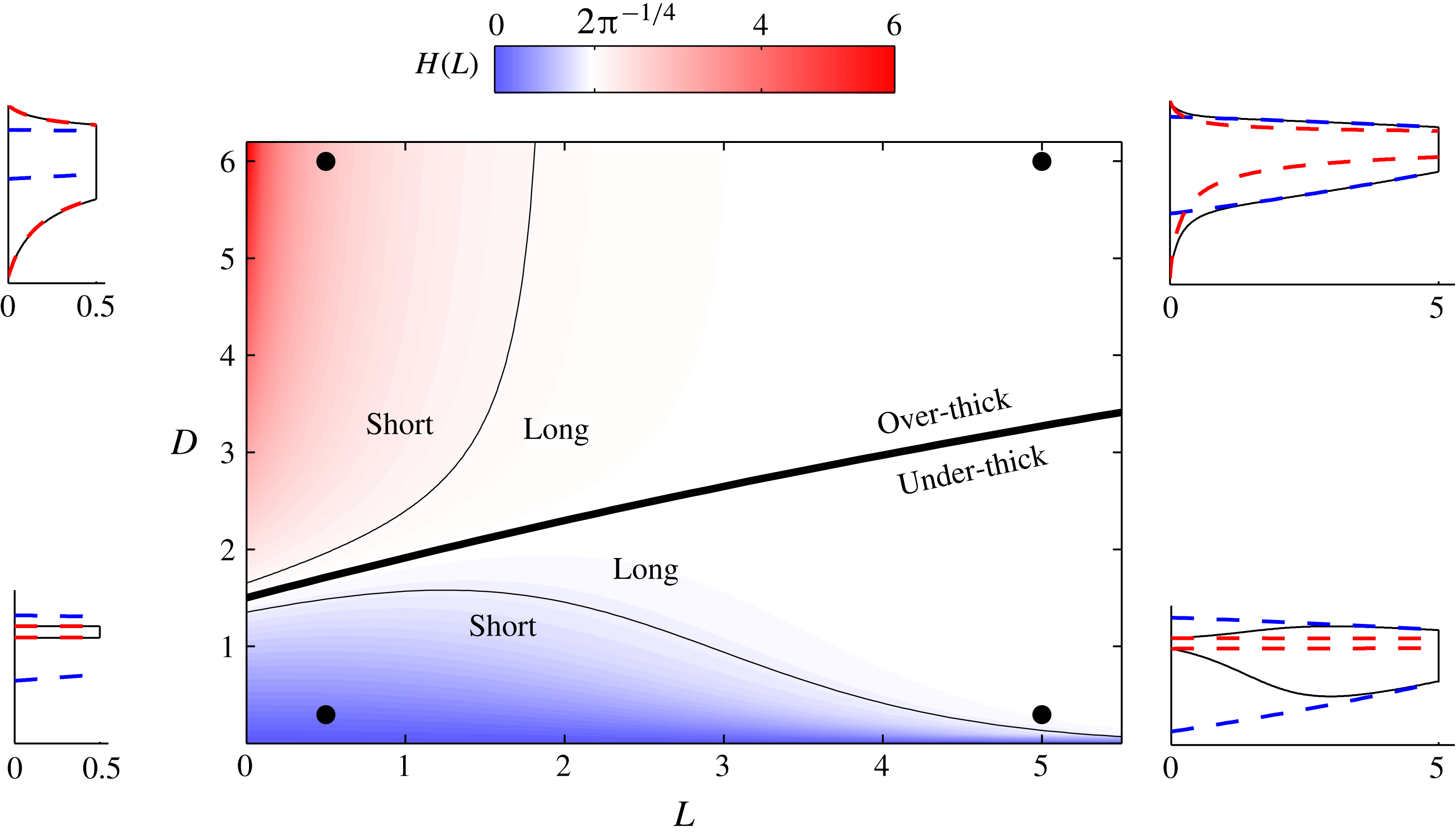
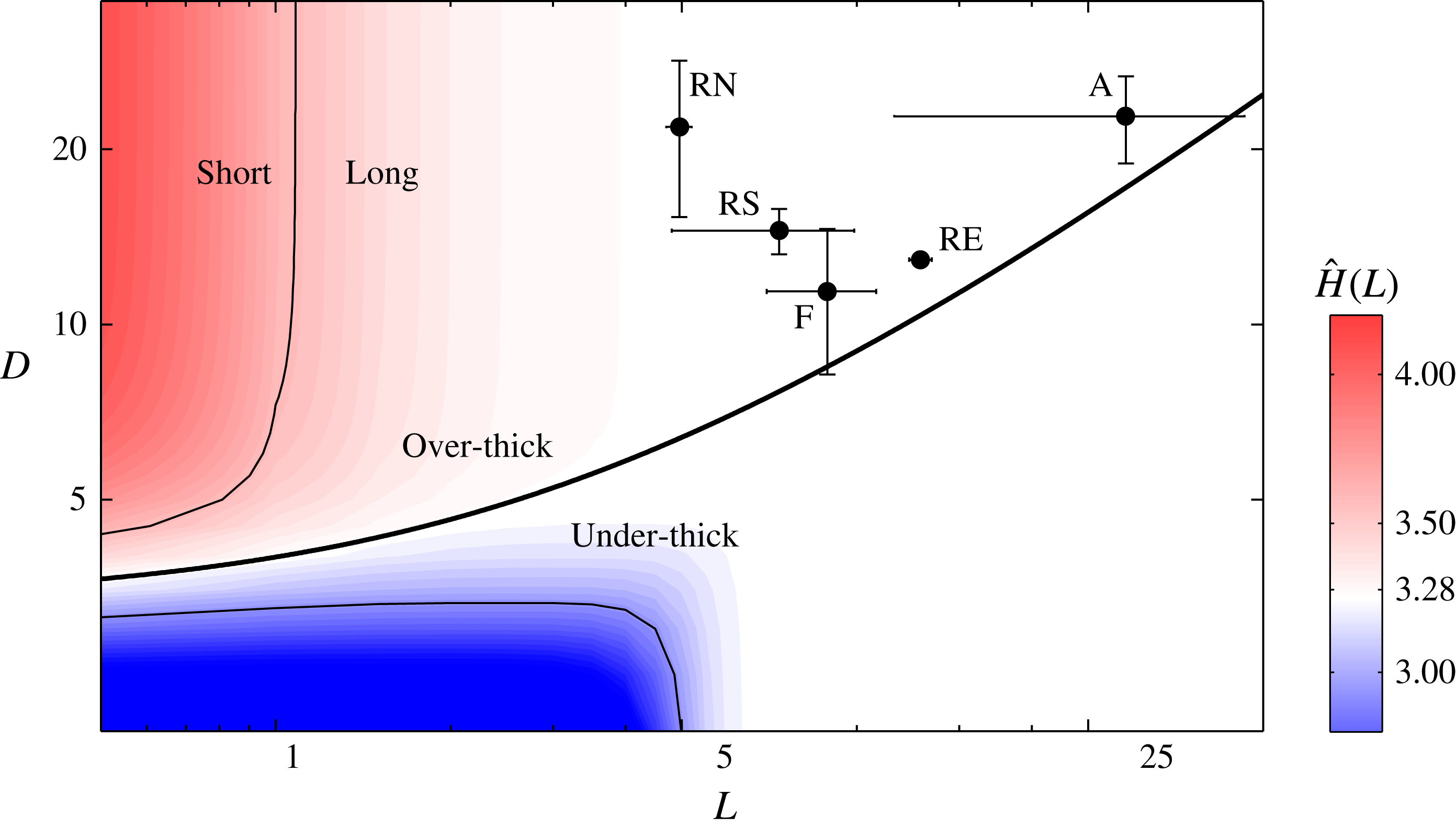
Regime diagram for steady states over the full parameter space
 $(L,D)$
. Colour indicates the dimensionless thickness at the flow front,
 $H(L)$
. White represents the special value associated with the universal profile (3.19a
),
 $H_{c}=2\unicode[STIX]{x03C0}^{-1/4}\approx 1.50$
. White regions indicate regimes for which a transition towards the universal profile completes fully. Red represents an ‘over-thick’ case defined by a frontal thickness greater than the special value,
 $H(L)>H_{c}$
, and blue represents an ‘under-thick’ case defined by
 $H(L)<H_{c}$
. The critical line separating the two is shown by a thick curve. The off-white regions (blue and red) indicate ‘short’ flows for which the adjustment towards the universal profile is incomplete. The contours
 $H(L)=(1\pm 0.1)H_{c}$
represent the boundary between ‘short’ and ‘long’. Insets illustrate the side-view profiles for the four parameter settings at the black circles, with the downstream universal profile (3.18) shown by the blue dashed curves in each inset and the purely extensional solution (3.12) by the red dashed curves.

The transition zone at the input can be interpreted as a boundary layer in which the information associated with the input thickness
 $D$
is dissipated and the flow transitions to the outer region represented by the universal profile (3.18) (this boundary-layer structure is distinct from that of the universal profile itself discussed in § 3.3.1). In the limit
 $L\rightarrow \infty$
, equation (3.18) reduces asymptotically to
 $$\begin{eqnarray}\displaystyle H^{-2}\sim [2(L-x)]^{-1}+(D^{-2}-H_{+}^{-2})\text{e}^{-Lx/2}, & & \displaystyle\end{eqnarray}$$
where
 $H_{+}^{2}\sim 2L$
, which describes the transition zone as a perturbation from the outer solution of the universal profile (3.20a
). The perturbation, represented by the second term, decays exponentially over a distance proportional to the dimensionless length scale
 $2L^{-1}$
and, as expected, increases with the absolute difference between
 $D$
and
 $H_{+}$
.
To determine more precisely the size of the input transition zone, I define the transition length
 $\unicode[STIX]{x1D6E5}=\unicode[STIX]{x1D6E5}(L,D)$
as the position
 $x=\unicode[STIX]{x1D6E5}$
at which
 $$\begin{eqnarray}H(\unicode[STIX]{x1D6E5})=(1\pm \unicode[STIX]{x1D716})H_{\ast }(\unicode[STIX]{x1D6E5}),\end{eqnarray}$$
where
 $\unicode[STIX]{x1D716}$
is a small parameter taken as 0.02. The position
 $x=\unicode[STIX]{x1D6E5}$
is indicated by a vertical dashed line in figure 7(a,b) and plotted as a function of
 $D$
in figure 7(c). The plot confirms that
 $\unicode[STIX]{x1D6E5}$
increases with the difference between
 $D$
and
 $H_{+}$
. If
 $D\approx H_{+}$
, there is no appreciable transition zone,
 $\unicode[STIX]{x1D6E5}\approx 0$
, and the whole flow is described uniformly by the universal profile (3.18). As
 $D\rightarrow \infty$
,
 $\unicode[STIX]{x1D6E5}\rightarrow 1.4$
remains finite, implying that any over-thick input,
 $D>H_{+}$
, results in a transition to the universal profile within half a channel width (
 $1.4\mathscr{L}\approx 0.40w$
). The transition length can become larger in under-thick cases
 $D<H_{+}$
. Indeed, for
 $D<0.3$
the (hypothetical) transition length exceeds the flow length
 $\unicode[STIX]{x1D6E5}>L=5$
and the transition to the universal profile remains incomplete. The dependences of
 $\unicode[STIX]{x1D6E5}$
on
 $D$
and
 $H_{+}(L)$
are encapsulated by the analytical approximation
 $$\begin{eqnarray}\unicode[STIX]{x1D6E5}\approx \frac{4}{H_{+}^{2}}\ln \left|\frac{D^{2}-H_{+}^{2}}{2\unicode[STIX]{x1D716}D^{2}}\right|,\end{eqnarray}$$
obtained by using (3.20a
) and (3.23) to evaluate
 $H_{\ast }$
and
 $H$
in (3.24), respectively. The result (3.25) implies that
 $\unicode[STIX]{x1D6E5}\rightarrow 4H_{+}^{-2}\ln (1/2\unicode[STIX]{x1D716})$
as
 $D\rightarrow \infty$
, which confirms that
 $\unicode[STIX]{x1D6E5}$
remains finite in this limit. This asymptotic prediction is within 6 % of the numerically determined value. The outlying multiplicative factor
 $\propto H_{+}^{-2}$
in (3.25) implies that a larger matching thickness
 $H_{+}$
(a thicker downstream flow) results in a shorter transition length
 $\unicode[STIX]{x1D6E5}$
. This is because a thicker downstream flow exerts a larger back-force, which resists flow in the input transition zone and causes the transition to take place over a shorter distance.
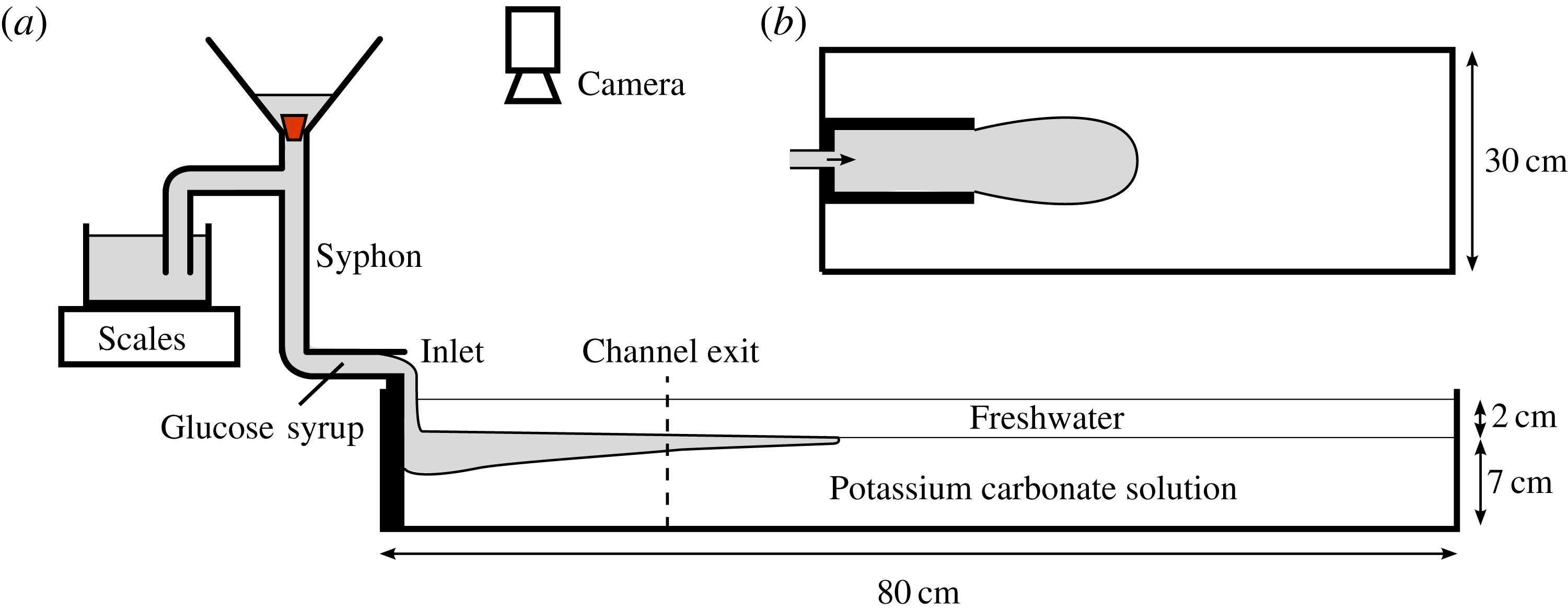
(a) Horizontal cross-section and (b) plan view of my experimental set-up.

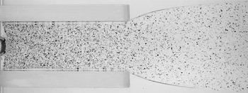
Plan-view photograph of a fully developed experiment showing the floating film of particle-laden syrup fed from the left and propagating to the right between sidewalls of length 16 cm and width 6 cm. The die swell beyond the channel exit is illustrated.

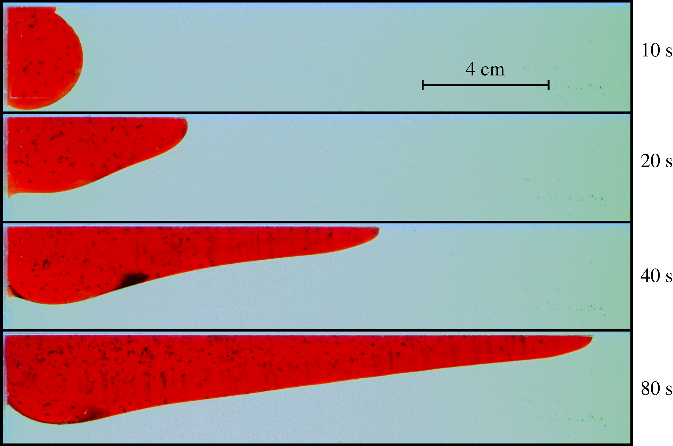
Sequence of side-view photographs of an experiment at times
 $t=10$
, 20, 40 and 80 s after the initialization of the input, illustrating the development of the fluid layer and its under-thick input transition. The upper layer of water used to reduce the effects of surface tension in my other experiments was not included in this purely illustrative experiment in order to avoid optical distortion.

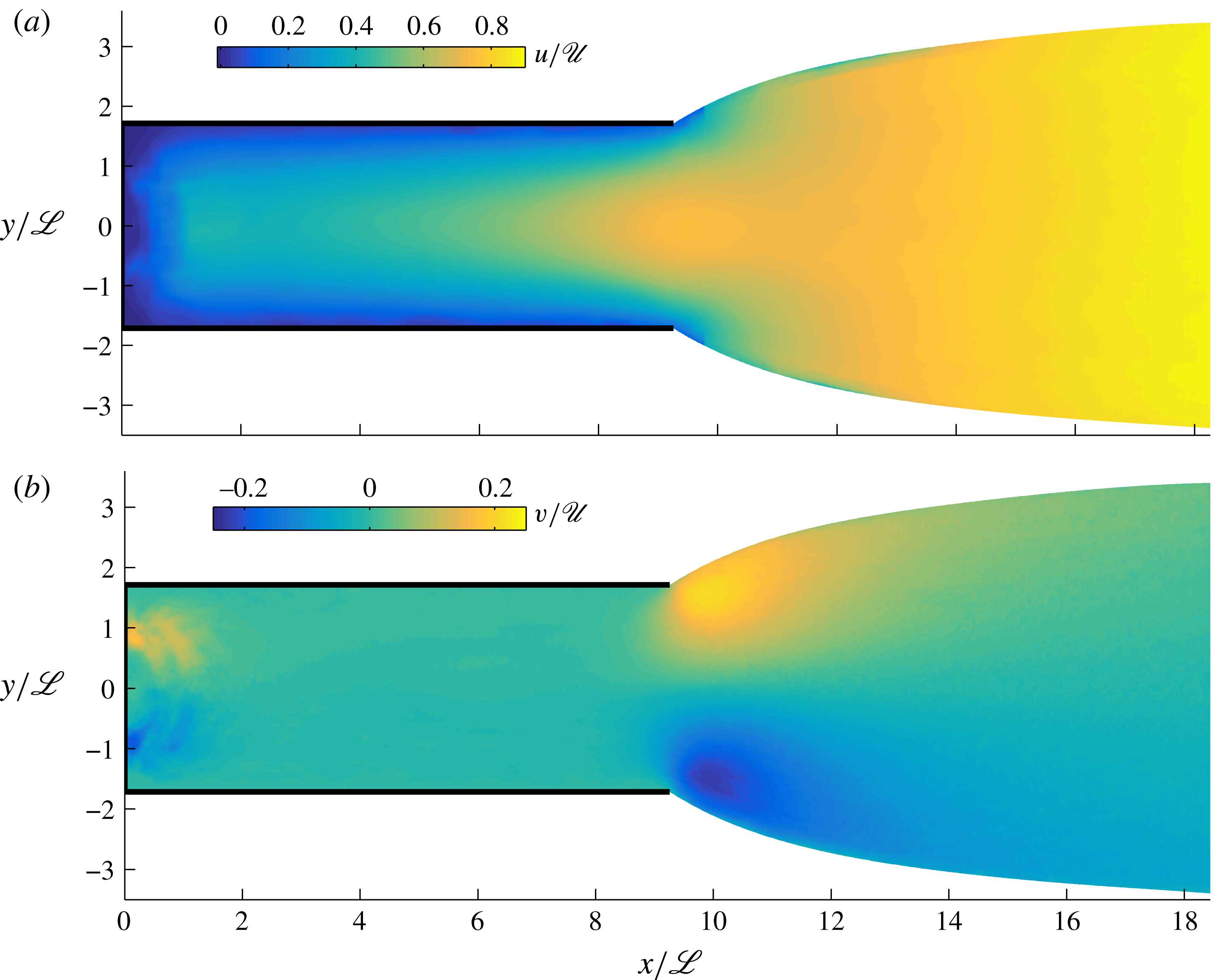
Experimental data for the (plan-view) two-dimensional velocity field obtained using PIV on the late-time steady flow of experiment B. (a) The dimensionless longitudinal velocity
 $u/\mathscr{U}$
and (b) the transverse velocity
 $v/\mathscr{U}$
, plotted in the dimensionless coordinate system
 $(x/\mathscr{L},y/\mathscr{L})$
. The data show a transition from a qualitatively parabolic shear flow with negligible transverse velocity inside the channel to a plug-like extensional flow beyond the channel exit. Significant transverse velocities at the corners of the channel mouth drive a die swell beyond the channel mouth.

3.5 Regime classification
The results above show that a transition towards the universal profile completes for all
 $D>0.3$
if
 $L=5$
. With the shorter length
 $L=1$
, adjustment does not occur nearly as widely. In order to measure the degree of transition over the full range of
 $D$
and
 $L$
, I compare the frontal thickness
 $H(L)$
with the special value
 $H_{c}=2\unicode[STIX]{x03C0}^{1/4}\approx 1.50$
associated with a complete transition (3.19a
). In figure 8, I have shown a colour plot of
 $H(L)$
over the full parameter space
 $(L,D)$
, where the special value
 $H_{c}$
is indicated by white. Red represents an over-thick flow, for which
 $H(L)>H_{c}$
. Blue represents an under-thick flow, for which
 $H(L)<H_{c}$
. The boundary between over-thick and under-thick cases, represented by the curve
 $D=H_{+}(L)$
with
 $H_{+}$
given by (3.22), is shown as a thick curve. Near-white represents flows that undergo a complete transition towards the universal profile. The contours
 $D=(1\pm 0.1)H_{\ast }(0)$
, shown by thinner curves, represent the boundary between the parameter settings that produce flows long enough for the transition to the universal profile to complete, referred to as ‘long’, and others, referred to as ‘short’, for which the transition remains incomplete and the flow is characteristically similar to the extensional regime (3.17). The plot indicates that a transition towards the universal profile occurs readily if
 $L>2$
. If
 $L<2$
, complete transition is limited to a very narrow set of values around
 $D\approx 1.50$
, for which the input thickness is automatically close to the special value
 $H_{c}$
. For
 $L>2$
, all over-thick cases (
 $D>H_{+}(L)$
) undergo a complete transition to the universal profile. In other words, if the flow length is longer than just 60 % of the width (
 $l=2\mathscr{L}=0.58w$
), then an over-thick adjustment to the universal profile is guaranteed to complete.
4 Laboratory study
This section presents a laboratory study that aims to determine the two-dimensional (plan-view) velocity field of a confined extensional flow and test the theoretical predictions. I used an acrylic tank of length 80 cm, width 30 cm and height 10 cm, shown schematically in figure 9. A channel was formed inside the tank from acrylic sidewalls of length 16 or 24 cm, with the internal spacing varied from
 $w=6$
to 8 cm between different experiments. As the working viscous fluid, I used diluted glucose syrup (a 1 vol% water concentration) of density
 $\unicode[STIX]{x1D70C}\approx 1.425~\text{g}~\text{cm}^{-3}$
and viscosity
 $\unicode[STIX]{x1D707}\approx 1350$
to 1700 P (
 $1~\text{P}=1~\text{g}~\text{cm}^{-1}~\text{s}^{-1}$
). The kinematic viscosity was measured before each experiment using a U-tube viscometer, and it varied owing to slight differences in water content and temperature. An aqueous solution of potassium carbonate of density
 $\unicode[STIX]{x1D70C}_{w}\approx 1.45$
–
 $1.49~\text{g}~\text{cm}^{-3}$
and depth 7 cm was used to simulate the denser inviscid ‘ocean’. For the purpose of conducting particle imaging velocimetry (PIV), the syrup was seeded with particles of polyvinyl carbonate to a volume concentration of
 $10^{-5}$
. In order to eliminate the effects of surface tension between the syrup and the air, an upper layer of fresh water of density
 $\unicode[STIX]{x1D70C}_{a}\approx 0.999~\text{g}~\text{cm}^{-3}$
and depth 2 cm was arranged on top of the salt solution using seepage through a sponge platform (Pegler & Worster Reference Pegler and Worster2012, Reference Pegler and Worster2013). Its presence is accommodated theoretically using the generalized reduced gravity,
 $$\begin{eqnarray}g^{\prime }\equiv \frac{(\unicode[STIX]{x1D70C}_{w}-\unicode[STIX]{x1D70C})(\unicode[STIX]{x1D70C}-\unicode[STIX]{x1D70C}_{a})}{(\unicode[STIX]{x1D70C}_{w}-\unicode[STIX]{x1D70C}_{a})\unicode[STIX]{x1D70C}}g.\end{eqnarray}$$
A delivery system was formed from a reservoir of syrup connected via a syphon of acrylic tubing to a raised inlet along the backwall of the tank. The experiment was initiated by removal of a bung from the inlet, which released fluid into the channel. The volumetric flux was determined by monitoring the mass of the reservoir over the course of each experiment, and kept constant to within 0.5 % by refilling the reservoir at regular intervals over time. By flowing down the backwall of the tank initially, the syrup transitions from a regime of predominantly vertical flow along the backwall to horizontal flow as it begins to float. This differs from the idealized horizontal mode of input assumed in my theoretical development but can be expected to conform to the model assumption of horizontal flow a short distance downstream of the input (Pegler & Worster Reference Pegler and Worster2012). In light of this, my analysis focuses on testing features of the prevailing downstream flow.
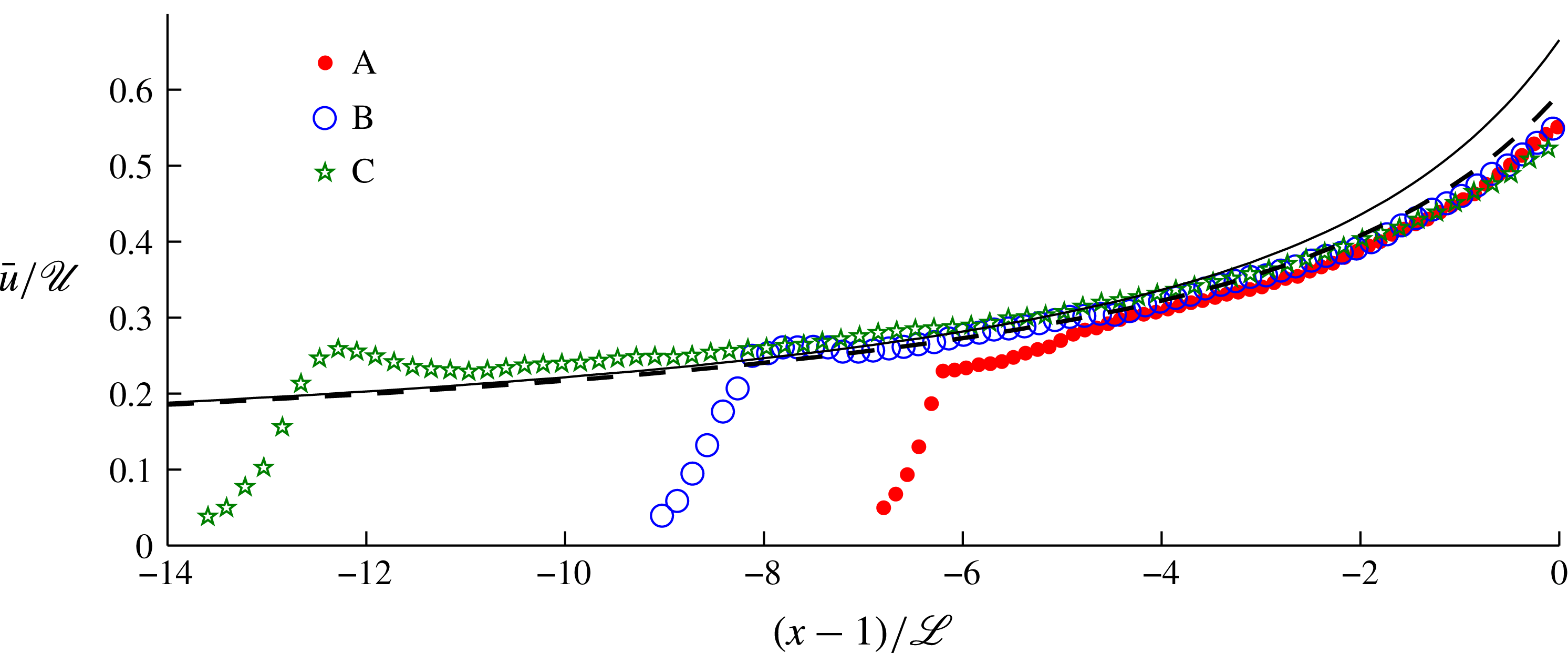
Experimental data for the profile of the width-averaged horizontal velocity
 $\bar{u}/\mathscr{U}$
plotted against the along-channel position relative to the channel exit
 $(x-l)/\mathscr{L}$
, each scaled by the relevant intrinsic scales of (3.2). The data were obtained using PIV for the three experiments listed in table 1. The prediction for the universal downstream profile
 $\hat{u} _{\ast }=1/{\hat{H}}_{\ast }$
with
 ${\hat{H}}_{\ast }$
given by (3.18) is shown as a solid curve. The alternative prediction of the revised theory of § 4.2 that includes the back-force from lateral extension at the channel exit is shown as a dashed curve. No fitting parameters have been used.

Parameter values used in the experiments arranged in order of ascending dimensionless channel length
 $L$
(a scaled horizontal aspect ratio).

The experiments were photographed at 2 s intervals from the top down using a digital SLR camera and terminated before the current made contact with the endwall of the tank. A photograph of a fully developed experiment is shown in figure 10. A sequence of side-view photographs showing the initial stages of an illustrative experiment designed to visualize the flow profile is shown in figure 11 and the supplementary movie, available at http://dx.doi.org/10.1017/jfm.2016.516. For this experiment, I implemented special visual considerations of dying the syrup using a red food colouring and omitting the upper layer of water. The sequence illustrates the development of an under-thick transition zone.
4.1 Experimental results
The experiments listed in table 1 spanned aspect ratios
 $l/w$
from 2 to 4, reduced gravities
 $g^{\prime }$
from 15.8 to
 $29.7~\text{cm}~\text{s}^{-2}$
and volumetric fluxes per unit width
 $Q$
from 0.037 to
 $0.052~\text{cm}^{2}~\text{s}^{-1}$
. The longitudinal and transverse components of the velocity field
 $(u,v)$
obtained using PIV of the images are shown in figure 12. The data indicate a qualitatively parabolic shear profile across the interior of the channel, with very slight transverse flow
 $v\approx 0$
. On reaching the mouth of the channel, the layer detaches from the sidewalls with a significant increase in lateral velocity
 $v$
reminiscent of a die swell from a tube (Tanner Reference Tanner2000). Downstream of the channel exit, the lateral velocity
 $v$
decays, the transverse profile becomes plug-like, and the flow continues to accelerate. Note that an apparent reduction in
 $u$
very close to the rim of the detached region is not physical and can be attributed to a failure of the PIV to resolve flow in a small region where the rim optically obscures the particles.
The final width-averaged longitudinal velocity along the channel
 $\bar{u}(x)$
is plotted as a function of the horizontal position with respect to the channel front,
 $x-l$
, for all three experiments in figure 13. The velocity and length are each scaled by the intrinsic scales
 $\mathscr{U}$
and
 $\mathscr{L}$
defined by (3.2). There is a good collapse of the data, indicating that the downstream flow is indeed universal up to scaling by the parameter groupings (3.2). The only significant differences between the sets of data occur near the backwall, where the flow is affected by the input. Overlaid on the data in figure 13 is the prediction of the universal profile
 $\hat{u} _{\ast }=1/{\hat{H}}_{\ast }$
(black solid curve), where
 ${\hat{H}}_{\ast }$
is the analytical solution (3.18). The prediction matches the data very well to within a scaled distance of two dimensionless units or about half a channel width (
 $2\mathscr{L}\approx 0.6w$
) upstream of the channel exit. A discrepancy with the data of approximately 20 % occurs at the channel exit itself.
4.2 Revised theory accommodating back-stress from the die swell
A striking feature of the experiment is the sharp increase in lateral velocity
 $v$
at the corners of the channel exit, which drives the die swell. This indicates a significant rate of transverse extension
 $\unicode[STIX]{x2202}v/\unicode[STIX]{x2202}y$
at the channel mouth. In the context of radially flowing extensional flows, the hoop stress due to lateral (azimuthal) extension of this kind was found to resist flow and generate back-stress (Pegler & Worster Reference Pegler and Worster2012). I anticipate that a similar back-stress arises here as a result of lateral extension at the channel exit and may explain the discrepancy between theory and experiment noted above.
To model this force, I retain the term involving transverse extension
 $\unicode[STIX]{x2202}v/\unicode[STIX]{x2202}y$
in the width integration of (2.13) to obtain the generalized frontal stress condition
 $$\begin{eqnarray}2\unicode[STIX]{x1D707}\left(2\frac{\unicode[STIX]{x2202}\bar{u}}{\unicode[STIX]{x2202}x}+\frac{1}{2s}[v]_{-s}^{s}\right)=\frac{\unicode[STIX]{x1D70C}g^{\prime }}{2}H\quad \text{at }x=l.\end{eqnarray}$$
With (4.2), the integration of the dimensional form of the steady-state equation (3.14) yields
 $$\begin{eqnarray}4H\frac{\text{d}\bar{u}}{\text{d}x}=\frac{\unicode[STIX]{x1D70C}g^{\prime }}{2\unicode[STIX]{x1D707}}H^{2}-\frac{C_{1}Q(l-x)}{s^{2}}-\frac{2v_{0}H(l)}{s},\end{eqnarray}$$
where
 $v_{0}\equiv v(l,s)$
. This is the same as the dimensional form of (3.15) but with the new, third term on the right-hand side representing the added resistive stress generated by lateral extension near the channel mouth. The lateral velocity
 $v_{0}$
is a new parameter, which I evaluate empirically as
 $v_{0}=\hat{v}_{0}\mathscr{U}$
with
 $\hat{v}_{0}\approx 0.22$
using the velocimetric data shown in figure 12(b). Using
 $u=Q/H$
to eliminate
 $u$
from (4.3) and then recasting it in terms of the dimensionless variables (3.3), I obtain the ordinary differential equation
 $$\begin{eqnarray}\frac{\text{d}{\hat{H}}}{\text{d}\hat{x}}=-\frac{1}{4}{\hat{H}}\left(\frac{1}{2}{\hat{H}}^{2}-(L-\hat{x})-\frac{2}{\sqrt{3}}\hat{v}_{0}{\hat{H}}(L)\right).\end{eqnarray}$$
I solved this equation subject to the matching condition (3.20a
) using a Runge–Kutta scheme in which
 ${\hat{H}}(L)$
is treated as a shooting parameter. The resulting velocity profile,
 $\hat{u} =1/{\hat{H}}$
, is plotted as a dashed curve in figure 13. The new prediction shows better agreement with the experimental data, indicating that the stresses due to lateral extension near the channel exit do indeed contribute to an appreciable reduction in the flow rate. According to the revised theory, the inclusion of the added resistive stress results in an 11 % reduction in the frontal flow rate from
 $\hat{u} (L)\approx 0.67$
given by (3.19b
), to
 $\hat{u} (L)\approx 0.60$
.
The surface profiles given by the solution to the steady-state system defined by (5.2) and (5.3) in the shear-thinning case corresponding to Glen’s law,
 $n=3$
, with channel length
 $L=5$
and a range of input thicknesses
 $D=0.2{-}\infty$
. Like the Newtonian case, the profiles adjust towards a universal profile (dashed blue curve) obtained by solving (5.2) numerically subject to (5.3b
) and the matching condition (5.5).

5 Generalization to power-law fluid
Motivated by the application to ice shelves, I generalize the steady-state results to allow for a power-law rheology. By considering scalings between all three force terms in (2.12) along with the scaling from the input-flux condition,
 $H\bar{u}\sim Q$
, I determine the general intrinsic scales of length, thickness and speed given by
 $$\begin{eqnarray}\mathscr{L}\equiv \left(\frac{s^{n+1}}{2^{n-1}(n+2)}\right)^{1/(n+1)}\!,\quad \mathscr{H}\equiv \left(\left[\frac{\unicode[STIX]{x1D707}_{0}}{\unicode[STIX]{x1D70C}g^{\prime }}\right]^{n}\frac{Q}{\mathscr{L}}\right)^{1/(n+1)}\!,\quad \mathscr{U}\equiv \left(\left[\frac{\unicode[STIX]{x1D70C}g^{\prime }Q}{\unicode[STIX]{x1D707}_{0}}\right]^{n}\mathscr{L}\right)^{1/(n+1)}\!,\end{eqnarray}$$
respectively. The scaling for the velocity (5.1c
) indicates that a larger power-law exponent
 $n$
(more shear thinning) increases the sensitivity of the flow to the parameter grouping
 $\unicode[STIX]{x1D70C}g^{\prime }Q/\unicode[STIX]{x1D707}_{0}$
but reduces sensitivity to the flow width
 $w$
contained in
 $\mathscr{L}$
. The raw scales in (5.1) are consistent with those obtained for
 $Q$
by Hindmarsh (Reference Hindmarsh2012).
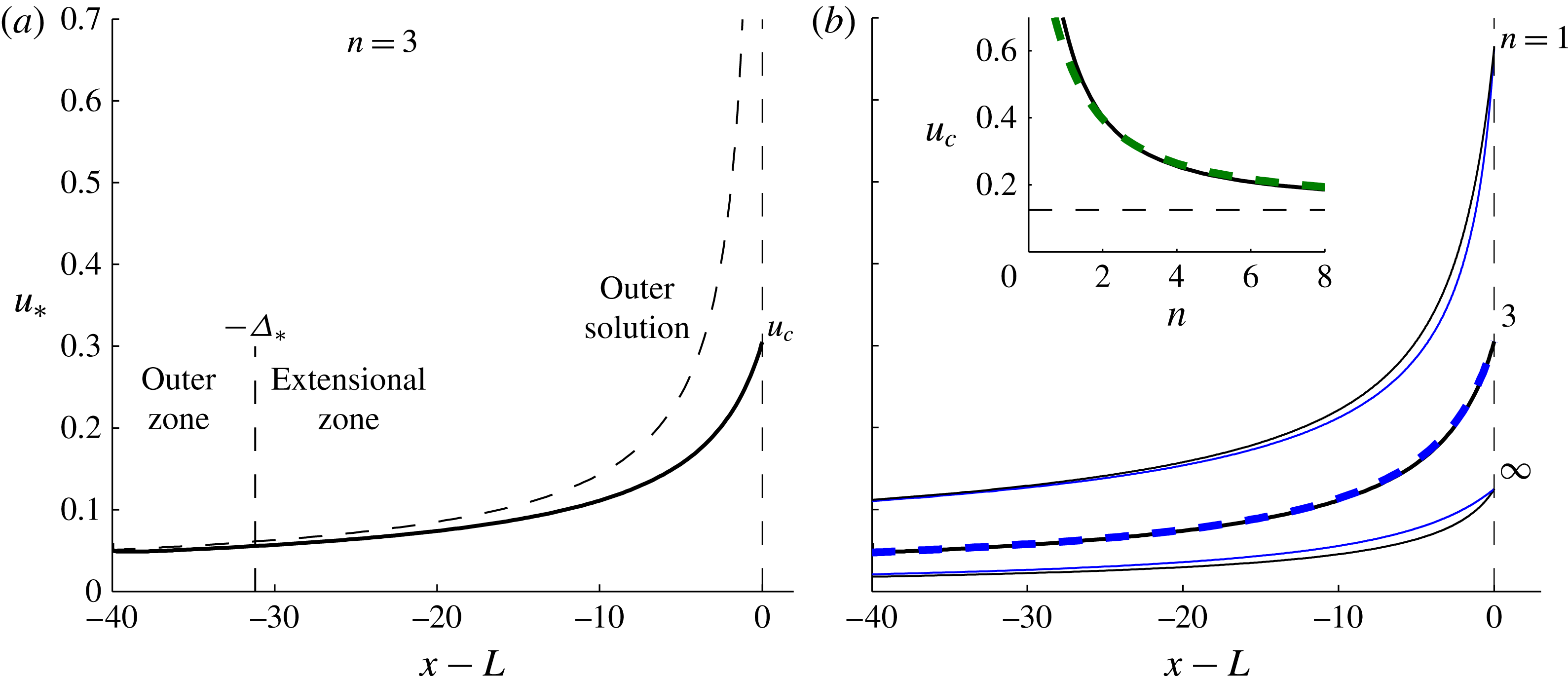
(a) The along-channel velocity of the universal profile
 $u_{\ast }(x)$
in the shear-thinning case
 $n=3$
, obtained from the numerical solution to (5.2) subject to (5.3b
) and (5.5). The outer solution based on neglecting extensional stresses (5.5) is shown by a dashed curve, and deviates significantly from the solution in a long boundary layer of extent
 $\unicode[STIX]{x1D6E5}_{\ast }\approx 31$
. (b) The universal profile
 $u_{\ast }(x)$
for a selection of power-law exponents
 $n=1,3$
and
 $\infty$
and their corresponding analytical approximations based on neglecting the divergence of extensional stresses (5.6a
) (blue). The inset of panel (b) shows the dimensionless frontal speed of the universal profile
 $u_{c}$
plotted against
 $n$
. Its analytical approximation (5.6b
) is shown as a dashed green curve. The asymptote
 $u_{c}\rightarrow 1/8$
as
 $n\rightarrow \infty$
is shown by a horizontal dashed line.

Using the steady form of the continuity equation
 $H\bar{u}=Q$
to eliminate
 $H$
in (2.12) and then recasting it in terms of dimensionless variables defined by (3.3) with (5.1), I obtain
 $$\begin{eqnarray}4\frac{\text{d}}{\text{d}x}\left(\frac{1}{u}\left|\frac{\text{d}u}{\text{d}x}\right|^{(1-n)/n}\frac{\text{d}u}{\text{d}x}\right)-u^{(1-n)/n}=\frac{1}{u}\frac{\text{d}}{\text{d}x}\left(\frac{1}{u}\right).\end{eqnarray}$$
The boundary conditions (3.1b ) and (2.17) become
 $$\begin{eqnarray}\displaystyle u(0)=D^{-1},\quad \frac{\text{d}u}{\text{d}x}(L)=\left(\frac{1}{8u(L)}\right)^{n}, & & \displaystyle\end{eqnarray}$$
where I have used
 $H=1/u$
to substitute for
 $H$
. The dimensionless input thickness and flow length are
 $$\begin{eqnarray}\displaystyle D\equiv \frac{d}{\mathscr{H}}\equiv \left(\left[\frac{\unicode[STIX]{x1D70C}g^{\prime }}{\unicode[STIX]{x1D707}_{0}}\right]^{n}\frac{\mathscr{L}}{Q_{0}}\right)^{1/(n+1)}\!\!d,\quad L\equiv \frac{l}{\mathscr{L}}\equiv k_{n}\frac{l}{w}, & & \displaystyle\end{eqnarray}$$
respectively, where
 $k_{n}\equiv [4^{n}(n+2)]^{1/(n+1)}$
.
The system defined by (5.2) and (5.3) was solved numerically using a Runge–Kutta scheme that marches forwards from the input condition (5.3a
) with the gradient
 $\text{d}u/\text{d}x$
at
 $x=0$
treated as a shooting parameter to meet condition (5.3b
). A selection of solutions with
 $n=3$
,
 $L=5$
and a large range of
 $D$
is shown in figure 14. The steady states adjust spatially towards a universal profile, analogously to the Newtonian case (cf. figure 5
b). The under-thick examples have much longer input transition zones than their Newtonian analogues, including pronounced regions of near-uniform thickness surrounding the turning points where
 $\text{d}H/\text{d}x=\text{d}u/\text{d}x=0$
. These arise because for
 $n>1$
the effective viscosity
 $|\text{d}u/\text{d}x|^{(1-n)/n}$
approaches infinity at the turning point, which is therefore surrounded by a plug-like region of high resistance and low deformation.
5.1 Solutions for the universal profile
In the Newtonian case
 $n=1$
, I determined the universal profile in § 3.3 using an asymptotic reduction of the analytical solution (3.16). With no exact solution of this kind generally available for
 $n\neq 1$
, I determine the universal profile in a different way by solving (5.2) numerically subject to (5.3b
) with the frontal value
 $u_{c}$
treated as a shooting parameter that is tuned to satisfy a condition of zero stress upstream,
 $\unicode[STIX]{x2202}u/\unicode[STIX]{x2202}x\rightarrow 0$
as
 $x\rightarrow -\infty$
. This zero-stress condition is equivalent to matching the flow to an outer region of drag-dominated flow, as was shown to be applicable to the Newtonian case in § 3.3.1. By neglecting the first term in (5.2), integrating it and then neglecting the constant of integration in the limit
 $L-x\gg 1$
, the outer solution is found to be
 $$\begin{eqnarray}u_{\ast }\sim [\unicode[STIX]{x1D6FC}(L-x)]^{-1/\unicode[STIX]{x1D6FC}}\quad \text{for }L-x\gg 1,\end{eqnarray}$$
where
 $\unicode[STIX]{x1D6FC}\equiv (n+1)/n$
, which generalizes (3.20b
) to non-Newtonian cases.
The numerically obtained universal velocity profile
 $u_{\ast }(x)$
for
 $n=3$
is shown as a solid curve in figure 15(a) and is compared alongside solutions for
 $n=1$
and
 $n=\infty$
(perfectly plastic) in figure 15(b). The profile is qualitatively similar to the Newtonian case shown earlier in figure 6, but the dimensionless speed at the channel exit
 $u_{c}\approx 0.305$
is just under half the value found for the Newtonian case, 0.666. The boundary of the extensional zone, defined as where
 $u_{\ast }$
deviates from the outer solution (5.5) by more than 10 %, is shown by a vertical dashed line in figure 15(a). It has the remarkably long extent
 $\unicode[STIX]{x1D6E5}_{\ast }\approx 31.2$
, corresponding to approximately 7 flow widths (
 $\unicode[STIX]{x1D6E5}_{\ast }\mathscr{L}\approx 7w$
). That is, the frontal discontinuity in depth-integrated pressure has a significant impact on flow 7 channel widths upstream of the front. This is much longer than the corresponding distance of just three-quarters of a channel width found for the Newtonian case (§ 3.3.1). One contributing factor to the significant difference is that
 $H_{\ast }(L)$
is more than twice as large with
 $n=3$
, indicating that shear thinning creates a larger frontal pressure discontinuity. The case
 $n=\infty$
is given by the exact solution
 $H=-4W_{-}(-2\text{e}^{x-2})$
, where
 $W_{-}$
is the lower branch of the Lambert
 $W$
function (the inverse of the function
 $f(z)=z\text{e}^{z}$
for
 $z\leqslant -1$
). The dimensionless frontal speed
 $u_{c}$
reduces with
 $n$
, as illustrated by the inset of figure 15(b). For
 $n=\infty$
, (5.3b
) implies that
 $u_{c}=1/8$
directly without any need to solve (5.2). In this case, the viscous stress at the channel front simply equals the yield stress specified by the constitutive law (2.4), and the frontal thickness
 $H_{\ast }(L)=8$
creates the discontinuity in depth-integrated frontal pressure needed to balance this uniform magnitude of stress.
While extensional stresses at the front of the channel have the potential to impact flow over a significant distance, its divergence in the governing equation, given by the first term on the left-hand side of (5.2), may be neglected to excellent approximation. This was demonstrated for a Newtonian fluid in § 3.3.1. To confirm it in non-Newtonian cases, I neglect the first term in (5.2) and integrate it to obtain
 $$\begin{eqnarray}\displaystyle u_{\ast }\approx [u_{c}^{-\unicode[STIX]{x1D6FC}}+\unicode[STIX]{x1D6FC}(L-x)]^{-1/\unicode[STIX]{x1D6FC}},\quad \text{where}~u_{c}\approx 8^{-\unicode[STIX]{x1D6FC}^{-2}} & & \displaystyle\end{eqnarray}$$
is an integration constant representing the speed at the flow front. I set the value of
 $u_{c}$
as the value obtained from my numerical solution. Alternatively, one could use the analytical approximation (5.6b
), which is obtained by substituting (5.6a
) into the frontal condition (5.3b
). The inset of figure 15(b) shows (5.6b
) as a dashed green curve, and agrees to good approximation with the numerically determined values of
 $u_{c}$
, as well as reproducing the convergence
 $u_{c}\rightarrow 1/8$
as
 $n\rightarrow \infty$
. The approximation (5.6a
) is shown as a blue curve alongside each of the three solutions in figure 15(b), showing good agreement in all cases. The approximation is especially accurate in the case of Glen’s law,
 $n=3$
, for which the maximum deviation from the exact solution is just 2 %, occurring at
 $x\approx L-5.1$
. In conclusion, while the balance of extensional stress at the flow front has a far-reaching effect on the upstream flow, the divergence of extensional stresses along the channel plays an insignificant role and the analytical approximations based on its neglect (5.6) are almost exact.
Speed map of the Amery Ice Shelf (data from Rignot et al. Reference Rignot, Mouginot and Scheuchl2011). The white arrows indicate the three primary glaciers feeding the ice shelf.

6 Application to ice shelves
The regime diagram of figure 8 partitions the space of dimensionless flow lengths
 $L$
(a scaled horizontal aspect ratio) and dimensionless input thicknesses
 $D$
into four regimes: those long enough for the asymptotic flow containing the universal profile to arise, those short enough for a purely extensional flow, and those containing an under-thick or over-thick input transition zone. This section considers the location of a few ice-shelf systems on the analogue of this diagram relevant to Glen’s law and thus assesses how widely the regime containing the universal profile arises in nature.
To illustrate a typical setting, a speed map of the Amery Ice Shelf is shown in figure 16 (data from Rignot et al. Reference Rignot, Mouginot and Scheuchl2011). The ice shelf is fed at the confluence of three glaciers indicated by white arrows and some smaller, tributary ice streams further downstream. Apart from the junctions with these ice streams, the flow along the edges of the channel is effectively stagnant. Approximately 500 km from the primary input, the ice shelf detaches from the confining edges of the channel. A further 50 km downstream lies its calving front. The features of no lateral slip and an approximately steady input and calving conditions are consistent with the modelling assumptions I have made.
Regime diagram showing the location of the ice shelves listed in table 2 in the space of dimensionless parameters
 $(D,L)$
. Bars indicate ranges arising from variation in the parameters along each ice shelf. Colour indicates the dimensionless frontal thickness
 ${\hat{H}}(L)$
predicted by the theory of § 5 for
 $n=3$
, and is the Glen’s law analogue of the colour plot of figure 8. The special value associated with the universal profile
 ${\hat{H}}_{\ast }(L)=3.28$
is shown white, under-thick cases red and over-thick cases blue. The thick curve separates over-thick and under-thick cases. The contours
 ${\hat{H}}(L)=(1\pm 0.1)3.28$
(thin, solid) represent the separation between short flows for which transition towards the universal profile does not complete (red and blue regions) and long flows for which it does (white regions). All the ice shelves lie in the long, over-thick region, for which the prevailing flow is predicted by the theory to be described by the universal profile calculated in § 5.1 and the frontal flow law (6.4) can be expected to apply.

Estimates of the thickness at the grounding line
 $d$
, cross-channel width
 $w$
, flow length
 $l$
and volumetric flux per unit width
 $Q$
for five ice-shelf regions. The given ranges encompass the variation in values for a given ice shelf. The implied dimensionless parameters (6.2) are given in the last two columns. The parenthetical values for
 $w$
correspond to the value at the calving front or point of lateral detachment. These were used to evaluate the theoretical prediction for the frontal flow rate (6.4), which is compared against geophysical data in figure 18.


6.1 Classification of ice-shelf regimes
In applying the theoretical results to ice shelves, I begin by estimating parameters. In accord with Glen’s law, the viscosity coefficient and power-law exponent are
 $$\begin{eqnarray}\displaystyle \unicode[STIX]{x1D707}_{0}={\textstyle \frac{1}{2}}A(T)^{-1/n}\quad \text{and}\quad n=3, & & \displaystyle\end{eqnarray}$$
respectively, where
 $A(T)$
is a temperature-dependent function (Cuffey & Paterson Reference Cuffey and Paterson2010). With the value
 $A\approx 3.8\times 10^{-25}~\text{Pa}^{-n}~\text{s}^{-1}$
suggested by Cuffey & Paterson (Reference Cuffey and Paterson2010),
 $\unicode[STIX]{x1D707}_{0}\approx 7\times 10^{7}~\text{Pa}~\text{s}^{1/n}$
. Given the density of glacial ice
 $\unicode[STIX]{x1D70C}\approx 917~\text{kg}~\text{m}^{-3}$
and ocean water
 $\unicode[STIX]{x1D70C}_{w}\approx 1027~\text{kg}~\text{m}^{-3}$
(Griggs & Bamber Reference Griggs and Bamber2011), the reduced gravity
 $g^{\prime }\equiv (\unicode[STIX]{x0394}\unicode[STIX]{x1D70C}/\unicode[STIX]{x1D70C}_{w})g\approx 1.05~\text{m}~\text{s}^{-2}$
.
The estimates of
 $\unicode[STIX]{x1D707}_{0}$
,
 $n$
,
 $\unicode[STIX]{x1D70C}$
and
 $g^{\prime }$
given above are characteristic of most ice shelves. Substituting these estimates into the dimensionless parameters (5.4a,b
), I obtain
 $$\begin{eqnarray}\displaystyle D=1.6\times 10^{-4}(w/Q)^{1/4}d\quad \text{and}\quad L=4.2(l/w), & & \displaystyle\end{eqnarray}$$
respectively. The grounding-line thickness
 $d$
, flow width
 $w$
, flow length
 $l$
and flux per unit width
 $Q$
can differ significantly between ice shelves. Using the velocimetric and topographic data from Griggs & Bamber (Reference Griggs and Bamber2011) and Rignot et al. (Reference Rignot, Mouginot and Scheuchl2011), I estimated the values of
 $d$
,
 $w$
,
 $l$
and
 $Q$
shown in table 2 for five ice-shelf configurations. Note that the Ross Ice Shelf is partitioned near its eastern edge by Roosevelt Island. To account for this, the ice shelf is considered in two components: its smaller eastern part, referred to as Ross (east); and its significantly larger western part, referred to as Ross (main). Since the flow width
 $w$
and grounding-line thickness
 $d$
are not all uniform for any given ice shelf, ranges for
 $w$
and
 $d$
are provided. The flux per unit width
 $Q$
was measured by evaluating the width average
 $Q=\int Hu\,\,\text{d}y/w$
over a series of nodes spanning each calving front.
Figure 17 shows the theoretically predicted dimensionless frontal thickness
 ${\hat{H}}(L)$
, obtained from my numerical solutions for
 $n=3$
in § 5, as a colour map over the parameter space
 $(L,D)$
, creating the Glen’s law analogue of figure 8. Again, white represents the special value associated with the universal profile, given by
 ${\hat{H}}_{c}\approx 3.28$
for
 $n=3$
, blue represents under-thick cases and red over-thick; the contour
 ${\hat{H}}(L)=(1\pm 0.1){\hat{H}}_{c}$
separates ‘long’ flows for which the transition to the universal profile completes and ‘short’ for which it does not. A long over-thick shelf generally occurs for
 $L>1$
which, in reference to (6.2b
), corresponds to lengths greater than one-third of a channel width,
 $l>w/3$
.
The parameter ranges estimated for each ice shelf are shown by the black lines in figure 17. All the ice shelves are found to lie firmly within the over-thick and long regions of the parameter space, for which they are predicted to contain prevailing regions of flow described by the universal profile. These results indicate that the universal profile is likely to arise widely in nature.
6.2 Comparison with the prediction for frontal flow rate
Based on the classification of the ice shelves in figure 17 as long, all can be expected to involve a complete adjustment to the universal profile. To test this, I compared the width-averaged frontal flow rates of the ice shelves listed in table 2 with the prediction associated with the universal profile, determined in § 5 as
 $$\begin{eqnarray}\displaystyle \bar{u}_{\ast }(l)=\hat{u} _{c}\mathscr{U} & = & \displaystyle 0.305\left(\left[\frac{\unicode[STIX]{x1D70C}g^{\prime }Q}{\unicode[STIX]{x1D707}_{0}}\right]^{n}\mathscr{L}\right)^{1/(n+1)}\end{eqnarray}$$
 $$\begin{eqnarray}\displaystyle & = & \displaystyle 4.8\times 10^{-5}(Q^{3}w)^{1/4},\end{eqnarray}$$
where the units are
 $\text{m}~\text{s}^{-1}$
and I have substituted the common values of
 $\unicode[STIX]{x1D70C}$
,
 $g^{\prime }$
and
 $\unicode[STIX]{x1D707}_{0}$
estimated in § 6.1 to yield the expression (6.4), which is dependent only on the frontal flow width
 $w$
and the input flux per unit width
 $Q$
. The prediction (6.4) is compared with observed values in the scatter plot of figure 18 for the five ice-shelf systems listed in table 2. In cases where the flow lies in lateral contact all the way up to the calving front, I used the transverse width at the calving front
 $w$
given by the parenthetical values in table 2. In the case of the Amery Ice Shelf, I instead used the value of
 $w$
measured at the point at which the ice shelf detaches from its sidewalls; the prediction is compared with the observed width-averaged flow rate at that location. There is generally good agreement, with excellent agreement in the cases of the Amery and Ronne Ice Shelves (a less than 4% discrepancy). A relatively larger overprediction of 19% occurs in the case of the Filchner Ice Shelf. The good agreement indicates that these ice shelves have all approached the universal profile obtained theoretically in § 5 and that (6.4) is describing their frontal flow rates correctly over a range of parameters.
6.3 Discussion regarding the input transition zone
The classification as over-thick is consistent with the morphology of most (if not all) ice shelves, which thin along their full length. Thickness data for the Ronne Ice Shelf shows that it thins from approximately 2000 m at the grounding line of a number of its feeding glaciers to 1000 m over a length scale of only a few tens of kilometres (see figure 3 of Griggs & Bamber Reference Griggs and Bamber2011). That is, the ice shelf halves in thickness within just 1 % of its total length. This provides some evidence for a localized region of significant spatial variation near the grounding line, which is consistent with an over-thick input transition zone.
Given the theoretical possibility of an under-thick regime, the fact that no ice shelves lie within that category is indicative of an underlying physical cause. I explain this observation on the basis that a grounding line is a dynamically free boundary that moves in response to thickening or thinning of the ice sheet. Its position is not prescribed at a fixed location as I have assumed in (3.1). An under-thick profile requires a relatively larger force to input (there is a larger back-stress exerted by the ice shelf in this case) and it is thus feasible that, were an under-thick flow to form, it would stimulate grounding-line migration to a new position in deeper water where an over-thick ice shelf forms more stably. That is, the grounding settles more stably at positions where the thickness of the ice sheet is closer to the separation between under-thick and over-thick situations (the thick curve in figure 17). Such a situation would be consistent with a mode of grounding-line migration controlled by the lateral drag exerted on the ice shelf (Pegler Reference Pegler2012; Pegler et al. Reference Pegler, Kowal, Hasenclever and Worster2013; Kowal, Pegler & Worster Reference Kowal, Pegler and Worster2016).
While migration of the grounding line may reduce the development of an input transition zone in a marine ice sheet, the imposition of a fixed source in other physical contexts may sustain a transition zone more readily. For example, the introduction of fluid over a steep weir, incline or backwall (as in my experiments) forces fluid to detach and float along a fixed position. This allows for an under-thick input if the thickness at which fluid is introduced is sufficiently small, as evidenced by my experiments (see figure 11). A mode of input of this kind corresponds more closely to that of molten glass during the float-glass process.
6.4 Model limitations
The dimensionless solutions I have obtained describe a broad range of aspect ratios and fluid-mechanical parameters. However, realistic ice shelves can involve more complicated sidewall structures than the rectangular geometry I have assumed. They can also be significantly affected by snowfall accumulation and basal melting, which alter the mass of the ice shelf along its length. These effects could be accommodated within the model of § 2 and would probably create a different profile from that determined in § 5. Variations in temperature and grain size also create inhomogeneities in the coefficient of viscosity (6.1a,b ). Another limitation is my assumption of a source that is evenly distributed across the width of the channel. Large ice shelves are typically fed by localized ice streams, which could result in more complex two-dimensional transitional flow in front of the grounding line. There is also the potential for error caused by the ad hoc nature of the parametrization of lateral stress (2.10). I have provided some validation of this parametrization for a Newtonian fluid by comparison with my experiments. Further validation could be obtained by comparison with the predictions of the full two-dimensional extensional flow equations (2.2)–(2.4) or data from a laboratory experiment involving shear-thinning fluid.
7 Conclusions
I have investigated, theoretically, experimentally and with geophysical comparisons, the dynamics of extensional viscous flows introduced into an open-ended channel. The central result is that sufficiently long flow lengths produce a prevailing steady-state flow that is of a universal dimensionless form with respect to the position at which confinement ends (the channel mouth or calving front of an ice shelf, for example). With power-law exponent
 $n$
, the width-averaged velocity profile associated with this universal flow is represented by the analytical approximation (5.6a,b
), which has the dimensional form
 $$\begin{eqnarray}\bar{u}(x)\approx \left(\frac{1}{k_{n}}\left[\frac{\unicode[STIX]{x1D70C}g^{\prime }Q}{\unicode[STIX]{x1D707}_{0}}\right]^{n}w\right)^{1/(n+1)}\left(\hat{u} _{c}+k_{n}\unicode[STIX]{x1D6FC}\frac{(l-x)}{w}\right)^{-n/(n+1)},\end{eqnarray}$$
where
 $k_{n}\equiv [4^{n}(n+2)]^{1/(n+1)}$
,
 $\unicode[STIX]{x1D6FC}\equiv (n+1)/n$
and
 $\hat{u} _{c}\approx 8^{-\unicode[STIX]{x1D6FC}^{2}}$
. The associated thickness profile is
 $H(x)=Q/\bar{u}(x)$
. The dependence of (7.1) on the position of the channel mouth or calving front
 $l$
contrasts significantly with the profile predicted by a purely extensional model applicable for short or unconfined ice shelves, which is completely independent of
 $l$
. This difference in dependence represents a fundamental switch in the dynamical balances and flow structures that apply between ice shelves of short and long flow lengths.
The universal profile represented by (7.1) contains a boundary-layer structure involving an outer region upstream in which the flow is dominated by transverse shear (given by neglecting
 $\hat{u} _{c}$
) connected to the flow front through a region in which extensional stresses have a leading-order role in controlling the flow (the extensional zone). The length of the extensional zone is approximately three-quarters of a flow width for Newtonian fluid but increases significantly to 7 flow widths in the shear-thinning case
 $n=3$
more relevant to glacial flow. For aspect ratios typical of ice shelves, the local pressure discontinuity along the calving front, represented by
 $\hat{u} _{c}$
in (7.1), thus has a significant long-range effect over the full flow length from calving front to grounding line. Despite this, the divergence of extensional stresses in the governing force balance is uniformly small along the full length of the universal profile. Neglect of this contribution yields accurate analytical approximations for the universal profile, which are represented by (7.1).
The possible steady-state flows were classified onto a regime diagram that partitions the space of dimensionless flow lengths (a scaled horizontal aspect ratio) and input thicknesses into ‘long’ flows for which the universal profile represented by (7.1) arises and ‘short’ flows for which the flow is instead characteristically similar to a purely extensional regime. A further partitioning was made between flows that adjust spatially towards the universal profile (7.1) by thinning (over-thick) and those that adjust by thickening (under-thick). The input transition zones through which these adjustments take place are relatively short and contain significant lengthways deformation and extensional stresses. Lateral stresses have a significant impact on flow even if the length is just a fraction of the width. In the case
 $n=3$
, for example, all over-thick inputs complete their transition to the universal profile if the length exceeds just one-third of a channel width.
Good agreement was found between the prediction of the universal profile (7.1) in the Newtonian case
 $n=1$
and data from a series of laboratory experiments in which the full two-dimensional flow field of a floating film of syrup was measured using PIV. The experimental flows showed significant lateral swelling beyond the channel exit. The resistive back-stress associated with this swelling contributes to a global reduction in flow rate along the length of the channel. The prediction of a revised theory that includes this contribution was found to be in better agreement with the data.
An analysis of the positions of a selection of ice shelves on the regime diagram applicable to Glen’s law with
 $n=3$
indicated that the ice shelves are all sufficiently long for the adjustment to the universal profile to complete. Validation of this hypothesis was provided by a good agreement between the frontal flow rate of these ice shelves and the prediction of the universal profile obtained by setting
 $x=l$
in (7.1). All the ice shelves lie in the over-thick region of the parameter space and a few lie close to the boundary between over-thick and under-thick cases. This is indicative of a mode of grounding-line control dominated by the drag exerted on the ice shelf in which the grounding line stabilizes at a position where the ice-shelf profile associated with the universal profile (7.1) intersects the underlying bedrock.
Acknowledgements
I am grateful to M. G. Worster for many helpful discussions on this work. I would also like to thank C. Schoof for helpful comments. I am also grateful to the technicians of the DAMTP laboratory for their contribution to preparing my experimental apparatus.
Supplementary movie
A supplementary movie is available at http://dx.doi.org/10.1017/jfm.2016.516.
Appendix A. Parametrization of the lateral shear stress
This appendix develops the parametrization of lateral stress (2.10) based on approximating the flow locally as a (shear-dominated) two-dimensional Poiseuille flow driven by an unknown pressure gradient
 $G(x)$
. In this regime, the
 $x$
component of the Stokes equation takes the form (Bird, Armstrong & Hassager Reference Bird, Armstrong and Hassager1987)
 $$\begin{eqnarray}\displaystyle \frac{\unicode[STIX]{x2202}\unicode[STIX]{x1D70E}_{xy}}{\unicode[STIX]{x2202}y}=G(x)\quad \text{or}\quad \unicode[STIX]{x1D70E}_{xy}=\unicode[STIX]{x1D707}\frac{\unicode[STIX]{x2202}u}{\unicode[STIX]{x2202}y}=G(x)y & & \displaystyle\end{eqnarray}$$
on integration subject to a condition of symmetry along
 $y=0$
. Substituting the effective viscosity (2.4) into (A 1b
) under an assumption of shear-dominated flow, I obtain
 $$\begin{eqnarray}\tilde{\unicode[STIX]{x1D707}}_{0}\left|\frac{\unicode[STIX]{x2202}u}{\unicode[STIX]{x2202}y}\right|^{(1-n)/n}\frac{\unicode[STIX]{x2202}u}{\unicode[STIX]{x2202}y}=G(x)y,\end{eqnarray}$$
where
 $\tilde{\unicode[STIX]{x1D707}}_{0}\equiv 2^{1-(1/n)}\unicode[STIX]{x1D707}_{0}$
. Integration of (A 2) subject to the no-slip condition (2.5a
) yields
 $$\begin{eqnarray}\displaystyle u=\left[\frac{-G(x)}{2\tilde{\unicode[STIX]{x1D707}}_{0}}\right]^{n}\frac{(s^{n+1}-|y|^{n+1})}{(n+1)}\quad \text{and}\quad \bar{u}=\left[\frac{-G(x)}{2\tilde{\unicode[STIX]{x1D707}}_{0}}\right]^{n}\frac{s^{n+1}}{(n+2)}. & & \displaystyle\end{eqnarray}$$
Using (A 3b
) to evaluate
 $G(x)$
in (A 1b
) and setting
 $y=s$
, I obtain (2.10).