2.1. Linear stability and quasilinear impurity transport analysis

How the impurity transport is affected by the driven gyrokinetic electrostatic instabilities of a set of specific LHD impurity hole discharges can be found in Mikkelsen et al. (Reference Mikkelsen, Tanaka, Nunami, Watanabe, Sugama, Yoshinuma, Ida, Suzuki, Goto and Morita2014). However, a similar analysis is not reported, to our knowledge, for W7-X geometry, which motivates us to perform a quasilinear characterization of the turbulent impurity transport in this device prior to turning to the fully nonlinear treatment in § 2.2. In addition, recent work by Helander & Zocco (Reference Helander and Zocco2018) has analytically deduced some qualitative features of the quasilinear transport coefficient of impurities, which can be contrasted with the presented quasilinear numerical estimations.

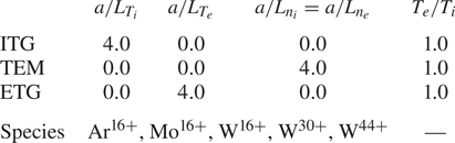
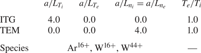
The selected parameters and impurity species for the quasilinear study are summarized in table 1. The gradients of the bulk species have been set such that hybrid instabilities were discarded. That is, $\{a/L_{T_i}, a/L_{T_e}, a/L_{n_e}\}=\{4, 0, 0\}$ has been set for the ITG driven instability, $\{a/L_{T_i}, a/L_{T_e}, a/L_{n_e}\}=\{0, 0, 4\}$ for density gradient driven TEMs, and $\{a/L_{T_i}, a/L_{T_e}, a/L_{n_e}\}=\{0, 4, 0\}$ for ETG modes.Footnote ³ This election is based on the typical gradient scales measured at the edge of W7-X plasmas, see e.g. Geiger et al. (Reference Geiger, Wegner, Beidler, Burhenn, Buttenschön, Dux, Langenberg, Pablant, Pütterich and Turkin2019). In particular, normalized temperature gradients larger than $4.0$ are commonly observed in enhanced performance scenarios induced by auxiliary pellet fuelling (Baldzuhn et al. Reference Baldzuhn, Damm, Beidler, McCarthy, Panadero, Biedermann, Bozhenkov, Brunner, Fuchert and Kazakov2019; Bozhenkov et al. Reference Bozhenkov, Kazakov, Ford, Beurskens, Alcusón, Alonso, Baldzuhn, Brandt, Brunner and Damm2020). Although a density gradient of approximately $4.0$ may be more characteristic of the far edge than of the simulated radial position, $r/a=0.7$, setting it equal to the temperature gradients follows from the intention of comparing the contribution with the radial impurity transport produced by the different instabilities at equal size of their driving gradient. For all cases the flux tube has been extended three turns poloidally, the wavenumber along the radial direction has been set to $k_x=0$, and the wavenumber along the binormal direction, $k_y$, has been scanned. All simulations have been performed with kinetic main ions, electrons and a single impurity species at a trace concentration. The set of selected impurities have included $\textrm {Ar}^{16+}$, $\textrm {Mo}^{16+}$, $\textrm {W}^{16+}$, $\textrm {W}^{30+}$ and $\textrm {W}^{44+}$.

Table 1.

Normalized gradients, electron to ion temperature ratio and selected impurities considered for the quasilinear transport study.

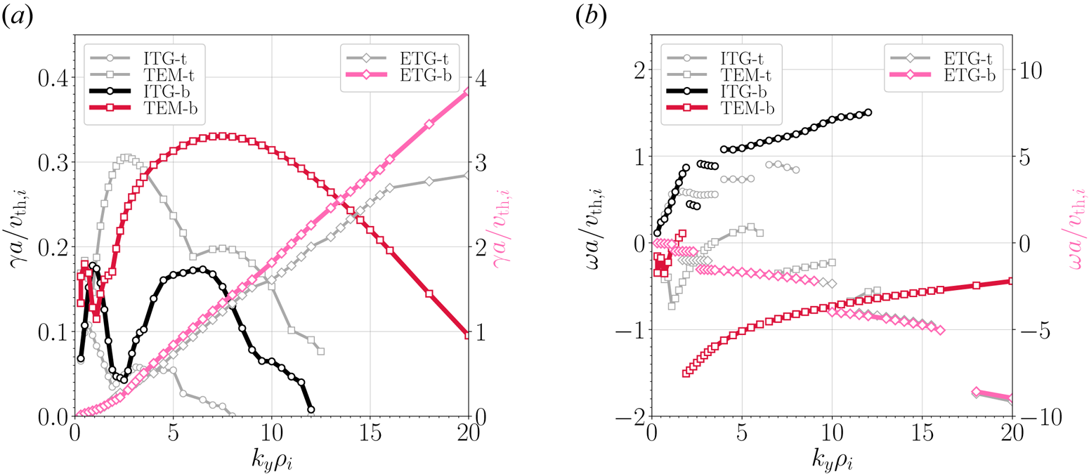
For the bean and triangle flux tubes, the spectra of the growth rate, $\gamma$, and frequency, $\omega$, for the three different linear instabilities simulated are represented in figure 1(a) and figure 1(b), respectively. For the three instabilities, figure 1(a) shows that the bean flux tube develops more unstable modes along the whole $k_y$ range than the triangle flux tube. Focusing then on the bean flux tube, it is observed that the ITG-driven instability features a double peak structure and extends over a considerably broad $k_y$ range up to $k_{y}\rho _i\approx 12$. However, the fastest growing mode is located at $k_{y}\rho _i\approx 1$. Changes in the dominant eigenmode can be inferred from the discontinuous spectrum of the frequency. The sign of the frequency indicates that the modes rotate in the ion diamagnetic direction for all $k_y$. On the other hand, the density gradient driven TEM is found to be more unstable than the ITG, with the fastest growing mode of the former featuring a growth rate a factor of two larger than that of the latter. The fastest growing mode is located at $k_y\rho _i\approx 7.5$, although the instability extends beyond $k_y\rho _i=20$. The sign of the frequency indicates that the mode can rotate both in the ion diamagnetic direction for the low $k_y$ part of the spectrum, and in electron diamagnetic direction at moderate and high $k_y$. Finally, the ETG-driven instability shows a monotonic increase of the growth rate towards electron Larmor scales, not covered on the simulated range of $k_y$, where the most unstable $k_y$ is expected to be located. 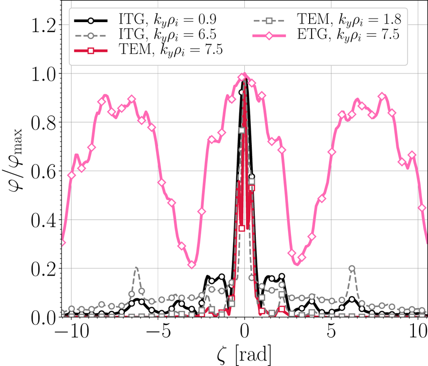Note, though, the large value of the growth rate (referred to the right-hand $y$-axis) that the ETG-driven instability develops at scales of a few ion Larmor radii. The frequency, in this case, shows that the mode rotates in the electron diamagnetic direction and that different branches, presumably dominated by a different eigenmode, are encountered, as the discontinuous frequency pattern points out. Finally, figure 2 represents for the bean flux tube the parallel structure of the most unstable ITG and TEM modes, with $k_y\rho _i=0.9$ and $k_y\rho _i=7.5$, respectively, as well as that of the ETG mode with $k_y\rho _i=7.5$. For comparison, the eigenfunctions of the ITG and TEM mode corresponding to the second local maximum of the growth rate, located in figure 1(a) at $k_y\rho _i=6.5$ and $k_y\rho _i=1.8$, respectively, are also represented. The figure reveals the strong localization of the TEM and the ITG instabilities around the centre of the bean flux tube, although the latter presents a comparatively greater spread-parallel structure than the former. On the other hand, the ETG exhibits by far the most extended structure, without any predominant localization at a specific region along the parallel coordinate.

Figure 1.

For the bean (thick coloured lines) and the triangle (thin grey lines) flux tubes, normalized growth rate (a) and frequency (b) as a function of the normalized binormal wavenumber $k_y$ for the three sets of background unstable conditions considered for the quasilinear impurity transport study, namely, ITG driven by $a/L_{T_{i}}=4.0$ (circles), TEM driven by $a/L_{n_{e}}=a/L_{n_{i}}=4.0$ (squares) and ETG driven $a/L_{T_{e}}=4.0$ (diamonds). Here, the normalization uses the ion Larmor radius, $\rho _i$, the ion thermal speed, $v_{\text {th},i}$ and the effective minor radius, $a$.

Figure 2.

For the bean flux tube: eigenfunctions of the ITG modes (circles) corresponding to the two local maxima of the ITG growth rate spectrum represented in figure 1; eigenfunctions of the TEMs (squares) corresponding to the two local maxima of the TEM growth rate spectrum represented in figure 1; eigenfunction of the ETG mode with $k_y\rho _i=7.5$ (diamonds). For the ITG and TEM cases, the coloured solid lines correspond to the most unstable mode and the grey dashed lines correspond to the second local maximum of their growth rate spectra.

Returning to the question about the impurity transport driven by the above-mentioned instabilities, we have followed the same approach as in Mikkelsen et al. (Reference Mikkelsen, Tanaka, Nunami, Watanabe, Sugama, Yoshinuma, Ida, Suzuki, Goto and Morita2014). Given a mode with wavenumbers $k_x$ and $k_y$, the linear Vlasov–Poisson gyrokinetic system of equations is solved for each simulated time step, and the gyroaveraged impurity distribution $g_Z(k_x, k_y,z,v_{\|}, \mu , t)$ and electrostatic potential $\varphi (k_x, k_y,z, t)$ are obtained. From these two quantities, the flux surface averaged impurity flux, $\varGamma _Z(k_x,k_y, t)$, is computed. Note that, once the instability has been triggered the electrostatic potential $\varphi$ and, consequently, $\varGamma _Z$ grows exponentially. However, a quasilinear mixing-length estimate of the flux,

(2.2)\begin{equation} \varGamma^{ql}_{Z}(k_x, k_y, t)=\frac{\varGamma_{Z}(k_x, k_y, t)\gamma(k_x, k_y, t)} {n_Z\left\langle\varphi^2(k_x, k_y,z, t)\right\rangle k_\bot^2(k_x,k_y)}, \end{equation}

can be defined, so that a well-converged quantity is obtained once the growth rate is stabilized. In this expression $\left \langle \cdots \right \rangle$ denotes the flux surface average operator and $k_\bot =k_x\boldsymbol {\nabla } x+k_y\boldsymbol {\nabla } y$. Considering $k_x=0$ for all simulations, for each impurity species in the presence of a background instability, the $k_y$-spectrum of the quasilinear flux has been extracted at the last simulated time step. This process has been repeated with three different pairs of impurity density and temperature gradients, in order to obtain from each impurity species embedded in a different type of instabilities the spectra of the three transport coefficients.

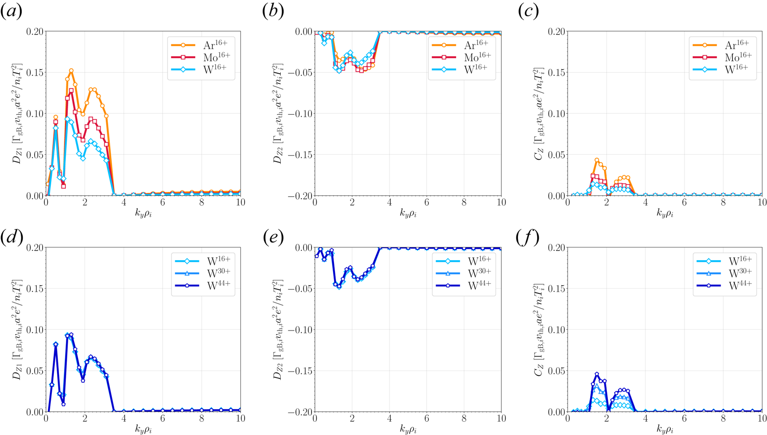
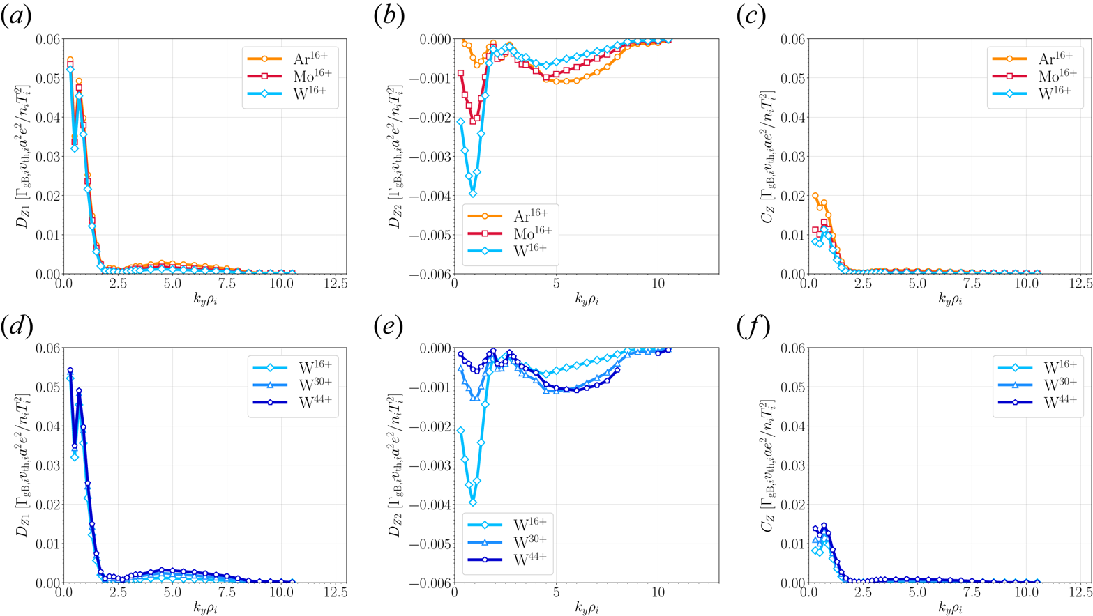
For the ITG instability, the spectra of the diffusion coefficient, $D_{Z1}$, thermodiffusion coefficient, $D_{Z2}$ and the impurity flux in the absence of impurity density and temperature gradients, $C_Z$, are displayed on the left-hand, centre and right-hand columns of figure 3, respectively. While the panels (a–c) show the results for the selected impurities with different mass, panels (d–f) do the same for the impurities with different charges. In first place, $D_{Z1}$ turns out to be roughly one order of magnitude larger than $D_{Z2}$, each having a different sign. That is, while diffusion drives impurities downhill the density profile, thermodiffusion would add an inward convection contribution, assuming a peaked impurity temperature profile. In any case, this contribution seems very weak. Another inward contribution to the flux arises at vanishing impurity density and temperature gradients, which, however, also seems comparatively small compared with the size of $D_{Z1}$. The spectra of the three transport coefficients show that most contributions to the total flux come from the lowest part of the spectrum, from $k_y\rho _i\lesssim 1.5$. Finally, no significant dependence on the impurity charge or mass is observed for $D_{Z1}$ and $C_Z$. On the other hand, the size of the weak $D_{Z2}$ is larger with increasing mass and decreasing charge.

Figure 3.

For the ITG case (see table 1), $k_y$-spectra of the diffusion coefficient $D_{Z1}$ (a,d), thermodiffusion coefficient $D_{Z2}$ (b,e) and pinch in the absence of gradients $C_{Z}$ (c, f) for the different impurities, for a mass (a–c) and charge (d–f) scan. The values are given in normalized units, with $\varGamma _{\text {gB},i}$ the gyro-Bohm ion particle flux, $v_{\text {th},i}$ the ion thermal speed, $e$ the unit charge, $a$ is the effective minor radius and $n_i$ and $T_i$ the main ion density and temperature, respectively.

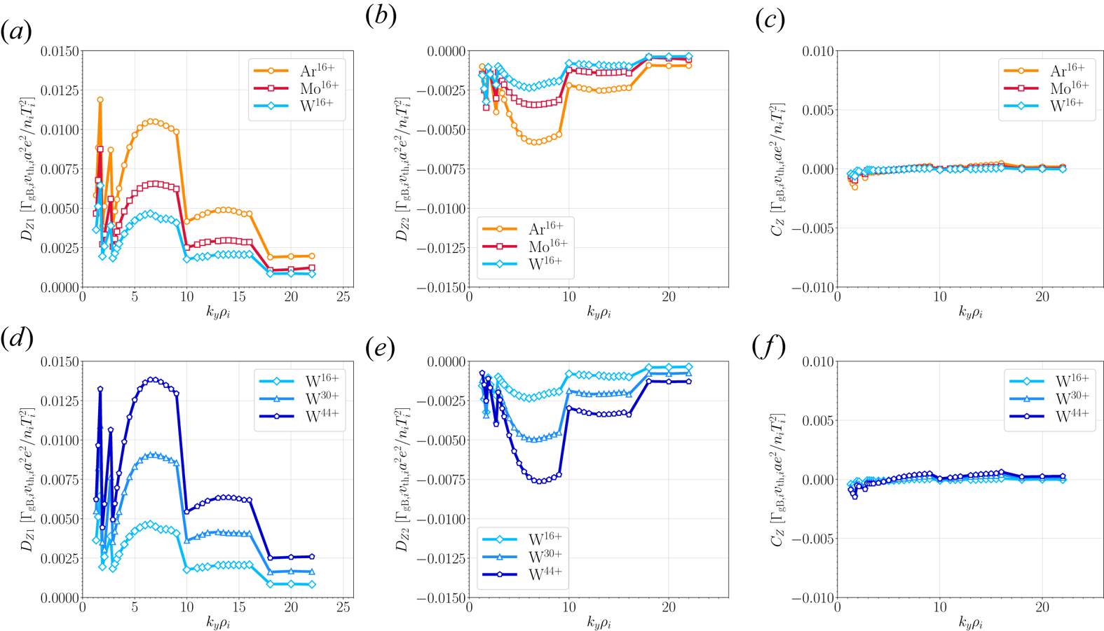
For the impurity transport coefficient driven by TEM instability, the corresponding results are shown in figure 4. In general, the transport coefficients follow the same trends as those observed in the ITG case. The diffusion coefficient is, in absolute value, larger than the thermodiffusion, and the sign of each of them is the same as for the ITG instability. However, the difference between $D_{Z1}$ and $D_{Z2}$ is a factor of three, while in the ITG case they differed by roughly one order of magnitude. Furthermore, the strength of $D_{Z1}$ in this case is enhanced with respect to the ITG mode, possibly due to the more unstable character of this TEM, see figure 1. Furthermore, the three coefficients exhibit broader $k_y$-spectra than in the ITG case. Regarding the dependence of the coefficients on the mass or the charge, it is observed that $D_{Z1}$ somewhat depends on the charge and that $C_Z$ also depends on the charge and the mass.

Figure 4.

For the TEM case, see table 1, $k_y$-spectra of the diffusion coefficient $D_{Z1}$ (a,d), thermodiffusion coefficient $D_{Z2}$ (b,e) and pinch in the absence of gradients $C_{Z}$ (c, f) for the different impurities, for a mass (a–c) and charge (d–f) scan.

Finally, the results concerning the ETG instability are represented in figure 5. In contrast to the ITG and TEM cases, $D_{Z1}$ is not particularly larger than $D_{Z2}$ in absolute value, and both are, in any case, considerably smaller than in the previous two cases. In addition, $C_Z$ is practically zero, which indicates that ETG driven impurity transport should be substantially smaller compared with that driven by the ITG mode or the TEM.

Figure 5.

For the ETG case, see table 1, $k_y$-spectra of the diffusion coefficient $D_{Z1}$ (a,d), thermodiffusion coefficient $D_{Z2}$ (b,e) and pinch in the absence of gradients $C_{Z}$ (c, f) for the different impurities, for a mass (a–c) and charge (d–f) scan.

In summary, the quasilinear approach to the problem has delivered the following conclusions. Both ITG and TEM should drive most of the impurity transport by ordinary diffusion. The ITG mode seems to be prone to developing slightly peaked impurity density profiles, as $C_Z$ and $D_{Z2}$ are considerably smaller than the dominant $D_{Z1}$ and both add inward convective contributions to the total flux. The TEM case follows roughly the same characteristics, although $C_Z$ and $D_{Z2}$ are not as small compared with the diffusion coefficient $D_{Z1}$, which points out the tendency to develop peaked impurity density profiles with larger gradients than in the ITG case. In general, the sign and size of the transport coefficient are in reasonably good agreement with the analytical predictions (Helander & Zocco Reference Helander and Zocco2018). For instance, comparing the absolute value of $D_{Z1}$ for the three instability types, represented on the left-hand column of figures 3, 4 and 5, with the size of $D_{Z2}$, shown on the central column of those figures, it is found that $|D_{Z2}|$ is considerably smaller than $|D_{Z1}|$. The sign of $D_{Z2}$ also matches the quasilinear analytical prediction. The main differences between our results and those analytically derived reside on the mass or charge dependence of our results, which arises from the fact that all terms, including the parallel streaming neglected on the analytical treatment of Helander & Zocco (Reference Helander and Zocco2018), are retained in our simulations. For that reason too, the pinch in the absence of gradients in the present work, $C_Z$, is not strictly comparable to the so-called curvature pinch of the cited quasilinear analytical treatment.

2.2. Nonlinear turbulent transport of trace impurities

Quasilinear analyses allow us to extract qualitative information about the more or less prominent role of an instability in the turbulent impurity flux, the relative size of the different diffusive and convective terms, the direction, inward or outward, of the flux driven through each transport coefficient, and its wavenumber spectra. However, quasilinear calculations cannot provide a quantitative estimation of the flux, as nonlinear simulations do, since no saturated state is reached. While nonlinear multispecies gyrokinetic simulations have been employed with remarkable success for tokamaks – see for instance Barnes, Parra & Dorland (Reference Barnes, Parra and Dorland2012) for a comprehensive study of the scaling of the impurity transport of particles, momentum and energy – in stellarators they are anecdotal. In the present section, the question about the size of the turbulent impurity transport driven by ITG- and TEM-driven microturbulence and the respective transport coefficients is addressed by means of nonlinear simulations. Three of the impurities considered in the previous section, $\textrm {Ar}^{16+}$, $\textrm {W}^{16+}$ and $\textrm {W}^{44+}$, have been selected. Each simulation includes hydrogen nuclei, electrons and one single impurity species, all three kinetically treated. For the ITG case the resolution has been set to $N_z\times N_x\times N_y\times N_{v_{\|}}\times N_{\mu }=96\times 76\times 151\times 24\times 12$, while for the TEM turbulence $N_z\times N_x\times N_y\times N_{v_{\|}}\times N_{\mu }=96\times 76\times 256\times 48\times 12$ has been taken. The width of the box along the binormal and radial directions has been set to $L_y=125\rho _i$ and $L_x=180\rho _i$, respectively, and the flux tube has been extended one turn poloidally. Standard twist-and-shift boundary conditions (Beer, Cowley & Hammett Reference Beer, Cowley and Hammett1995) have been considered. In table 2 the parameters considered for the background turbulence of interest in each case is indicated, together with the selected impurities.

Table 2.

Normalized gradients, electron to ion temperature ratio, and selected impurities considered for the nonlinear transport analysis.

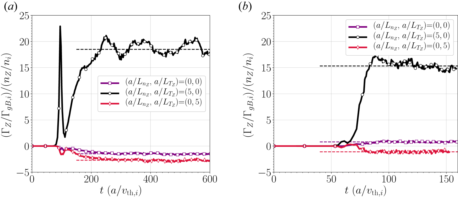
In order to obtain the transport coefficients, $D_{Z1}$, $D_{Z2}$ and $C_Z$, for each impurity and type of background turbulence, three simulations have been performed with different values of impurity normalized density and temperature gradients, $a/L_{n_Z}$ and $a/L_{T_Z}$, respectively. As an example, the three time traces of the turbulent flux of $\textrm {Ar}^{16+}$ are illustrated for the ITG case in figure 6(a) and for TEM turbulence in figure 6(b). For each of them, the mean value of the flux during the saturated phase is represented by a dashed line. Looking at the flux evolution when the impurity density and temperature gradients are zero (open squares linked by the purple solid line), it is immediately observed that each type of turbulence drives, in the absence of impurity density and temperature gradients, flux contributions with opposite sign. While ITG drives an inward (pinch) contribution, TEM turbulence drives outward transport (anti-pinch). Note that this first observation contradicts the quasilinear results, where in both cases $C_Z$ was positive, thus it drove negative flux for all $k_y$. However, that contribution is weak, and comparable to that arising when the temperature gradient is non-zero (open diamonds connected by the red solid line). On the other hand, the flux driven when only the density gradient is applied (open circles connected by the black solid line) is by far the largest, no matter if the background turbulence is ITG- or TEM-driven, which anticipates that ordinary diffusion will be the dominant contribution to the turbulent particle flux of impurities, as it will be quantitatively confirmed below for the other two impurity species considered.

Figure 6.

Normalized $\textrm {Ar}^{16+}$ particle flux as function of time in the presence of ITG-driven (a) and TEM-driven (b) background turbulence. The result is represented for three different pairs of Ar$^{16+}$ density and temperature gradients: $(a/L_{n_Z}, a/L_{T_Z})=(0,0)$ (squares); $(a/L_{n_Z}, a/L_{T_Z})=(5,0)$ (circles); $(a/L_{n_Z}, a/L_{T_Z})=(0,5)$ (diamonds).

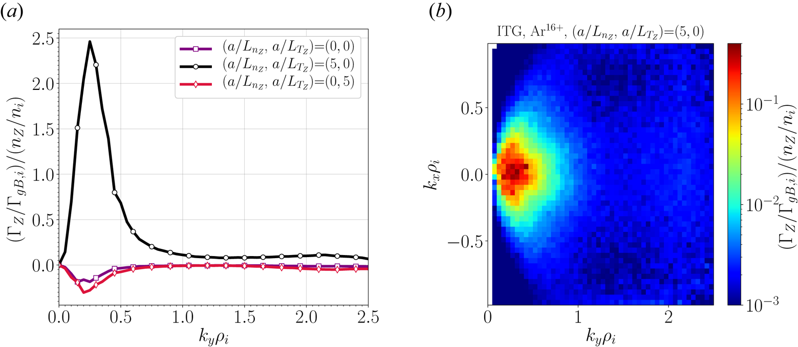
Given the width of the linear growth rate spectra of the simulated ITG and TEM modes, see figure 1, one might wonder if the turbulent flux spectra are that broad or if the chosen resolution does not leave important flux contributions out of the selected range of wavenumbers. For the case of $\textrm {Ar}^{16+}$ embedded in ITG microturbulence, the binormal wavenumber spectrum is represented for the three simulated pairs of impurity density and temperature gradients in figure 7(a). It can be seen that most of the flux contribution arises from large scales with $k_{y}\lesssim 1$, although finite contributions can also be observed for the remaining part of the spectrum. This is particularly visible when the impurity density gradient is the only gradient applied (open circles connected by the black solid line). Regarding the radial wavenumber spectrum, figure 7(b) shows the spectrum $k_x$ and $k_y$ of the $\textrm {Ar}^{16+}$ converged flux. As for the ITG-driven turbulence, the largest contributions to the flux arise from a narrow region of large radial scales, with maximum contribution along $k_x=0$. Although not shown here, these features are found with little variation for the rest of estimated fluxes under ITG conditions, independently of the impurity species.

Figure 7.

For ITG microturbulence: (a) $k_y$-spectrum of the normalized turbulent flux of $\textrm {Ar}^{16+}$ considering $(a/L_{n_Z}, a/L_{T_Z})=(0,0)$ (squares), $(a/L_{n_Z}, a/L_{T_Z})=(5,0)$ (circles), $(a/L_{n_Z}, a/L_{T_Z})=(0,5)$ (diamonds); (b) $(k_x,k_y)$-spectrum of the normalized turbulent flux of Ar$^{16+}$ when $(a/L_{n_Z}, a/L_{T_Z})=(5,0)$.

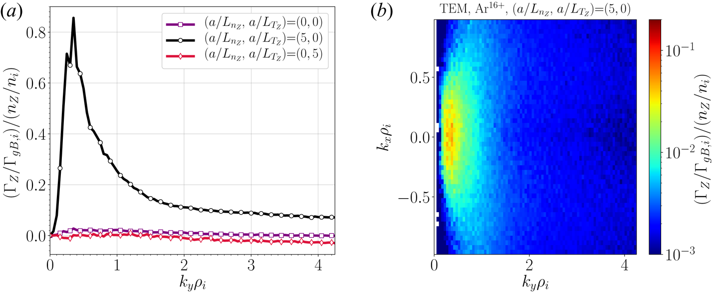
The equivalent two plots for the three simulations performed for Ar$^{16+}$ in the presence of TEM microturbulence are shown in figure 8. Panel (a), representing the binormal flux spectrum, reveals qualitative differences compared with the corresponding figure of the ITG case discussed in the previous paragraph, figure 7(a). Looking at the $k_y$-spectrum of the flux when $a/L_{n_Z}=5$, it is obvious that TEM turbulence leads to a noticeably broader flux spectrum. Although the flux of $\textrm {Ar}^{16+}$ finds its largest contribution at scales with $k_y\rho _i\approx 1$, the spectrum decays for increasing wavenumber less abruptly than in the ITG example. This yields appreciable flux contributions even at the largest $k_y$ represented. Concerning the radial direction, figure 8(b) depicts, for the case $a/L_{n_Z}=5$, the flux spectrum in $k_x$ and $k_y$, that exhibits a wider $k_x$ range with noticeable flux contributions than in the ITG case as well. Finally, regarding the much weaker flux driven in the absence of impurity density and temperature gradients, although difficult to appreciate due to the much smaller amplitude, no significant contributions to the flux are present for $k_y\gtrsim 2$. In contrast, when the impurity temperature gradient is set to a finite value, the flux spectrum slightly diverges as $k_y$ increases. It is worth noting that in that case two small contributions, connected to the thermodiffusion driven pinch and the anti-pinch in absence of gradients, are opposing to each other (see discussion about figure 6b), which may require a finer resolution than the one considered.

Figure 8.

For TEM microturbulence: (a) $k_y$-spectrum of the turbulent particle flux of $\textrm {Ar}^{16+}$ considering $(a/L_{n_Z}, a/L_{T_Z})=(0,0)$ (squares), $(a/L_{n_Z}, a/L_{T_Z})=(5,0)$ (circles), $(a/L_{n_Z}, a/L_{T_Z})=(0,5)$ (diamonds); (b) $(k_x,k_y)$-spectrum of the turbulent particle flux of Ar$^{16+}$ when $(a/L_{n_Z}, a/L_{T_Z})=(5,0)$.

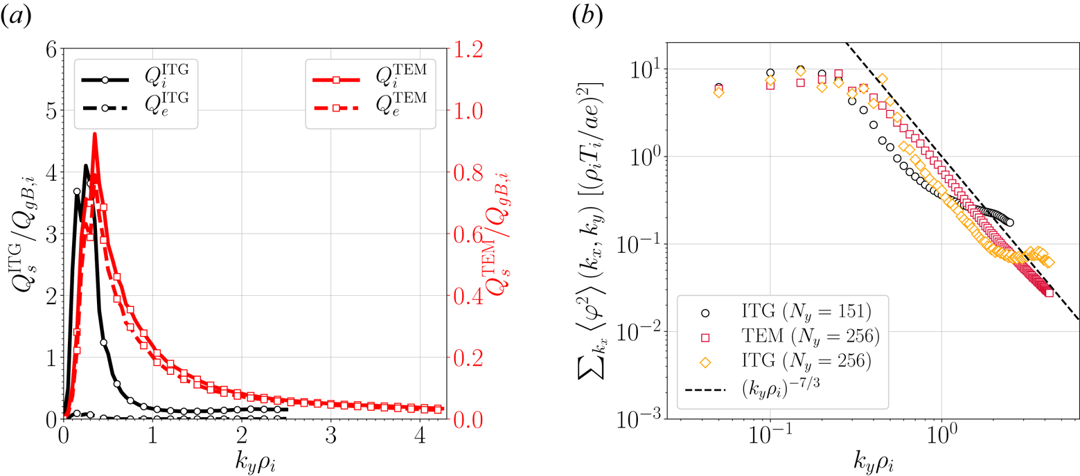
Despite the better delimitation of the ITG-driven impurity flux spectra within the considered wavenumber window in comparison with the TEM case, it is important to emphasize that other properties of interest of the background turbulence are equally well captured by both ITG and TEM simulations. Such is the case of the bulk ion and electron heat fluxes, whose spectra are represented in figure 9(a). Similarly to the impurity particle flux, the heat flux spectra are broader for the TEM case than for the ITG case. However, figure 9(a) demonstrates that, for the estimation of the heat fluxes, regardless of the type of turbulence and the species under consideration, there is margin to consider a narrower $k_y$ range. With regard to the features that figure 9(a) illustrates, it is worth noting the comparable bulk ion and electron heat fluxes driven by the TEM turbulence and the practically negligible electron heat flux compared with the ion heat flux driven by the ITG turbulence. Another quantity of interest for the background turbulence is the electrostatic fluctuation spectrum, which is represented, for the two types of turbulence considered throughout this section, in figure 9(b). It can be immediately appreciated how TEM turbulent electrostatic fluctuations (open red squares) tightly follow a power law with exponent -7/3. For the ITG turbulence, the same power law is followed up to $k_y\rho _i\approx 1$, and deviates for larger values of $k_y\rho _i$. Note that this deviation is just a matter of resolution, as it shows up at lower $k_y$ values for the choice $N_y=151$ (open black circles) than for the finer resolution of $N_y=256$ (open orange diamonds). A specific investigation about why the ITG-driven particle flux spectra seem to be better bound by our mode window than for the TEM case, while the energy cascade is better converged for the TEM than for the ITG case, is beyond the scope of the present paper. But, in any case, this parenthetical remark leaves us the important conclusion that both ITG and TEM microturbulence in W7-X are intrinsically three-dimensional, as demonstrated in Barnes, Parra & Schekochihin (Reference Barnes, Parra and Schekochihin2011).

Figure 9.

(a) Normalized bulk ion and electron heat flux spectra driven by the ITG turbulence (referred to the left-hand $y$-axis) and the TEM turbulence (referred to the right-hand $y$-axis). (b) Electrostatic fluctuation spectrum for the ITG and TEM turbulence considered for the nonlinear impurity transport calculations. Note the selected resolution choices for the transport simulations considered $N_y=151$ and $N_y=256$ for the ITG (open black circles) and TEM (open red square), respectively. A third case is considered here, an ITG run with $N_y=256$ (open orange diamonds) for comparison. The dashed line indicated the power law $(k_y\rho _i)^{-7/3}$.

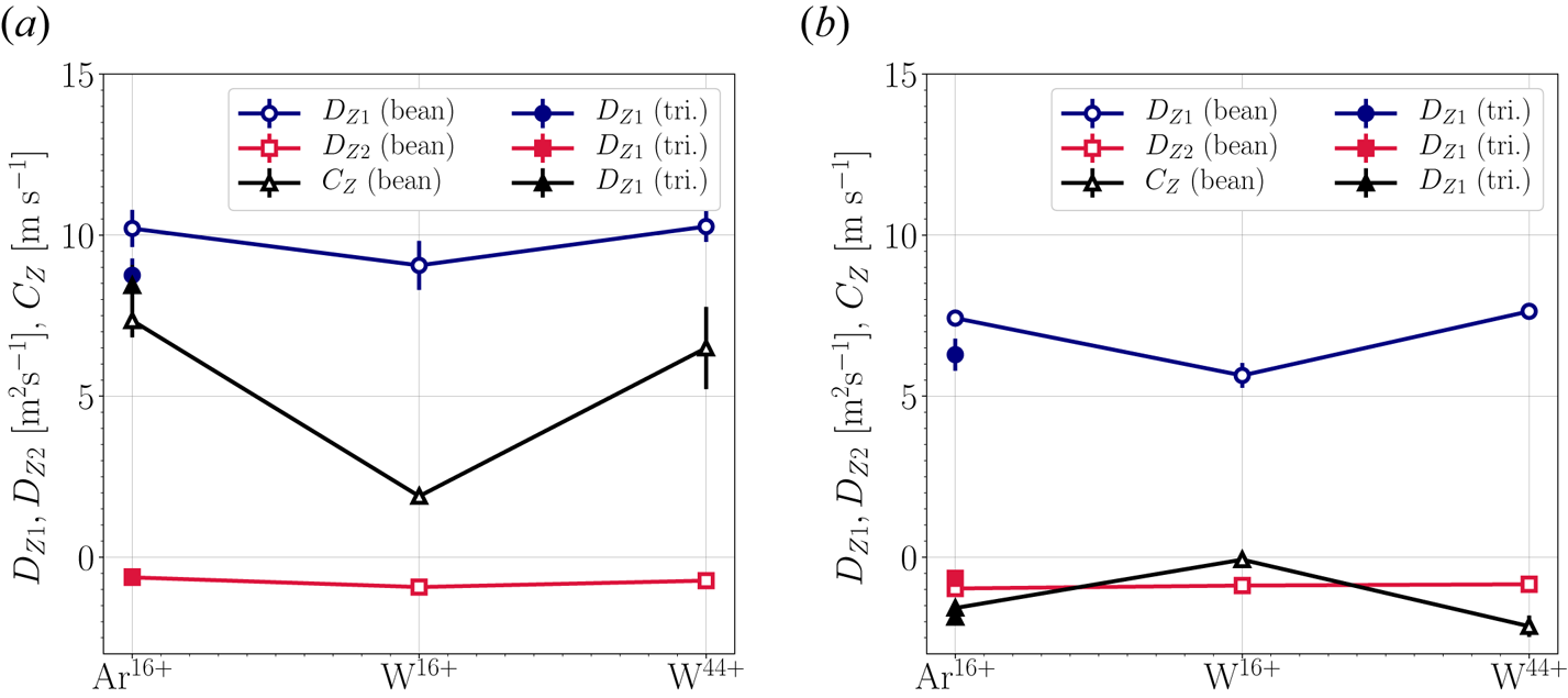
Returning to the question about the size of the transport coefficients of different impurities under the influence of different type of turbulence, figure 10 represents the ordinary diffusion coefficient, the thermodiffusion coefficient and the flux in the absence of impurity and density gradient of $\textrm {Ar}^{16+}$, $\textrm {W}^{16+}$ and $\textrm {W}^{44+}$ embedded in ITG microturbulence, figure 10(a), and in TEM microturbulence, figure 10(b). Note that all calculations have been performed considering the bean flux tube and, for Ar$^{16+}$, the triangle flux tube as well. The reference electron density and ion temperature values considered are $n_e=10^{19}\ \textrm {m}^{-3}$ and $T_i=T_Z=1$ keV, respectively. Some features common to both cases are: (i) the dominance of the diffusion coefficient, $D_{Z1}$, above the other two coefficients, reaching values of around $10\ \textrm {m}^2\ \textrm {s}^{-1}$ and $6\text {--}7 \ \textrm {m}^2\ \textrm {s}^{-1}$ for ITG and TEM turbulence, respectively; (ii) $D_{Z2}$ is substantially smaller than $D_{Z1}$ and adds a pinch contribution (assuming peaked $T_Z$ profiles) to the radial transport of the three species under investigation; (iii) ordinary diffusion and thermodiffusion are practically independent on the mass and the charge state, however, the absolute value of $C_Z$ is reduced appreciably for $\textrm {W}^{16+}$, possibly related to its smaller charge to mass ratio compared with that for the other two impurities; (iv) in both cases, moving to the triangle flux tube yields, for $\textrm {Ar}^{16+}$, a reduction of $D_{Z1}$, although not particularly strong, a negligible modification of $D_{Z2}$ and a slight increase of the absolute value of $C_{Z}$. The only features that are clearly different for the ITG and the TEM cases are related to $C_Z$: (i) the positive sign of $C_Z$ adds a pinch contribution in the ITG case, while the negative sign of $C_Z$ for the TEM case contributes to expulse impurities (see expression (2.1)); (ii) the absolute value of $C_Z$ is noticeably larger for ITG than for TEM. Of all these features, it is worth mentioning that the large relative size of $D_{Z1}$ or the low size and sign of $D_{Z2}$ are qualitative characteristics advanced by the quasilinear analysis. On the other hand, the relative strength between the ITG- and TEM-driven $D_{Z1}$ as well as the sign and size of $C_Z$ for the TEM turbulence are not captured by the quasilinear simulations.

Figure 10.

For the bean flux tube (open dots), diffusion coefficient, $D_{Z1}$, thermodiffusion coefficient, $D_{Z2}$ and flux at vanishing $T'_Z$ and $n'_Z$, $C_Z$, for $\textrm {Ar}^{16+}$, $\textrm {W}^{16+}$ and $\textrm {W}^{44+}$ in the presence of ITG (a) and TEM (b) microturbulence. For comparison, the values of the transport coefficients of $\textrm {Ar}^{16+}$ obtained for the triangle flux tube are represented with filled dots. Reference density and temperature values of $n_e=10^{19}\ \textrm {m}^{-3}$ and $T_i=T_Z=1$ keV have been considered.

Finally, it is important to recall that the equilibrium impurity density gradient is determined by the value of the peaking factor, which is expressed as the ratio of the total convection velocity, $V$, and the diffusion coefficient $D$. In terms of the three coefficients under discussion, the peaking factor reads as

(2.3)\begin{equation} \frac{V}{D}=-\frac{D_{Z2} \,\text{d}\ln T_Z/\text{d} r +C_Z}{D_{Z1}}. \end{equation}

In practical terms, the numerical demonstration of the large diffusion coefficient just shown yields the conclusion that microturbulence, of the ITG and TEM kind, should tend to form impurity density profiles close to flatness.Footnote ⁴ For instance, for the values shown in figure 10(a) the resulting peaking factor in equilibrium, although negative for ITG background conditions, would reach large absolute values only if the impurity temperature gradient were unrealistically strong. The peaking factor would be even weaker in the presence of TEM turbulence, since it exhibits a rather weak anti-pinch at vanishing $T'_Z$ and $n'_Z$ together with a pinch contribution of comparable size driven by thermodiffusive processes, which would in the end lead to a peaking factor fairly close to zero. On the other hand, the fact that $C_Z$ results in an outward contribution to the flux opens the possibility that TEM drives hollow impurity density profiles, and motivates a deeper investigation of the properties of this pinch on the magnetic configuration space of W7-X.

2.3. Nonlinear turbulent transport of non-trace impurities

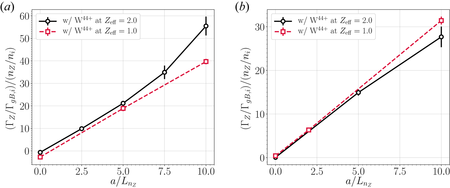
All the calculations up to this section have considered impurities at trace concentration, so that they responded to the background turbulence driven by the bulk species gradients without affecting that turbulence. In that situation, the flux of the impurities scales linearly with their density and temperature gradients, the impurity transport coefficients are constant as long as the background turbulence is not altered, and they can be obtained by employing expression (2.1). Nonetheless, in laboratory plasmas impurities are frequently present at non-trace concentration levels, and the assumption of impurity turbulent fluxes scaling proportionally to the impurity density and temperature gradients does not necessarily hold. For this reason, the present subsection touches on the question of how much the tendency of the impurity flux deviates from linear when the impurity concentration is no longer negligible. It is not the intention of the present section to provide a detailed study including several species and different background turbulence, as done in § 2.2 for the nonlinear analysis for trace impurities. The purpose is rather to shed some light that indicates to what degree the conclusions drawn in § 2.2 can be extrapolated for realistic impurity content. We have performed a series of simulations considering $\textrm {W}^{44+}$ at a concentration such that the effective charge is $Z_{\text {eff}}=2$. Only the impurity density gradient has been scanned, keeping $a/L_{T_{Z}}=0$, as we have seen that density gradient drives the dominant contribution to the turbulent flux of impurities. The resulting normalized turbulent fluxes of W$^{44+}$ are represented in figure 11(a) for the ITG-driven background turbulence and in figure 11(b) for the TEM case. For the curves representing the flux of $\textrm {W}^{44+}$ at $Z_{\text {eff}}=2$, it can be observed that the deviation from the linear trend is only noticeable at rather large normalized density gradient values, larger than $a/L_{n_Z}\approx 5$. This deviation is more obvious for the ITG case than for the TEM, and each of them points to opposite effects: while the TEM-driven turbulent transport of tungsten tends to be weakened with respect to the linear behaviour, the ITG-driven flux is enhanced. Apart from that, the presence of non-trace tungsten introduces an offset with respect to the linear trend in the ITG case, that is not found for the TEM. In other words, the presence of tungsten at non-trace concentration is altering the value of the ITG-driven pinch in the absence of tungsten density and temperature gradients towards making it nearly zero, as can be noted looking at the two points represented for $a/L_{n_Z}=0$. In any case, a closing remark from these simulations is that, unless $Z_{\text {eff}}$ is much larger than $2$, the dependence of the impurity fluxes on the impurity density gradient seems close enough to linear so that the conclusions drawn in § 2.2 can be extrapolated to moderately realistic values of $Z_{\text {eff}}$.

Figure 11.

Normalized radial particle flux of $\textrm {W}^{44+}$ as a function of its normalized density gradient at trace concentration (open squares) and at a concentration that makes $Z_{\mathrm {eff}}=2.0$ (open circles), for ITG (a) and TEM (b) microturbulence.