I. INTRODUCTION
In the past few years, increased efforts have been made in the development of microwave sensors for the characterization of biological tissues and liquids. Compared to conventional methods, e.g. X-rays, the main advantage of microwaves is the non-ionizing nature of the interaction with biological cells. Also, in contrast to low-frequency sensor systems, e.g. as used for impedance spectroscopy, the electromagnetic waves can penetrate the cells and thus give information on the properties of the cytoplasm and, in turn, the “inner” state [Reference Schwan1].
In order to perform measurements at cell scale both broadband and narrowband sensors using evanescent fields have been tested. The former include transmission line [Reference Booth, Orloff, Mateu, Janezic, Rinehart and Beall2] and capacitive [Reference Chen, Dubuc, Poupot, Fournie and Grenier3] sensors. In the latter case, resonators of various shapes are used [Reference Ferrier, Romanuik, Thomson, Bridges and Freeman4, Reference Chretiennot, Dubuc and Grenier5]. Another resonant technique uses substrate-integrated near-field sensors [Reference Ambrozkiewicz and Jacob6], which are the basis for this work.
Microwave near-field sensors have been proposed for different applications. The details can be found in several reviews [Reference Anlage, Talanov and Schwartz7, Reference Rosner and van der Weide8]. Most of the sensor systems include complex structures, fine sensing tips, and involved positioning procedures [Reference Tselev, Anlage, Christen, Moreland, Talanov and Schwartz9].
Another approach for near-field measurements, in particular for those on biological cells, is to integrate the sensing tip with a microfluidic channel leading the cell past the sensor for scanning. However, single cells are quite small (diameter of ~15 µm); therefore, microsystem technology is required for manufacturing of useful sensor designs. Nonetheless, proof-of-principle investigations can be performed at a larger scale.
This is also the scope of the present contribution. A planar sensor is described with a very simple structure, which can be translated to microsystem manufacturing. The sensor structure is described in Section II and radiation effects are discussed in Section III. An approach for the quantitative evaluation of measurement data is proposed and evaluated in Section IV.
II. SENSING DEVICE
A) Circular half-mode resonators
Substrate-integrated waveguides are used for different passive components such as filters [Reference Hong and Gong10, Reference Huang and Chen11], couplers [Reference Zhai12], slot antennas [Reference Sanz Izquierdo, Young, Grigoropoulos, Batchelor and Langley13], and near-field sensors [Reference Haase and Jacob14]. Using multiple dielectric layers and a multilayer process, various structures can be realized. Common to all substrate-integrated components is the replacement of vertical metal walls with via fences. These can be designed in such a way that radiation to the sides is negligibly small [Reference Grigoropoulos, Sanz-Izquierdo and Young15, Reference Uchimura, Takenoshita and Fujii16].
The sensors proposed here are based on a folded circular half-mode resonator. The principle of the latter was first introduced in [Reference Haase and Jacob17]. The half-mode waveguides are used for a coupler design in [Reference Zhai12]. The steps needed to develop a half-mode resonator are described in Fig. 1. The fundamental mode of a cylindrical cavity can be folded along a symmetry plane of the magnetic field (cross-section) without a strong influence on the resonant frequency and the quality factor (Q-factor). The folding step leads to a field distribution as sketched in Fig. 1(b). As the symmetry plane corresponds to an open circuit, the upper layer of the resonator can be removed, leading to an equivalent half-mode resonator [Reference Haase and Jacob17].
Folding steps of a circular waveguide cavity with sketched field distributions. (a) Circular cavity, horizontal and vertical cross section (b) Folded cavity, and (c) Folded half-cavity.

In previous publications, different substrate-integrated near-field sensors of the closed type, i.e. with both top and bottom half have been analyzed, based on folded rectangular [Reference Ambrozkiewicz and Jacob6], square [Reference Haase and Jacob14, Reference Haase and Jacob18], and circular resonators [Reference Haase and Jacob19], respectively. The advantage of the half-mode sensors is their simple structure and thus the low manufacturing cost.
Instead of the half-circle obtained by folding a circular cavity also sectors, e.g., a quarter, an eighth, or a sixteenth circle can be considered because of the field symmetry. It was shown in [Reference Haase and Jacob19] that this detunes the resonance and lowers the Q-factor. This is due to the transition from the cavity mode to a quarter-wave transmission line resonance. The sensitivity of the multiple-folded sensors was shown to increase with each folding step. The best compromise between high sensitivity and an acceptable Q-factor are the quarter and the eighth circle sensors, respectively.
B) Circular half-mode near-field sensor
Based on the results in [Reference Haase and Jacob17] and [Reference Haase and Jacob19], two different sensors are analyzed in the following sections. To realize a sensor based on the half-mode resonator, a sensing tip is attached at the corner on the top layer, which corresponds to the center of the original circular resonator. The electric field, which is maximum there, extends to the tip and a strongly localized evanescent field is generated.
The resonator is connected via two inductive coupling loops. In order to evaluate the resonance from a transmission measurement, the coupling is chosen to be weak (maximum transmission below −20 dB). The sensors are shown in Fig. 2. They are referred to as Sensor 1 and Sensor 2 in the following, in accordance with the figure. The main difference is the angle of the resonator φ res which is 90° for Sensor 1 (quarter circle) and 45° for Sensor 2 (eighth circle). The radius r res is adjusted to tune the sensors to the same resonant frequency. It is 11.0 mm for Sensor 1 and 10.4 mm for Sensor 2. The remaining parameters indicated in Fig. 2 are identical for both sensors and are: g = 0.8 mm, l tip = 2.3 mm, w tip = 0.2 mm, s tip = 0.1 mm, and l front = 0.33 mm in the tip region and w line = 0.7 mm, s line = 0.15 mm, and w loop = 0.1 mm at the feed line. The vias have a radius r via = 0.25 mm and a spacing d vias ≈ 0.9 mm around the resonators and up to 1.6 mm for the port vias. The thickness of the substrate is h sub = 0.8 mm.
Quarter- and eighth-circle half-mode sensors.
Owing to the open folding gaps, the coupling loops, and the sensing tip, there is some radiation. Its dependence on the sensor geometry and sample properties is analyzed in more detail in Section III.
C) Operating principle
The sensor functions as follows: a sample is placed in a given volume on top of the sensing tip. In the case of a liquid sample this can be defined by a reservoir or a channel. The sample, being placed in the vicinity of the maximum electric field, detunes the resonator, i.e., its resonant frequency f r and Q-factor. In the case of high loss materials such as water, the effect of the sample on the resonance may be quite involved. For some sensors [Reference Chretiennot, Dubuc and Grenier5], it is possible to describe the resonant frequency as a linear function of the relative permittivity ε r, while the inverse of the Q-factor is proportional to the loss tangent tanδ of the sample. For the sensors proposed here, this is not possible due to the strong interaction with the sample as was found in a full-wave simulation. Therefore, both resonant frequency and quality factor depend on both material parameters, i.e. permittivity and loss tangent.
The advantage of the strong interaction is of course high sensitivity with respect to the sample properties.
As a matter of illustration, some resonance curves from a systematic parameter sweep are shown in Fig. 3. For the simulation the full-wave solver Ansys HFSS [20] is used. A realistic model of the sample and its reservoir is employed. Details are given in Section II-D.
Simulated sensor response to changes in permittivity or loss tangent of the sample. (a) Sensor 1, constant permittivity ε r = 64 (b) Sensor 1, constant loss tangent tanδ = 0.2 (c) Sensor 2, constant permittivity ε r = 64, and (d) Sensor 2, constant loss tangent tanδ = 0.2.
The cross-dependencies mentioned above are more pronounced for Sensor 2. This makes qualitative statements on the sample properties difficult, because the changes of one of the sample properties can mask the effect of the other one.
However, using a suitable calibration, quantitative results can be obtained for a complex sample permittivity despite the cross-dependencies. One method is described in Section IV.
D) Liquid sample reservoir
The sensors are manufactured on a Rogers RO4003C substrate using a standard chemical etching process. The cylindrical reservoir for the liquid samples is milled into a block of acrylic glass. It is glued to the substrate with a conventional all-purpose glue in such a way that the sensing tip protrudes into the bottom of the reservoir by l p. A sketch of the geometry in the vicinity of the sensing tip is shown in Fig. 4. The values of the indicated parameters are listed in Table 1, they are the same for both sensors. In the simulation, the following values are assumed for the permittivity of the materials. The substrate Rogers RO4003C has ε r,s = 3.55 and tanδ s = 0.0027, the acrylic glass ε r,a = 3.4 and tanδ a = 0.001, and the glue ε r,g = 3.5 and tanδ g = 0.04.
(A) Top and (B) side view of a cylindrical acrylic glass reservoir on a sensing tip. Geometrical data are given in Table 1.
Geometrical data of liquid reservoir and tip–sample overlap (mm).

III. RADIATION
Owing to the open structure there will be some radiation. It can be quantified by means of a Q-factor analysis. The overall Q-factor is defined as [Reference Balanis21]
 $$Q = \displaystyle{{\omega _r W} \over {P_L }}\comma$$
where ω r = 2πf r is the angular resonant frequency of the resonator, W is the total stored energy, and P L is the dissipated power. The dissipation is caused by three mechanisms, i.e., dielectric and conduction loss P dc, radiation P rad, and coupling loss P ex. Therefore, three quality factors can be defined as
 $$\displaystyle{1 \over {Q_1 }} = \displaystyle{{P_{dc} + P_{rad} + P_{ex} } \over {\omega _r W}} = \displaystyle{1 \over {Q_{dc} }} + \displaystyle{1 \over {Q_{rad} }} + \displaystyle{1 \over {Q_{ex} }}.$$
In the case of weak coupling, the loaded and the external Q-factors Q 1 and Q ex, can be determined from the transmission coefficient, using a 3 dB bandwidth and the magnitude of maximum transmission [Reference Kajfez, Chebolu, Abdul-Gaffoor and Kishk22]. In the case of a non-radiating structure, Q dc can be evaluated. However, if the structure radiates, another step must be taken: as proposed in [Reference Mongia, Ittipiboon and Cuhaci23], a metal box can be used to shield the structure. In that case, no energy can be radiated, Q rad is infinitely large and thus Q dc can be measured. It can be assumed that the effect of the shield on Q dc is small, since the fields are weak outside the resonator. After removing the shield Q rad can be evaluated from the loaded Q of the open structure.
The power radiated in relation to the power dissipated in the structure is
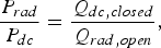 $$\displaystyle{{P_{rad} } \over {P_{dc} }} = \displaystyle{{Q_{dc\comma closed} } \over {Q_{rad\comma open} }}\comma$$
which can be used as a figure of merit for the sensors.
The radiation of Sensors 1 and 2 is determined in simulation and measurement using air and water samples. This illustrates the difference in radiation between the two sensor geometries and also between the different samples.
The simulated boundaries representing the front and the top side of the housing, shown in Fig. 5, are chosen as either radiating or perfectly electrically conducting for the open and shielded case, respectively. The permittivity of the water sample is described by a Debye model [Reference Stogryn24] to take the dispersion into account. The sample shape is chosen according to the measurement setup, where the sample is fixed on the sensing tip in the cylindrical reservoir described in Section II-D. The measurement setup is described in detail in Section V. The manufactured sensor in the housing and the shielding cover are shown in Fig. 5(a). The cover can be attached to the housing so as to avoid air gaps. Figure 5(b) shows a close-up view of the sample reservoir.
Photographs of Sensor 1. Geometry parameters are given in Table 1. (a) Sensor in housing and cover, (b) sample container.
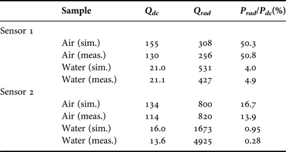
The calculated quality factors of the measured and the simulated structures are presented in Table 2. The most remarkable observation is the decreased radiation for water samples in comparison to air samples. In the case of Sensor 1, the measured (simulated) radiation is reduced from 50.8% (50.3) to 4.9% (4.0). For Sensor 2, this effect is similar. The radiation is lowered from 13.9% (16.7) to less than 1%. The decrease of radiation can be explained by the absorption of the water sample, which is placed at the location of maximum electric field. At 5 GHz the permittivity of water has a loss tangent of about 0.25 [Reference Kaatze25].
Quality factors for air and water samples, simulated and measured data.
Considering the discrepancies between measurement and simulation, two main reasons can be singled out. The surface roughness of the copper layers and the finite conductivity of the shielding cover (aluminum) can only be approximated in the simulation. The surface roughness of the copper on the substrate material is included in the simulation according to the data given by Rogers Corp. [26] by means of an effective conductivity. The finite conductivity of the aluminum cover reduces the Q-factor of the closed sensor. However, according to the simulation, the fields at the cover are low compared to those in the resonating structure. Thus, the effect on the Q-factor should also be low.
In addition, the Q-factor depends critically on the exact shape of the sensor, especially at the sensing tip. The shape and position of the sample can only be approximated, though. Nonetheless, the comparison between measurement and simulation generally shows a reasonable agreement concerning radiation. The most prominent outlier in Table 2 is the measured Q rad of Sensor 2 with water as a sample. The measured Q-factors are nearly equal with and without shielding which leads to a high value of Q rad.
In conclusion, the analysis shows that the disadvantages due to the open structure (low Q) are reduced for lossy samples such as water because the radiation loss is low in this case. Since most biological liquids and cell cultures are water based, this result is promising for the intended application.
IV. CALIBRATION METHOD
For quantitative measurements, a calibration method based on the perturbation theory is used. As introduced in [Reference Haase and Jacob18], the basic equation for a dielectric perturbation in a resonator [Reference Pozar27] can be simplified using certain assumptions, such as a homogeneous sample and a small sampling volume. However, the calibration in [Reference Haase and Jacob18] showed relatively high errors of up to 10% for saline solutions. In this work, the accuracy of the perturbation approach is improved by more appropriate calibration standards.
As developed in [Reference Haase and Jacob18] the complex permittivity of a sample ε r,s = ε ′r,s– jε ″r,s can be calculated using two calibration standards with known complex permittivities ε r,1, ε r,2 and the respective complex resonant frequencies f cr,i [Reference Collin28]
 $$f_{_{cr\comma i} } = f_{r\comma i} \left({1 + j\displaystyle{1 \over {2Q_{0\comma i} }}} \right)\comma \; i = 1\comma \; 2\comma \; {s}.$$
recorded by the sensor. In (4), f r,i denotes the real-valued resonant frequency for material i and Q 0,i the respective Q-factor. Here, 1/Q 0,i = 1/Q dc,i + 1/Q rad,i and thus does not include the coupling effects.
The following expressions for the complex sample permittivity can be derived from the general perturbation approach [Reference Pozar27]:
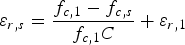 $$\varepsilon _{r{\comma }s} = \displaystyle{{f_{c{\rm\comma 1}} - f_{c{\comma s}} } \over {f_{c{\rm\comma 1}} C}} + \varepsilon _{r{\rm\comma 1}}$$
with
 $$C = \displaystyle{{f_{c{\rm\comma 1}} - f_{c{\rm\comma 2}} } \over {f_{{\rm c\comma 1}} \lpar \varepsilon _{r{\rm\comma 2}} - \varepsilon _{r{\rm\comma 1}} \rpar }} = \displaystyle{{\vint\!\!\!\vint\!\!\!\vint_{V_s } \varepsilon _0 {\bi E}_2 {\bi E}_1^\ast dV} \over {\vint\!\!\!\vint\!\!\!\vint_{V_{res} } \varepsilon \vert {\bi E}_1 \vert ^2 + \mu \vert {\bi H}_1 \vert ^2 dV}}.$$
The subscripts in equation (6) refer to the calibration materials 1 and 2, which were chosen as air and water in [Reference Haase and Jacob18]. V s and V res refer to the sample volume and the total resonator volume, respectively. ε 0 denotes the vacuum permittivity, ε and µ refer to the absolute permittivity and permeability. Ei and Hi represent the vectorial electric and magnetic fields in the resonator volume in the presence of the calibration material i (i = 1,2). The approach above assumes that the fields in the sampling volume are approximately equal for the sample and calibration material 2 (water). For this reason, the field integral in (6) can be substituted by a complex constant C.
In this work, the calibration is performed with air, water, and saline solutions. The accuracy of different sample pairs for the calibration is evaluated experimentally in Section V-B.
V. MEASUREMENTS
A) Measurement setup
The sensors are soldered to SMAconnectors and thus connected to an Agilent PNA E8361A two-port network analyzer. The network analyzer is calibrated at the plane of the connectors. The resonance is characterized using the transmission coefficient. The data are processed with Matlab.
The liquid samples are placed in the cylindrical reservoir described in Section II-D. The resonant frequencies of both sensors for the samples air and water, i.e., the empty reservoir and the reservoir filled with water, are listed in Table 3. Since an open structure is used in these measurements, the Q-factors include the radiation loss, which explains the differences compared to the values given in Table 2. The difference between the resonant frequency and the Q-factor for the two samples indicates the sensitivity of the sensor. It is clearly visible that Sensor 2 shows a higher sensitivity than Sensor 1 which corresponds to the findings in [Reference Haase and Jacob19].
Measured resonant frequency and Q-factor of the sensors for air and water samples without a shielding cover.

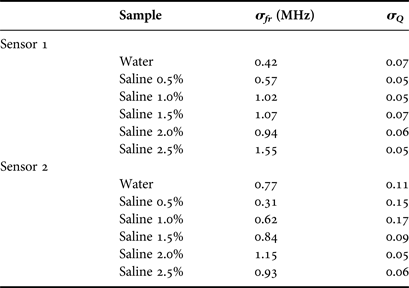
The liquids are filled into the reservoir several times and an average value is used for each liquid in order to minimize the errors caused by the network analyzer noise and by sample inhomogeneity. The standard deviations σ Q and σ fr for each sample are listed in Table 4. The uncertainty of the resonant frequency increases with the salt concentration. This is due to the lower Q, i.e. the broader resonance, leading to a stronger impact of the noise of the network analyzer. The resonant frequency and the Q-factor of Sensor 1 loaded with the liquid samples vary between 3.8 and 3.9 GHz and between 6 and 14, respectively. For Sensor 2, the resonant frequency lies between 4.5 and 4.6 GHz and the Q-factor between 12 and 22.
Standard deviations of measured resonant frequencies and quality factors.
B) Calibration validation
In order to validate the calibration method proposed above, a number of liquids with known permittivity are needed. Since well-characterized liquids with permittivities close to pure water are scarce, saline solutions of different concentrations are used. The solutions are prepared by weighing appropriate amounts of salt and water. The concentrations used in the experiments are 0.5 to 2.5% w/w.
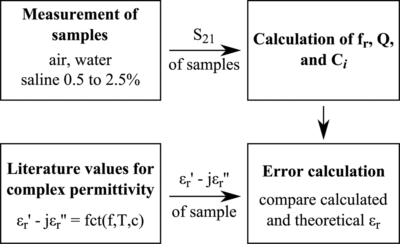
Three pairs of calibration liquids are compared in the following, i.e., air–water, water–saline 0.5%, and water–saline 1.5%. The calibrations resulting from the three sample pairs will be referred to as “cal 1”, “cal 2”, and “cal 3”, in the following. The data processing scheme used in the measurements is shown in Fig. 6.
Data evaluation of measured transmission coefficients.
The accuracy of the different calibration pairs is depicted in Fig. 7. The calculated permittivities are compared to the reference values from the literature [Reference Stogryn24].
Calculated permittivity of saline solutions with different calibration standards. Cal 1: air – water, cal 2: water–saline 0.5%, and cal 3: water–saline 1.5%. Reference values from [Reference Stogryn24]. (a) Sensor 1, real part of permittivity (b) Sensor 1, imaginary part of permittivity (c) Sensor 2, real part of permittivity, and (d) Sensor 2, imaginary part of permittivity.
Clearly, calibration pair 1 (air–water) shows the largest deviation from the reference values. Especially, the real part of the permittivity is not even a good estimate. Apparently, the interaction between the resonator and the sample is too strong for a linearization in the perturbation approach when using calibration materials with a high dielectric contrast. This stresses the necessity of adequate calibration materials, especially for Sensor 2.
For cal 2 and 3, the deviations are much lower as can be seen from the detailed plots in Fig. 8.
Real and imaginary parts of the difference between reference [24] and calculated permittivity for cal 2 and 3. (a) Sensor 1, and (b) Sensor 2.
Considering once more the perturbation approach, this is an expected improvement.
Previously, only one of the reference samples (water) was close to the permittivity of the samples (saline solutions). If one of the saline solutions is used instead of air, of course, the calculated complex constant C used for the calibration will be more suitable for the other saline solutions.
Overall, the accuracy is significantly improved when replacing the air calibration standard by a saline solution. However, the accuracy will only be acceptable in the vicinity of the permittivity of water, with the errors increasing with the contrast of the sample of interest compared to the calibration sample.
The improvement is most obvious for Sensor 2 since, because of the higher sensitivity, the cross-dependencies mentioned in Section II-C are stronger than those for Sensor 1. By using two calibration standards with a high permittivity and different loss tangents, the linearization inherent to the approach yields a better fit for samples with permittivities close to water. Of course, this is true for both sensors.
For aqueous solutions of low concentrations with permittivities close to deionized water and also for cell suspensions of low concentrations, the new calibration with two liquid standards instead of water and air is expected to lead to highly accurate results while using sensors of very high sensitivity.
VI. CONCLUSION
In this work, new variations of substrate-integrated near-field sensors are proposed. Two sensors based on circular half-mode sensors are analyzed in detail with respect to radiation. It is found that while the radiation is high for air as a sample (13–50%), it is strongly reduced for aqueous samples such as water and saline solutions (1–5%) and can thus be neglected. In addition, a calibration method for quantitative results is proposed and tested. It accounts for the complex dependence of the resonance on both permittivity and loss tangent of the sample under test. Compared to previous results, the accuracy for aqueous solutions of low concentrations is improved greatly by choosing suitable calibration materials.
Nora Meyne née Haase, received her Dipl.-Ing. degree in Electrical Engineering from the Technische Universität Hamburg-Harburg, Hamburg, Germany in 2011. She is currently working toward her Ph.D. at the Institut für Hochfrequenztechnik at the Technische Universität Hamburg-Harburg, Hamburg, Germany, in the field of electromagnetic interaction with biological tissues. Her research interests include the permittivity measurements of biological materials using resonant as well as broadband sensing devices.
Arne F. Jacob received the Dipl.-Ing. degree in Electrical Engineering in 1979 and the Dr.-Ing. degree in 1986 from the Technische Universität Braunschweig, Germany. From 1986 to 1988 he was a Fellow at CERN, the European Organization for Nuclear Research, Geneva, Switzerland. In 1988, he joined Lawrence Berkeley Laboratory, University of California at Berkeley for almost 3 years as a Staff Scientist at the Accelerator and Fusion Research Division. In 1990, he became a Professor at the Institut für Hochfrequenztechnik, Technische Universität Braunschweig. Since October 2004 he has been a Professor at the Technische Universität Hamburg-Harburg, Hamburg, Germany, where he heads the Institut für Hochfrequenztechnik. His current research interests include the design, packaging, and application of integrated (sub-)systems up to millimeter frequencies, and the characterization of complex materials.