



1. Introduction
The concept of vortex is of prime importance in revealing the underlying physics behind complex flows. In wall-bounded turbulence, the roles of vortices have been emphasized by extensive research works. In various self-sustaining mechanisms as reviewed by Panton (Reference Panton2001), quasi-streamwise vortices are closely linked to the low-speed streaks populated in the buffer layer (Hama Reference Hama1954; Kline et al. Reference Kline, Reynolds, Schraub and Runstadler1967), which is vital for the autonomous cycle of near-wall turbulence (Einstein & Li Reference Einstein and Li1958; Jiménez & Pinelli Reference Jiménez and Pinelli1999; Bandyopadhyay & Hellum Reference Bandyopadhyay and Hellum2014). On the other hand, investigation works focusing on the outer layer provide accumulated evidence that the hairpin vortices (Theodorsen Reference Theodorsen1952; Head & Bandyopadhyay Reference Head and Bandyopadhyay1981) and their well-organized packets (Adrian, Meinhart & Tomkins Reference Adrian, Meinhart and Tomkins2000) are the building blocks of large-scale motions.
A number of investigators are devoted to the study on the characteristics of vortices in wall-bounded turbulence. Usually, these vortices were recognized from velocity fields based on certain identification criteria (Chakraborty, Balachandar & Adrian Reference Chakraborty, Balachandar and Adrian2005). Tanahashi and his coworkers (Tanahashi et al. Reference Tanahashi, Kang, Miyamoto, Shiokawa and Miyauchi2004; Das et al. Reference Das, Tanahashi, Shoji and Miyauchi2006; Kang, Tanahashi & Miyauchi Reference Kang, Tanahashi and Miyauchi2007) extensively investigated the properties of the tube-like vortices (termed coherent fine-scale eddies, CFSEs) based on the direct numerical simulations (DNSs) of turbulent channel flows. When normalized by local Kolmogorov scale  $(\eta )$ and the root mean square of velocity fluctuations
 $({u_{rms}})$, the diameter and the maximum azimuthal velocity for CFSEs are 10–12η and 0.5–0.6urms respectively, independent of the wall-normal positions and Reynolds numbers (Das et al. Reference Das, Tanahashi, Shoji and Miyauchi2006). The universal scaling laws gained further supported by the DNS of turbulent channel flow at a higher friction Reynolds number
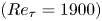 $(R{e_\tau } = 1900)$ (del Álamo et al. Reference del Álamo, Jiménez, Zandonade and Moser2006), and by the particle image velocimetry (PIV) of the turbulent boundary flows for
 $R{e_\tau }$ up to 6868 (Stanislas, Perret & Foucaut Reference Stanislas, Perret and Foucaut2008; Herpin et al. Reference Herpin, Stanislas, Jean and Coudert2013). Herpin et al. (Reference Herpin, Stanislas, Jean and Coudert2013) took into account for the orientation of vortices by conducting stereo PIVs in both the streamwise–wall-normal plane and the spanwise-wall-normal plane. They found that the probability density functions (p.d.f.s) of the vortex radius and the vorticity in the logarithmic layer can be fitted by a log-normal distribution in good qualities, and the fitting parameters show remarkably independent of Reynolds numbers.
Orientation is another aspect of vortex characteristics, which implies the elongating direction of vortex tubes and offers useful information to infer the topologies of dominant vortex structures. Ong & Wallace (Reference Ong and Wallace1998), Ganapathisubramani, Longmire & Marusic (Reference Ganapathisubramani, Longmire and Marusic2006) and Kang et al. (Reference Kang, Tanahashi and Miyauchi2007) inferred the vortex orientation based on the inclination angles of vorticity vectors. One widely cited result is that the vortex structures at the logarithmic layer tend to incline at an angle of 45° with respect to the streamwise direction, which was theoretically explained by Head & Bandyopadhyay (Reference Head and Bandyopadhyay1981). Bandyopadhyay (Reference Bandyopadhyay1980) conjectured that the upstream interface of large-scale motions consists of an array of 45°-inclined hairpin vortices with respect to the streamwise direction and derived the interface slope angle is 18.4°, consistent with the previous experimental observations. Against the use of vorticity direction as the vortex orientation, Bernard, Thomas & Handler (Reference Bernard, Thomas and Handler1993) and Gao, Ortiz-Dueñas & Longmire (Reference Gao, Ortiz-Dueñas and Longmire2007) argued that the local vorticity vector tends to be deflected away from the vortex axis at locations very close to the wall. Zhou (Reference Zhou1997) demonstrated that the real eigenvector  $({\boldsymbol{\varLambda }_r})$ of the velocity gradient tensor is well aligned with the vortex axis by tracking
 ${\boldsymbol{\varLambda }_r}$ within a hairpin vortex. Using
 ${\boldsymbol{\varLambda }_r}$ as the indicator for vortex orientation, Gao, Ortiz-Dueñas & Longmire (Reference Gao, Ortiz-Dueñas and Longmire2011) refined the vortex characteristics including orientations, circulation, propagation velocities at three different wall-parallel planes. Recently, Tian et al. (Reference Tian, Gao, Dong and Liu2018) proposed a new definition for the orientation of vortex based on the coordinate transformation, which turned out to be
 ${\boldsymbol{\varLambda }_r}$ (Gao & Liu Reference Gao and Liu2018). Also based on
 ${\boldsymbol{\varLambda }_r}$ criterion, Wang et al. (Reference Wang, Gao, Wang, Wang and Pan2019) extended the work of Gao et al. (Reference Gao, Ortiz-Dueñas and Longmire2011) and offered full information of vortex orientation, shapes and organizations for larger Reynolds-number range
 $(R{e_\tau } = 1238 \sim 3081)$ based on tomographic PIV data and DNS data.
Besides aforementioned works regarding general vortices, there are also a lot of investigations focusing on the vortices with specific geometries for the modelling purpose, such as the hairpin vortices, packets or attached vortex structures. Christensen & Adrian (Reference Christensen and Adrian2001) statistically investigated the geometrical characteristics of packets structures in the streamwise–wall-normal plane, and found their streamwise inclination angle with respect to the wall is 12°–13°. Wu & Christensen (Reference Wu and Christensen2006) investigated the population trends of prograde and retrograde spanwise vortices in wall turbulence. Natrajan, Wu & Christensen (Reference Natrajan, Wu and Christensen2007) recognized the pairing trend of prograde and retrograde vortices and interpreted the vortex pairing as the signature of a  $\varOmega $-shape vortex. Deng et al. (Reference Deng, Pan, Wang and He2018) filtered out the spanwise vortices not aligned in a packet based on proper orthogonal decomposition and discovered a
 $Re_\tau ^{1/2}$ scaling of the saturated streamwise spacing between two hairpin heads in one packet. Besides these PIV measurements limited in the streamwise–wall-normal plane, Ganapathisubramani, Longmire & Marusic (Reference Ganapathisubramani, Longmire and Marusic2003) recognized the patterns of vortex packets in the streamwise–spanwise plane and estimated that these patterns contribute more than 25 % to the total Reynolds stress while occupying only 5 % of the total area in the logarithmic layer. Hutchins, Hambleton & Marusic (Reference Hutchins, Hambleton and Marusic2005) investigated the patterns of hairpin packets in the 135°-inclined plane with respect to the streamwise direction and found distinct two-regime behaviours: attached to the wall and detached from it, with a demarcation scaled well with the outer variables. The attached and detached structures were also reported by del Álamo et al. (Reference del Álamo, Jiménez, Zandonade and Moser2006), who recognized tall attached vortex clusters and detached vortex clusters based on three-dimensional (3-D) DNS data of turbulent channel flow. They found that the attached eddies are self-similar with a constant height–width–length of 1 : 1.5 : 3 while the sizes of detached eddies are proportional to the local Kolmogorov scale.
These investigations involve the statistical information about the size, intensity, orientation and organizations of vortices in wall-bounded turbulence, which add to the understanding of the wall-turbulence structures and also provide valuable materials for the modelling works. The hairpin model and the attached eddy model are two well-known models in the wall-turbulence community. The hairpin model, first proposed by Theodorsen (Reference Theodorsen1952), gained renewed interest after the experimental investigations of Bandyopadhyay (Reference Bandyopadhyay1980) and Head & Bandyopadhyay (Reference Head and Bandyopadhyay1981). Adrian (Reference Adrian2007) extended the hairpin model by invoking the packet features found by PIV, and put forward a conceptual multi-hairpin paradigm to explain many observations in wall turbulence. The attached eddy model was proposed by Townsend (Reference Townsend1956), which provided a theoretical framework to predict the flow statistics in the logarithmic region. Perry and his coworkers (Perry & Chong Reference Perry and Chong1982; Perry, Henbest & Chong Reference Perry, Henbest and Chong1986; Marusic & Perry Reference Marusic and Perry1995; Perry & Marusic Reference Perry and Marusic1995) advanced the attached eddy model by using a hairpin-shape vortex skeleton as the attached eddy candidate, and gave a recipe for inferring the turbulence intensity distributions and the turbulence spectra. More recently, the attached eddy theory has achieved vast success in predicting the statistics (Woodcock & Marusic Reference Woodcock and Marusic2015; Yang, Marusic & Meneveau Reference Yang, Marusic and Meneveau2016) and in recovering the instantaneous flow features, including the uniform momentum zone (de Silva, Hutchins & Marusic Reference de Silva, Hutchins and Marusic2016a) and large coherence structures of spanwise velocities (de Silva et al. Reference de Silva, Kevin, Baidya, Hutchins and Marusic2018). Marusic & Monty (Reference Marusic and Monty2019) reviewed the past research works and discussed underlying assumptions for the attached eddy model.
The hairpin model and the attached eddy model share the same notion that the chaotic and multiscale wall turbulence can be represented by a collection of more elementary structures. These elementary structures could be typical vortex models obtained by averaging many instantaneous vortex structures in wall turbulence. These aforementioned investigations regarding vortex characteristics provide references for refining the geometry of the vortex model. Once the vortex geometry is specified, a translation from vortex to velocity is necessary, which is termed as the vortex-to-velocity (V2V) reconstruction in the present work. Perry & Marusic (Reference Perry and Marusic1995) formulated a Gaussian distribution of vorticity in the vortex cores, with the vorticity orientation consistent with the vortex axis. Subsequently, they employed the well-known Biot–Savart law to reconstruct the velocity field in the logarithmic region. It was assumed that the vorticity is concentrated inside the vortex cores and the surrounding flows could be regarded as irrotational (Perry & Chong Reference Perry and Chong1982). Nevertheless, for the buffer layer, the surrounding vorticity cannot be neglected due to the stronger viscosity effect. Besides, the vorticity direction could also deviate from the vortex orientation (Wang et al. Reference Wang, Gao, Wang, Wang and Pan2019). Extending application range for the vortex model to the buffer region will pose new challenges for the V2V reconstruction, which necessitates new methods in place of the Biot–Savart law.
Besides the velocity reconstruction based on ideal vortex models, the reconstruction based on real instantaneous vortex fields is also beneficial for the analysis regarding the inducing effects of vortices in wall turbulence. In the investigation of Ganapathisubramani et al. (Reference Ganapathisubramani, Longmire and Marusic2003), the contribution of vortex packets to the Reynolds shear stress was estimated based on a pattern-recognized strategy. Specifically, only the low-speed streaks flanked by packets were counted in the contribution, which caused an underestimated result because the packets also induce the sweep events (high-speed zones) besides the low-speed streaks (Marusic & Adrian Reference Marusic and Adrian2012). Recently, Berk & Ganapathisubramani (Reference Berk and Ganapathisubramani2019) employed the Biot–Savart law to derive the vortex-induced velocity when dealing with a synthetic jet issuing into a turbulent boundary layer, which highlighted the including effects of vortices. A more correlated work on canonical wall turbulence is reported by Pirozzoli, Bernardini & Grasso (Reference Pirozzoli, Bernardini and Grasso2010), who compared the roles of vortex tubes and vorticity sheets (termed as vortex sheets in their article) by separately reconstructing velocity fields based on these two types of structures. A Poisson equation was solved to implement the reconstruction, which had been developed for the reconstruction regarding the intense vorticity (Jiménez et al. Reference Jiménez, Wray, Saffman and Rogallo1993). The reconstructed results based on only vortex tubes are not very organized, especially at the buffer layer compared with the results of vortex sheets. They concluded that the vorticity sheets had a more important collective effect and contributed more to the turbulence production. However, it should be pointed out that the effects of vortex tubes might be underestimated since the reconstruction method was established for the vorticity-based reconstruction.
A generalized discussion on how to reconstruct velocity fields based on given vortex fields also builds on the well-developed vortex identification methods, which remains a focus in the turbulence community up to the present day (Tian et al. Reference Tian, Gao, Dong and Liu2018; Xiong & Yang Reference Xiong and Yang2019; Zhu & Xi Reference Zhu and Xi2019). The starting point of various vortex identification schemes is to extract tube-like vortices from complex flows, removing the influence of the surrounding shear layers in the flow. The vortex tubes are quite sparse in the spatial field and could be simply represented as 3-D curved lines with fewer adjustable parameters. The process of extracting vortices from turbulence is much like a data compression process, as pointed out by Chakraborty et al. (Reference Chakraborty, Balachandar and Adrian2005). V2V reconstruction is the inverse process of this compression, which decompresses the vortex representations to recover original turbulence fields. Naturally, the compression and decompression are two fundamental aspects for the vortex-representing principle of wall-bounded turbulence, yet only the former has been focused on in the previous investigations.
Motivated by these considerations, the current work will focus on the topic of the V2V reconstruction. It should be addressed that the current work mainly considers the kinematic representation of wall turbulence. The current V2V reconstruction is also different from the vorticity-based velocity reconstruction involved in the vortex method for simulating the Navier–Stokes equations (Leonard Reference Leonard1985; Koumoutsakos & Leonard Reference Koumoutsakos and Leonard1995; Bernard Reference Bernard2013; Caprace, Winckelmans & Chatelain Reference Caprace, Winckelmans and Chatelain2020). In those works, the velocity field is reconstructed based on the vorticity field. Basically, the intense-vorticity regions could take the forms of filaments, sheets and blobs, yet only the filament (or tube-like) elements are recognized as vortices for most situations (Marusic & Adrian Reference Marusic and Adrian2012). The current work focuses on tubular vortices and regards them as the constructing elements of wall turbulence, which is the common spirit of many structure-based models. Perry & Chong (Reference Perry and Chong1987) commented that ‘these vortex skeletons are the “genetic code” of the flow field, since this requires very little specification and the Biot-Savart law can be used to generate the velocity field’. Thus, we confine that the reconstruction in the current investigation should use the geometry and strength information of tubular vortices only. For convenience, a vortex field will be defined by combining the existing identification criteria for the vortex magnitude and orientation, which contain all the information required for the reconstruction.
In this work, the V2V reconstruction will be implemented by a data-driven method, termed field-based linear stochastic estimation, which is a generalized method to estimate one 3-D field based on another. Mathematically, the new method could be viewed as the least-square estimation on the linear inducing effects of vortices. The reconstruction accuracy will be estimated and compared with the Biot–Savart law. Before introducing the V2V reconstruction, the geometrical property of the vortex field will be investigated, with the purpose of showing the distinct aspect differing from the vorticity field. An interesting aspect about the relationship between vortex magnitude and orientation will be revealed based on the differential geometry, which supports the definition of the vortex vector.
The remainder of this work is arranged as follows. In § 2, the DNS data employed in this investigation and associated numerical processing techniques are introduced. In § 3, the geometrical property of the vortex field is discussed. Subsequently, the theory and implementation for the field-based linear stochastic estimation as a V2V reconstruction method are introduced in § 4. In § 5, the V2V reconstruction method is numerically validated and compared with the Biot–Savart law. The inducing effects of vortices, the limitations of the method and the roles of strong and weak vortex components are further discussed based on the reconstruction results, followed by the concluding remarks in § 6.
2. The DNS data and processing techniques
2.1. The DNS data
The data employed by this work came from an open-access DNS database (https://torroja.dmt.upm.es/) for high-Reynolds-number turbulent boundary layer (TBL). A full description of the algorithm and the computational set-up could be found in the papers of Simens et al. (Reference Simens, Jiménez, Hoyas and Mizuno2009) and Borrell, Sillero & Jiménez (Reference Borrell, Sillero and Jiménez2013). Basically, their simulation bypassed the transition stage for boundary layer and directly generated a developed TBL with accurate inflow conditions. The inflow for this simulation was fed by an auxiliary simulation, whose calculation domain is located at the upstream of the main simulation domain. The inflow for the auxiliary simulation was obtained from one plane in its own domain using a rescaling–recycling scheme (Lund, Wu & Squires Reference Lund, Wu and Squires1998).
The DNS data (Sillero, Jiménez & Moser Reference Sillero, Jiménez and Moser2013) have been widely validated by the Jiménez group (Borrell et al. Reference Borrell, Sillero and Jiménez2013; Sillero et al. Reference Sillero, Jiménez and Moser2013; Sillero, Jiménez & Moser Reference Sillero, Jiménez and Moser2014). Particularly, Sillero et al. (Reference Sillero, Jiménez and Moser2013) showed that the skin friction and shape factor from this simulation agree well with the empirical fit of Monkewitz, Chauhan & Nagib (Reference Monkewitz, Chauhan and Nagib2007), with the mean percentage deviations less than 1 %. This indicates that the canonical asymptotic state is attained after the relaxation of the auxiliary simulation. A number of investigators (Marusic, Baars & Hutchins Reference Marusic, Baars and Hutchins2017; Wang, Wang & He Reference Wang, Wang and He2017; Wang et al. Reference Wang, Pan, Gao and Wang2018; Chen & Sreenivasan Reference Chen and Sreenivasan2021; Wang, Pan & Wang Reference Wang, Pan and Wang2021) cited the DNS dataset in their investigation works. In our previous work (Wang et al. Reference Wang, Gao, Wang, Wang and Pan2019), we compared the DNS data with 3-D PIV data regarding several aspects, including the p.d.f. of the vortex orientation angles and the conditionally averaged vortex structures. The DNS results and the experimental results were remarkably consistent, which further emboldens us to use the DNS data.
The production DNS field corresponds to a spatially evolving zero pressure gradient TBL from  $R{e_\tau } \approx \textrm{1000}$ to
 $R{e_\tau } \approx \textrm{2000}$. The calculation domain contains 15361, 4096 and 535 grid nodes for the streamwise, spanwise and wall-normal directions, respectively. The separation between adjacent collocation points along the wall-normal direction is non-uniform, which is determined by local Kolmogorov scale (Borrell et al. Reference Borrell, Sillero and Jiménez2013). The DNS dataset is fully resolved and covers a vast scale range, which provides an ideal database for the implementation and validation of the V2V reconstruction.
In this work, only the data segments for  $R{e_\tau } = 1148 \sim 1250$ were truncated from the whole DNS field. The average boundary thickness, determined by the height with 99 % of the free stream velocity, is approximately 1200 wall units, i.e.
 $\delta^{+} \approx 1200$. The selection for this boundary thickness was based on two considerations. From the perspective of the V2V reconstruction, the logarithmic layer of this data segment covers a wall-normal range of approximately 160 wall units (from 80 wall units to
 $0.2\delta^{+}$), corresponding to an acceptable number of computational nodes for the V2V reconstruction. On the other hand, investigations (Tanahashi et al. Reference Tanahashi, Kang, Miyamoto, Shiokawa and Miyauchi2004; del Álamo et al. Reference del Álamo, Jiménez, Zandonade and Moser2006; Herpin et al. Reference Herpin, Stanislas, Jean and Coudert2013; Wang et al. Reference Wang, Gao, Wang, Wang and Pan2019) have validated that the fine-scale vortices populated in TBL present universal behaviours, independent of the Reynolds number. The truncated DNS data segment has a streamwise dimension of
 $8\delta^{+}$, a spanwise dimension of
 $13.4\delta^{+}$, and a wall-normal range from the viscous sublayer to
 $\textrm{0}\textrm{.3}\delta^{+}$, corresponding to a Cartesian grid of
 $1412 \times 4096 \times 91$. The variation range of the viscous wall unit in the DNS data segments is ±0.8 %, which is small enough to be viewed as a constant. Totally, twelve frames of DNS fields were downloaded, providing sufficient data for deriving the statistical quantities. To minimize the processing errors, all the calculations in the present work were based on the original DNS grid. The derivative computations were performed via a 5-node central differential scheme. More parameters about the DNS data segments employed in this work are collected in table 1.
A collection of parameters for the DNS data employed in this work.

Throughout this article, the coordinate origin is located on the wall, and  $x,y,z$ align with the streamwise, spanwise and wall-normal directions, respectively. The variable t indicates the time dimension.
 $\boldsymbol{u}$ denotes the fluctuating velocity vector, obtained by subtracting the mean streamwise velocity component from the original DNS vector field;
 $u,v,w$ designate the streamwise, spanwise and wall-normal fluctuating velocity components, respectively. A superscript of ‘+’ indicates that the quantity is normalized by the wall unit or the friction velocity. Only the fluctuating velocity field is considered in the following analysis.
2.2. The vortex identification
Various vortex identification criteria were developed to extract filamentary (tube-like) vortices from turbulence. Most of them are based on local velocity gradient tensor ( $\boldsymbol{\nabla }\boldsymbol{u}$), including the second invariant Q (Hunt, Wray & Moin Reference Hunt, Wray and Moin1988), the discriminant
 $\varDelta$ (Chong, Perry & Cantwell Reference Chong, Perry and Cantwell1990), the swirl strength
 ${\lambda _{ci}}$ (Zhou et al. Reference Zhou, Adrian, Balachandar and Kendall1999), the
 ${\lambda _2}$ criterion (Jeong & Hussain Reference Jeong and Hussain1995) and so on. Commonly, the iso-surfaces of the criterion for one prescribed value are displayed as recognized vortices. Chakraborty et al. (Reference Chakraborty, Balachandar and Adrian2005) revealed the relationships between these identification criteria and demonstrated that results from different criteria are approximately equivalent for turbulent flows. Among these criteria, the swirl strength
 $({\lambda _{ci}})$ corresponds to the imaginary part of the complex eigenvalue of the velocity gradient tensor, which has the same dimension as vorticity. A lot of investigators (Ganapathisubramani et al. Reference Ganapathisubramani, Longmire and Marusic2006; Hambleton, Hutchins & Marusic Reference Hambleton, Hutchins and Marusic2006; Lee & Sung Reference Lee and Sung2009) used ‘signed swirl’ as the representative variable for the in-plane component of a vortex, which is obtained by multiplying
 ${\lambda _{ci}}$ by the sign of the out-of-plane component of vorticity. For eduction purposes, Pirozzoli et al. (Reference Pirozzoli, Bernardini and Grasso2010) defined the strength of vortex tubes by introducing a ‘vorticity-like’ variable, which is equal to
 $2{\lambda _{ci}}$.
As for the vortex orientation, Gao et al. (Reference Gao, Ortiz-Dueñas and Longmire2011) and Tian et al. (Reference Tian, Gao, Dong and Liu2018) suggested using the real eigenvector of  $\boldsymbol{\nabla }\boldsymbol{u}$ (denoted as
 ${\boldsymbol{\varLambda }_r}$). Tian et al. (Reference Tian, Gao, Dong and Liu2018) gave a mathematical discussion on the definition of the vortex vector based on the Schur decomposition theory (Gentle Reference Gentle1998). According to the viewpoint of Tian et al. (Reference Tian, Gao, Dong and Liu2018), the vortex orientation
 $({\boldsymbol{\varLambda }_r})$ corresponds to a direction with zero rotation speed. As indicated by the definition of velocity gradient tensor
 $(\boldsymbol{\nabla }\boldsymbol{u})$, the relative velocity
 $\delta \boldsymbol{u}$ for two points separated by a small position vector
 $\delta \boldsymbol{r}$ could be expressed as
 \begin{equation}\delta \boldsymbol{u} = \boldsymbol{\nabla }\boldsymbol{u}\boldsymbol{\cdot }\delta \boldsymbol{r}.\end{equation}
The non-rotation requirement means that the relative velocity should be along  $\delta \boldsymbol{r}$, which means
 \begin{equation}\boldsymbol{\nabla }\boldsymbol{u}\boldsymbol{\cdot }\delta \boldsymbol{r} = \mu \delta \boldsymbol{r},\end{equation}
where  $\mu $ should be a real constant. The above equation implies that
 $\delta \boldsymbol{r}$ is the real eigenvector of
 $\boldsymbol{\nabla }\boldsymbol{u}$, viz.
 ${\boldsymbol{\varLambda }_r}$.
Considering the eigenvector  $({\boldsymbol{\varLambda }_r})$ contains no sign information about rotation, the local vorticity
 $\boldsymbol{\omega }$ is used as a reference. Specifically, the eigendirection (
 ${\boldsymbol{\varLambda }_r}$ or
 $- {\boldsymbol{\varLambda }_r}$) forming an acute included angle with
 $\boldsymbol{\omega }$ is viewed as the vortex orientation. In this work, for the convenience of numerical implementation, the swirl strength
 ${\lambda _{ci}}$ and the orientation vector
 ${\boldsymbol{\varLambda }_r}$ are combined to define a vector field as
 \begin{equation}\boldsymbol{\varLambda } = {\lambda _{ci}}\textrm{sign}({\boldsymbol{\varLambda }_r}\boldsymbol{\cdot }\boldsymbol{\omega }){\boldsymbol{\varLambda }_r},\end{equation}
where ‘sign’ is the sign function, returning the sign of the bracketed variable. Throughout this article, the vortex field refers to  $\boldsymbol{\varLambda }$ as default, which is consistent with the definition by Wang et al. (Reference Wang, Gao, Wang, Wang and Pan2019). It should be remembered that (2.3) is not a widely accepted expression since no mathematical definition for a vortex is available so far. In this work, the vortex field serves as a carrier for the geometrical and strength information of tubular vortices, which is necessary for the V2V reconstruction. In the following § 3, we will inspect the definition of (2.3) from the respect of the geometrical property of the recognized vortices.
2.3. The correlation coefficient and the complex coherence spectrum
A successful V2V reconstruction should return a velocity field sharing a high degree of similarity with the original DNS field, which can be measured by the correlation coefficient (CC). The CC is an indicator of the linear correlation degree between two input signals. In the current investigation, the CC for the reconstructed/original streamwise velocity components at one wall-normal position  $({z_0})$ is calculated by
 \begin{equation}CC({z_0}) = \frac{{{{\langle {u_{rec}}(x,y,{z_0},t){u_{DNS}}(x,y,{z_0},t)\rangle }_{x,y,t}}}}{{\sqrt {{{\langle {u_{rec}}{{(x,y,{z_0},t)}^2}\rangle }_{x,y,t}}{{\langle {u_{DNS}}{{(x,y,{z_0},t)}^2}\rangle }_{x,y,t}}} }}.\end{equation}
Herein,  ${u_{rec}}(x,y,z,t)$ and
 ${u_{DNS}}(x,y,z,t)$ denote the reconstructed streamwise velocity component field and the corresponding DNS field;
 ${\langle \cdot \rangle _{x,y,t}}$ represents the ensemble average, which is implemented by averaging the quantities in the brackets along the homogeneous dimensions, including the temporal dimension (t) and the wall-parallel dimensions (x and y), as indicated by the subscript
 $x,y,t$. The CCs regarding other velocity components (v and w) are calculated based on similar expressions with (2.4).
As a refined variant for CC, the complex coherence spectrum (CCS) measures the scale-specific linear coherence of two input signals (Stoica & Moses Reference Stoica and Moses2005; Ramirez, Via & Santamaria Reference Ramirez, Via and Santamaria2008). In the current work, the CCS formula takes a form resembling the correlation coefficient, but in the spectral representation. Specifically, the streamwise CCS between  ${u_{rec}}(x,y,z,t)$ and
 ${u_{DNS}}(x,y,z,t)$ at a given wall-normal position
 $({z_0})$ could be calculated by
 \begin{align}CCS(k\textrm{)} = \frac{{{{\langle {{\tilde{u}}_{rec}}(k,y,{z_0},t){{\tilde{u}}_{DNS}}{{(k,y,{z_0},t)}^\ast }\rangle }_{y,t}}}}{{\sqrt {{{\langle {{\tilde{u}}_{rec}}(k,y,{z_0},t){{\tilde{u}}_{rec}}{{(k,y,{z_0},t)}^\ast }\rangle }_{y,t}}{{\langle {{\tilde{u}}_{DNS}}(k,y,{z_0},t){{\tilde{u}}_{DNS}}{{(k,y,{z_0},t)}^\ast }\rangle }_{y,t}}} }}.\end{align}
In (2.5),  ${\tilde{u}_{rec}}(k,y,{z_0},t)$ and
 ${\tilde{u}_{DNS}}(k,y,{z_0},t)$ denotes the streamwise (1-D) Fourier-transform coefficient of
 ${u_{rec}}(x,y,z,t)$ and
 ${u_{DNS}}(x,y,z,t)$, respectively; k denotes the corresponding wavenumber. For convenience,
 ${\tilde{u}_{rec}}(k,y,{z_0},t)$ and
 ${\tilde{u}_{DNS}}(k,y,{z_0},t)$ are simply represented by
 ${\tilde{u}_{rec}}(k)$ and
 ${\tilde{u}_{DNS}}(k)$ in the following discussions. Notably, both
 ${\tilde{u}_{rec}}(k)$ and
 ${\tilde{u}_{DNS}}(k)$ are complex numbers, carrying the scale-specific amplitude and phase information of the input velocity fields. The asterisk designates the complex conjugate operation;
 ${\langle \cdot \rangle _{y,t}}$ indicates averaging the quantities in the brackets along the temporal dimension and the spanwise direction, which is simply denoted as
 $\langle \cdot \rangle$ in the following discussions. Equation (2.5) results in a complex number, which is different from the linear coherence spectrum (LCS) used by Baars & Marusic (Reference Baars and Marusic2020a). In their work, the LCS was defined as the squared magnitude of the current CCS, which measures the scale-by-scale coupling degree for two-point velocity signals. The phase angle of the CCS indicates the scale-by-scale phase deviation, which is also considered as the indicator for accessing the V2V reconstruction.
To illuminate the physical implication of (2.5), we express  ${\tilde{u}_{rec}}(k)$ and
 ${\tilde{u}_{DNS}}(k)$ by the exponential forms, viz.
 ${\tilde{u}_{rec}}(k)\textrm{ = }{A_{rec}}(k)\,{\textrm{e}^{\textrm{i}{\gamma _{rec}}(k)}}$ and
 ${\tilde{u}_{DNS}}(k)\textrm{ = }{A_{DNS}}(k)\,{\textrm{e}^{\textrm{i}{\gamma _{DNS}}(k)}}$. Herein,
 ${A_{rec}}(k)$ and
 ${A_{DNS}}(k)$ stand for the amplitudes of
 ${\tilde{u}_{rec}}(k)$ and
 ${\tilde{u}_{DNS}}(k)$, respectively;
 ${\gamma _{rec}}(k)$ and
 ${\gamma _{DNS}}(k)$ indicate the corresponding phase angles. By substituting
 ${\tilde{u}_{rec}}(k)$ and
 ${\tilde{u}_{DNS}}(k)$ in (2.5) with their exponential forms, it could be easily derived that
 \begin{equation}CCS(k) = \langle {\hat{A}_{rec}}(k){\hat{A}_{DNS}}(k)\,{\textrm{e}^{\textrm{i}\Delta \gamma (k)}}\rangle .\end{equation}
In (2.6),  ${\hat{A}_{rec}}(k) = {{{A_{rec}}(k)} / {\sqrt {\langle {A_{rec}}{{(k)}^2}\rangle } }}$ and
 ${\hat{A}_{DNS}}(k) = {{{A_{DNS}}(k)} / {\sqrt {\langle {A_{DNS}}{{(k)}^2}\rangle } }}$, which could be viewed as the normalized amplitudes;
 $\Delta \gamma (k) = {\gamma _{rec}}(k) - {\gamma _{DNS}}(k)$ represents the phase deviation between
 ${\tilde{u}_{rec}}(k)$ and
 ${\tilde{u}_{DNS}}(k)$;
 ${\textrm{e}^{\textrm{i}\Delta \gamma (k)}}$ is the polar representation for the phase deviation
 $\Delta \gamma (k)$. Equation (2.6) means that the CCS equals the weighted average of the sample data for
 ${\textrm{e}^{\textrm{i}\Delta \gamma (k)}}$, and the corresponding weighting coefficients are
 ${\hat{A}_{rec}}(k){\hat{A}_{DNS}}(k)$.
For the sake of clarity, we first disregard the weighting coefficient and consider the special case of  $LCS(k) = \langle {\textrm{e}^{\textrm{i}\Delta \gamma (k)}}\rangle$. In this case, the CCS is determined by the phase deviation between
 ${\tilde{u}_{rec}}(k)$ and
 ${\tilde{u}_{DNS}}(k)$. If
 ${\tilde{u}_{rec}}(k)$ and
 ${\tilde{u}_{DNS}}(k)$ are extremely incoherent in phase, their phase deviation, deemed as a random variable, would present a uniform probability distribution between 0 and 2
 ${\rm \pi}$. In the complex coordinate system (as shown by figure 1a), the samples of
 ${\textrm{e}^{\textrm{i}\Delta \gamma (k)}}$ (blue circles) would be spread evenly on the unit circle around the origin. Thus, the centre of these scattered numbers (i.e. the statistical average, CCS) would occur very close to the origin. On the contrary, if the
 ${\tilde{u}_{rec}}(k)$ and
 ${\tilde{u}_{DNS}}(k)$ are coupled in phase, these hollow circles would cluster towards one specific orientation (as shown in figure 1b). The central point (the red dot) would be in close proximity to the unit circle, giving a CCS with a magnitude close to one. The above explanation can be extended to the general cases of (2.6), as long as these scattered sampling points are given different weighting coefficients when calculating the central point. In this sense, the CCS incorporates both the phase and magnitude information from
 ${\tilde{u}_{rec}}(k)$ and
 ${\tilde{u}_{DNS}}(k)$, and provides a comprehensive diagnosis on their scale-specific coherence relation.
Schematic plots for illustrating the relation between CCS and the distribution of the phase deviations  $(\Delta \gamma )$ for a set of input signal samples. The sample data of
 ${\textrm{e}^{\textrm{i}\Delta \gamma }}$ are schematically displayed in the complex coordinate system by hollow blue circles. The red dot, which is the centre of the blue circles, marks the position of CCS (
 $CCS\textrm{(}k) = \langle {\textrm{e}^{\textrm{i}\Delta \gamma }}\rangle$). Panel (a) corresponds to the situation with a small CCS magnitude; (b) corresponds to the situation with a large CCS magnitude.

3. The geometrical property of the vortex field
As the cornerstone of the V2V reconstruction, the vortex field defined in § 2.2 merits a special discussion. This section will focus on the geometrical property of the vortex field. To start this discussion, an observation on the instantaneous field is beneficial. Figure 2 shows the structures identified by iso-surfaces of vorticity magnitude  $(\omega )$ and vortex intensity
 $({\lambda _{ci}})$, with orientation vectors displayed on the surfaces. For a clear display, only the iso-surfaces for
 ${z^ + } \le 120$ are shown in the figure. Since both
 $\omega $ and
 ${\lambda _{ci}}$ are calculated based on the fluctuating velocity field, the influence of mean shear in TBL has been removed. The thresholds for
 $\omega $ and
 ${\lambda _{ci}}$ are prescribed so that the identified structures occupy approximately 10 % of the total volume displayed. Distinct characteristics for the
 $\omega $-identified and
 ${\lambda _{ci}}$-identified structures are noticed. The former contains large bulks of flat sheet-like entities at the lower layer and thin tube-like entities above. The latter recognizes only the vortex tubes with a thickness of about ten wall units. In figure 2(b), several vortex tubes incline at an angle of approximately 45° with respect to the streamwise direction, which is similar to the criss-cross patterns observed by Bandyopadhyay (Reference Bandyopadhyay and Perry1989) in the laser-light-sheet smoke flow visualization pictures. While a typical hairpin vortex is not observed, there are some vortex tubes resembling twisted single-leg hairpin vortices. Mostly, the vortex vectors are attached in the vortex surface and pointing to the extending direction of the vortex tubes. This property has also been reported by Tian et al. (Reference Tian, Gao, Dong and Liu2018), who regarded it as a support for their definition of vortex orientation. For the vorticity field, the property does not hold at the near-wall region, where the vorticities tend to be aligned with the spanwise direction. A correlated work involving this property is reported by Xiong & Yang (Reference Xiong and Yang2019), who attempted to calculate the ‘vorticity surface field’ based on the vorticity field. A scalar field is called the vorticity surface field if the normal vector of its iso-surface is perpendicular to the local vorticity vector. If this concept is used for the present vortex field, we can see that
 ${\lambda _{ci}}$ could be approximately regarded as the ‘vortex surface field’.
Instantaneous flow structures identified by vorticity magnitude (a) and vortex magnitude (b). The surfaces in the two plots correspond to  ${\omega ^ + } = 0.4\textrm{2}$ and
 $\lambda _{ci}^ +{=} 0.10$ respectively, coloured based on the distance from the wall. Orientations of vorticity and vortex on the surfaces are also displayed by red vectors. For clarity, only one in four vectors in each direction are shown.

To quantitatively analyse the relationship between the vortex surface and the vortex orientation, we resort to the differential geometry, which is a useful mathematical tool to describe the local curvatures of a surface. Consider a small vortex surface element S as shown in figure 3(a), which can be viewed as a quadratic surface;  $\boldsymbol{n}$ denotes the normal vector of S, pointing to the side with smaller vortex magnitude. Generally, two orthogonal principal directions (indicated by two unite vectors:
 ${\boldsymbol{\kappa }_1}$ and
 ${\boldsymbol{\kappa }_2}$) can be determined on S, which correspond to the directions with the maximum and minimum curvatures, respectively;
 ${\boldsymbol{\kappa }_1}$ and
 ${\boldsymbol{\kappa }_2}$ refer to the first principal direction and the second principal direction for the local curvatures. Taking an example of a straight vortex tube with a uniform radius (see figure 3b), the two principal directions (
 ${\boldsymbol{\kappa }_\textrm{1}}$ and
 ${\boldsymbol{\kappa }_2}$) are aligned with the axial direction and azimuthal direction, respectively. The corresponding curvatures for
 ${\boldsymbol{\kappa }_\textrm{1}}$ and
 ${\boldsymbol{\kappa }_2}$ refer to the local curvatures of lines extracted along the two directions from the surface (see
 ${l_1}$ and
 ${l_2}$ in figure 3b), which are 0 and
 $- 1/R$ respectively. The negative sign indicates that the extracted line
 $({l_2})$ bends toward the negative direction of
 $\boldsymbol{n}$. Thus, we can see that the vortex orientation is aligned with
 ${\boldsymbol{\kappa }_\textrm{1}}$ for a straight vortex tube. For general thin and tube-like vortices, one can guess that the vortex orientation also tends to align with
 ${\boldsymbol{\kappa }_\textrm{1}}$, which will be tested and verified in the following discussion.
Diagrammatic sketches for the principal directions of the local curvatures.

For each point in the vortex field, the vortex surface passing this point could be extracted, and correspondingly the normal vector  $\boldsymbol{n}$ and the principal directions (
 ${\boldsymbol{\kappa }_\textrm{1}}$ and
 ${\boldsymbol{\kappa }_2}$) can be determined. Detailed introduction for this process is provided in Appendix A of this article;
 ${\boldsymbol{\kappa }_\textrm{1}}$,
 ${\boldsymbol{\kappa }_2}$ and
 $\boldsymbol{n}$ constitute a local coordinate system, and we can investigate the vortex orientation in this local coordinate system. Specifically, a transformation from the global coordinate system to this local coordinate system is performed on the vortex vector. Subsequently, in the local coordinate system, the vortex vector is further expressed by three spherical coordinates: radical distance
 $(\rho )$, azimuth angle
 $(\psi )$ and zenith angle
 $(\theta )$. The joint p.d.f. of
 $\psi$ and
 $\theta$ is calculated based on the data points with
 $\lambda _{ci}^ + > 0.1\textrm{0}$ and
 ${z^ + } \le 0.3{\delta ^ + }$. The threshold, which is consistent with the one used in figure 2, is deployed here to exclude the influence of weak vortices. The resulting p.d.f. is further normalized by
 $\sin (\theta )$ before displayed on a unit sphere surface (figure 4) in order to reflect the local areal density of probability, which is called a spherical p.d.f..
The spherical p.d.f. for  $\boldsymbol{\omega }$ (a) and
 $\boldsymbol{\varLambda }$ (b) orientations in the coordinate system of the local curvatures. Note that the colour scales in the two panels are different for better visualization.

In figure 4, only a quarter of a complete sphere is contoured since  ${\boldsymbol{\kappa }_1}$,
 ${\boldsymbol{\kappa }_\textrm{2}}$ could change direction by 180°, blurring the definitions of vortex orientation in these four quarters. As a reference, the spherical p.d.f. for vorticity orientation in the curvature coordinates of the vorticity magnitude is also provided. As we can see, two concentrations of the spherical p.d.f. for the vorticity orientation are observed nearby the axes of
 ${\boldsymbol{\kappa }_1}$ and
 ${\boldsymbol{\kappa }_\textrm{2}}$ (figure 4a). Differently, the spherical p.d.f. for vortex orientation shown in figure 4(b) presents an extremely dense distribution along the
 ${\boldsymbol{\kappa }_1}$ direction. Specifically, the largest probability density appearing nearby
 ${\boldsymbol{\kappa }_\textrm{2}}$ axis is approximately 6.8, which is 21 times as large as the average probability on the sphere quarter (1/
 ${\rm \pi}$). This verifies that the vortex vector has a strong disposition to be aligned with the first principal direction of vortex surface curvature. What is noteworthy is that the first principal direction for curvature also corresponds to the direction along which the vortex magnitude changes the least. Thus, we can restate that the vortex orientation tends to be aligned with the slowest-changing direction of the vortex magnitude. The above discussion reveals an interesting aspect of the relationship between the vortex orientation and the vortex magnitude. It indicates that the swirl strength
 ${\lambda _{ci}}$ and the eigenvector
 ${\boldsymbol{\varLambda }_r}$ are closely associated and thus combining them to define a vortex vector as we did in this work makes some sense. Finally, it should be pointed out that the alignment property holds for comparatively smooth vortex tubes. For the complex vortices such as a bursting vortex (Bandyopadhyay Reference Bandyopadhyay2020), the alignment trend is more likely to be obscured.
Based on the above geometrical property, the tube-like vortices could be simplified as 3-D curved centrelines along with a Gaussian distribution of vortex intensity in the cross-sections, which would lead to a significant reduction in the description variables. Lundgren (Reference Lundgren1982) validated that the spiral vorticity distribution in the cross-section is necessary in producing the −5/3 law of the energy spectra for isotropic turbulence. Thus, simple line-vortex elements with an axisymmetric intensity distribution may not be complete in describing the turbulent motions in the inertial range. In addition, reducing vortices to line elements requires sophisticated processing steps, which might introduce artificial or unphysical factors into the final results. Therefore, in the present investigation, we directly employ the vortex fields as the input information for the V2V reconstruction.
Before shifting to the subject of the V2V reconstruction, a further discussion on the use of vorticity and vortex in turbulence representation and modelling is beneficial. In earlier investigations, each one of the blob-like, sheet-like and tube-like vorticity models was used as the constructing elements for isotropic turbulence (Synge & Lin Reference Synge and Lin1943; Townsend Reference Townsend1951; Corrsin Reference Corrsin1962; Tennekes Reference Tennekes1968). Kuo & Corrsin (Reference Kuo and Corrsin1972) provided convincing evidence that the fine-scale turbulence was more likely to be the collections of vortex tubes than other possibilities. Vortex tubes are preferred because sheet-like structures have a strong tendency to roll up (Lundgren Reference Lundgren1982). In the wall-turbulence community, the hairpin vortex model or attached eddy model could also be represented by a combination of vortex tubes. Also, large numbers of research works (Tanahashi et al. Reference Tanahashi, Kang, Miyamoto, Shiokawa and Miyauchi2004; del Álamo et al. Reference del Álamo, Jiménez, Zandonade and Moser2006; Stanislas et al. Reference Stanislas, Perret and Foucaut2008; Wang et al. Reference Wang, Gao, Wang, Wang and Pan2019) have revealed the universal behaviours of tubular vortices in the radius, intensity, orientation and correlation functions. The discussion provides more evidence that the tube-like vortices should be viewed as the building blocks, supporting the following efforts to reconstruct wall turbulence based on them.
4. The V2V reconstruction
The primary challenge for the V2V reconstruction is the information loss caused by the vortex identification process. To fill the information gap, empirical parameters or data-driven models should be introduced in the V2V reconstruction. On the other hand, a linear reconstruction scheme is preferred because it benefits both physical interpretation and numerical implementation. The linear reconstruction scheme is based on the opinion that the induced velocity field by a vortex field could be regarded as the superposition of the inducing effects from individual vortices, which is familiar in the attached eddy model (Townsend Reference Townsend1956).
Based on these considerations, we resort to the linear stochastic estimation (LSE) for the V2V reconstruction. Generally, LSE attempts to estimate the unknown variables based on the known variables by a linear expression containing empirical parameters. In the wall-bounded turbulence community, the application of LSE in extracting conditionally averaged structures has been widely reported; see Adrian (Reference Adrian1994), Christensen & Adrian (Reference Christensen and Adrian2001), and Wang et al. (Reference Wang, Gao, Wang, Wang and Pan2019). In these works, LSE served to estimate the neighbouring velocities of a reference even occurring at one spatial position, which is basically a point-based (zero dimension) estimation. As an extension, LSE based on 1-D signals has been reported by Tinney et al. (Reference Tinney, Coiffet, Delville, Hall, Jordan and Glauser2006), who developed the so-called spectral LSE for this purpose. When it comes to the V2V reconstruction, the problem is to estimate one 3-D field (velocity field) based on another 3-D field (vortex field), which is a 3-D-to-3-D estimation and has not been reported in the wall-turbulence community. In this section, the V2V reconstruction problem will be discussed under the general theoretical framework of LSE and the general governing equations will be deduced. Subsequently, the V2V reconstruction regarding wall-bounded turbulence is focused on, and the homogeneous condition in the wall-parallel plane is employed to simplify the governing equations. Finally, the corresponding implementation scheme and several considerations will be introduced in detail.
For the convenience of the following discussion, we give the conventions for symbols first. Let u and  $\varLambda$ with a subscript i or j denote the ith or the jth component of velocity and vortex (
 $i = 1,2,3$;
 $j = 1,2,3$). Einstein's summation convention is adopted so that two repeated indices occurring in one term automatically trigger a summation for all possible realizations of these indices;
 $\boldsymbol{r} = (x,y,z)$,
 $\boldsymbol{r^{\prime}} = (x^{\prime},y^{\prime},z^{\prime})$ denote 3-D spatial position vectors in the considered spatial domain (denoted as
 $\varOmega$).
4.1. The general theory for the V2V reconstruction
Denote  ${\hat{u}_i}$ as the estimation variable for
 ${u_i}$, and suppose that
 ${\hat{u}_i}$ could be expressed by linear operators
 $({\mathcal{L}_{ij}})$ acting on
 ${\varLambda _j}$, which yields
 \begin{equation}{\hat{u}_i} = {\mathcal{L}_{ij}}{\varLambda _j},\end{equation}
where  $[{\mathcal{L}_{ij}}]$ is a 3 × 3 matrix of linear operators. The linear operators can be viewed as continuous transformations on
 ${\varLambda _j}$, and no limitations on their realization forms are needed in this general analysis. (4.1) is a general form for the V2V reconstruction, and
 ${\mathcal{L}_{ij}}$ needs to be determined by minimizing the reconstruction deviations.
Considering both  ${\hat{u}_i}$ and
 ${u_i}$ are 3-D vector fields, their deviation (D) can be defined by an integral form as
 \begin{equation}D = {{\iint\!\!\!\int_\varOmega {({{\hat{u}}_i} - {u_i})({{\hat{u}}_i} - {u_i})\,\textrm{d}\varOmega } } / {\iint\!\!\!\int_\varOmega {\textrm{d}\varOmega } }}.\end{equation}
Facilitated by the above definition, the optimal  ${\mathcal{L}_{ij}}$ can be determined by minimizing the deviation in a statistical sense, i.e.
 \begin{equation}\min \langle D\rangle ,\end{equation}
where  $\langle \cdot \rangle$ represents an ensemble average.
According to the calculus of variation (Appendix B), the above optimization problem is equivalent to the following equations,
 \begin{equation}{\mathcal{L}_{ij}}\langle {\varLambda _j}{\varLambda _m}(\boldsymbol{r^{\prime}})\rangle = \langle {u_i}{\varLambda _m}(\boldsymbol{r^{\prime}})\rangle \quad for\;\forall \,{\varLambda _m}(\boldsymbol{r^{\prime}})\textrm{ (}\boldsymbol{r^{\prime}} \in \varOmega \textrm{;}\;m = 1,2,3).\end{equation}
Equations (4.4) constitute the governing equations for the linear operators  ${\mathcal{L}_{ij}}$. Note that both
 ${\varLambda _j}$ and
 ${u_i}$ are 3-D functions of the implicit position vector
 $\boldsymbol{r}$, and
 $\langle {\varLambda _j}{\varLambda _m}(\boldsymbol{r^{\prime}})\rangle$ should also be regarded as a 3-D function of
 $\boldsymbol{r}$ rather than
 $\boldsymbol{r}^{\prime}$ when the linear operators
 $({\mathcal{L}_{ij}})$ act on it. For any given
 ${\varLambda _m}(\boldsymbol{r^{\prime}})$, the form of
 $\langle {\varLambda _j}{\varLambda _m}(\boldsymbol{r^{\prime}})\rangle$ or
 $\langle {u_i}{\varLambda _m}(\boldsymbol{r^{\prime}})\rangle$ indicates a conditional average for the event
 ${\varLambda _m}(\boldsymbol{r^{\prime}})$. Here,
 $\langle {\varLambda _j}{\varLambda _m}(\boldsymbol{r^{\prime}})\rangle$ can be understood as the averaged vortex distribution given an event of
 ${\varLambda _m}$ occurring at
 $\boldsymbol{r}^{\prime}$, and similarly,
 $\langle {u_i}{\varLambda _m}(\boldsymbol{r^{\prime}})\rangle$ could be viewed as the conditionally averaged velocity distribution. The operators
 ${\mathcal{L}_{ij}}$ always act on the local statistical vortex distribution and return the corresponding velocity distribution.
Equation (4.4) are comparable to the Yule–Walker equation from classical LSE (Adrian Reference Adrian1994). The latter was established to determine the unknown parameters in the estimating expression, the number of which is usually small or finite at least. In this work, (4.4) is established to determine the linear operators  ${\mathcal{L}_{ij}}$, which have infinite dimensions. The starting point of the current method is to estimate one 3-D field based on another given 3-D field, which is named field-based linear stochastic estimation (FLSE) in this work.
For a general case, the discretizing of (4.4) leads to a linear system with huge numbers of variables. For examples, if the spatial domain is discretized into  ${N_x} \times {N_y} \times {N_z}$ computation nodes, numbers of the undetermined variables in
 ${\mathcal{L}_{ij}}$ would be
 ${(3 \times {N_x} \times {N_y} \times {N_z})^2}$, which might be huge for a typical case. Fortunately, for wall-bounded turbulence flows such as the turbulent channel flow and TBL, the flow can be regarded as homogeneous in the wall planes, at least for a limited streamwise range. The homogeneous property would significantly reduce the numbers of variables and will be discussed in the following subsection.
For the convenience of the following discussion, denote that
 \begin{gather}{{\mathsf{R}}_{jm}}(\boldsymbol{r},\boldsymbol{r^{\prime}}) = \langle {\varLambda _j}{\varLambda _m}(\boldsymbol{r^{\prime}})\rangle ,\end{gather}
 \begin{gather}{{\mathsf{q}}_{im}}(\boldsymbol{r},\boldsymbol{r^{\prime}}) = \langle {u_i}{\varLambda _m}(\boldsymbol{r^{\prime}})\rangle .\end{gather}
Thus (4.4) can be rewritten as
 \begin{equation}{\mathcal{L}_{ij}}{{\mathsf{R}}_{jm}}(\boldsymbol{r},\boldsymbol{r^{\prime}}) = {{\mathsf{q}}_{im}}(\boldsymbol{r},\boldsymbol{r^{\prime}})\quad \textrm{for}\;\forall \,\boldsymbol{r^{\prime}} \in \varOmega \textrm{;}\;m = 1,2,3.\end{equation}
4.2. FLSE for wall-bounded turbulence
The estimated velocity  ${\hat{u}_i}$ could be viewed as a result of the joint inducing effects caused by the neighbouring vortices. Suppose that the inducing effect of a vortex field could be expressed as an integral of the inducing effects of vortex vectors at different locations, which yields a form of integral transformation as
 \begin{equation}{\hat{u}_i}(\boldsymbol{r}) = \iint\!\!\!\int_\varOmega {{\varphi _{ij}}(\boldsymbol{r};\boldsymbol{r^{\prime}}){\varLambda _j}(\boldsymbol{r^{\prime}})\,\textrm{d}x^{\prime}\,\textrm{d}y^{\prime}\,\textrm{d}z^{\prime}} .\end{equation}
In the equation,  ${\varphi _{ij}}(\boldsymbol{r};\boldsymbol{r^{\prime}})$ is a kernel function, which indicates the contribution of
 ${\varLambda _j}(\boldsymbol{r^{\prime}})$ with unit magnitude to the ith velocity component at the position
 $\boldsymbol{r}$. Equation (4.8) provides a specific realization form for the linear operator
 ${\mathcal{L}_{ij}}$.
For wall-bounded turbulence, as discussed before, the flow could be treated as a homogeneous field in the x–y plane. Thus, the inducing effect of a vortex should keep invariable when its position is shifted in the x–y plane, which yields
 \begin{equation}{\varphi _{ij}}(\boldsymbol{r};\boldsymbol{r^{\prime}}) = {\varphi _{ij}}(x,y,z;x^{\prime},y^{\prime},z^{\prime}) = {\varphi _{ij}}(x - x^{\prime},y - y^{\prime},z;0,0,z^{\prime}).\end{equation}
For simplicity, it is denoted that
 \begin{equation}{\varphi _{ij}}(x - x^{\prime},y - y^{\prime},z;0,0,z^{\prime}) = {\varphi _{ij}}(x - x^{\prime},y - y^{\prime},z;z^{\prime}).\end{equation}
By the way, such a shifting-invariable property also holds for  ${{\mathsf{R}}_{jm}}(\boldsymbol{r},\boldsymbol{r^{\prime}})$ and
 ${{\mathsf{q}}_{im}}(\boldsymbol{r},\boldsymbol{r^{\prime}})$, thus we also have
 ${{\mathsf{R}}_{jm}}(x,y,z;z^{\prime})$ and
 ${{\mathsf{q}}_{im}}(x,y,z;z^{\prime})$ as the simplifications for
 ${{\mathsf{R}}_{jm}}(x,y,z;0,0,z^{\prime})$ and
 ${{\mathsf{q}}_{im}}(x,y,z;0,0,z^{\prime})$.
Combining (4.8) and (4.9), we have
 \begin{align}\begin{aligned}
{{\hat{u}}_i}(\boldsymbol{r}) & = \iint\!\!\!\int_\varOmega
{{\varphi _{ij}}(x - x^{\prime},y -
y^{\prime},z;z^{\prime}){\varLambda
_j}(\boldsymbol{r^{\prime}})\,\textrm{d}x^{\prime}\,\textrm{d}y^{\prime}\,\textrm{d}z^{\prime}},\\
& = \int_{z^{\prime}} {\left( {\iint_{x^{\prime} -
y^{\prime}} {{\varphi_{ij}}(x - x^{\prime},y -
y^{\prime},z;z^{\prime}){\Lambda_j}(\boldsymbol{r^{\prime}})\,\textrm{d}x^{\prime}\,\textrm{d}y^{\prime}}
} \right)\,\textrm{d}z^{\prime}} .
\end{aligned}\end{align}
The bracketed term is a 2-D convolution operation in the x–y plane, which could be denoted as an asterisk. Thus, (4.11) can be simplified as
 \begin{equation}{\hat{u}_i}(\boldsymbol{r}) = {\mathcal{L}_{ij}}{\varLambda _j} = \int_{z^{\prime}} {{\varphi _{ij}}({\cdot} , \cdot ,z;z^{\prime}) \ast {\varLambda _j}({\cdot} , \cdot ,z^{\prime})\,\textrm{d}z^{\prime}} ,\end{equation}
where the position variables x and y are substituted as dots, indicating the convolution works in the x–y plane. Equation (4.12) is the formula for the so-called V2V reconstruction, where  ${\varphi _{ij}}(x,y,z;z^{\prime})$ needs to be determined first. By definition,
 ${\varphi _{ij}}(x,y,z;z^{\prime})$ reflects the inducing effect of an individual vortex vector at different wall-normal positions, which is named the inducing model function in this work.
Substituting the linear operators in (4.7) by the explicit expression of (4.12), the governing equations for  ${\varphi _{ij}}(x,y,z;z^{\prime})$ are obtained as
 \begin{equation}\int_{z^{\prime\prime}} {{\varphi _{ij}}({\cdot} , \cdot ,z;z^{\prime\prime}) \ast {{\mathsf{R}}_{jm}}({\cdot} , \cdot ,z^{\prime\prime};z^{\prime})\,\textrm{d}z^{\prime\prime}} = {{\mathsf{q}}_{im}}(x,y,z;z^{\prime})\quad \textrm{for}\;\forall \,z^{\prime}\textrm{;}\;m = 1,2,3.\end{equation}
Note that only the equations for  $x^{\prime} = 0$ and
 $y^{\prime} = 0$ in (4.7) are collected into (4.13) since the number for unknown variables have been significantly reduced by using the homogeneous condition.
4.3. Discretization and implementation for FLSE
Equations (4.13) need to be solved in the discrete form. Suppose that the domain is discretized as  ${N_x} \times {N_y} \times {N_z}$ computation nodes, and we use the symbols
 $a,b,c,c^{\prime},c^{\prime\prime}$ as the indices for discretized variables of
 $x,y,z,z^{\prime},z^{\prime\prime}$, respectively. The integral operation could be discretized as a summation implied by the repeated subscript of
 $c^{\prime\prime}$. Thus, we have
 \begin{equation}{\varphi _{ij}}({\cdot} , \cdot ,{z_c};{z^{\prime\prime}_{c^{\prime\prime}}}) \ast {{\mathsf{R}}_{jm}}({\cdot} , \cdot ,{z^{\prime\prime}_{c^{\prime\prime}}};{z^{\prime}_{c^{\prime}}}) = {{\mathsf{q}}_{im}}({x_a},{y_b},{z_c};{z^{\prime}_{c^{\prime}}})\quad \textrm{for}\;\forall \,c^{\prime},m.\end{equation}
Equation (4.14) is a linear system with underdetermined variables of  ${\varphi _{ij}}({x_a},{y_b},{z_c};{z^{\prime\prime}_{c^{\prime\prime}}})$ for all the realizations of
 $i,j,a,b,c,c^{\prime\prime}$. The asterisk herein indicates the discrete convolution operation. Consistent with the former regulation,
 ${x_a},{y_b}$ are omitted in (4.14) in order to indicate the working dimensions for the convolution operation. The regulation also avoids the occurrence of repeated
 $a,b$, which would cause confusion by erroneously triggering the automatic summation.
The number of underdetermined variables corresponding to all the possible realizations of  $i,j,a,b,c,c^{\prime\prime}$ is
 $3 \times 3 \times {N_x} \times {N_y} \times {N_z} \times {N_z}$, which might be of the order of
 $\textrm{1}{\textrm{0}^\textrm{9}}$. Fortunately, these variables do not need to be solved simultaneously. Closer observation on the indices occurring in the left term of (4.14) reveals that the indices i and c occur only once, which implies that
 ${\varphi _{ij}}({x_a},{y_b},{z_c};{z^{\prime\prime}_{c^{\prime\prime}}})$ could be independently solved for the two indices. Specifically, for any prescribed indices i and c, the equations from (4.14) constitute a closed linear system with respect to all the realizations of
 ${\varphi _{ij}}({x_a},{y_b},{z_c};{z^{\prime\prime}_{c^{\prime\prime}}})$ for
 $\forall \,j,a,b,c^{\prime\prime}$, which could be written as a matrix form.
 \begin{equation}\boldsymbol{\mathsf{R}}{\boldsymbol{\varphi }^{i,c}} = {\boldsymbol{q}^{i,c}},\end{equation}
where  $\boldsymbol{\mathsf{R}}$ is a matrix formed by arranging the realizations of
 ${{\mathsf{R}}_{jm}}({x_a},{y_b},{z^{\prime\prime}_{c^{\prime\prime}}};{z^{\prime}_{c^{\prime}}})$;
 ${\boldsymbol{\varphi }^{i,c}},{\boldsymbol{q}^{i,c}}$ are vectors formed by collecting all the realizations of
 ${\varphi _{ij}}({x_a},{y_b},{z_c};{z^{\prime\prime}_{c^{\prime\prime}}})$ and
 ${{\mathsf{q}}_{im}}({x_a},{y_b},{z_c};{z^{\prime}_{c^{\prime}}})$ for prescribed indices i and c. In this way, equations (4.14) could be divided into
 ${N_z} \times 3$ sets of reduced equations based on the different combinations of indices i and c. Each set of equations contains
 $3 \times {N_x} \times {N_y} \times {N_z}$ variables and can be solved independently.
Besides directly solving (4.15), the problem could also be efficiently solved by using fast Fourier-transform (FFT) technique. We perform 2-D discrete FFT in the x–y plane on each term of (4.14), and apply the well-known convolution theorem of FFT. Let  ${\tilde{{\mathsf{R}}}_{jm}},{\tilde{\varphi }_{ij}}$ denote the FFT results of
 ${{\mathsf{R}}_{jm}},{\varphi _{ij}}$, and
 ${k_\alpha },{k_\beta }$ indicate the discrete wavenumbers along the
 $x,y$ direction. Thus we have
 \begin{equation}\sum\limits_{c^{\prime\prime},j} {{{\tilde{{\mathsf{R}}}}_{jm}}({k_\alpha },{k_\beta },{{z^{\prime\prime}}_{c^{\prime\prime}}};{{z^{\prime}}_{c^{\prime}}}){{\tilde{\varphi }}_{ij}}({k_\alpha },{k_\beta },{z_c};{{z^{\prime\prime}}_{c^{\prime\prime}}})} = {\tilde{{\mathsf{q}}}_{im}}({k_\alpha },{k_\beta },{z_c};{z^{\prime}_{c^{\prime}}})\quad \textrm{for}\;\forall \,c^{\prime},m.\end{equation}
Einstein's summation convention is abandoned in this equation since the repeated indices  $\alpha ,\beta$ do not imply a summation here. For numerical implementation, (4.16) should also be written as the matrix form. In this case, we can see
 ${\tilde{\varphi }_{ij}}({k_\alpha },{k_\beta },{z_c};{z^{\prime\prime}_{c^{\prime\prime}}})$ is independent with the indices of
 $i,\alpha ,\beta ,c$. Therefore, for fixed indices of
 $i,\alpha ,\beta ,c$, we can collect all realizations for
 ${\tilde{{\mathsf{R}}}_{jm}}({k_\alpha },{k_\beta },{z^{\prime\prime}_{c^{\prime\prime}}};{z^{\prime}_{c^{\prime}}})$ and arrange them into a matrix
 $({\boldsymbol{\mathsf{A}}^{\alpha ,\beta }})$. Similarly,
 ${\tilde{\varphi }_{ij}}$ and
 ${\tilde{{\mathsf{q}}}_{im}}$ are arranged as vector forms as
 ${\boldsymbol{\varphi }^{i,\alpha ,\beta ,c}}$ and
 ${\boldsymbol{b}^{i,\alpha ,\beta ,c}}$ for prescribed indices
 $i,\alpha ,\beta ,c$.
Facilitated by these conventions, (4.16) could be rewritten as
 \begin{equation}{\boldsymbol{\mathsf{A}}^{\alpha ,\beta }}{\boldsymbol{\varphi }^{i,\alpha ,\beta ,c}} = {\boldsymbol{b}^{i,\alpha ,\beta ,c}}.\end{equation}
Einstein's summation convention is abandoned in this expression. For each set of indices  $i,\alpha ,\beta ,c$, the equations of (4.17) constitute a closed linear system for
 ${\boldsymbol{\varphi }^{i,\alpha ,\beta ,c}}$, which contains
 ${N_z} \times 3$ variables. After all the equations are solved,
 ${\tilde{\varphi }_{ij}}({k_\alpha },{k_\beta },{z_c};{z^{\prime\prime}_{c^{\prime\prime}}})$ is recovered based on all the results. Inverse FFT operation is subsequently performed on
 ${\tilde{\varphi }_{ij}}({k_\alpha },{k_\beta },{z_c};{z^{\prime\prime}_{c^{\prime\prime}}})$ to return
 ${\varphi _{ij}}({x_a},{y_b},{z_c};{z^{\prime\prime}_{c^{\prime\prime}}})$. For clarify, a procedure card illustrating the FFT implementation has been provided in Appendix C. This card also incorporates the strategy of dealing with the numerical instability issue, which will be introduced in the next subsection.
4.4. Issues and considerations for numerical implementation
Although the FFT implementation significantly improves the computation efficiency, some considerations need to be addressed. In theory, the convolution theorem for FFT exactly holds for the circular convolution operation, which imposes a periodic extension on the input functions. If the computation domain  $\varOmega$ is not large enough, the magnitudes of
 ${{\mathsf{R}}_{jm}}$ or
 ${{\mathsf{q}}_{im}}$ would not decay sufficiently at borders. The periodic extension leads to strong disconnections on borders, which would cause numerical instability in the FFT results. Therefore, the windowed FFT technique is suggested to deal with this issue. In this situation, the FFT method would be viewed as an approximate method, whose accuracy depends on the computation domain and needs to be further validated by the results.
The numerical stability for solving (4.15) or (4.17) requires that  $\boldsymbol{\mathsf{R}}$ and
 ${\boldsymbol{\mathsf{A}}^{\alpha ,\beta }}$ should be sufficiently positive definite, which means all the eigenvalues should be larger than a positive critical number. In practical implementation, both
 $\boldsymbol{\mathsf{R}}$ and
 ${\boldsymbol{\mathsf{A}}^{\alpha ,\beta }}$ have zeros or very small eigenvalues, which cause ill-posed systems. In order to avoid this problem, Tikhonov regularization (Kress Reference Kress2014) is suggested to improve the numerical stability. Specifically, (4.15) and (4.17) are reshaped into the following forms
 \begin{gather}(\boldsymbol{\mathsf{R}} + s\boldsymbol{\mathsf{I}}){\boldsymbol{\varphi }^{i,c}} = {\boldsymbol{q}^{i,c}},\end{gather}
 \begin{gather}({\boldsymbol{\mathsf{A}}^{\alpha ,\beta }} + s\tilde{\delta }({k_\alpha },{k_\beta })\boldsymbol{\mathsf{I}}){\boldsymbol{\varphi }^{i,\alpha ,\beta ,c}} = {\boldsymbol{b}^{i,\alpha ,\beta ,c}},\end{gather}
where  $\boldsymbol{\mathsf{I}}$ is the identity matrix and s is the regularization parameter. Einstein's summation convention is cancelled in the equation. Here,
 $\tilde{\delta }({k_\alpha },{k_\beta })$ is the 2-D FFT result for a discrete 2-D Dirac function
 $\delta ({x_a},{y_b})$, which is defined as
 \begin{equation}\delta ({x_a},{y_b}) =
\left\{ {\begin{array}{@{}ll} 1&{\textrm{for}\;{x_a} =
0,\;{y_b} = 0\textrm{ }}\\ 0&{\textrm{otherwise}}
\end{array}} \right..\end{equation}
In (4.18) and (4.19), s plays a role in improving the statistical convergence and controlling the smoothness of the solution, which will be tested in § 5.
The FFT implementation of FLSE is a reminiscence of spectral linear stochastic estimation (SLSE) proposed by Tinney et al. (Reference Tinney, Coiffet, Delville, Hall, Jordan and Glauser2006). Baars, Hutchins & Marusic (Reference Baars, Hutchins and Marusic2016) applied SLSE to predict the velocity signals in wall-bounded turbulence and refined the inner–outer interaction model proposed by Marusic, Mathis & Hutchins (Reference Marusic, Mathis and Hutchins2010). More recently, Baars & Marusic (Reference Baars and Marusic2020a) developed a data-driven decomposition scheme to decouple inner–outer coherence based on SLSE. Basically, SLSE reconstructs the prediction for 1-D signal by minimizing the estimation error in spectral space, which avoids the phase mismatch issue. While expanding SLSE from one dimension to two dimensions in x-y plane is straightforward, further expanding to 3-D application needs special treatment for the wall-normal dimension. In this work, FLSE offers a general routine to estimate one field based on another, regardless of the dimensions. As the implementation of FLSE, the FFT method expands spectra-based LSE to 3-D application in wall-bounded turbulence.
5. Numerical validation and application of FLSE
This section will focus on the validation and application of FLSE. The correlation functions involved in the governing equations (4.13) and the solved inducing model functions will be displayed, which helps to illustrate how FLSE works, and also benefits the discussion about how to set the calculation domain and the regularization parameters. Subsequently, the performance of FLSE will be comprehensively compared with the Biot–Savart law with the aim of promoting the FLSE method. The performance of FLSE in recovering energy spectra will be accessed, which provides some reference for vortex-based modelling works. A novel application of FLSE in shedding light on the energy contributions from different heights will be introduced, and the results will be linked to the topic of the inner–outer interaction. Furthermore, the high-order moments for FLSE-reconstructed fields will be evaluated, which will arouse discussions about the limitations of FLSE. At last, the V2V reconstructions based on threshold-filtered vortex fields will be investigated.
5.1. The correlation functions:  ${{\mathsf{R}}_{jm}}$ and ${{\mathsf{q}}_{im}}$


Before performing FLSE, the self-correlation function for vortex fields  $({{\mathsf{R}}_{jm}})$ and vortex–velocity correlation function
 $({{\mathsf{q}}_{im}})$ need to be derived from the DNS data. In this work, these correlation functions are calculated based on twelve large-size instantaneous DNS fields (as shown in table 1). The ensemble average is implemented by averaging along the statistically uniform dimensions, including the x–y plane and the temporal dimension. Concretely, the two correlation functions are calculated by
 \begin{gather}{{\mathsf{R}}_{jm}}(x,y,z;z^{\prime}) = {\langle {\varLambda _j}({x_\textrm{0}} + x,{y_\textrm{0}} + y,z){\varLambda _m}({x_\textrm{0}},{y_\textrm{0}},z^{\prime})\rangle _{{x_\textrm{0}},{y_\textrm{0}},t}},\end{gather}
 \begin{gather}{{\mathsf{q}}_{im}}(x,y,z;z^{\prime}) = {\langle {u_i}({x_0} + x,{y_0} + y,z){\varLambda _m}({x_0},{y_0},z^{\prime})\rangle _{{x_0},{y_0},t}}.\end{gather}
Noting that  ${\langle \cdot \rangle _{{x_0},{y_0},t}}$ denotes averaging the bracketed quantity for all the realizations of
 ${x_0},{y_0},t$.
In order to avoid the resolution issue, the calculation is carried out on the original computational grid of DNS. The statistical range for correlation functions is set as  $x^{+} \in [ - 0.5\delta^{+},0.5\delta^{+}]$,
 $y^{+} \in [ - 0.25\delta^{+},0.25\delta^{+}]$,
 $z^{+} \in [\textrm{5},0.3\delta^{+}]$, resulting in a computation grid of 179 × 155 × 91. The investigation of del Álamo et al. (Reference del Álamo, Jiménez, Zandonade and Moser2006) on the size of attaching clusters supported the aspect ratio prescribed in this work. The wall-normal range covers the whole buffer layer and logarithmic layer, which contains most of the vortex populations in TBL. It should be pointed out that the statistical range for correlation functions also determines the calculation domain of
 ${\varphi _{ij}}$, which is correlated with the reconstruction accuracy. More arguments for setting this statistical range will be emphasized in the following discussions.
Figure 5 displays contours of  ${{\mathsf{R}}_{11}}$ and
 ${{\mathsf{q}}_{11}}$ as functions of x and y for three wall-normal positions
 $(z^{\prime + }\textrm{ = }{z^ + }\textrm{ = 15}\textrm{.4, 119}\textrm{.4, 359}\textrm{.3)}$. At first glance, these contours are reasonably smooth and symmetric, indicating that the statistical results are well converged. At
 $z^{+} = 15.4$, streak patterns occur nearby the centre points for both
 ${{\mathsf{R}}_{11}}$ and
 ${{\mathsf{q}}_{11}}$, which are imprints of the quasi-streamwise vortices and low-speed streaks populated in this region. When
 $z^{+}$ increase from 119.4 to 359.3, both
 ${{\mathsf{R}}_{11}}$ and
 ${{\mathsf{q}}_{11}}$ display a self-similar increase in size, supporting the famous attached eddy hypothesis. Distinctive characteristics for
 ${{\mathsf{R}}_{11}}$ and
 ${{\mathsf{q}}_{11}}$ are also observed: while
 ${{\mathsf{R}}_{11}}$ remains a sharp peak at the central point,
 ${{\mathsf{q}}_{11}}$ shows two flat peaks, filling a large portion of the area in the plots. At the edge of the wall-normal range considered
 $(z^{+} = 359.3)$, bulks of the two
 ${{\mathsf{q}}_{11}}$ peaks still remain in the calculation range although they appear to be truncated at the boundaries to some extent. A much larger statistical range is needed if one attempts to cover the whole pattern for
 ${{\mathsf{q}}_{11}}$ in the x–y plane at
 $z^{+} = 359.3$, which poses a severe challenge for both the number of sampling DNS fields and the computing resources. The statistical range employed in this work is based on the comprehensive considerations on the computation efficiency we can bear and the reconstruction accuracy we have expected. In fact, most of the results in this work will focus on the regions below the logarithmic layer, particularly for
 $z^{+} < 120$, where the correlation peaks for
 ${{\mathsf{R}}_{11}}$ is satisfyingly covered in the calculation range. More importantly, the resulting reconstruction accuracy in this region is good enough to promote the FLSE method and to draw some revealing conclusions as we can see in the following discussions.
Contours of  ${\mathsf{R}}_{11}^ + (x,y,z;z^{\prime})$ (the first row) and
 ${\mathsf{q}}_{11}^ + (x,y,z;z^{\prime})$ (the second row). From left to right, the contours correspond to
 ${z^ + } = {z^{\prime+}} = 15.4$,
 ${z^ + } = {z^{\prime+}} = 119.4$ and
 ${z^ + } = {z^{\prime+}} = \textrm{359}\textrm{.3}$, respectively.

Once  ${{\mathsf{R}}_{jm}}$ and
 ${{\mathsf{q}}_{im}}$ for
 $i,j,m = 1,2,3$ are obtained, the vortex model function
 ${\varphi _{ij}}(x,y,z;z)$ can be solved based on (4.18) or (4.19). Considering the number of computation nodes involved is quite large (approximately 2.5 million) in this case, an FFT implementation scheme is employed based on the processing procedures shown in Appendix C. To avoid the interruptions at boundaries, both
 ${{\mathsf{R}}_{11}}$ and
 ${{\mathsf{q}}_{11}}$ are weighted by a Hanning window before the FFT operation. Weighting a signal by a Hanning window procedure will force the input signal to decay to zero at boundaries, which benefits the numerical stability. Testing on the Hanning window and the regularization parameter will be introduced in the following subsection.
5.2. The regularization parameter and the Hanning window
The performance of FLSE is determined by the inducing model functions. Figure 6 shows  ${\varphi _{13}}(x,y,z;z)$ in the x–y plane, which reflects the in-plane inducing effect of the individual wall-normal vortex on the streamwise velocity component. Figure 6 displays the results from three calculation cases: two cases passing the typical processing routines with
 $s = 0.82 \times {10^{ - 6}}{\mu _{max}}$ and
 $s = 0.82 \times {10^{ - 4}}{\mu _{max}}$ respectively, and one case skipping Hanning window weighting before FFT with
 $s = 0.82 \times {10^{ - 4}}{\mu _{max}}$. Herein,
 ${\mu _{max}}$ is the maximum eigenvalue for all the realizations of
 ${\boldsymbol{\mathsf{A}}^{\alpha ,\beta }}$. To make it clear, only a small region with a streamwise range of ±150 and a spanwise range of ±75 is displayed. It shows that while figures 6(a,d) and 6(b,e) show similar contours, the contour maps of figure 6(c,f) suffer from numerical issues and present spurious patterns. It indicates that the Hanning window is necessary for the FFT implementation of FLSE in order to obtain credible results. In figure 6(a,d) or figure 6(b,e),
 ${\varphi _{13}}$ shows two streamwise-extending streaks at
 ${z^ + } = 15.4$, which reflects the basic flow feature in this region. At
 ${z^ + } = 119.4$, the streak patterns shrink along the streamwise direction and form a velocity distribution resembling an intense swirl in the x–y plane. The wall-normal variation of the inducing model function gives signs of adaption to local flow features, which is vital for the success of V2V reconstruction. By comparing figures 6(a,d) and 6(b,e), it can be found that adjusting the value of s works as a dilation or erosion effect on the
 ${\varphi _{13}}$ pattern. Larger s helps to obtain smoother and more symmetrical contour patterns, which implies a good convergence. For a very large s, the equation system of (4.19) will result in a solution very close to
 ${{\mathsf{q}}_{im}}$, which shows a quite flat pattern in the x–y plane as shown in figure 5. At last, although
 ${\varphi _{13}}$ from case 1 and case 2 shows a clear difference in magnitude, the corresponding reconstructed velocity fields are quite similar. Quantitative examination shows that the averaged CC between the reconstructed velocity fields based on the two parameters is approximately 0.995 for two wall-normal positions considered, which validates the robust performance of FLSE.
Value of  $\varphi _{13}^ + (x,y,z;z^{\prime})$ as a function of
 ${x^ + }$ and
 ${y^ + }$ for
 ${z^ + } = {z^{\prime+}} = 15.4$ (the first row) and
 ${z^ + } = {z^{\prime+}} = 119.4$ (the second row). The left, middle and right columns correspond to three calculation cases: (a,d) calculated by a typical routine with
 $s = 0.82 \times {10^{ - 6}}{\mu _{max}}$; (b,e) calculated by a typical routine with
 $s = 0.82 \times {10^{ - 4}}{\mu _{max}}$; (c,f) calculated by a routine neglecting the window-weighting procedure with
 $s = 0.82 \times {10^{ - 4}}{\mu _{max}}$.

To quantitatively investigate the influence of s in the reconstruction accuracy, a series of s ranging from  $s = 0.82 \times {10^{ - 7}}{\mu _{max}}$ to
 $0.82 \times {10^{ - 1}}{\mu _{max}}$ (logarithmically spaced) are trialled. The minimum s employed in this test is very close to the lower limit for keeping numerical stability. The solved inducing model functions from (4.19) are used to reconstruct a large DNS field (as detailed by table 1) based on (4.12). The CCs between reconstructed velocity fields and original velocity fields at three wall-normal positions are displayed in figure 7 as functions of s. The results show that smaller s corresponds to higher reconstruction accuracy, although the results for
 $s/{\mu _{max}} < {10^{ - 3}}$ are quite close. The best performance of FLSE achieves a CC of larger than 0.9 for all the three velocity components in figures 7(a) and 7(b), which indicates that the reconstructed velocity field is very similar to the real one. For figure 7(c), the reconstruction accuracy is lower since it corresponds to the edge of the reconstructed domain, and only the vortices below this position are considered in the reconstruction. Based on the discussions for figures 6 and 7, this work will adopt
 $s = 0.82 \times {10^{ - 4}}{\mu _{max}}$ in the following analysis, which corresponds to a good performance in both convergence and accuracy. It is worthy to point out that the reconstruction results for
 $s/{\mu _{max}} < {10^{ - 3}}$ are quite close to each other, and thus prescribing any other s in this range brings no substantial change in the following results of this work.
Correlation coefficients for reconstructed/original velocity fields at  ${z^ + } = \textrm{15}\textrm{.4, 119}\textrm{.4, 359}\textrm{.3}$ (a-c, respectively) as functions of the regularization parameter.

5.3. Comparing with the Biot–Savart law
The Biot–Savart (BS) law provides an explicit formula for reconstructing velocity fields based on vorticity fields. According to Batchelor (Reference Batchelor1967), the BS law returns the exact velocity fields only if the vorticity has zero normal component at each point of the integration boundary. For wall turbulence, we numerically examined the performance of the BS law in the vorticity-to-velocity reconstruction, and found its performance is excellent even at the buffer layer  $({z^ + } = 15.4)$: the correlation coefficient between reconstructed and DNS velocity fields is larger than 0.99. This means that the classical BS law works well for the vorticity-to-velocity reconstruction of wall turbulence.
Based on the inherent correlation between vorticity and vortex, the BS law could be employed to reconstruct the velocity field directly based on the vortex field. Several investigators (Perry & Marusic Reference Perry and Marusic1995; Marusic Reference Marusic2001; de Silva et al. Reference de Silva, Hutchins and Marusic2016a) have employed the BS law to reconstruct wall-bounded turbulence based on the random arrangement of typical vortex tubes. The BS law with respect to the vortex-based reconstruction can be expressed as
 \begin{equation}\boldsymbol{u}(\boldsymbol{r}) = \frac{\mu }{{4{\rm \pi}}}\iint\!\!\!\int_\varOmega {\frac{{\boldsymbol{\varLambda }(\boldsymbol{r^{\prime}}) \times (\boldsymbol{r} - \boldsymbol{r^{\prime}})}}{{|\boldsymbol{r} - \boldsymbol{r^{\prime}}{|^3}}}\,\textrm{d}\varOmega } .\end{equation}
In (5.3),  $\boldsymbol{r^{\prime}}$ is the running position vector for the volume integration and
 $\boldsymbol{r}$ is the reference position vector;
 $|\cdot |$ represents the magnitude of the vector quantity in the middle;
 $\mu $ is an artificial multiplier. For vorticity-to-velocity reconstruction, the multiplier equals one by theory. However, for current V2V reconstruction, the multiplier should be adjusted to make the magnitude of reconstructed velocity comparable to the real velocity magnitude. Pirozzoli et al. (Reference Pirozzoli, Bernardini and Grasso2010) employed a multiplier of two when dealing with this issue, which was derived based on the situation of a rigidity rotation. In this work, the multiplier is determined by minimizing the mean squares of the deviations between reconstructed results and original DNS results at given wall-normal positions.
For convenience in numerical implementation, (5.3) is reformed as
 \begin{equation}{u_i}(\boldsymbol{r}) =
\iint\!\!\!\int_\varOmega{} {{{\mathsf{P}}_{ij}}(\boldsymbol{r} -
\boldsymbol{r^{\prime}}){\varLambda
_j}(\boldsymbol{r^{\prime}})\,\textrm{d}\varOmega } =
{{\mathsf{P}}_{ij}} \ast {\varLambda
_j}.\end{equation}
Herein,  ${\ast} $ indicates a 3-D convolution operation, different from the 2-D convolution in (4.12). And the convolution kernel function
 ${{\mathsf{P}}_{ij}}$
 \begin{equation}[{{\mathsf{P}}_{ij}}] = \frac{\mu
}{{4{\rm \pi}{{({x^2} + {y^2} + {z^2})}^{3/2}}+ \varepsilon }}
\begin{bmatrix} 0 & z & - y\\ - z & 0 & x\\ y& - x & 0 \end{bmatrix}\end{equation}
where  $\varepsilon$ is a small parameter, added to avoid the singularity at the origin. In this work, we prescribe
 ${\varepsilon ^ + } = {10^{ - 8}}$, which makes
 ${{\mathsf{P}}_{ij}}(0,0,0) = 0$ and brings only a tiny change on the values of
 ${{\mathsf{P}}_{ij}}$ at other positions. The convolutional kernel function of the BS law
 $({{\mathsf{P}}_{ij}})$ resembles the inducing model function
 ${\varphi _{ij}}$ in FLSE. Differently, the BS law employs a fixed and isotropic model function while FLSE adopts a data-driven inducing model, which incorporates the statistical imprints of flows. For implementation,
 ${{\mathsf{P}}_{ij}}$ is truncated and discretized on the same grid as
 ${\varphi _{ij}}$.
The reconstructed u fields based on both the BS law and FLSE are displayed in figure 8. The u field displayed in the figure covers an area of  $2\delta \times \delta$ in the streamwise–spanwise plane, which is four times as large as the calculation domain of
 ${\varphi _{ij}}$. Results show that FLSE performs surprisingly well in both the near-wall region and the logarithmic region. The turbulent motions with scales ranging from the spacing of low-speed streaks to the boundary thickness are well recovered. As emphasized in the foregoing discussion, vortices are very sparse in space, and the vortex field contains almost as less information as a scalar field, which poses great challenges for the reconstruction. The success in recovering velocity fields based on vortex structure should be owing to the inherent coherence of vortex structures which could be well modelled as empirical functions as
 ${\varphi _{ij}}$. The BS law performs as well as FLSE for the logarithmic region but fails to reconstruct the low-speed streaks in the near-wall region. The comparatively poor performance of the BS law in the near-wall region is expected since the distributions of vortices and vorticities are quite different below the buffer layer, as shown in figure 2. The discussion reminds us that the BS law cannot be employed below the logarithmic region for the V2V reconstruction.
Instantaneous  ${u^ + }$ fields from
 ${z^ + } = 15.4$ (the first row) and
 ${z^ + } = 119.4$ (the second row). (a,d) Original DNS data, (b,e) reconstructed
 ${u^ + }$ based on the BS law, (c,f) reconstructed
 ${u^ + }$ based on FLSE.

Quantitative comparisons between the performances of FLSE and the BS law are provided in figure 9. Figure 9(a) shows the CCs for reconstructed/original  $u,v,w$ as functions of z. The most attractive point indicated from this plot is the good performance of FLSE for
 ${z^ + } < 100$. In this region, the CCs from FLSE remain a steady variation above 0.9 while the CCs from the BS law encounter a dramatic drop for
 $u,v,w$. In the logarithmic layer, both FLSE and the BS law perform well, achieving CCs of larger than 0.9 for
 $u,v,w$. The BS law performs slightly better than LSE for
 ${z^ + } > 150$, which supports the application of the BS law in the logarithmic layer (Perry & Marusic Reference Perry and Marusic1995; Marusic Reference Marusic2001; de Silva et al. Reference de Silva, Hutchins and Marusic2016a) and makes the BS law very competitive in this region considering its simplicity in implementation. The imperfect performance of FLSE for
 $z^+>150$ is attributed to the limited calculation domain for
 ${\varphi _{ij}}$, which will be further analysed in the following scale-specific assessment. Finally, the performances of both methods deteriorate at the upper boundary of the reconstruction domain, consistent with the results of figure 7.
Quantitative comparisons between the reconstruction results of FLSE and the BS law. (a) Correlation coefficients for reconstructed/original fields as functions of  ${z^ + }$; (b) premultiplied streamwise energy spectra of
 ${u^ + }$ from the original DNS data and the reconstructed results as functions of
 $k_x^ + $; (c) magnitudes of streamwise CCS for reconstructed/original
 ${u^ + }$; (d) phase angles of streamwise CCS for reconstructed/original
 ${u^ + }$.

The premultiplied spectra shown in figure 9(b) provide scale-by-scale comparisons between the reconstructed results and original DNS data. Only the streamwise spectra for the u component (denoted as  ${\phi _{uu}}$) are taken as examples in this discussion. At
 ${z^ + } = 15.4$, the spectra from the BS law show a plateau at
 $k_x^ +{=} 1.5 \times {10^{ - 3}} \sim 2 \times {10^{ - 2}}$ (
 $k_x^ + $ is the streamwise wavenumber), which is obviously different from the prominent peak pattern of the real spectra. The spectra from FLSE show slightly lower energy for all the wavenumbers, but the shape of the spectral curve resembles the real spectra. At
 ${z^ + } = 119.4$, the spectra from FLSE are very close to the real spectra except for the very low wavenumbers, where the spectra from both FLSE and the BS law are lower than the real spectra. For high wavenumbers, the spectra from FLSE tend to be lower than the real spectra while the spectra from the BS law tend to be higher to more extent. The results show that FLSE performs better in recovering the energy spectra.
Generally, two signals sharing the same spectra might be quite different since the spectra are integral quantities, which are robust to local events. To further evaluate the reconstruction, the CCS between reconstructed and original u along the streamwise direction is calculated. As introduced in § 2.3, the magnitude and phase angle of the CCS indicate the scale-by-scale correlation degree and scale-by-scale phase deviation between two input signals, respectively. The CCS offers a strict evaluating indicator for the performance of FLSE in reconstructing turbulent motions with different scales. One particular scale deserving more attention is the streamwise length of the calculation domain for  ${\varphi _{ij}}$ (denoted as
 ${L_x}$), which corresponds to
 $k_x^ +\approx 5 \times {10^{ - 3}}$.
The magnitudes and phase angles of CCS are displayed in figure 9(c,d). A lot of information can be drawn from these two plots. Firstly, the overall performance and the effective scale range for FLSE are focused. Figure 9(c) shows that for both  ${z^ + } = 15.4$ and
 ${z^ + } = 119.4$ the magnitudes of the CCS for FLSE-reconstructed/original u remain larger than 0.9 for the scale range of
 $k_x^ + < 2 \times {10^{ - 2}}$, which corresponds to a bulk of the total energy. The good performance for FLSE is also observed from the phase angles of the CCS, which fluctuate in a small range of ±5° for the whole wavenumber range considered. The most striking point is that FLSE performs well even for the largest scale considered, which is eight times as large as
 ${L_x}$. Another interesting point is that, for the most part, the CCS magnitude decreases with the increase of the wavenumber, which indicates that the large-scale motions are easier to reconstruct than the small-scale fluctuations. This trend is expected since the large structures are composed of large numbers of independent vortex tubes. While the individual vortex tubes suffer from strong random fluctuations, their joint inducing effects are more robust due to the offset effect of independent random fluctuations.
On the other hand, figure 9(c,d) also allows a further comparison between FLSE and the BS law. For the results of  ${z^ + } = 15.4$, the advantages of FLSE are observed from both figures 9(c) and 9(d). FLSE achieves a larger CCS magnitude and smaller CCS angles for almost all wavenumbers. For the results of
 ${z^ + } = 119.4$, the BS law has slightly better performance for
 $k_x^ + < {10^{ - 2}}$, which corresponds to a length scale of approximately
 $0.5{L_x}$. A similar demarcation with
 $k_x^ +\approx {10^{ - 2}}$ is also observed in the performance of FLSE in figure 9(d). For
 $k_x^ + > {10^{ - 2}}$, the phase angle for the CCS fluctuates around zero; yet for
 $k_x^ + < {10^{ - 2}}$ the phase angle deviates from zero to a negative or positive number. The explanation is clear since the governing equations for
 ${\varphi _{ij}}$ are limited in the calculation domain. The intention of minimizing the reconstruction deviations is not enforced for the scales larger than
 ${L_x}$.
These results constitute an all-round assessment of the reconstruction performance of FLSE and the BS law, which benefits the application of both methods. Mostly, FLSE achieves better reconstruction accuracy, particularly for the buffer layer.
5.4. Full energy spectra of FLSE-reconstructed TBL
Figure 10 provides the full pre-multiplied spectra for original velocity fields and the FLSE-reconstructed ones, varying with the wall-normal position. The pre-multiplied streamwise spectra  ${k_x}{\phi _{uu}},{k_x}{\phi _{vv}},{k_x}{\phi _{ww}}$ are shown as functions of z and
 ${\lambda _x}$ in the first row, and the pre-multiplied spanwise spectra
 ${k_y}{\Phi _{uu}},{k_y}{\Phi _{vv}},{k_y}{\Phi _{ww}}$ are displayed as functions of z and
 ${\lambda _y}$ in the second row. Herein,
 ${\lambda _x}$ and
 ${\lambda _y}$ denote the streamwise and spanwise wavelength, respectively; and they are linked to the corresponding wavenumber
 ${k_x}$ and
 ${k_y}$ by
 ${\lambda _x} = 2{\rm \pi}/{k_x}$ and
 ${\lambda _y} = 2{\rm \pi}/{k_y}$. The energy spectra shown here are very consistent with the results of several investigators such as Hutchins & Marusic (Reference Hutchins and Marusic2007) for
 ${k_x}{\phi _{uu}}$, Wang et al. (Reference Wang, Wang and He2017, Reference Wang, Pan, Gao and Wang2018) for
 ${k_y}{\Phi _{uu}}$. The spectra from FLSE agree well with the original spectra for the bulk of the total energy. The performance for buffer layer
 $({z^ + } < 80)$ is excellent, recovering a satisfying energy distribution for almost the whole scale range considered. The success in the buffer layer is attributed to the relatively smaller inducing range of vortices in this region, which is completely covered in the calculation domain for
 ${\varphi _{ij}}$ as shown in figure 5. For
 ${z^ + } > 80$, deviations between reconstructed spectra and the original spectra are observed for the large scales. Generally, the reconstructed spectra for
 ${\phi _{vv}},{\phi _{ww}}$ are more accurate than those of
 ${\phi _{uu}}$, which is consistent with the fact that u corresponds to comparatively larger coherence scales. A larger calculation domain of
 ${\varphi _{ij}}$ will account for the structures with larger scales embedded in the logarithmic layer but also significantly burden the calculation resources, which is outside the scope of the work. All in all, the result of FLSE is satisfying for the scale range covered in the current calculation domain.
Contour maps showing the variation of premultiplied spectra for  ${u^ + },{v^ + },{w^ + }$ with wall-normal position. The first row: the premultiplied streamwise spectra
 $k_x^ + \phi _{uu}^ + ,k_x^ + \phi _{vv}^ + ,k_x^ + \phi _{ww}^ +$ as functions of
 ${z^ + }$ and
 $k_x^ + $; the second row: the premultiplied spanwise spectra
 $k_y^ + \Phi _{uu}^ + ,k_y^ + \Phi _{vv}^ + ,k_y^ + \Phi _{ww}^ + $ as functions of
 ${z^ + }$ and
 $k_y^ + $. Contour lines show 1/6 to 5/6 of the maximum premultiplied energy, with an increment of 1/6. The shaded and solid contour lines show the results of original DNS data while the dashed contour lines show the results of reconstructed velocity fields based on FLSE.

Energy spectra are among the primary considerations in modelling works of wall-bounded turbulence. To cover the whole scale range of energy spectra, Perry & Marusic (Reference Perry and Marusic1995) suggested that three types of vortices need to be involved in the vortex model: two types of detached eddies accounting for the largest energy-containing motions and small-scale inertial motions, respectively, and one type of the attached eddy accounting for the self-similar motions in middle scales. As for the representation of the attached eddies, controversy appears. Earlier investigators treated the attached eddies or detached eddies as hierarchies of vortex tubes with  $\varLambda $ or
 $\varOmega $ shapes (Perry & Chong Reference Perry and Chong1982) or vortex clusters (del Álamo et al. Reference del Álamo, Jiménez, Zandonade and Moser2006) while recent works tend to recognize them by a pattern of velocities, such as the connected sets of points by Lozano-Durán & Jiménez (Reference Lozano-Durán and Jiménez2014) and the iso-surface of u by Lee et al. (Reference Lee, Lee, Choi and Sung2014) and Yoon et al. (Reference Yoon, Hwang, Yang and Sung2020). Recently, there are also some efforts to extract the contribution of attached eddies from the streamwise spectra of u (Baars & Marusic Reference Baars and Marusic2020a,Reference Baars and Marusicb; Hu, Yang & Zheng Reference Hu, Yang and Zheng2020).
Results of figure 10 show that the bulk range of energy spectra can be covered in the induced motions of the vortex fields. Certainly, the contribution of attached eddies could also be attributed to the joint inducing effects of vortex groups. While the vortices with random sizes and strength characterize the local turbulence, the large-scale component of the vortex field explains the large-scale coherent structures (Gad-el-Hak & Bandyopadhyay Reference Gad-el-Hak and Bandyopadhyay1994). The large-scale component of the vortex field might be attributable to the clustered organization of CFSEs (del Álamo et al. Reference del Álamo, Jiménez, Zandonade and Moser2006; Kang et al. Reference Kang, Tanahashi and Miyauchi2007). Up to present, the modelling works based on random CFSEs are mostly limited to the inertial range for isotropic turbulence (Townsend Reference Townsend1951; Corrsin Reference Corrsin1962; Lundgren Reference Lundgren1982; Pullin & Saffman Reference Pullin and Saffman1993). Of particular note is the strained-spiral vortex model proposed by Lundgren (Reference Lundgren1982), which derives the Kolmogorov spectra based on the randomly oriented collections of non-axisymmetric and strained vortex models. For wall turbulence, the non-isotropy nature and the large-scale coherence hinder the extension of these models. The CFSE-based modelling works should incorporate both the random geometries for individual vortex tubes and the large-scale clustering trend of vortex groups. Perhaps a combination of the attached eddy model with randomly placed vortex tubes could be attempted in future works.
Another topic related to the energy spectra is the inner–outer interaction in wall-bounded turbulence. A lot of investigations (Hutchins & Marusic Reference Hutchins and Marusic2007; Marusic et al. Reference Marusic, Mathis and Hutchins2010; Mathis, Hutchins & Marusic Reference Mathis, Hutchins and Marusic2011) have shown that large-scale motions in the logarithmic layer have modulation and superposition effects on the velocity fluctuation in the near-wall region. And only the superposition effect contributes to the energy of the near-wall region, accounting for the increasing trend of inner peaks with the increase of the Reynolds number. The superposition effect could be understood as the inducing effect of the vortices at the logarithmic layer, and FLSE allows us to have an insight into this aspect.
In order to separate the inducing effects of vortices from different wall-normal positions on a reference plane, a V2V reconstruction based on height-filtered vortices is performed. Specifically, only the vortices located at a given height range  $z \in [{z_c} - \Delta ({z_c}),{z_c} + \Delta ({z_c})]$ are considered in the reconstruction of u at the reference plane (e.g.
 $z_{ref}^ +{=} 15.4$), and the result is denoted as
 $u(x,y,{z_{ref}};{z_c})$. Herein,
 ${z_c}$ is the central position for the wall-normal range of the vortices participating in the reconstruction;
 $\Delta ({z_c})$ denotes the half-span, which is set as twice the local interval of the original wall-normal grid. The pre-multiplied streamwise spectra for
 $u(x,y,{z_{ref}};{z_c})$ are calculated, which are represented by
 ${k_x}{\phi _{uu}}({k_x},{z_{ref}};{z_c})$. Contours of
 ${k_x}{z_c}{\phi _{uu}}({k_x},{z_{ref}};{z_c})/(2\Delta ({z_c}))$ are shown as functions of
 ${k_x}$ and
 ${z_c}$ in logarithmic coordinates in figure 11(a), where the multiplier
 ${z_c}$ is added to balance the squeezing effect of logarithmic coordinates. Basically, this contour map shows the contribution of vortices at different wall-normal positions to the streamwise spectra of u at the reference plane of
 $z_{ref}^ +{=} 15.4$, which are called the contribution spectra for
 ${\phi _{uu}}$ regarding the reference plane of
 $z_{ref}^ +{=} 15.4$. Similarly, the contribution spectra for the streamwise spectra of
 $v,w$ regarding the reference plane of
 $z_{ref}^ +{=} 15.4$, and the contribution spectra for the streamwise spectra of
 $u\textrm{,}v\textrm{,}w$ regarding the reference plane of
 $z_{ref}^ +{=} 119.4$ are also calculated and displayed in the first and second rows of figure 11, respectively.
Contour maps showing the contribution of vortices at  $z_c^ +$ to
 $\phi _{uu}^ + $,
 $\phi _{vv}^ + $,
 $\phi _{ww}^ + $ (a–f, respectively) at the reference plane of
 $z_{ref}^ +{=} 15.4$ (the first row) and
 $z_{ref}^ +{=} 119.4$ (the second row), as marked by the red dashed lines. The contours show the local energy contribution premultiplied by
 $k_x^ + z_c^ +$ and normalized by the maximum values.

Figure 11 is revealing in several aspects. Firstly, it shows that, compared with figures 11(b) and 11(c), the contribution spectra for  ${\phi _{uu}}$ in figure 11(a) are flatter along the
 ${z_c}$ direction, which indicates the u component is more sensitive to the vortices below or above the reference positions. The sensitivity of u to vortices may be correlated to the lift-up mechanics caused by streamwise vortices, which tends to produce low-speed structures in the near-wall region (Schoppa & Hussain Reference Schoppa and Hussain2002). In figure 11(a), the contribution from
 $z_c^ + > 100$ can be observed at
 ${\lambda _x} > 900$ for
 ${\phi _{uu}}$, supporting the well-documented superposition effect of large-scale structures on near-wall fluctuations. In figures 11(b) and 11(c), the energy-contributing regions for
 ${\phi _{vv}}$ and
 ${\phi _{ww}}$ regarding the reference plane of
 $z_{ref}^ +{=} 15.4$ are limited below
 $z_c^ + < 100$ and
 $z_c^ + < 50$, respectively. For the contribution spectra regarding the reference plane of
 $z_{ref}^ +{=} 119.4$ (the second row), while the energy-contributing regions for
 ${\phi _{uu}}$ and
 ${\phi _{vv}}$ cover the bulk of the whole wall-normal range considered, the energy-contributing region for
 ${\phi _{ww}}$ remains local. In previous investigations (Woodcock & Marusic Reference Woodcock and Marusic2015), the special behaviour of the w component was also noticed in the scaling law of
 $\langle {w^2}\rangle$, which remains constant in the logarithmic region while both
 $\langle {u^2}\rangle$ and
 $\langle {v^2}\rangle$ show a logarithmic variation with the wall-normal position. The special behaviour of the w component is owing to the bounding effect of the wall, which weakens the inducing effects of vortices on the w component. In fact, the wall-bounding effect was incorporated as the boundary condition in the theoretical works of Perry & Marusic (Reference Perry and Marusic1995) and Woodcock & Marusic (Reference Woodcock and Marusic2015), which yielded the correct scaling law for
 $\langle {u^2}\rangle ,\langle {v^2}\rangle ,\langle {w^2}\rangle$. Figure 11(f) provides some evidence for this condition.
5.5. High-order moments of FLSE-reconstructed TBL
The energy spectra discussed above only involve the second-order moments of velocities. The higher-order moments offer further indicators to distinguish the reconstructed velocity fields and original DNS velocity fields. This subsection focuses on higher-order moments, including the skewness and flatness for the three velocity components. The skewness and flatness factors for u (denoted as  ${S_u}$ and
 ${F_u}$) are defined as
 $\langle {u^3}\rangle /{\langle {u^2}\rangle ^{3/2}}$ and
 $\langle {u^4}\rangle /{\langle {u^2}\rangle ^2}$, respectively. While the skewness factor reflects the asymmetry degree of fluctuating signals, the flatness factor is more correlated to the peaky signals associated with the intermittent turbulence events. Gad-el-Hak & Bandyopadhyay (Reference Gad-el-Hak and Bandyopadhyay1994) suggested that the third moment retains the sign information and is more revealing in inferring the characteristics of coherent structures;
 $\langle {u^3}\rangle $ could also be explained as the streamwise flux for the streamwise turbulent energy, and such an explanation is also suitable for
 $\langle {v^3}\rangle $ or
 $\langle {w^3}\rangle $. Besides the moments of individual velocity components, the correlation term
 $\langle uw\rangle $ (the kinematic Reynolds shear stress with an opposite sign) and its streamwise or wall-normal flux (i.e.
 $\langle {u^2}w\rangle $,
 $\langle u{w^2}\rangle $) (Bandyopadhyay & Watson Reference Bandyopadhyay and Watson1988) are also analysed, considering that they are important terms in the energy balance equation (Bradshaw Reference Bradshaw1967) or the transportation equations of the shear stress in wall turbulence.
All these statistical quantities from original DNS data and the reconstructed results are shown in figure 12. It shows that the second-order moments from FLSE are lower than the original DNS results, which is consistent with the observations on the energy spectra in figures 9 and 10. As for the skewness and flatness of u (figure 12b,c), the results from FLSE present distinctive behaviours at the near-wall region compared with the DNS results. For the skewness of u, the FLSE results from  $15 < {z^ + } < 100$ are mostly positive, which are on the opposite of the corresponding DNS results. For the flatness of u, the FLSE results from
 $15 < {z^ + } < 50$ stay above or very close to three, while the corresponding DNS results are always smaller than three. Generally, a positive skewness indicates that the extreme events corresponding to a large fluctuation magnitude are more likely positive, and vice versa. A flatness of three is the behaviour of a standard Gaussian distribution, and larger or smaller flatness corresponds to a super-Gaussian or sub-Gaussian behaviour, respectively. It can be inferred from the deviations that the reconstructed u tends to be flatter and contains weak negative fluctuations compared with the original field. In the logarithmic region, the deviations for both skewness and flatness are reduced: both results show a negative skewness and sub-Gaussian behaviour for flatness. Different from the results of u, the skewness and flatness of
 $v,w$ from FLSE agree well with the original DNS data for the whole wall-normal range considered, which further validates that u poses the most significant challenge for the accurate reconstruction.
Various moments for  ${u^ + },{v^ + },{w^ + }$ as functions of wall-normal positions. (a) Fluctuation energy, (b) skewness, (c) flatness, (d)
 $\langle {u^ + }{w^ + }\rangle $ and its wall-normal/streamwise flux quantity (
 $\langle {u^ + }{w^ + }^\textrm{2}\rangle $ and
 $\langle {u^ + }^\textrm{2}{w^ + }\rangle $).

The skewness and flatness factors have also been considered in the attached eddy model. The model predicts that the flatness of u, is invariably larger than three (Woodcock & Marusic Reference Woodcock and Marusic2015), which is different from the well-accepted experimental result of 2.8 (Fernholz & Finleyt Reference Fernholz and Finleyt1996; Stanislas et al. Reference Stanislas, Perret and Foucaut2008). To build on this aspect, de Silva et al. (Reference de Silva, Woodcock, Hutchins and Marusic2016b) introduced the spatial exclusion effect in attached eddy model and found that the improved attached eddy model gives a correct prediction on the flatness of u. It validates the importance of the spatial exclusion effect in deriving accurate predictions. The current work reconstructs the velocity fields based on the original vortex fields, which embodies the spatial exclusion effects. The reconstruction results retain the correct behaviour for the flatness of u in the logarithmic layer but not in the near-wall region. This indicates that, besides incorporating the spatial exclusion effect, further reform of the ideal vortex model is needed in order to explain the flatness in the near-wall region.
In figure 12(d), the reconstructed results retain the same signs with the corresponding DNS results for all the three quantities, which is promising considering that the sign of  $\langle u{w^2}\rangle $ could be related to the wall-ward or outward motion induced by dominant vortex structures (Bandyopadhyay & Watson Reference Bandyopadhyay and Watson1988). On the other hand, significant deviations are noticed from the results of
 $\langle {u^2}w\rangle$ at the buffer region. This means that the reconstructed turbulence contains weaker streamwise flux of
 $\langle uw\rangle $, which might be correlated with the relatively weaker low-speed structures observed in the reconstructed results. The reconstructed
 $\langle uw\rangle $ has a steeper slope above
 ${z^ + } = 50$, resulting in a slightly lower magnitude at the logarithmic region. The discount amount for
 $\langle uw\rangle $ might be attributable to the very large structures, which are not covered in the domain of the current calculation. Finally, of all the three quantities, the reconstructed results for
 $\langle u{w^2}\rangle $ is most satisfying, it is remarkably consistent with the DNS results.
In order to reveal the reason that FLSE fails to recover the higher-order moments in the near-wall region, the inducing model employed by FLSE needs to be reconsidered. FLSE expressed the inducing effects of vortices as linear operators, which implies that the inducing effects of two vortices with opposite orientations can be modelled by one function with adjustable signs or multipliers. However, the real situation might be more complex, sometimes beyond the capacity of the linear operators. To support this argument, figure 13 shows the conditionally averaged u field around a given positive streamwise vortex at  ${z^ + } = 37.8$, which is calculated by
 ${\langle u(\boldsymbol{r} + \Delta \boldsymbol{r})\varLambda _x^p(\boldsymbol{r})\rangle _{\boldsymbol{r},t}}$. Herein, the superscript p indicates a positive-pass filter, which retains positive values of the input field and sets the negative values as zeros. The wall-normal position for the conditional average corresponds to the largest deviation of
 ${S_u}$ in figure 12(b). As we can see, the u field around a positive vortex shows an asymmetric pattern. In this contour map, the upper side of the central vortex corresponds to negative u with a larger magnitude compared with that from the lower side, which is consistent with the fact that a positive streamwise vortex is distributed below a low-speed streak in this coordinate system. In the implementation of FLSE, the inducing effects of a positive streamwise vortex and a negative streamwise vortex are averaged in one correlation function (as shown in figure 5), which results in a symmetric pattern for inducing models. Such an averaging operation will reduce the intensity of low-speed streaks in reconstructed fields and result in a smaller skewness magnitude and a larger flatness, and also a smaller streamwise flux for
 $\langle uw\rangle $, which reasonably explains the deviations of the FLSE results displayed by figure 12. To deal with this issue, the reconstruction scheme might be improved by distinguishing the inducing effects of vortices with different signs, which is expected to be the topic of future work.
Conditionally averaged  ${u^ + }$ field around a given positive streamwise vortex at
 ${z^ + } = 37.8$. (a) Contour map of the conditionally averaged
 ${u^ + }$ field, (b) the conditionally averaged
 ${u^ + }$ as a function of
 $y^{+}$ along a line extracted from the contour map, as marked by the red dash-dot line.

5.6. The influence of the $\lambda _{ci}^ + $ threshold on the reconstructed results

Recalling the analysis in § 3 of this article, a threshold of  $\lambda _{ci}^ + $ was prescribed to isolate the typical tube-like vortex structures from the vortex fields. Moreover, the correlated discussions about the geometrical properties were mostly limited to these isolated tube-like vortices. In contrast, in the numerical tests of §§ 5.3–5.5, the velocity fields were reconstructed based on the whole vortex fields
 $(\boldsymbol{\varLambda })$, without any threshold. Thus, we need to perform an additional numerical test involving the influence of the threshold issue, with the purpose of bridging the divide between the discussions about the isolated vortex tubes and the V2V reconstruction results in §§ 5.3–5.5.
To show the isolated vortices for prescribed thresholds, figure 14 provides the contour maps for the vortex strength  $(\lambda _{ci}^ + )$ at two wall-normal positions. Two sets of contour lines for
 $\lambda _{ci}^ +{=} 0.05$ and
 $\lambda _{ci}^ +{=} 0.1$ are highlighted by the solid lines with different colours. As we can see, the
 $\lambda _{ci}^ + $ field presents a visually fragmented pattern. Most of the isolated vortices have a thickness of less than 50 wall units. Comparatively,
 $\lambda _{ci}^ +{=} 0.1$ recognizes stronger and finer vortex cores, which covers only a small portion of the total area. The iso-surfaces of
 $\lambda _{ci}^ +{=} 0.1$ were used to display the vortex tubes in figure 2. It is close to the threshold of
 $\lambda _{ci}^ +{=} 0.08$ employed by Jodai & Elsinga (Reference Jodai and Elsinga2016), also for the vortex visualization purposes. On the other hand, for the sake of extracting the vortex properties, such as the radius or circulation, investigators tended to use smaller thresholds in order to count in the low-swirl regions surrounding the vortex cores. For example, Ganapathisubramani et al. (Reference Ganapathisubramani, Longmire and Marusic2006) and Gao et al. (Reference Gao, Ortiz-Dueñas and Longmire2011) adopted a threshold of approximately 0.035 in their investigations, close to
 $\lambda _{ci}^ +{=} 0.05$ shown in the contour maps. Outside the solid lines, weak vortices with
 $\lambda _{ci}^ + < 0.05$ can also be observed in the contour maps. These weak vortices are usually disregarded in experimental investigations because they are vulnerable to measurement uncertainties. However, their roles in the V2V reconstruction might be non-negligible since they cover a large portion of the total area and have larger scales.
The contour maps of the vortex strength  $(\lambda _{ci}^ + )$ in the streamwise–spanwise plane at
 ${z^ + } = 15.4$ (a) and
 ${z^ + } = 119.4$ (b). Two sets of contour lines for
 $\lambda _{ci}^ +{=} 0.05$ and
 $\lambda _{ci}^ +{=} 0.1$ are highlighted by white and red lines, respectively.

Based on these discussions, we will trial three specially filtered vortex fields in the V2V reconstructions: (a) the weak vortex fields  ${\boldsymbol{\varLambda }_W}$, obtained by retaining the vortex vectors satisfying
 $\lambda _{ci}^ + < 0.05$ and setting all the other vortex vectors as zeros; (b) the strong vortex fields
 ${\boldsymbol{\varLambda }_{S\textrm{1}}}$, acquired by filtering the original vortex fields based on the criterion
 $\lambda _{ci}^ + \ge 0.05$; and (c) the strong vortex fields
 ${\boldsymbol{\varLambda }_{S\textrm{2}}}$, acquired by filtering original vortex fields based on
 $\lambda _{ci}^ + \ge 0.1$. The original vortex fields without any filtering process are denoted as
 ${\boldsymbol{\varLambda }_O}$. Obviously, the above definitions yield that
 ${\boldsymbol{\varLambda }_O} = {\boldsymbol{\varLambda }_W} + {\boldsymbol{\varLambda }_{S1}}$.
In the following numerical tests, the velocity fields are separately reconstructed based on  ${\boldsymbol{\varLambda }_W}$,
 ${\boldsymbol{\varLambda }_{S\textrm{1}}}$ or
 ${\boldsymbol{\varLambda }_{S\textrm{2}}}$ using the same method with the previous reconstruction for
 ${\boldsymbol{\varLambda }_O}$. Specifically, a convolution operation is performed on these vortex fields, and the kernel functions are the inducing model functions
 $({\varphi _{ij}})$ calculated in § 5.2. The reconstruction formula could be found in (4.12), where the input vortex fields should be replaced accordingly. To make it convenient for the following discussions, the reconstructed streamwise velocity components based on
 ${\boldsymbol{\varLambda }_O}$,
 ${\boldsymbol{\varLambda }_W}$,
 ${\boldsymbol{\varLambda }_{S\textrm{1}}}$ and
 ${\boldsymbol{\varLambda }_{S\textrm{2}}}$ are represented by
 ${u_{O,rec}}$,
 ${u_{W,rec}}$,
 ${u_{S\textrm{1},rec}}$ and
 ${u_{S\textrm{2},rec}}$, respectively. The original streamwise velocity component from the DNS data is represented by
 ${u_{DNS}}$. Based on the linear property of the reconstruction, we can derive
 ${u_{O,rec}} = {u_{W,rec}} + {u_{S1,rec}}$ from
 ${\boldsymbol{\varLambda }_O} = {\boldsymbol{\varLambda }_W} + {\boldsymbol{\varLambda }_{S1}}$. The linear reconstruction also implies that
 ${u_{W,rec}}$,
 ${u_{S\textrm{1},rec}}$ and
 ${u_{S\textrm{2},rec}}$ reflect the separate contributions of
 ${\boldsymbol{\varLambda }_W}$,
 ${\boldsymbol{\varLambda }_{S\textrm{1}}}$ and
 ${\boldsymbol{\varLambda }_{S\textrm{2}}}$ in the
 ${\boldsymbol{\varLambda }_O}$-based reconstruction results
 $({u_{O,rec}})$.
Table 2 collected some statistical information about  ${\boldsymbol{\varLambda }_W}$,
 ${\boldsymbol{\varLambda }_{S\textrm{1}}}$,
 ${\boldsymbol{\varLambda }_{S\textrm{2}}}$ and their reconstruction results. The third column of this table provides the volume fractions corresponding to different vortex fields, defined by the ratio of the volumes occupied by the selected vortices (with non-zero magnitudes) to the total volume considered. The fourth and fifth columns give the mean squares of the reconstructed u, i.e.
 $\langle {u_{M,rec}}^2\rangle$,
 $\langle {u_{S1,rec}}^2\rangle$ and
 $\langle {u_{S2,rec}}^2\rangle$ (collectively denoted as
 $\langle {u_{{\cdot} ,rec}}^2\rangle$) at
 ${z^ + } = 15.4$ and
 ${z^ + } = 119.4$, respectively. The last two columns provide the correlation coefficients between the reconstructed u and
 ${u_{DNS}}$ at the same wall-normal positions.
Statistical information about different vortex fields and their reconstruction results.

Among the three kinds of vortex field,  ${\boldsymbol{\varLambda }_W}$ owns the largest volume factions, occupying nearly half of the total volume. The correlation coefficient between
 ${u_{W,rec}}$ and
 ${u_{DNS}}$ at
 ${z^ + } = 15.4$ is as large as 0.83, which is the largest among these results. But at
 ${z^ + } = 119.4$, the corresponding correlation coefficient decreases to 0.77, much lower than that of
 ${\boldsymbol{\varLambda }_{S\textrm{1}}}$. In contrast to
 ${\boldsymbol{\varLambda }_W}$, the volume fraction for
 ${\boldsymbol{\varLambda }_{S\textrm{2}}}$ is only approximately 5 %, the lowest among the three vortex fields. The shortcoming in volume faction causes the lowest reconstruction correlation coefficients for
 ${\boldsymbol{\varLambda }_{S\textrm{2}}}$. Compared with
 ${\boldsymbol{\varLambda }_W}$, the advantage of
 ${\boldsymbol{\varLambda }_{S\textrm{2}}}$ for the V2V reconstruction is in the vortex strength. Stronger vortices induce larger fluctuation magnitudes, which explains why
 $\langle {u_{S2,rec}}^2\rangle$ is much larger than
 $\langle {u_{M,rec}}^2\rangle$;
 ${\boldsymbol{\varLambda }_{S\textrm{1}}}$ has a volume fraction three times larger than that of
 ${\boldsymbol{\varLambda }_{S\textrm{2}}}$ and contains more strong vortices, which make it achieve larger
 $\langle {u{{_{S1,rec}^ + }^2}} \rangle$ and correlation coefficients at the same time. The data in the table also reflect the trend that the reconstruction accuracy drops with the increase of the filtering threshold.
Figure 15(a) shows the premultiplied energy spectra for  ${u_{W,rec}}$,
 ${u_{S\textrm{1},rec}}$ and
 ${u_{S\textrm{2},rec}}$. At first glance, we can see the integral energy of
 ${u_{S1,rec}}$ is much larger than that of
 ${u_{W,rec}}$ or
 ${u_{S2,rec}}$, consistent with the
 $\langle {u_{{\cdot} ,rec}}^2\rangle$ data shown in table 2. Both the spectra of
 ${u_{S\textrm{1},rec}}$ and
 ${u_{S\textrm{2},rec}}$ present obvious peaks at
 $k_x^ +\approx {10^{ - 2}}$ and
 $k_x^ +\approx 6 \times {10^{ - 3}}$, for
 ${z^ + } = 15.4$ and
 ${z^ + } = 119.4$, respectively. But for the spectra of
 ${u_{W,rec}}$, the curve shows a plateau at
 $k_x^ + < 7 \times {10^{ - 3}}$. The distribution of the spectra for
 ${u_{W,rec}}$ indicates that it spares a larger proportion of the total energy for small wavenumbers. Particularly for the results at
 ${z^ + } = 15.4$, the curve for
 ${u_{W,rec}}$ is above that of
 ${u_{S\textrm{2},rec}}$ at
 $k_x^ + \mathrm{\ < 2} \times {10^{ - 3}}$. However, for the spectra of larger wavenumbers, the contribution from
 ${\boldsymbol{\varLambda }_W}$ is much lower compared with
 ${\boldsymbol{\varLambda }_{S1}}$ and
 ${\boldsymbol{\varLambda }_{S\textrm{2}}}$.
Spectral analysis on  ${u_{W,rec}}$,
 ${u_{S\textrm{1},rec}}$ and
 ${u_{S\textrm{2},rec}}$. (a) The premultiplied energy spectra for
 ${u_{W,rec}}$,
 ${u_{S\textrm{1},rec}}$ and
 ${u_{S\textrm{2},rec}}$; (b) the magnitude of streamwise CCS between
 ${u_{DNS}}$ and
 ${u_{{\cdot} ,rec}}$ (including
 ${u_{W,rec}}$,
 ${u_{S\textrm{1},rec}}$ and
 ${u_{S\textrm{2},rec}}$).

The magnitude of the streamwise CCS between  ${u_{DNS}}$ and the corresponding reconstructed result (
 ${u_{W,rec}}$,
 ${u_{S\textrm{1},rec}}$ or
 ${u_{S\textrm{2},rec}}$) is displayed in figure 15(b). As mentioned in § 2, the CCS magnitude provides the scale-by-scale correlation degree between two input velocity fields. As shown by figure 15(b), the CCS magnitude for
 ${u_{S\textrm{1},rec}}$ stays above 0.8 for
 $k_x^ + \mathrm{\ < 3} \times {10^{ - \textrm{2}}}$ and the corresponding curve shows a decreasing trend with the increase of wavenumbers. The CCS magnitude for
 ${u_{S\textrm{2},rec}}$ is obviously lower than that of
 ${u_{S\textrm{1},rec}}$ for all the wavenumbers considered, presenting a decreasing trend similar to the curve for
 ${u_{S\textrm{1},rec}}$. Comparatively, the curves for
 ${u_{W,rec}}$ decrease faster than those of
 ${u_{S\textrm{1},rec}}$ or
 ${u_{S\textrm{2},rec}}$. At
 ${z^ + } = 15.4$, the curve for
 ${u_{W,rec}}$ stays above 0.9 for
 $k_x^ + < {10^{ - 3}}$, achieving the largest CCS magnitude. However, for
 $k_x^ + > 3 \times {10^{ - 2}}$, the curve for
 ${u_{W,rec}}$ drops below that of
 ${u_{S\textrm{2},rec}}$, which is the lowest.
To summarize,  ${\boldsymbol{\varLambda }_{S\textrm{1}}}$ contributes significantly to the bulk energy spectra and the corresponding CCS magnitudes maintain high levels for a wide wavenumber range;
 ${\boldsymbol{\varLambda }_W}$ mainly builds on the low-wavenumber spectra, and its contribution is more prominent in the near-wall region. This indicates that the large-scale velocity structures could be formed by the joint inducing effects of the clusters containing both weak vortices and stronger vortices. The advantage of
 ${\boldsymbol{\varLambda }_W}$ for smaller wavenumbers might be attributable to the larger volume fraction, which means more vortex vectors participating in the reconstructions.
Besides  ${\boldsymbol{\varLambda }_W}$ and
 ${\boldsymbol{\varLambda }_{S\textrm{1}}}$, the performance of
 ${\boldsymbol{\varLambda }_{S2}}$ deserves more attention because the vortex tubes corresponding to
 ${\boldsymbol{\varLambda }_{S2}}$ have been highlighted for the geometrical property in § 3 of this work. The above tests show that the spectrum of
 ${u_{S\textrm{2},rec}}$ is much lower than that of
 ${u_{S\textrm{1},rec}}$ and the corresponding CCS magnitudes for most wavenumbers are approximately 0.7, which is not satisfying. It is important to keep in mind that the above tests emphasized the separate contributions of
 ${\boldsymbol{\varLambda }_W}$,
 ${\boldsymbol{\varLambda }_{S\textrm{1}}}$ and
 ${\boldsymbol{\varLambda }_{S2}}$ to the total (
 ${\boldsymbol{\varLambda }_O}$-based) reconstruction. Specifically, the inducing model functions used in the above reconstructions were obtained in § 5.2 for the purpose of
 ${\boldsymbol{\varLambda }_O}$-based reconstruction. Therefore, the above results cannot reflect the utmost ability of
 ${\boldsymbol{\varLambda }_{S2}}$ in independently reconstructing the original velocity fields. To determine this, we need to recalculate the inducing model functions based on the correlation functions of
 ${\boldsymbol{\varLambda }_{S2}}$ and
 ${u_{DNS}}$.
Based on these considerations, we will refine the reconstruction based on  ${\boldsymbol{\varLambda }_{S2}}$ via the standard FLSE. Firstly, the correlation function of
 ${{\mathsf{R}}_{jm}} = \langle {\varLambda _{S\textrm{2},j}}{\varLambda _{S\textrm{2},m}}\rangle$ and
 ${{\mathsf{q}}_{im}} = \langle {\varLambda _{S\textrm{2},i}}{u_{DNS,m}}\rangle$ are statistically calculated. Then, equations (4.13) are solved by using the FFT scheme, which returns new inducing model functions
 ${\varphi _{S\textrm{2},ij}}$. The regularization parameter s is prescribed as the same value as that used in § 5.2. At last, the reconstructed velocity fields are obtained by (4.12). To make a distinction with the former reconstructed result
 $({u_{S\textrm{2},rec}})$, we denote the newly reconstructed u (via the standard FLSE) as
 ${u_{S\textrm{2},FLSE}}$.
Figures 16(a) and 16(b) shows the contour maps for  ${u_{S\textrm{2},FLSE}}$ at
 ${z^ + } = 15.4$ and
 ${z^ + } = 119.4$. These maps can be compared with the contour maps of
 ${u_{DNS}}$ shown in figure 8. To facilitate the comparison, we overlay the contour maps in figure 16(a,b) with the contour lines of
 ${u_{DNS}} = 0$. As can be seen from the maps, while the low-speed streak in
 ${u_{S\textrm{2},FLSE}}$ is weaker than that of
 ${u_{DNS}}$ (in figure 8), the larger flow patterns are reasonably consistent. Comparatively,
 ${u_{S\textrm{2},FLSE}}$ for
 ${z^ + } = 119.4$ is more consistent with
 ${u_{DNS}}$. The premultiplied spectra for
 ${u_{S\textrm{2},FLSE}}$ and
 ${u_{DNS}}$ are shown in figure 16(c). At
 ${z^ + } = 119.4$, the curve for
 ${u_{S\textrm{2},FLSE}}$ is close to that of
 ${u_{DNS}}$ nearby the peak position
 $(k_x^ + \textrm{ = 3} \times {10^{ - 3}} \sim \textrm{4} \times {10^{ - 3}})$, which corresponds to a length scale of
 $\textrm{1}\textrm{.3}\delta \sim \textrm{1}\textrm{.7}\delta $. This implies that the large-scale motions in the logarithmic region could be approximately explained as the inducing effects of the strong vortices. For smaller wavenumbers of
 $k_x^ + \mathrm{\ < 2} \times {10^{ - 3}}$, the deviations between the spectra of
 ${u_{S\textrm{2},FLSE}}$ and
 ${u_{DNS}}$ become larger. This might be attributable to the limited calculation domain for solving the inducing functions, as we discussed in § 5.1. At
 ${z^ + } = 15.4$, the maximum magnitude of the spectrum of
 ${u_{S\textrm{2},FLSE}}$ is approximately 30 % lower than that of
 ${u_{DNS}}$. The worse performance in the near-wall region could be caused by the viscous diffusion effect, which makes the vortex distribution not as concentrated as that in the logarithmic region. Thus, a smaller threshold should be adopted to count in more regions around the vortex centres. Comparing the spectra shown in figures 16(c) and 15(a), we can see that the refined reconstruction scheme significantly improves the spectrum magnitude. The magnitude of streamwise CCS between
 ${u_{S\textrm{2},FLSE}}$ and
 ${u_{DNS}}$ is provided in figure 16(d). The improvement brought by the refined reconstruction strategy can also be found by comparing the curves in figure 16(d) with those in figure 15(b). For the wavenumber range of
 $k_x^ + \mathrm{\ < }{10^{ - 2}}$
 $(\lambda _x^ + > 0.52{\delta ^ + })$, the curves in figure 16(d) stay at the level of 0.75–0.8. The results are mostly encouraging since these vortices participating in the reconstruction only occupy 5 % of the volume considered. It demonstrates that the strong tube-like vortices are theoretically important for explaining the large-scale motions in TBL.
The reconstructed results based on  ${\boldsymbol{\varLambda }_{S\textrm{2}}}$ via the refined reconstruction strategy. (a–b) The contour maps of
 ${u_{S\textrm{2},FLSE}}$ at
 ${z^ + } = 15.4$ and
 ${z^ + } = 119.4$, respectively. To provide a reference, the contour lines of
 ${u_{DNS}} = 0$ are also shown by the white dashed lines. (c) The premultiplied energy spectra for
 ${u_{S\textrm{2},FLSE}}$ and
 ${u_{DNS}}$. (d) The magnitude of streamwise CCS between
 ${u_{S\textrm{2},FLSE}}$ and
 ${u_{DNS}}$.

6. Concluding remarks
Vortices are frequently viewed as the building blocks of turbulence. The current investigation contributed to the topic of how to use these building blocks to construct a wall-turbulence flow. For investigation convenience, the vortex was defined by a combination of the swirl strength and the real eigenvector of the velocity gradient tensor. The alignment of vortex iso-surface and vortex orientation was quantitatively analysed by using the differential geometry, which supports the current vortex definition. FLSE was proposed to accomplish the V2V reconstruction. The new method was comprehensively compared with the classical BS law from the respect of correlation coefficients, the energy spectra and the complex coherence spectra for reconstructed/original velocity fields. For the most part, the new method performed better than the BS law, especially for the buffer region.
The reconstruction method was employed to investigate the inducing effects of vortices in TBL, which yielded several revealing implications. Firstly, the bulk of the energy spectra can be covered by the induced motions of vortices. The superposition effect of large-scale motions from the logarithmic region on the near-wall fluctuations can also be interpreted as the vortex-inducing effects. Comparatively, the energy spectra of u are more vulnerable to the inducing effects of vortices below or above the reference plane. The energy contribution region for the w spectra is limited at the neighbouring region of the reference height, which is attributable to the bounding effect of the wall.
Secondly, the high-order moments of u are highly correlated with the asymmetric inducing effects of a vortex with a positive/negative sign, which is beyond the capacity of a linear reconstruction scheme (FLSE). In the implementation of FLSE, the inducing effects of positive vortices and negative vortices were averaged in one correlation function, which resulted in a symmetric pattern for inducing models. It is expected that the reconstruction method might be further improved by using nonlinear inducing models and distinguishing the inducing effects of vortices with opposite orientations.
Thirdly, the strong vortices and weak vortex components play different roles in the V2V reconstruction. While the strong vortex components contribute to the bulk scale range of the spectra, the weak vortex components mainly contribute to the low-wavenumber spectra. A refined reconstruction based on the strongest vortices (occupying 5 % of the total volume) returned a velocity field sharing a high correlation degree with the DNS field. The main flow features of TBL, including both the near-wall streaks and large-scale motions, can be explained by the inducing effects of strong tube-like vortices.
It should be recalled that the FFT implementation of FLSE only works for the flows which have homogeneous directions. The canonical turbulent channel flow and the TBL in a limited streamwise range present homogeneous in the wall-parallel planes, which are suitable for using the FFT method. For general 3-D flow fields, the reconstruction calculation could be quite expensive if the FFT method cannot be employed. Another thing that needs to be addressed is the definition of the vortex field. Although § 3 provided some support for this definition, the question about the optimal definition for vortex regarding the V2V reconstruction remains open, which might be further investigated in future work.
Acknowledgements
The authors would like to thank Professor J. Jiménez for making the TBL DNS dataset available.
Funding
This work was supported by the National Natural Science Foundation of China (grant number 11902371, 91852204), the China Postdoctoral Science Foundation (2019M653172) and the Fundamental Research Funds for the Central Universities (19lgpy303). This work was also supported by the National Key R&D Program of China (2020YFA0405700).
Declaration of interests
The authors report no conflict of interest.
Appendix A. Principal directions of local curvatures
Following the conventions in this article, the vortex magnitude field is designated by  ${\lambda _{ci}}(\boldsymbol{r})$. Focus on the neighbourhood of a given point
 ${\boldsymbol{r}_\textrm{0}}$, and let
 $\delta \boldsymbol{r} = \boldsymbol{r} - {\boldsymbol{r}_0}$ denote the relative position vector regarding
 ${\boldsymbol{r}_\textrm{0}}$
 $(|\delta \boldsymbol{r}|= |\boldsymbol{r} - {\boldsymbol{r}_0}|\ll 1)$. According to Taylor's theorem,
 ${\lambda _{ci}}(\boldsymbol{r})$ could be approximated as a quadrant form, as
 \begin{equation}{\lambda _{ci}}(\boldsymbol{r}) = {\lambda _{ci}}({\boldsymbol{r}_0}) + \delta {\boldsymbol{r}^T}\boldsymbol{G} + {\textstyle{1 \over 2}}\delta {\boldsymbol{r}^T}\boldsymbol{\mathsf{H}}\delta \boldsymbol{r} + {o}(\delta {r^2}),\end{equation}
where  $\boldsymbol{G} = \boldsymbol{\nabla }{\lambda _{ci}} = {[\partial {\lambda _{ci}}({\boldsymbol{r}_0})/\partial x,\partial {\lambda _{ci}}({\boldsymbol{r}_0})/\partial y,\partial {\lambda _{ci}}({\boldsymbol{r}_0})/\partial z]^\textrm{T}}$ denotes the gradient of
 ${\lambda _{ci}}(\boldsymbol{r})$, and
 \begin{equation}\boldsymbol{\mathsf{H}} =
\begin{bmatrix}
{\dfrac{{{\partial^2}{\lambda_{ci}}({\boldsymbol{r}_0})}}{{\partial
{x^2}}}}&{\dfrac{{{\partial^2}{\lambda_{ci}}({\boldsymbol{r}_0})}}{{\partial
x\partial
y}}}&{\dfrac{{{\partial^2}{\lambda_{ci}}({\boldsymbol{r}_0})}}{{\partial
x\partial z}}}\\
{\dfrac{{{\partial^2}{\lambda_{ci}}({\boldsymbol{r}_0})}}{{\partial
x\partial
y}}}&{\dfrac{{{\partial^2}{\lambda_{ci}}({\boldsymbol{r}_0})}}{{\partial
{y^2}}}}&{\dfrac{{{\partial^2}{\lambda_{ci}}({\boldsymbol{r}_0})}}{{\partial
y\partial z}}}\\
{\dfrac{{{\partial^2}{\lambda_{ci}}({\boldsymbol{r}_0})}}{{\partial
x\partial
z}}}&{\dfrac{{{\partial^2}{\lambda_{ci}}({\boldsymbol{r}_0})}}{{\partial
y\partial
z}}}&{\dfrac{{{\partial^2}{\lambda_{ci}}({\boldsymbol{r}_0})}}{{\partial
{z^2}}}} \end{bmatrix},\end{equation}
which is the so-called Hessian matrix.
The principal directions for local curvatures should be searched in the tangent plane of local vortex surface. Thus we impose a constrain that  $\delta \boldsymbol{r}$ should be a vector in the tangent plane of the local vortex surface, which means
 \begin{equation}{\boldsymbol{G}^T}\delta \boldsymbol{r} = 0.\end{equation}
Any  $\delta \boldsymbol{r}$ satisfying (A3) can be expressed as
 \begin{equation}\delta \boldsymbol{r} = {\alpha _1}{\boldsymbol{e}_1} + {\alpha _2}{\boldsymbol{e}_2} = [{\boldsymbol{e}_1},{\boldsymbol{e}_2}]{[{\alpha _1},{\alpha _2}]^\textrm{T}} = \boldsymbol{\mathsf{E}}\boldsymbol{\alpha },\end{equation}
where  ${\boldsymbol{e}_1},{\boldsymbol{e}_2}$ are two orthogonal unit vectors satisfying
 \begin{equation}{\boldsymbol{G}^T}{\boldsymbol{e}_1} = {\boldsymbol{G}^T}{\boldsymbol{e}_2} = 0,\end{equation}
and  $\boldsymbol{\alpha }$ could be any real vector indicating a direction in the tangent plane.
Under this constrain of (A3) and employing the representation of (A4), it can be derived that
 \begin{equation}{\lambda _{ci}}(\boldsymbol{r}) = {\lambda _{ci}}({\boldsymbol{r}_0}) + {\textstyle{1 \over 2}}{\boldsymbol{\alpha }^T}{\boldsymbol{\mathsf{E}}^T} \boldsymbol{\mathsf{HE}} \boldsymbol{\alpha } + {o}(\delta {r^2}).\end{equation}
Now consider the variation of  ${\lambda _{ci}}$ along one direction in the tangent plane of the vortex surface, which can be achieved from (A6) by linearly changing
 $\boldsymbol{\alpha }$, i.e.
 $\boldsymbol{\alpha } = {\boldsymbol{\alpha }_0}t$. Herein,
 ${\boldsymbol{\alpha }_0}$ is a given unit direction vector and t is a variable parameter. Obviously,
 ${\lambda _{ci}}$ varies with t as a parabolic curve. The principal directions correspond to the directions with the largest and smallest curvatures for
 ${\lambda _{ci}}(t)$, which is equivalent to the eigenvalue problem of
 ${\boldsymbol{\mathsf{E}}^T}\boldsymbol{\mathsf{HE}}$. Let
 ${\boldsymbol{v}_1}$ and
 ${\boldsymbol{v}_2}$ denote the eigenvectors for
 ${\boldsymbol{\mathsf{E}}^T}\boldsymbol{\mathsf{HE}}$, corresponding to two eigenvalues of
 ${\mu _1},{\mu _2}({\mu _1} > {\mu _2})$, respectively. Then, the first and second principal directions for the local curvatures at
 ${\boldsymbol{r}_\textrm{0}}$ should be
 $\delta {\boldsymbol{r}_1} = \boldsymbol{\mathsf{E}}{\boldsymbol{v}_1}$ and
 $\delta {\boldsymbol{r}_2} = \boldsymbol{\mathsf{E}}{\boldsymbol{v}_2}$.
Appendix B. Deducing (4.4) from (4.3)
For simplicity, rewrite the deviation D in the form of inner product, i.e.
 \begin{equation}D = {{\iint\!\!\!\int_\varOmega {({{\hat{u}}_i} - {u_i})({{\hat{u}}_i} - {u_i})\,\textrm{d}\varOmega } } / {\iint\!\!\!\int_\varOmega {\textrm{d}\varOmega } }} = ({\hat{u}_i} - {u_i},{\hat{u}_i} - {u_i}),\end{equation}
where  $({\cdot} , \cdot )$ represents the inner product of the two terms separated by the comma. The repeated index i of the two bracketed terms implies an automatic summation, following Einstein's summation convention.
To find  ${\mathcal{L}_{ij}}$ which results in the minimum
 $\langle D\rangle$, give a small variation
 $(\delta )$ on
 ${\mathcal{L}_{ij}}$ and investigate the corresponding variation of
 $\langle D\rangle$. Thus we have
 \begin{equation}\delta \langle D\rangle = \delta \langle ({\hat{u}_i} - {u_i},{\hat{u}_i} - {u_i})\rangle = 2\langle ({\hat{u}_i} - {u_i},\delta {\hat{u}_i})\rangle .\end{equation}
Note that the implicit position vector is  $\boldsymbol{r}$ for
 ${\hat{u}_i},{u_i},\delta {\hat{u}_i}$. According to the calculus of variations, the minimum of
 $\langle D\rangle$ corresponds to a balanced position, where for any possible variation of
 ${\mathcal{L}_{ij}}$, the corresponding variation of
 $\langle D\rangle$ should be zero, i.e.
 \begin{equation}\delta \langle D\rangle = 2\langle ({\hat{u}_i} - {u_i},\delta {\hat{u}_i})\rangle = 0\;\textrm{for}\;\textrm{any}\;\textrm{possible}\;\delta {\hat{u}_i} = \delta ({\mathcal{L}_{ij}}){\varLambda _j}.\end{equation}
Now, let  $\delta {\hat{u}_i} = \delta {\mathcal{L}_{ij}}{\varLambda _j} = {\varLambda _m}(\boldsymbol{r^{\prime}})\delta (\boldsymbol{r} - \boldsymbol{r^{\prime\prime}}){\delta _{in}}$, where
 $\delta (\boldsymbol{r} - \boldsymbol{r^{\prime\prime}})$ is the 3-D Dirac delta function and
 ${\delta _{in}}$ is the three-order Kronecker delta.
 $\boldsymbol{r^{\prime}},\boldsymbol{r^{\prime\prime}}$ could be any reference position vectors and
 $m,n$ are indices varying from one to three. The specific definitions for
 $\delta (\boldsymbol{r} - \boldsymbol{r^{\prime\prime}})$ and
 ${\delta _{in}}$ could be indicated by
 \begin{equation}(f(\boldsymbol{r}),\delta (\boldsymbol{r} - \boldsymbol{r^{\prime\prime}})) = \iint\!\!\!\int_\varOmega {f(\boldsymbol{r})\delta (\boldsymbol{r} - \boldsymbol{r^{\prime\prime}})\,\textrm{d}\varOmega } = f(\boldsymbol{r^{\prime\prime}}),\end{equation}
where  $f(\boldsymbol{r})$ could be any 3-D continuous function, and
 \begin{equation}
\delta _{in} =
\begin{cases} 0&\textrm{if}\;i \ne n\\
1&\textrm{if}\;i= n \end{cases}.\end{equation}
The prescription for the form of  $\delta {\hat{u}_i}$ is based on two considerations. First, the form should facilitate an effective simplification for the form of
 $\delta \langle D\rangle$. Second, the form should have sufficient variations by adjusting the involved indices or parameters, in order to obtain enough equations for the unknown
 ${\mathcal{L}_{ij}}$. Here,
 $\delta {\hat{u}_i} = \delta {\mathcal{L}_{ij}}{\varLambda _j} = {\varLambda _m}(\boldsymbol{r^{\prime}})\delta (\boldsymbol{r} - \boldsymbol{r^{\prime\prime}}){\delta _{in}}$ implies a possible variation for
 ${\mathcal{L}_{ij}}$, which results in a variation of
 $\langle D\rangle$ as
 \begin{equation}\delta \langle D\rangle = 2\langle ({\hat{u}_i} - {u_i},{\varLambda _m}(\boldsymbol{r^{\prime}})\delta (\boldsymbol{r} - \boldsymbol{r^{\prime\prime}}){\delta _{in}})\rangle = 0.\end{equation}
Simplifying this equation by using (B4) and (B5) gives
 \begin{equation}\langle ({\hat{u}_i} - {u_i},{\varLambda _m}(\boldsymbol{r^{\prime}})\delta (\boldsymbol{r} - \boldsymbol{r^{\prime\prime}}){\delta _{in}})\rangle = \langle ({\hat{u}_n}(\boldsymbol{r^{\prime\prime}}) - {u_n}(\boldsymbol{r^{\prime\prime}})){\varLambda _m}(\boldsymbol{r^{\prime}})\rangle = 0.\end{equation}
In the following equations,  $\boldsymbol{r^{\prime\prime}}$ is neglected for simplicity. Considering that
 ${\hat{u}_n} = {\mathcal{L}_{nj}}{\varLambda _j}$, we have
 \begin{equation}\langle ({\mathcal{L}_{nj}}{\varLambda _j} - {u_n}){\varLambda _m}(\boldsymbol{r^{\prime}})\rangle = \langle {\mathcal{L}_{nj}}{\varLambda _j}{\varLambda _m}(\boldsymbol{r^{\prime}})\rangle - \langle {u_n}{\varLambda _m}(\boldsymbol{r^{\prime}})\rangle = 0.\end{equation}
According to the linear property of  ${\mathcal{L}_{nj}}$, finally we get
 \begin{equation}{\mathcal{L}_{nj}}\langle {\varLambda _j}{\varLambda _m}(\boldsymbol{r^{\prime}})\rangle = \langle {u_n}{\varLambda _m}(\boldsymbol{r^{\prime}})\rangle .\end{equation}
Equation (B9) is equivalent to (4.4) in the article by replacing the free index n with i. What is noteworthy is that the equation holds for all possible  ${\varLambda _m}(\boldsymbol{r^{\prime}}),\;m = 1,2,3;\;\boldsymbol{r^{\prime}} \in \varOmega$, a number which is large enough to determine
 ${\mathcal{L}_{nj}}$.
Appendix C. A procedure card for the FFT implementation of FLSE
I. Calculate
${{\mathsf{R}}_{jm}}$ and ${{\mathsf{q}}_{im}}$ by
(C1)\begin{gather}{{\mathsf{R}}_{jm}}({x_a},{y_b},{z^{\prime\prime}_{c^{\prime\prime}}};{z^{\prime}_{c^{\prime}}}) = \langle {\varLambda _j}({x_a},{y_b},{z^{\prime\prime}_{c^{\prime\prime}}}){\varLambda _m}(0,0,{z^{\prime}_{c^{\prime}}})\rangle ,\end{gather}(C2)\begin{gather}{{\mathsf{q}}_{im}}({x_a},{y_b},{z_c};{z^{\prime}_{c^{\prime}}}) = \langle {u_i}({x_a},{y_b},{z_c}){\varLambda _m}(0,0,{z^{\prime}_{c^{\prime}}})\rangle .\end{gather}II. Perform 2-D windowed FFT on
${{\mathsf{R}}_{jm}}$ and ${{\mathsf{q}}_{im}}$, i.e.
(C3)\begin{gather}{\tilde{{\mathsf{R}}}_{jm}}({k_\alpha },{k_\beta },{z^{\prime\prime}_{c^{\prime\prime}}};{z^{\prime}_{c^{\prime}}}) = FFT2D\{ {{\mathsf{R}}_{jm}}({x_a},{y_b},{z^{\prime\prime}_{c^{\prime\prime}}};{z^{\prime}_{c^{\prime}}})\} ,\end{gather}(C4)\begin{gather}{\tilde{{\mathsf{q}}}_{im}}({k_\alpha },{k_\beta },{z_c};{z^{\prime}_{c^{\prime}}}) = FFT2D\{ {{\mathsf{q}}_{im}}({x_a},{y_b},{z_c};{z^{\prime}_{c^{\prime}}})\}.\end{gather}III. Arrange
${\tilde{{\mathsf{R}}}_{jm}}({k_\alpha },{k_\beta },{z^{\prime\prime}_{c^{\prime\prime}}};{z^{\prime}_{c^{\prime}}})$ and ${\tilde{{\mathsf{q}}}_{im}}({k_\alpha },{k_\beta },{z_c};z{^{\prime}_{c^{\prime}}})$ into matrix ${\boldsymbol{\mathsf{A}}^{\alpha ,\beta }}$ and vector ${\boldsymbol{b}^{i,\alpha ,\beta ,c}}$, such as
(C5)\begin{gather}{\boldsymbol{\mathsf{A}}^{\alpha ,\beta }}{|_{c^{\prime} + (m - 1) \times Nz,c^{\prime\prime} + (j - 1) \times Nz}} = {\tilde{{\mathsf{R}}}_{jm}}({k_\alpha },{k_\beta },{z^{\prime\prime}_{c^{\prime\prime}}};{z^{\prime}_{c^{\prime}}}),\end{gather}(C6)note that the vertical line indicates extracting the element from the left matrix or vector according to the prescribed index on the right-lower corner.\begin{gather}{\boldsymbol{b}^{i,\alpha ,\beta ,c}}{|_{c^{\prime} + (m - 1) \times Nz}} = {\tilde{{\mathsf{q}}}_{im}}({k_\alpha },{k_\beta },{z_c};{z^{\prime}_{c^{\prime}}});\end{gather}IV. For any
$i,\alpha ,\beta ,c$, solve $({\boldsymbol{\mathsf{A}}^{\alpha ,\beta }} + s\tilde{\delta }({k_\alpha },{k_\beta })\boldsymbol{\mathsf{I}}){\boldsymbol{\varphi }^{i,\alpha ,\beta ,c}} = {\boldsymbol{b}^{i,\alpha ,\beta ,c}}$, where
(C7)and\begin{equation}\tilde{\delta }({k_\alpha },{k_\beta }) = FFT2D\{ \delta ({x_a},{y_b})\} ,\end{equation}(C8)
\begin{equation}\delta ({x_a},{y_b}) =
\begin{cases} 1&\textrm{if}\;{x_a} =
0,\;{y_b} = 0\\ 0&{\textrm{otherwise}}
\end{cases}.\end{equation}
V. Collect all the solution
${\boldsymbol{\varphi }^{i,\alpha ,\beta ,c}}$ to get ${\tilde{\varphi }_{ij}}({k_\alpha },{k_\beta },{z_c};{z^{\prime\prime}_{c^{\prime\prime}}})$, i.e.
(C9)\begin{equation}{\tilde{\varphi }_{ij}}({k_\alpha },{k_\beta },{z_c};{z^{\prime\prime}_{c^{\prime\prime}}}) = {\boldsymbol{\varphi }^{i,\alpha ,\beta ,c}}{|_{c^{\prime\prime} + (j - 1) \times Nz}}.\end{equation}VI. Perform 2-D inverse FFT on
${\tilde{\varphi }_{ij}}({k_\alpha },{k_\beta },{z_c};{z^{\prime\prime}_{c^{\prime\prime}}})$ and return ${\varphi _{ij}}({x_a},{y_b},{z_c};{z^{\prime\prime}_{c^{\prime\prime}}})$, i.e.
(C10)\begin{equation}{\varphi _{ij}}({x_a},{y_b},{z_c};{z^{\prime\prime}_{c^{\prime\prime}}}) = IFFT2D\{ {\tilde{\varphi }_{ij}}({k_\alpha },{k_\beta },{z_c};{z^{\prime\prime}_{c^{\prime\prime}}})\} .\end{equation}



