2 Mathematic formulation for gravity–capillary wave interaction with a body

We consider the nonlinear interaction problem of gravity–capillary surface waves with a floating three-dimensional body in the context of potential-flow formulation. We define a Cartesian coordinate system with the origin located at the mean free surface, the $x$ - and $y$ -axes on the horizontal plane and the $z$ -axis pointing upward. 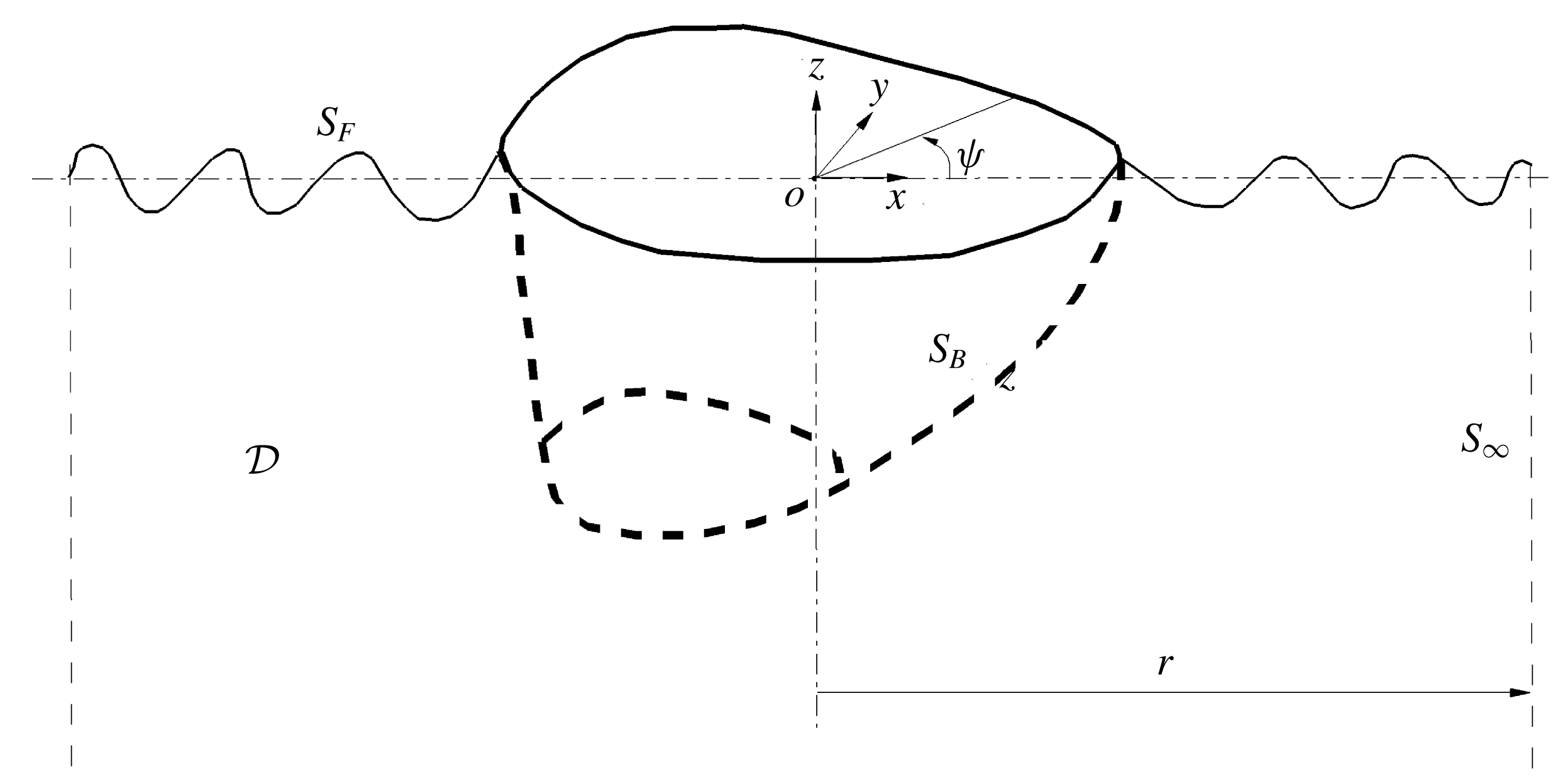For convenience, we define a supplemental cylindrical coordinate system ( $r,\unicode[STIX]{x1D713},z$ ) where $r$ represents the radius and $\unicode[STIX]{x1D713}$ denotes the azimuth. Figure 1 is a diagrammatic sketch of the wave–body interaction problem. Without loss of generality, we describe the general mathematical formation by referring to the wave radiation problem.

Figure 1.

Definition sketch of the wave–body interaction problem. A surface-piercing body floating on the free surface is forced to oscillate, radiating waves propagating away from the body. ${\mathcal{D}}(t)$ represents the instantaneous fluid domain, $S_{B}(t)$ the body surface, $S_{F}(t)$ the free surface, and $S_{\infty }(t)$ the fictitious vertical cylindrical closure boundary at far field. The Cartesian coordinate system $(x,y,z)$ and cylindrical coordinate system $(r,\unicode[STIX]{x1D713},z)$ share the same origin located on the mean free surface.

2.1 Nonlinear initial-boundary-value problem

The velocity potential $\unicode[STIX]{x1D719}(x,y,z,t)$ that describes the wave motion satisfies the Laplace equation anywhere in the fluid ${\mathcal{D}}(t)$ ,

(2.1) $$\begin{eqnarray}\displaystyle \unicode[STIX]{x1D6FB}^{2}\unicode[STIX]{x1D719}=0,\quad \text{in }{\mathcal{D}}(t). & & \displaystyle\end{eqnarray}$$

On the instantaneous free surface $S_{F}(t)$ , $\unicode[STIX]{x1D719}$ satisfies the kinematic and dynamic boundary conditions:

(2.2) $$\begin{eqnarray}\displaystyle \unicode[STIX]{x1D701}_{t}+\unicode[STIX]{x1D735}\unicode[STIX]{x1D719}\boldsymbol{\cdot }\unicode[STIX]{x1D735}\unicode[STIX]{x1D701}=\unicode[STIX]{x1D719}_{z},\quad \text{on }S_{F}(t), & & \displaystyle\end{eqnarray}$$

and

(2.3) $$\begin{eqnarray}\displaystyle \unicode[STIX]{x1D719}_{t}+\frac{1}{2}(\unicode[STIX]{x1D735}\unicode[STIX]{x1D719})^{2}+g\unicode[STIX]{x1D701}=\frac{T_{s}}{\unicode[STIX]{x1D70C}_{w}}\unicode[STIX]{x1D735}\boldsymbol{\cdot }\left(\frac{\unicode[STIX]{x1D735}\unicode[STIX]{x1D701}}{\sqrt{1+\unicode[STIX]{x1D735}\unicode[STIX]{x1D701}\boldsymbol{\cdot }\unicode[STIX]{x1D735}\unicode[STIX]{x1D701}}}\right),\quad \text{on }S_{F}(t), & & \displaystyle\end{eqnarray}$$

where $\unicode[STIX]{x1D735}\equiv (\unicode[STIX]{x2202}/\unicode[STIX]{x2202}x,\unicode[STIX]{x2202}/\unicode[STIX]{x2202}y,\unicode[STIX]{x2202}/\unicode[STIX]{x2202}z)$ , $t$ is time, $\unicode[STIX]{x1D701}(x,y,t)$ represents the free-surface elevation, $T_{s}$ denotes the surface tension, $\unicode[STIX]{x1D70C}_{w}$ is the fluid density, and $g$ is the gravitational acceleration. On the instantaneous body surface $S_{B}(t)$ , the normal velocity of the fluid ( $\unicode[STIX]{x1D719}_{n}$ ) is equal to the normal component of the velocity of the boundary

(2.4) $$\begin{eqnarray}\displaystyle \unicode[STIX]{x1D719}_{n}=\boldsymbol{V}\boldsymbol{\cdot }\boldsymbol{n},\quad \text{on }S_{B}(t), & & \displaystyle\end{eqnarray}$$

where $\boldsymbol{V}(x,y,z,t)$ represents the velocity of the body boundary and $\boldsymbol{n}$ is the unit normal vector of the body boundary pointing out of the fluid. In deep water, the fluid motion vanishes

(2.5) $$\begin{eqnarray}\displaystyle \unicode[STIX]{x1D735}\unicode[STIX]{x1D719}\rightarrow 0,\quad z\rightarrow -\infty . & & \displaystyle\end{eqnarray}$$

At the far field $S_{\infty }(t)$ , $\unicode[STIX]{x1D719}$ satisfies the radiation condition. The initial-boundary-value problem for $\unicode[STIX]{x1D719}$ is completely defined with the specification of the initial conditions of the free-surface elevation $(\unicode[STIX]{x1D701}(x,y,t=0))$ , the velocity potential on the free surface ( $\unicode[STIX]{x1D719}(x,y,z=\unicode[STIX]{x1D701},t=0)$ ) and the body boundary velocity $\boldsymbol{V}(x,y,z,t=0)$ .

One notes that in the absence of surface tension, the above formulation reduces to that for the gravity wave interaction with a body. The uniqueness of the solution for this well-known wave–body interaction problem has been proved by John (Reference John1950) in the limit of infinitesimal wave and body motions. When the surface tension effect is included, whether the solution of the above-stated three-dimensional problem is unique is not provided in the literature. To resolve this fundamental issue, we follow John (Reference John1950) to formulate the linearized problem and analyse the behaviour of the linear solution below.

2.2 Linearized frequency-domain problem

For harmonic body and wave motions, the velocity potential, free-surface elevation and body boundary velocity take the form

(2.6a-c ) $$\begin{eqnarray}\displaystyle \unicode[STIX]{x1D719}=\text{Re}\{\unicode[STIX]{x1D711}(x,y,z)\text{e}^{-\text{i}\unicode[STIX]{x1D714}_{0}t}\};\quad \unicode[STIX]{x1D701}=\text{Re}\{\unicode[STIX]{x1D702}(x,y)\text{e}^{-\text{i}\unicode[STIX]{x1D714}_{0}t}\};\quad \boldsymbol{V}=\text{Re}\{\boldsymbol{V}_{0}(x,y,z)\text{e}^{-\text{i}\unicode[STIX]{x1D714}_{0}t}\},\qquad \quad & & \displaystyle\end{eqnarray}$$

where $\unicode[STIX]{x1D714}_{0}$ is the frequency, $\unicode[STIX]{x1D711}$ , $\unicode[STIX]{x1D702}$ and $\boldsymbol{V}_{0}$ are the complex amplitudes of the velocity potential, free-surface elevation and body boundary velocity, respectively. For infinitesimal wave and body motions, the above nonlinear formulation can be linearized. The linearized boundary-value problem for $\unicode[STIX]{x1D711}$ is summarized as follows:

(2.7) $$\begin{eqnarray}\displaystyle & \displaystyle \unicode[STIX]{x1D6FB}^{2}\unicode[STIX]{x1D711}=0,\quad \text{on }\bar{{\mathcal{D}}}, & \displaystyle\end{eqnarray}$$

(2.8) $$\begin{eqnarray}\displaystyle & \displaystyle -K\unicode[STIX]{x1D711}+\unicode[STIX]{x1D711}_{z}+M\unicode[STIX]{x1D711}_{zzz}=0,\quad z=0, & \displaystyle\end{eqnarray}$$

(2.9) $$\begin{eqnarray}\displaystyle & \displaystyle \unicode[STIX]{x1D711}_{n}=\boldsymbol{V}_{0}\boldsymbol{\cdot }\boldsymbol{n},\quad \text{on }\bar{S}_{B}, & \displaystyle\end{eqnarray}$$

(2.10) $$\begin{eqnarray}\displaystyle & \displaystyle \unicode[STIX]{x1D735}\unicode[STIX]{x1D711}\rightarrow 0,\quad z\rightarrow -\infty , & \displaystyle\end{eqnarray}$$

(2.11) $$\begin{eqnarray}\displaystyle & \displaystyle \sqrt{r}(-\text{i}k_{0}\unicode[STIX]{x1D711}+\unicode[STIX]{x1D711}_{r})\rightarrow 0,\quad r\rightarrow \infty , & \displaystyle\end{eqnarray}$$

where

(2.12a,b ) $$\begin{eqnarray}\displaystyle K\equiv \frac{\unicode[STIX]{x1D714}_{0}^{2}}{g};\quad M\equiv \frac{T_{s}}{\unicode[STIX]{x1D70C}_{w}g} & & \displaystyle\end{eqnarray}$$

and the wavenumber of the propagating wave $k_{0}$ is related to $\unicode[STIX]{x1D714}_{0}$ by the dispersion relation

(2.13) $$\begin{eqnarray}\displaystyle K=k_{0}(1+\unicode[STIX]{x1D706}), & & \displaystyle\end{eqnarray}$$

where $\unicode[STIX]{x1D706}\equiv Mk_{0}^{2}$ . In the above, $\bar{S}_{B}$ is the mean body surface and $\bar{{\mathcal{D}}}$ is the mean fluid domain (bounded by $\bar{S}_{B}$ and the mean free surface $z=0$ ).

3 Proof of the existence of homogeneous solutions

Evans (Reference Evans1968) theoretically showed that the solution of the two-dimensional gravity–capillary wave generation problem by a surface-piercing body is not unique for any frequency. There exists a homogeneous solution that is completely dependent on the free-surface slope at the intersection of the body with the free surface. We here generalize his proof to the three-dimensional problem.

Figure 2.

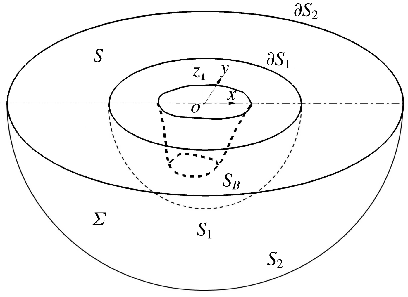
An illustrative sketch of the problem in the proof of the existence of a homogeneous solution. A fluid region $\unicode[STIX]{x1D6F4}$ is bounded by two hemispherical surfaces, $S_{1}$ and $S_{2}$ , and a portion of the mean free surface, $S$ . The surface-piercing body with mean body surface $\bar{S}_{B}$ is encircled by $S_{1}$ .

Consider the fluid region $\unicode[STIX]{x1D6F4}$ bounded by two hemispherical surfaces, $S_{1}$ and $S_{2}$ , and a portion of the mean free surface $S$ , as shown in figure 2. $S_{1}$ and $S_{2}$ intersect the mean free surface at the intersection lines $\unicode[STIX]{x2202}S_{1}(r_{f1},\unicode[STIX]{x1D713},0)$ and $\unicode[STIX]{x2202}S_{2}(r_{f2},\unicode[STIX]{x1D713},0)$ , respectively. The body is completely encircled by $S_{1}$ . The total energy in $\unicode[STIX]{x1D6F4}$ is given by

(3.1) $$\begin{eqnarray}\displaystyle E={\textstyle \frac{1}{2}}\unicode[STIX]{x1D70C}_{w}g\iint _{S}\unicode[STIX]{x1D701}^{2}\,\text{d}s+{\textstyle \frac{1}{2}}\unicode[STIX]{x1D70C}_{w}\iiint _{\unicode[STIX]{x1D6F4}}(\unicode[STIX]{x1D735}\unicode[STIX]{x1D719})^{2}\,\text{d}v+{\textstyle \frac{1}{2}}T_{s}\iint _{S}\unicode[STIX]{x1D735}\unicode[STIX]{x1D701}\boldsymbol{\cdot }\unicode[STIX]{x1D735}\unicode[STIX]{x1D701}\,\text{d}s, & & \displaystyle\end{eqnarray}$$

where the first, second and third terms on the right-hand side of (3.1) represent the potential energy, kinetic energy and surface capillary energy, respectively (Wehausen & Laitone Reference Wehausen and Laitone1960). After taking the time derivative of equation (3.1) and applying Green’s theorem for the volume integral, we obtain the rate of change of energy as

(3.2) $$\begin{eqnarray}\displaystyle \frac{\text{d}E}{\text{d}t}=\unicode[STIX]{x1D70C}_{w}\iint _{S+S_{1}+S_{2}}\unicode[STIX]{x1D719}_{t}\unicode[STIX]{x1D719}_{n}\,\text{d}s+\unicode[STIX]{x1D70C}_{w}g\iint _{S}\unicode[STIX]{x1D701}\unicode[STIX]{x1D701}_{t}\,\text{d}s+T_{s}\iint _{S}\unicode[STIX]{x1D735}\unicode[STIX]{x1D701}\boldsymbol{\cdot }\unicode[STIX]{x1D735}\unicode[STIX]{x1D701}_{t}\,\text{d}s, & & \displaystyle\end{eqnarray}$$

where $\unicode[STIX]{x1D719}_{n}$ denotes the fluid velocity in the normal direction to the boundary pointing out of the fluid. Using relation

(3.3) $$\begin{eqnarray}\displaystyle \iint _{S}\unicode[STIX]{x1D735}\unicode[STIX]{x1D701}\boldsymbol{\cdot }\unicode[STIX]{x1D735}\unicode[STIX]{x1D701}_{t}\,\text{d}s=\iint _{S}[\unicode[STIX]{x1D735}\boldsymbol{\cdot }(\unicode[STIX]{x1D701}_{t}\unicode[STIX]{x1D735}\unicode[STIX]{x1D701})-\unicode[STIX]{x1D701}_{t}\unicode[STIX]{x1D6FB}^{2}\unicode[STIX]{x1D701}]\,\text{d}s & & \displaystyle\end{eqnarray}$$

and imposing the linearized dynamic boundary condition on $S$ , we have

(3.4) $$\begin{eqnarray}\displaystyle \frac{\text{d}E}{\text{d}t}=\unicode[STIX]{x1D70C}_{w}\iint _{S_{2}}\unicode[STIX]{x1D719}_{t}\unicode[STIX]{x1D719}_{n}\,\text{d}s-\unicode[STIX]{x1D70C}_{w}\iint _{S_{1}}\unicode[STIX]{x1D719}_{t}\unicode[STIX]{x1D719}_{n}\,\text{d}s+T_{s}\oint _{\unicode[STIX]{x2202}S_{2}}\unicode[STIX]{x1D701}_{t}\unicode[STIX]{x1D735}\unicode[STIX]{x1D701}\boldsymbol{\cdot }\unicode[STIX]{x1D749}\,\text{d}l-T_{s}\oint _{\unicode[STIX]{x2202}S_{1}}\unicode[STIX]{x1D701}_{t}\unicode[STIX]{x1D735}\unicode[STIX]{x1D701}\boldsymbol{\cdot }\unicode[STIX]{x1D749}\,\text{d}l,\quad & & \displaystyle\end{eqnarray}$$

where $\unicode[STIX]{x2202}S_{i}$ , $i=1$ and 2, represents the intersection line of hemispherical surface $S_{i}$ with the mean free surface ( $z=0$ ), and $\unicode[STIX]{x1D749}$ is the unit normal vector of the intersection line on the mean free surface pointing out of the body.

For the harmonic motion at frequency $\unicode[STIX]{x1D714}_{0}$ , the average rate of change of $E$ is given by

(3.5) $$\begin{eqnarray}\displaystyle \overline{\frac{\text{d}E}{\text{d}t}}={\mathcal{F}}_{1}-{\mathcal{F}}_{2}, & & \displaystyle\end{eqnarray}$$

where ${\mathcal{F}}_{i}$ , $i=1,2$ , represents the average energy flux through $S_{i}$ and is given by

(3.6) $$\begin{eqnarray}\displaystyle {\mathcal{F}}_{i} & = & \displaystyle -\frac{\unicode[STIX]{x1D714}_{0}}{2\unicode[STIX]{x03C0}}\int _{0}^{2\unicode[STIX]{x03C0}/\unicode[STIX]{x1D714}_{0}}\,\text{d}t\left\{\unicode[STIX]{x1D70C}_{w}\iint _{S_{i}}\unicode[STIX]{x1D719}_{t}\unicode[STIX]{x1D719}_{n}\,\text{d}s+T_{s}\oint _{\unicode[STIX]{x2202}S_{i}}\unicode[STIX]{x1D701}_{t}\unicode[STIX]{x1D735}\unicode[STIX]{x1D701}\boldsymbol{\cdot }\unicode[STIX]{x1D749}\,\text{d}l\right\}\nonumber\\ \displaystyle & = & \displaystyle \frac{\unicode[STIX]{x1D70C}_{w}\unicode[STIX]{x1D714}_{0}}{2}\text{Im}\left\{\iint _{S_{i}}\unicode[STIX]{x1D711}^{\ast }\unicode[STIX]{x1D711}_{n}\,\text{d}s+\frac{T_{s}}{\unicode[STIX]{x1D70C}_{w}}\oint _{\unicode[STIX]{x2202}S_{i}}\unicode[STIX]{x1D702}^{\ast }\unicode[STIX]{x1D702}_{\unicode[STIX]{x1D70F}}\,\text{d}l\right\}\end{eqnarray}$$

with $\ast$ denoting the complex conjugate.

We now let $S_{1}$ contract to become $\bar{S}_{B}$ and $S_{2}$ expand to become $\bar{S}_{\infty }$ . On $\bar{S}_{\infty }$ , $\unicode[STIX]{x1D711}$ satisfies the radiation condition (2.11) and takes the general form

(3.7) $$\begin{eqnarray}\displaystyle \unicode[STIX]{x1D711}(r,\unicode[STIX]{x1D713},z)=\mathop{\sum }_{m=0}^{\infty }\frac{C_{m}}{\sqrt{k_{0}r}}\text{e}^{k_{0}z+\text{i}k_{0}r}\cos (m\unicode[STIX]{x1D713}),\quad r\rightarrow \infty , & & \displaystyle\end{eqnarray}$$

where $C_{m}$ represents the complex amplitude of the outgoing wave with the azimuthal wavenumber $m$ . Using (3.7), we obtain the associated free-surface elevation $\unicode[STIX]{x1D702}$ (from the linearized dynamic free-surface boundary condition). By the use of a cylindrical vertical surface for $\bar{S}_{\infty }$ , we get

(3.8) $$\begin{eqnarray}\displaystyle {\mathcal{F}}_{2}=\unicode[STIX]{x03C0}\frac{\unicode[STIX]{x1D70C}_{w}\unicode[STIX]{x1D714}_{0}}{4K}(1+3\unicode[STIX]{x1D706})\mathop{\sum }_{m=0}^{\infty }|C_{m}|^{2}. & & \displaystyle\end{eqnarray}$$

For the homogeneous problem, $\unicode[STIX]{x1D719}_{n}=0$ on $\bar{S}_{B}$ . From (3.6), we obtain

(3.9) $$\begin{eqnarray}\displaystyle {\mathcal{F}}_{1}=\frac{T_{s}\unicode[STIX]{x1D714}_{0}}{2}\text{Im}\left\{\oint _{\unicode[STIX]{x2202}\bar{S}_{B}}\unicode[STIX]{x1D702}^{\ast }\unicode[STIX]{x1D702}_{\unicode[STIX]{x1D749}}\,\text{d}l\right\}. & & \displaystyle\end{eqnarray}$$

From the conservation of energy, we have ${\mathcal{F}}_{1}-{\mathcal{F}}_{2}=0$ from which we obtain

(3.10) $$\begin{eqnarray}\displaystyle \mathop{\sum }_{m=0}^{\infty }|C_{m}|^{2}=\frac{2T_{s}K}{\unicode[STIX]{x03C0}\unicode[STIX]{x1D70C}_{w}(1+3\unicode[STIX]{x1D706})}\text{Im}\left\{\oint _{\unicode[STIX]{x2202}\bar{S}_{B}}\unicode[STIX]{x1D702}^{\ast }\unicode[STIX]{x1D702}_{\unicode[STIX]{x1D749}}\,\text{d}l\right\}. & & \displaystyle\end{eqnarray}$$

If $\unicode[STIX]{x1D702}_{\unicode[STIX]{x1D749}}\neq 0$ on the waterline of the body, $\sum _{m}|C_{m}|^{2}\neq 0$ so that $\unicode[STIX]{x1D711}\neq 0$ at the far field, showing the existence of a non-trivial homogeneous solution. If $\unicode[STIX]{x1D702}_{\unicode[STIX]{x1D749}}=0$ on the waterline of the body, $C_{m}=0$ for all $m$ and $\unicode[STIX]{x1D711}=0$ at the far field so that the homogeneous solution is trivial. In the absence of surface tension ( $T_{s}=0$ ), we also have $\sum _{m}|C_{m}|^{2}=0$ and $\unicode[STIX]{x1D711}=0$ , consistent with the proof of John (Reference John1950) for the gravity wave problem.

In summary, the above analysis shows that for the problem of gravity–capillary wave interaction with an arbitrary three-dimensional body, the linearized boundary-value problem possesses a non-trivial homogeneous solution at any frequency if the free surface has a non-zero slope at the waterline of the body in the direction normal to the waterline. In this case, the solution of the general boundary-value problem is non-unique. On the other hand, the boundary-value problem possesses a trivial homogeneous solution and the solution of the boundary-value problem is unique only under the condition that the free surface has a zero slope at the waterline in the horizontal direction normal to the waterline.

We remark that the homogeneous solution is defined to be the boundary-value solution when the body (or wave maker) is still. The non-trivial homogeneous solution, which is given in terms of the (harmonic) amplitude of free-surface slope at the waterline of the body, represents an outgoing propagating wave. For a non-zero surface slope at the waterline, the surface tension has a component in the vertical direction, which would do work with the vertical displacement of the free surface at the waterline (see (3.9)). Energy input to the system against the work done by the surface tension at the waterline is needed to maintain the steady-state outgoing wave system. Mathematically this is achieved by specifying the harmonic amplitude of free-surface slope oscillation. If the amplitude of slope oscillation is zero (corresponding to no energy input to the system), this wave does not radiate any energy to the far field. This corresponds to the trivial homogeneous solution case. The objective of this paper is to show that the non-trivial homogeneous solution can grow in space/time by taking energy from the base ring waves (generated by forced body motion) through subharmonic resonant wave–wave interactions.

We also note that our proof of the existence of non-trivial homogeneous gravity–capillary wave solutions for the three-dimensional case is consistent with the two-dimensional case of Evans (Reference Evans1968). Physically, the wave generation by a three-dimensional body is identical to that in the two-dimensional case. Mathematically, however, the two-dimensional solution cannot be directly deduced from the three-dimensional solution in a simple way. This is because the wave elevation of the radiated wave in the two-dimensional case remains constant as it propagates away from the body, while the total radiated wave elevation in the three-dimensional case decays with the distance ( $r$ ) from the body as $r^{-1/2}$ . This is reflected by different forms of the radiation conditions in three dimensions (2.11) and two dimensions (equation (3.3) in Evans Reference Evans1968). As a result, a Hankel function (in $r$ ) is used in three-dimensional problems (see §§ 4.1 and 4.2) while a Fourier series (in $x$ ) is used in two-dimensional problems.

4 Subharmonic interaction of a radial cross-wave with an axial-symmetric wave by a vertical circular cylinder

In order to study the subharmonic resonant interaction of a progressive axial-symmetric wave and a radial cross-wave, we employ Whitham’s average Lagrangian method (Whitham Reference Whitham1974). For analytic illustration, we here consider the wave-making problem of a vertical circular cylinder that undergoes a specified radial swelling–contraction deformation in the horizontal plane. Deep water is assumed. The cylinder has a radius of $r_{1}$ . The vertical boundary of the cylinder has a displacement in the radial direction $\unicode[STIX]{x1D712}(z,t)$ . For this body geometry, we can derive closed-form solutions for forced axial-symmetric waves and radial cross-waves. For the problem with general body geometries, numerical procedures need to be used for obtaining the solutions of interacting waves.

We first derive the Lagrangian from first principles for the interaction problem of gravity–capillary waves with a vertical circular cylinder (Luke Reference Luke1967; Miles Reference Miles1976, Reference Miles1984; Miles & Becker Reference Miles and Becker1988; Becker & Miles Reference Becker and Miles1992),

(4.1) $$\begin{eqnarray}\displaystyle 2L & = & \displaystyle \iiint _{{\mathcal{D}}}\unicode[STIX]{x1D719}\unicode[STIX]{x1D6FB}^{2}\unicode[STIX]{x1D719}r\,\text{d}r\,\text{d}\unicode[STIX]{x1D713}\,\text{d}z\nonumber\\ \displaystyle & & \displaystyle +\,\iint _{S_{F}}\left[\unicode[STIX]{x1D719}(2\unicode[STIX]{x1D701}_{t}-\unicode[STIX]{x1D719}_{z}+\unicode[STIX]{x1D735}\unicode[STIX]{x1D719}\boldsymbol{\cdot }\unicode[STIX]{x1D735}\unicode[STIX]{x1D701})-g\unicode[STIX]{x1D701}^{2}-2\frac{T_{s}}{\unicode[STIX]{x1D70C}_{w}}\left(\sqrt{1+\unicode[STIX]{x1D735}\unicode[STIX]{x1D701}\boldsymbol{\cdot }\unicode[STIX]{x1D735}\unicode[STIX]{x1D701}}-1\right)\right]_{z=\unicode[STIX]{x1D701}}r\,\text{d}r\,\text{d}\unicode[STIX]{x1D713}\nonumber\\ \displaystyle & & \displaystyle +\,\iint _{S_{B}}[\unicode[STIX]{x1D719}(\unicode[STIX]{x1D719}_{r}-\unicode[STIX]{x1D735}\unicode[STIX]{x1D712}\boldsymbol{\cdot }\unicode[STIX]{x1D735}\unicode[STIX]{x1D719}-2\unicode[STIX]{x1D712}_{t})-gz^{2}\unicode[STIX]{x1D712}_{z}]_{r=r_{1}+\unicode[STIX]{x1D712}}r\,\text{d}\unicode[STIX]{x1D713}\,\text{d}z-\iint _{S_{\infty }}\unicode[STIX]{x1D719}\unicode[STIX]{x1D719}_{r}r_{2}\,\text{d}\unicode[STIX]{x1D713}\,\text{d}z,\end{eqnarray}$$

where $r_{2}$ is the radius of cylindrical surface $S_{\infty }$ at the far field. In the general three-dimensional case, the radiated wave amplitude in the far field decays with the distance ( $r$ ) from the body as $r^{-1/2}$ as $r\rightarrow \infty$ . The corresponding velocity potential ( $\unicode[STIX]{x1D719}$ ) and radial velocity ( $\unicode[STIX]{x1D719}_{r}$ ) also decay like $r^{-1/2}$ as $r\rightarrow \infty$ . As a result, the last integral in (4.1) would approach to a non-zero quantity. In the work of Becker & Miles (Reference Becker and Miles1992), however, the value of this integral vanishes since both $\unicode[STIX]{x1D719}$ and $\unicode[STIX]{x1D719}_{r}$ are assumed to decay exponentially with $r$ as $r\rightarrow \infty$ .

We consider the perturbation expansion of the velocity potential and surface elevation in the dimensionless form

(4.2) $$\begin{eqnarray}\displaystyle (k_{0}^{2}/\unicode[STIX]{x1D714}_{0})\unicode[STIX]{x1D719}=\unicode[STIX]{x1D707}\unicode[STIX]{x1D719}_{1}+\unicode[STIX]{x1D700}\unicode[STIX]{x1D719}_{0}+O(\unicode[STIX]{x1D707}\unicode[STIX]{x1D700},\unicode[STIX]{x1D707}^{2},\unicode[STIX]{x1D700}^{2}) & & \displaystyle\end{eqnarray}$$

and

(4.3) $$\begin{eqnarray}\displaystyle k_{0}\unicode[STIX]{x1D701}=\unicode[STIX]{x1D707}\unicode[STIX]{x1D701}_{1}+\unicode[STIX]{x1D700}\unicode[STIX]{x1D701}_{0}+O(\unicode[STIX]{x1D707}\unicode[STIX]{x1D700},\unicode[STIX]{x1D707}^{2},\unicode[STIX]{x1D700}^{2}), & & \displaystyle\end{eqnarray}$$

where $(\unicode[STIX]{x1D719}_{0},\unicode[STIX]{x1D701}_{0})$ represent the (normalized) linear progressive axial-symmetric (ring) wave forced by the swelling–contraction motion of the cylinder boundary, $(\unicode[STIX]{x1D719}_{1},\unicode[STIX]{x1D701}_{1})$ represent the (normalized) linear progressive radial cross-wave mode, and $\unicode[STIX]{x1D700}\equiv k_{0}a$ (or $\unicode[STIX]{x1D707}$ ) is a measure of the order of magnitude of the forced axial-symmetric wave (or cross-wave), where $a$ is the characteristic amplitude of the body’s boundary displacement. In this study, our focus is on the initial growth of cross-waves through energy transfer from the forced axial-symmetric wave, but not on the long-time evolution of their interactions. It is thus sufficient to assume $\unicode[STIX]{x1D707}\ll \unicode[STIX]{x1D700}$ . For convenience, the frequency of the axial-symmetric wave is chosen to be $2\unicode[STIX]{x1D714}_{0}$ while that of the cross-wave is $\unicode[STIX]{x1D714}_{0}$ to reflect their subharmonic relation. Being consistent with the normalization of $\unicode[STIX]{x1D719}$ and $\unicode[STIX]{x1D701}$ in (4.2) and (4.3), we use the dimensionless spatial and temporal independent variables in the following analysis

(4.4a-c ) $$\begin{eqnarray}\displaystyle \unicode[STIX]{x1D70C}\equiv k_{0}r,\quad \unicode[STIX]{x1D709}\equiv k_{0}z,\quad \unicode[STIX]{x1D703}\equiv \unicode[STIX]{x1D714}_{0}t. & & \displaystyle\end{eqnarray}$$

We express the cross-wave with envelope in the form

(4.5a,b ) $$\begin{eqnarray}\displaystyle \unicode[STIX]{x1D719}_{1}=\text{Re}\{A(R,\unicode[STIX]{x1D70F})\unicode[STIX]{x1D711}_{1}(\unicode[STIX]{x1D70C},\unicode[STIX]{x1D709},\unicode[STIX]{x1D713})\text{e}^{-\text{i}\unicode[STIX]{x1D703}}\},\quad \unicode[STIX]{x1D701}_{1}=\text{Re}\{A(R,\unicode[STIX]{x1D70F})\unicode[STIX]{x1D702}_{1}(\unicode[STIX]{x1D70C},\unicode[STIX]{x1D713})\text{e}^{-\text{i}\unicode[STIX]{x1D703}}\}, & & \displaystyle\end{eqnarray}$$

where $A$ is the complex amplitude that depends on the slowly varying spatial and temporal variables defined as

(4.6a,b ) $$\begin{eqnarray}\displaystyle R=2\unicode[STIX]{x1D700}\unicode[STIX]{x1D70C},\quad \unicode[STIX]{x1D70F}=\unicode[STIX]{x1D700}\unicode[STIX]{x1D703}. & & \displaystyle\end{eqnarray}$$

By using the average Lagrangian method with (4.1), we shall find an evolution equation that governs the growth (or decay) of $A$ in the subharmonic resonant interaction of the cross-wave with the forced axial-symmetric wave. Before doing that, we shall derive the solutions of the cross-wave mode ( $\unicode[STIX]{x1D711}_{1}$ , $\unicode[STIX]{x1D702}_{1}$ ) and the forced axial-symmetric wave ( $\unicode[STIX]{x1D719}_{0}$ , $\unicode[STIX]{x1D701}_{0}$ ).

4.1 Linear homogeneous cross-wave solution

The cross-wave $(\unicode[STIX]{x1D711}_{1},\unicode[STIX]{x1D702}_{1})$ is given by the homogeneous solution of the boundary-value problem with a specified (unit-amplitude) radial slope of the free surface at the waterline of the vertical circular cylinder:

(4.7a-c ) $$\begin{eqnarray}\displaystyle \unicode[STIX]{x1D702}_{1\unicode[STIX]{x1D70C}}=\cos m\unicode[STIX]{x1D713},\quad \unicode[STIX]{x1D70C}=\unicode[STIX]{x1D70C}_{1},\quad \unicode[STIX]{x1D709}=0, & & \displaystyle\end{eqnarray}$$

where $m=0,1,\ldots$ is the azimuthal wavenumber. The homogeneous boundary-value problem is composed of

(4.8) $$\begin{eqnarray}\displaystyle & \displaystyle \unicode[STIX]{x1D6FB}^{2}\unicode[STIX]{x1D711}_{1}=0,\quad \unicode[STIX]{x1D70C}_{1}\leqslant \unicode[STIX]{x1D70C}<\infty ,\quad 0\leqslant \unicode[STIX]{x1D713}<2\unicode[STIX]{x03C0},\quad -\infty <\unicode[STIX]{x1D709}\leqslant 0, & \displaystyle\end{eqnarray}$$

(4.9) $$\begin{eqnarray}\displaystyle & \displaystyle -(1+\unicode[STIX]{x1D706})\unicode[STIX]{x1D711}_{1}+\unicode[STIX]{x1D711}_{1\unicode[STIX]{x1D709}}+\unicode[STIX]{x1D706}\unicode[STIX]{x1D711}_{1\unicode[STIX]{x1D709}\unicode[STIX]{x1D709}\unicode[STIX]{x1D709}}=0,\quad \unicode[STIX]{x1D709}=0, & \displaystyle\end{eqnarray}$$

(4.10) $$\begin{eqnarray}\displaystyle & \displaystyle \unicode[STIX]{x1D711}_{1\unicode[STIX]{x1D70C}}=0,\quad \unicode[STIX]{x1D70C}=\unicode[STIX]{x1D70C}_{1}, & \displaystyle\end{eqnarray}$$

and the deep water condition $\unicode[STIX]{x1D735}\unicode[STIX]{x1D711}\rightarrow 0$ as $\unicode[STIX]{x1D709}\rightarrow -\infty$ as well as the radiation condition at the far field, which physically states that the cross-wave propagates away from the body as $\unicode[STIX]{x1D70C}\rightarrow \infty$ .

The analytical homogeneous solution for a vertical circular cylinder is derived in appendix A, which can be expressed as

(4.11a,b ) $$\begin{eqnarray}\displaystyle \unicode[STIX]{x1D711}_{1}=\bar{\unicode[STIX]{x1D711}}_{m}(\unicode[STIX]{x1D70C},\unicode[STIX]{x1D709})\cos m\unicode[STIX]{x1D713}\quad \text{and}\quad \unicode[STIX]{x1D702}_{1}=\bar{\unicode[STIX]{x1D702}}_{m}(\unicode[STIX]{x1D70C})\cos m\unicode[STIX]{x1D713}, & & \displaystyle\end{eqnarray}$$

where

(4.12) $$\begin{eqnarray}\displaystyle \bar{\unicode[STIX]{x1D711}}_{m}=-\text{i}\frac{\unicode[STIX]{x1D706}}{\unicode[STIX]{x03C0}}\int _{0}^{\infty }\frac{2K_{m}(k\unicode[STIX]{x1D70C})}{K_{m}^{\prime }(k\unicode[STIX]{x1D70C}_{1})}\frac{[k(1-\unicode[STIX]{x1D706}k^{2})\cos k\unicode[STIX]{x1D709}+K\sin k\unicode[STIX]{x1D709}]}{k^{2}(1-\unicode[STIX]{x1D706}k^{2})^{2}+K^{2}}\,\text{d}k-\text{i}\frac{2\unicode[STIX]{x1D706}}{1+3\unicode[STIX]{x1D706}}\frac{H_{m}^{(1)}(\unicode[STIX]{x1D70C})}{H_{m}^{(1)^{\prime }}(\unicode[STIX]{x1D70C}_{1})}\text{e}^{\unicode[STIX]{x1D709}}\qquad & & \displaystyle\end{eqnarray}$$

and

(4.13) $$\begin{eqnarray}\displaystyle \bar{\unicode[STIX]{x1D702}}_{m}=\frac{\unicode[STIX]{x1D706}}{\unicode[STIX]{x03C0}}\int _{0}^{\infty }\frac{2K_{m}(k\unicode[STIX]{x1D70C})}{K_{m}^{\prime }(k\unicode[STIX]{x1D70C}_{1})}\frac{Kk}{k^{2}(1-\unicode[STIX]{x1D706}k^{2})^{2}+K^{2}}\,\text{d}k+\frac{2\unicode[STIX]{x1D706}}{1+3\unicode[STIX]{x1D706}}\frac{H_{m}^{(1)}(\unicode[STIX]{x1D70C})}{H_{m}^{(1)^{\prime }}(\unicode[STIX]{x1D70C}_{1})}, & & \displaystyle\end{eqnarray}$$

where $\text{K}_{m}$ is the $m$ th-order modified Bessel function of the second kind and the prime symbol denotes the derivative of the function with respect to its argument. The cross-wave solution ( $\unicode[STIX]{x1D711}_{m}$ , $\unicode[STIX]{x1D702}_{m}$ ) consists of the evanescent component (corresponding to the integral term), which vanishes exponentially with the distance from the body, and the propagating component which persists into the far field. It is worth noting that the gravity–capillary cross-wave solution obtained here represents an outgoing propagating wave but not a standing wave as used in the previous studies (e.g. Garrett Reference Garrett1970; Mahoney Reference Mahoney1972; Becker & Miles Reference Becker and Miles1992). There are two sources of energy dissipation in cross-wave motion. One is the work done by the vertical component of surface tension force at the waterline of the body (since the radial slope of the free surface is non-zero for cross-waves), and the other is radiation of energy associated with the outgoing propagation of cross-waves.

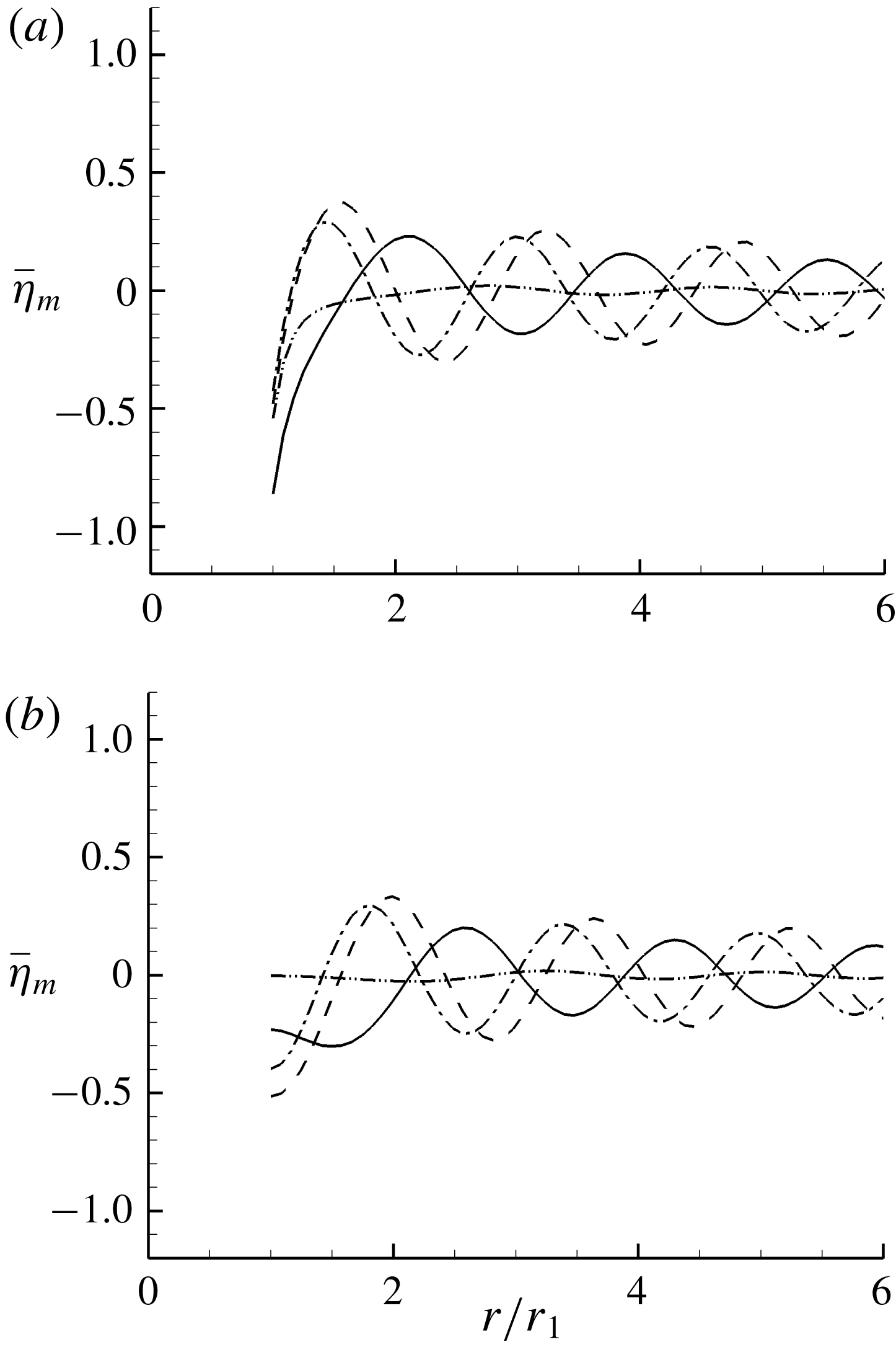
Figures 3(a) and 3(b) display sample free-surface profiles of axial-symmetric ( $m=0$ ) and asymmetric ( $m\neq 0$ ) cross-wave modes. For $m\ll k_{0}r_{1}$ , the cross-wave profile is dominated by the propagating wave component while for $m\gg k_{0}r_{1}$ , it is dominated by the evanescent component trapped around the body, as shown in figures 3(a) and 3(b). In the former, energy dissipation in cross-wave motion is mainly through wave radiation to the far field while in the latter, it is mainly due to the work done by surface tension at the waterline.

Figure 3.

(a) Real and (b) imaginary parts of cross-wave profiles, $\bar{\unicode[STIX]{x1D702}}_{m}$ , for a vertical circular cylinder with $k_{0}r_{1}=3.98$ . The plotted curves are for azimuthal wavenumber $m=0$ (— ⋅ —), $m=3$ (– – –), $m=5$ (——), and $m=7$ (— ⋅ ⋅ —).

4.2 Linear forced axial-symmetric wave solution

To find the solution of a forced axial-symmetric wave, we consider the swelling–contraction motion of the vertical boundary of the vertical circular cylinder with the (dimensionless) radial displacement given by

(4.14) $$\begin{eqnarray}\displaystyle \unicode[STIX]{x1D6EF}=\unicode[STIX]{x1D700}f(\unicode[STIX]{x1D709})\sin 2\unicode[STIX]{x1D703}, & & \displaystyle\end{eqnarray}$$

where $\unicode[STIX]{x1D6EF}=k_{0}\unicode[STIX]{x1D712}$ , $\unicode[STIX]{x1D700}\equiv k_{0}a$ is the (normalized) oscillation amplitude and $f(\unicode[STIX]{x1D709})$ is the wave-maker function on the vertical surface of the cylinder. We express $\unicode[STIX]{x1D719}_{0}$ and $\unicode[STIX]{x1D701}_{0}$ in the form

(4.15a,b ) $$\begin{eqnarray}\displaystyle \unicode[STIX]{x1D719}_{0}=\text{Re}\{\unicode[STIX]{x1D711}_{0}\text{e}^{-\text{i}2\unicode[STIX]{x1D703}}\};\quad \unicode[STIX]{x1D701}_{0}=\text{Re}\{\unicode[STIX]{x1D702}_{0}\text{e}^{-\text{i}2\unicode[STIX]{x1D703}}\}. & & \displaystyle\end{eqnarray}$$

The linearized boundary-value problem for the forced axial-symmetric wave $\unicode[STIX]{x1D719}_{0}$ and $\unicode[STIX]{x1D701}_{0}$ consists of

(4.16) $$\begin{eqnarray}\displaystyle & \displaystyle \unicode[STIX]{x1D6FB}^{2}\unicode[STIX]{x1D711}_{0}=0,\quad \unicode[STIX]{x1D70C}_{1}\leqslant \unicode[STIX]{x1D70C}<\infty ,\quad 0\leqslant \unicode[STIX]{x1D713}<2\unicode[STIX]{x03C0},\quad -\infty <\unicode[STIX]{x1D709}\leqslant 0, & \displaystyle\end{eqnarray}$$

(4.17) $$\begin{eqnarray}\displaystyle & \displaystyle -4(1+\unicode[STIX]{x1D706})\unicode[STIX]{x1D711}_{0}+\unicode[STIX]{x1D711}_{0\unicode[STIX]{x1D709}}+\unicode[STIX]{x1D706}\unicode[STIX]{x1D711}_{0\unicode[STIX]{x1D709}\unicode[STIX]{x1D709}\unicode[STIX]{x1D709}}=0,\quad \unicode[STIX]{x1D709}=0, & \displaystyle\end{eqnarray}$$

(4.18) $$\begin{eqnarray}\displaystyle & \displaystyle \unicode[STIX]{x1D711}_{0\unicode[STIX]{x1D70C}}=2f(\unicode[STIX]{x1D709}),\quad \unicode[STIX]{x1D70C}=\unicode[STIX]{x1D70C}_{1}, & \displaystyle\end{eqnarray}$$

plus the deep water condition $\unicode[STIX]{x1D735}\unicode[STIX]{x1D711}_{0}\rightarrow 0$ as $\unicode[STIX]{x1D709}\rightarrow -\infty$ and the radiation condition as $\unicode[STIX]{x1D70C}\rightarrow \infty$ . To ensure a unique solution of $\unicode[STIX]{x1D719}_{0}$ and $\unicode[STIX]{x1D702}_{0}$ , the condition $\unicode[STIX]{x1D702}_{0\unicode[STIX]{x1D70C}}=0$ at the waterline of the body is imposed.

The solution of the above boundary-value problem for $\unicode[STIX]{x1D711}_{0}$ is obtained to be (Rhodes-Robinson Reference Rhodes-Robinson1971; Becker & Miles Reference Becker and Miles1992)

(4.19) $$\begin{eqnarray}\displaystyle \unicode[STIX]{x1D711}_{0}(\unicode[STIX]{x1D70C},\unicode[STIX]{x1D709}) & = & \displaystyle \left\{\frac{4}{\unicode[STIX]{x03C0}}\int _{0}^{\infty }\frac{K_{0}(k\unicode[STIX]{x1D70C})}{K_{0}^{\prime }(k\unicode[STIX]{x1D70C}_{1})}\frac{[k(1-\unicode[STIX]{x1D706}k^{2})\sin k\unicode[STIX]{x1D709}+4(1+\unicode[STIX]{x1D706})\cos k\unicode[STIX]{x1D709}]}{k^{2}(1-\unicode[STIX]{x1D706}k^{2})^{2}+[4(1+\unicode[STIX]{x1D706})]^{2}}\frac{G(k)}{k}\,\text{d}k\right\}\nonumber\\ \displaystyle & & \displaystyle +\,4\frac{1+\unicode[STIX]{x1D706}\unicode[STIX]{x1D707}_{0}^{2}}{1+3\unicode[STIX]{x1D706}\unicode[STIX]{x1D707}_{0}^{2}}\text{e}^{\unicode[STIX]{x1D707}_{0}\unicode[STIX]{x1D709}}\frac{H_{0}^{(1)}(\unicode[STIX]{x1D707}_{0}\unicode[STIX]{x1D70C})}{H_{0}^{(1)^{\prime }}(\unicode[STIX]{x1D707}_{0}\unicode[STIX]{x1D70C}_{1})}\int _{-\infty }^{0}f(\unicode[STIX]{x1D717})\text{e}^{\unicode[STIX]{x1D707}_{0}\unicode[STIX]{x1D717}}\,\text{d}\unicode[STIX]{x1D717}\end{eqnarray}$$

and

(4.20) $$\begin{eqnarray}\displaystyle \unicode[STIX]{x1D702}_{0}(\unicode[STIX]{x1D70C}) & = & \displaystyle \left\{\frac{2\text{i}}{\unicode[STIX]{x03C0}}\int _{0}^{\infty }\frac{K_{0}(k\unicode[STIX]{x1D70C})}{K_{0}^{\prime }(k\unicode[STIX]{x1D70C}_{1})}\frac{k(1-\unicode[STIX]{x1D706}k^{2})G(k)}{k^{2}(1-\unicode[STIX]{x1D706}k^{2})^{2}+[4(1+\unicode[STIX]{x1D706})]^{2}}\,\text{d}k\right\}\nonumber\\ \displaystyle & & \displaystyle +\,2\text{i}\unicode[STIX]{x1D707}_{0}\frac{1+\unicode[STIX]{x1D706}\unicode[STIX]{x1D707}_{0}^{2}}{1+3\unicode[STIX]{x1D706}\unicode[STIX]{x1D707}_{0}^{2}}\frac{H_{0}^{(1)}(\unicode[STIX]{x1D707}_{0}\unicode[STIX]{x1D70C})}{H_{0}^{(1)^{\prime }}(\unicode[STIX]{x1D707}_{0}\unicode[STIX]{x1D70C}_{1})}\int _{-\infty }^{0}f(\unicode[STIX]{x1D717})\text{e}^{\unicode[STIX]{x1D707}_{0}\unicode[STIX]{x1D717}}\,\text{d}\unicode[STIX]{x1D717},\end{eqnarray}$$

where

(4.21) $$\begin{eqnarray}\displaystyle G(k)\equiv \int _{-\infty }^{0}[k(1-\unicode[STIX]{x1D706}k^{2})\sin k\unicode[STIX]{x1D717}+4(1+\unicode[STIX]{x1D706})\cos k\unicode[STIX]{x1D717}]f(\unicode[STIX]{x1D717})\,\text{d}\unicode[STIX]{x1D717} & & \displaystyle\end{eqnarray}$$

and $\unicode[STIX]{x1D707}_{0}$ is the wavenumber of the forced outgoing wave corresponding to the frequency $2\unicode[STIX]{x1D714}_{0}$ , which is given by the real root of the dispersion relation

(4.22) $$\begin{eqnarray}\displaystyle \unicode[STIX]{x1D707}_{0}(1+\unicode[STIX]{x1D706}\unicode[STIX]{x1D707}_{0}^{2})=4(1+\unicode[STIX]{x1D706}). & & \displaystyle\end{eqnarray}$$

By letting $\unicode[STIX]{x1D706}=0$ , corresponding to zero surface tension, (4.20) reduces to Havelock’s gravity wave solution (Havelock Reference Havelock1929).

From (4.20), it is seen that the forced axial-symmetric wave solution generally consists of an evanescent component (inside the curly brackets) and a propagating component. Depending on the wave-maker function $f(\unicode[STIX]{x1D709})$ , the generated wave could contain either an evanescent or propagating component only. For example, only the evanescent wave component can be generated if we set

(4.23) $$\begin{eqnarray}\displaystyle f(\unicode[STIX]{x1D709})=\frac{\unicode[STIX]{x1D707}_{p}}{\unicode[STIX]{x1D707}_{0}}\cos (\unicode[STIX]{x1D707}_{p}\unicode[STIX]{x1D709})+\sin (\unicode[STIX]{x1D707}_{p}\unicode[STIX]{x1D709}), & & \displaystyle\end{eqnarray}$$

where $\unicode[STIX]{x1D707}_{p}$ is any chosen wavenumber of the evanescent wave. In this case, we obtain the evanescent wave profile from (4.20):

(4.24) $$\begin{eqnarray}\displaystyle \unicode[STIX]{x1D702}_{0}=\frac{4(1+\unicode[STIX]{x1D706})[\unicode[STIX]{x1D707}_{p}^{2}(1-\unicode[STIX]{x1D706}\unicode[STIX]{x1D707}_{p}^{2})/\unicode[STIX]{x1D707}_{0}+4(1+\unicode[STIX]{x1D706})]}{\unicode[STIX]{x1D707}_{p}^{2}(1-\unicode[STIX]{x1D706}\unicode[STIX]{x1D707}_{p}^{2})^{2}+[4(1+\unicode[STIX]{x1D706})]^{2}}\frac{K_{0}(\unicode[STIX]{x1D707}_{p}\unicode[STIX]{x1D70C})}{K_{1}(\unicode[STIX]{x1D707}_{p}\unicode[STIX]{x1D70C}_{1})}. & & \displaystyle\end{eqnarray}$$

If we set

(4.25) $$\begin{eqnarray}\displaystyle f(\unicode[STIX]{x1D709})=\text{e}^{\unicode[STIX]{x1D707}_{0}\unicode[STIX]{x1D709}}, & & \displaystyle\end{eqnarray}$$

the generated wave is dominated by the propagating wave component with the wave profile given by

(4.26) $$\begin{eqnarray}\displaystyle \unicode[STIX]{x1D702}_{0}\cong \text{i}\frac{1+\unicode[STIX]{x1D706}\unicode[STIX]{x1D707}_{0}^{2}}{1+3\unicode[STIX]{x1D706}\unicode[STIX]{x1D707}_{0}^{2}}\frac{H_{0}^{(1)}(\unicode[STIX]{x1D707}_{0}\unicode[STIX]{x1D70C})}{H_{0}^{(1)^{\prime }}(\unicode[STIX]{x1D707}_{0}\unicode[STIX]{x1D70C}_{1})}. & & \displaystyle\end{eqnarray}$$

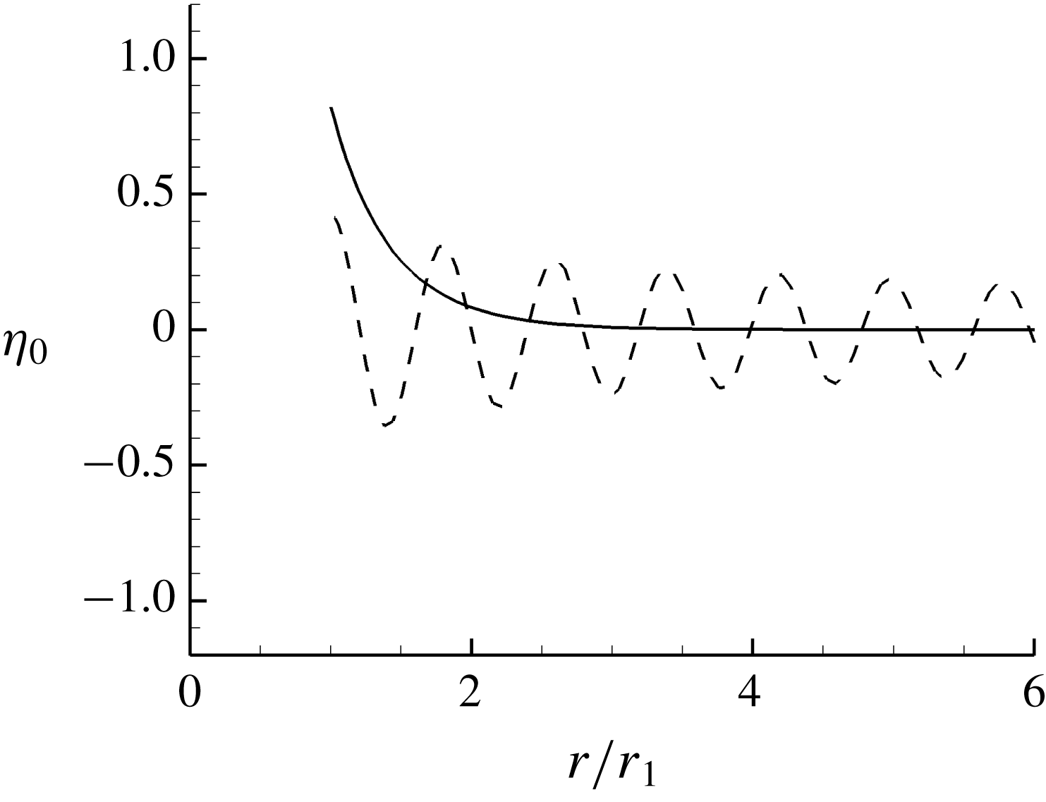
One notes that the evanescent component in this case is not exactly zero (but negligibly small) since the functions $\text{e}^{\unicode[STIX]{x1D707}_{0}\unicode[STIX]{x1D709}}$ and $[k(1-\unicode[STIX]{x1D706}k^{2})\sin k\unicode[STIX]{x1D709}+4(1+\unicode[STIX]{x1D706})\cos k\unicode[STIX]{x1D709}]$ are not exactly orthogonal for $\unicode[STIX]{x1D709}\in (-\infty ,0]$ (Rhodes-Robinson Reference Rhodes-Robinson1971). Figure 4 displays sample axial-symmetric evanescent and propagating wave profiles generated with $f(\unicode[STIX]{x1D709})$ given by (4.23) and (4.25).

Figure 4.

Wave profiles of axial-symmetric outgoing waves generated by the swelling–contraction oscillation of a vertical circular cylinder with the wave-maker function given by (4.23) with $\unicode[STIX]{x1D707}_{p}=0.5$ (——) and (4.25) (– – –). ( $k_{0}r_{1}=3.98$ .)

4.3 Evolution equation for a cross-wave

Substituting the perturbation expansions, (4.2) and (4.3), into the Lagrangian (4.1), taking average over the fast time $\unicode[STIX]{x1D703}=\unicode[STIX]{x1D714}_{0}t$ , and keeping the terms related to the cross-wave, we obtain the (dimensionless) average Lagrangian

(4.27) $$\begin{eqnarray}\displaystyle \overline{L}\equiv \frac{k_{0}^{5}}{\unicode[STIX]{x1D714}_{0}^{2}}\langle 2L\rangle =(\overline{L}_{11}+\overline{L}_{011})\unicode[STIX]{x1D707}^{2}\unicode[STIX]{x1D700}+O(\unicode[STIX]{x1D707}^{3}\unicode[STIX]{x1D700},\unicode[STIX]{x1D707}^{2}\unicode[STIX]{x1D700}^{2}), & & \displaystyle\end{eqnarray}$$

where $\overline{L}_{11}$ is a quadratic function of the cross-wave amplitude, and $\overline{L}_{011}$ depends linearly on the axial-symmetric wave amplitude and quadratically on the cross-wave amplitude. $\overline{L}_{011}$ accounts for the subharmonic (quadratic) interaction of the axial-symmetric wave and the radial cross-wave. The detailed derivation and lengthy expressions for $\overline{L}_{11}$ and $\overline{L}_{011}$ are summarized in appendices B and C, respectively.

Upon invoking Hamilton’s principle,

(4.28) $$\begin{eqnarray}\displaystyle \unicode[STIX]{x1D6FF}\int \overline{L}\,\text{d}\unicode[STIX]{x1D70F}=0 & & \displaystyle\end{eqnarray}$$

we obtain the evolution equation for the amplitude of a radial cross-wave mode of azimuthal wavenumber $m$ :

(4.29) $$\begin{eqnarray}\displaystyle A_{\unicode[STIX]{x1D70F}}+\unicode[STIX]{x1D6FE}^{\prime }A_{R}+\unicode[STIX]{x1D6FE}_{P_{s}}A^{\ast }-\text{i}\unicode[STIX]{x1D700}\unicode[STIX]{x1D6FE}_{v}A_{RR}=0, & & \displaystyle\end{eqnarray}$$

with the boundary conditions at the waterline ( $R=R_{1}$ ) and far field ( $R=R_{2}$ ) given by

(4.30) $$\begin{eqnarray}\displaystyle \unicode[STIX]{x1D6FE}_{4}A_{R}+P_{W}A^{\ast }+\frac{D_{1}^{\prime }}{\unicode[STIX]{x1D700}}A=0,\quad R=R_{1} & & \displaystyle\end{eqnarray}$$

and

(4.31) $$\begin{eqnarray}\displaystyle \unicode[STIX]{x1D6FE}_{4}A_{R}+\text{i}\frac{\text{Im}\{\unicode[STIX]{x1D6FE}_{1}\}}{2\unicode[STIX]{x1D700}}A=0,\quad R=R_{2}\rightarrow \infty . & & \displaystyle\end{eqnarray}$$

The coefficients in (4.29), (4.30) and (4.31) are functions of $\bar{\unicode[STIX]{x1D711}}_{m}$ , $\bar{\unicode[STIX]{x1D702}}_{m}$ , $\unicode[STIX]{x1D711}_{0}$ and $\unicode[STIX]{x1D702}_{0}$ (derived in §§ 4.1 and 4.2) and take the form

(4.32a-c ) $$\begin{eqnarray}\displaystyle \unicode[STIX]{x1D6FE}^{\prime }=\frac{\unicode[STIX]{x1D6FE}_{1}-\unicode[STIX]{x1D6FE}_{1}^{\ast }}{\unicode[STIX]{x1D71B}_{2}-\unicode[STIX]{x1D71B}_{2}^{\ast }}+\frac{\unicode[STIX]{x1D6FE}_{4\unicode[STIX]{x1D70C}}}{\unicode[STIX]{x1D71B}_{2}-\unicode[STIX]{x1D71B}_{2}^{\ast }},\quad \unicode[STIX]{x1D6FE}_{P_{s}}=\frac{P_{s}}{\unicode[STIX]{x1D71B}_{2}-\unicode[STIX]{x1D71B}_{2}^{\ast }},\quad \unicode[STIX]{x1D6FE}_{v}=\frac{\unicode[STIX]{x1D6FE}_{4}}{\text{Im}\{\unicode[STIX]{x1D71B}_{2}\}}, & & \displaystyle\end{eqnarray}$$

(4.33) $$\begin{eqnarray}\displaystyle & \displaystyle \unicode[STIX]{x1D6FE}_{1}=\int _{-\infty }^{0}\left(\unicode[STIX]{x1D70C}\overline{\unicode[STIX]{x1D711}}_{m}^{\ast }\overline{\unicode[STIX]{x1D711}}_{m\unicode[STIX]{x1D70C}}+\frac{1}{2}\overline{\unicode[STIX]{x1D711}}_{m}^{\ast }\overline{\unicode[STIX]{x1D711}}_{m}\right)\text{d}\unicode[STIX]{x1D709}+\left(\frac{\unicode[STIX]{x1D706}}{1+\unicode[STIX]{x1D706}}\right)\left(\unicode[STIX]{x1D70C}\overline{\unicode[STIX]{x1D702}}_{m}^{\ast }\overline{\unicode[STIX]{x1D702}}_{m\unicode[STIX]{x1D70C}}+\frac{1}{2}\overline{\unicode[STIX]{x1D702}}_{m}^{\ast }\overline{\unicode[STIX]{x1D702}}_{m}\right), & \displaystyle\end{eqnarray}$$

(4.34) $$\begin{eqnarray}\displaystyle & \displaystyle \unicode[STIX]{x1D6FE}_{4}=\int _{-\infty }^{0}\unicode[STIX]{x1D70C}\overline{\unicode[STIX]{x1D711}}_{m}^{\ast }\overline{\unicode[STIX]{x1D711}}_{m}\,\text{d}\unicode[STIX]{x1D709}+\left(\frac{\unicode[STIX]{x1D706}}{1+\unicode[STIX]{x1D706}}\right)\unicode[STIX]{x1D70C}\overline{\unicode[STIX]{x1D702}}_{m}^{\ast }\overline{\unicode[STIX]{x1D702}}_{m}, & \displaystyle\end{eqnarray}$$

(4.35) $$\begin{eqnarray}\displaystyle & \displaystyle D_{1}^{\prime }=\frac{1}{2}\left(\frac{\unicode[STIX]{x1D706}}{1+\unicode[STIX]{x1D706}}\right)\text{Re}\{\unicode[STIX]{x1D70C}_{1}\overline{\unicode[STIX]{x1D702}}_{m}^{\ast }\overline{\unicode[STIX]{x1D702}}_{m\unicode[STIX]{x1D70C}}\}+\frac{\text{i}}{2}\text{Im}\{\unicode[STIX]{x1D6FE}_{1}\}, & \displaystyle\end{eqnarray}$$

where $\unicode[STIX]{x1D71B}_{2}=\unicode[STIX]{x1D70C}\overline{\unicode[STIX]{x1D711}}_{m}^{\ast }\overline{\unicode[STIX]{x1D702}}_{m}/2$ and

(4.36) $$\begin{eqnarray}\displaystyle P_{s} & = & \displaystyle \frac{\unicode[STIX]{x1D70C}}{4} (\!-\overline{\unicode[STIX]{x1D711}}_{m\unicode[STIX]{x1D709}\unicode[STIX]{x1D709}}^{\ast }\overline{\unicode[STIX]{x1D711}}_{m}^{\ast }\unicode[STIX]{x1D702}_{0}-\overline{\unicode[STIX]{x1D711}}_{m}^{\ast }\overline{\unicode[STIX]{x1D702}}_{m}^{\ast }\unicode[STIX]{x1D711}_{0\unicode[STIX]{x1D709}\unicode[STIX]{x1D709}}+\overline{\unicode[STIX]{x1D711}}_{m\unicode[STIX]{x1D709}}^{\ast }\overline{\unicode[STIX]{x1D702}}_{m}^{\ast }\unicode[STIX]{x1D711}_{0\unicode[STIX]{x1D709}}+\overline{\unicode[STIX]{x1D711}}_{m}^{\ast }\overline{\unicode[STIX]{x1D702}}_{m\unicode[STIX]{x1D70C}}^{\ast }\unicode[STIX]{x1D711}_{0\unicode[STIX]{x1D70C}}+\overline{\unicode[STIX]{x1D711}}_{m}^{\ast }\overline{\unicode[STIX]{x1D711}}_{m\unicode[STIX]{x1D70C}}^{\ast }\unicode[STIX]{x1D702}_{0\unicode[STIX]{x1D70C}}\nonumber\\ \displaystyle & & \displaystyle +\,\overline{\unicode[STIX]{x1D711}}_{m\unicode[STIX]{x1D709}}^{\ast }\overline{\unicode[STIX]{x1D702}}_{m}^{\ast }\unicode[STIX]{x1D711}_{0\unicode[STIX]{x1D709}}+\overline{\unicode[STIX]{x1D711}}_{m\unicode[STIX]{x1D709}}^{\ast }\overline{\unicode[STIX]{x1D711}}_{m\unicode[STIX]{x1D709}}^{\ast }\unicode[STIX]{x1D702}_{0}\! ),\end{eqnarray}$$

(4.37) $$\begin{eqnarray}\displaystyle P_{W} & = & \displaystyle \frac{\text{i}\unicode[STIX]{x1D70C}_{1}}{4}\left[\overline{\unicode[STIX]{x1D711}}_{m\unicode[STIX]{x1D709}}^{\ast }\overline{\unicode[STIX]{x1D711}}_{m}^{\ast }+\left(\frac{1}{1+\unicode[STIX]{x1D706}}-\unicode[STIX]{x1D706}\frac{m^{2}}{\unicode[STIX]{x1D70C}_{1}^{2}}\right)\overline{\unicode[STIX]{x1D702}}_{m}^{\ast }\overline{\unicode[STIX]{x1D702}}_{m}^{\ast }+\unicode[STIX]{x1D706}\right]_{\unicode[STIX]{x1D70C}=\unicode[STIX]{x1D70C}_{1},\unicode[STIX]{x1D709}=0}f(0)\nonumber\\ \displaystyle & & \displaystyle +\,\frac{\text{i}\unicode[STIX]{x1D70C}_{1}}{4}\int _{0}^{\infty }[\overline{\unicode[STIX]{x1D711}}_{m}^{\ast }\overline{\unicode[STIX]{x1D711}}_{m\unicode[STIX]{x1D70C}\unicode[STIX]{x1D70C}}^{\ast }f(\unicode[STIX]{x1D709})-\overline{\unicode[STIX]{x1D711}}_{m}^{\ast }\overline{\unicode[STIX]{x1D711}}_{m\unicode[STIX]{x1D709}}^{\ast }f_{\unicode[STIX]{x1D709}}(\unicode[STIX]{x1D709})]_{\unicode[STIX]{x1D70C}=\unicode[STIX]{x1D70C}_{1}}\,\text{d}\unicode[STIX]{x1D709}.\end{eqnarray}$$

The detailed derivation of the evolution equation (4.29) and associated boundary conditions (4.30) and (4.31) is described in appendix D. One notes that the boundary condition (4.30) follows directly from the application of Hamilton’s principle. It is not straightforward to derive this boundary condition from physical arguments. This is indeed the reason why we adopt the average Lagrangian method to derive the evolution equation for the radial cross-wave.

The coefficients $\unicode[STIX]{x1D6FE}_{P_{s}}$ and $P_{W}$ are associated with the subharmonic interaction of the cross-wave and axial-symmetric wave. The two terms associated with them in (4.29) and (4.30) represent energy input from the base axial-symmetric wave to cause the growth of the cross-wave. The term associated with $D_{1}^{\prime }$ in (4.30) represents the energy dissipation in the evolution of the cross-wave. In order for the cross-wave to grow, the energy input from the base axial-symmetric wave must be sufficiently large to overcome the dissipation effect. This implies that there must exist a non-trivial threshold value of the steepness of the axial-symmetric wave beyond which the axial-symmetric wave can provide sufficient energy to substantiate the growth of the cross-wave. Within the threshold value, the axial-symmetric wave is unable to supply enough energy to overcome the dissipation effect and enable the cross-wave growth. As shown in (4.35), $D_{1}^{\prime }$ contains two terms, one of which is real while the other is purely imaginary. The real term represents the dissipation associated with the work done by the surface tension force at the waterline. The imaginary term represents the dissipation due to energy radiation (to the far field) in the cross-wave’s outgoing propagation. It is worth noting that in the work of Becker & Miles (Reference Becker and Miles1992), the cross-wave considered is a standing wave with zero radial slope of the wave profile at the waterline, for which there is no dissipation effect (as $D_{1}^{\prime }=0$ ) at the leading order in the cross-wave interaction with the axial-symmetric wave. This leads to their result of a near-zero threshold value of the axial-symmetric wave amplitude for the cross-wave to grow.

5 Results for the vertical circular cylinder case

Starting with any specified small initial value of the progressive radial cross-wave amplitude $A(R,\unicode[STIX]{x1D70F}=0)$ , integration of the evolution equation (4.29) with respect to $\unicode[STIX]{x1D70F}$ and $R$ subject to the boundary conditions (4.30) and (4.31) gives the temporal–spatial variation of $A(R,\unicode[STIX]{x1D70F})$ due to the subharmonic resonant interaction of the cross-wave and base axial-symmetric progressive wave. Since the coefficients in (4.29) are spatially dependent, it is difficult to derive the analytic solution of $A(R,\unicode[STIX]{x1D70F})$ . We apply numerical integration to solve the initial-boundary-value problem for $A(R,\unicode[STIX]{x1D70F})$ . Specifically, we employ an implicit backward Euler scheme for the approximation of the time derivative and the second-order central difference for spatial derivatives in (4.29), (4.30) and (4.31). Through numerical convergence tests, we choose to use the temporal and spatial discretization $\unicode[STIX]{x0394}\unicode[STIX]{x1D70F}=0.01$ and $\unicode[STIX]{x0394}R=0.01$ and the domain size $R_{1}\leqslant R\leqslant R_{2}=30$ . With these numerical parameters, the numerical error in the solution of $A(R,\unicode[STIX]{x1D70F}=100)$ is within 1 %.

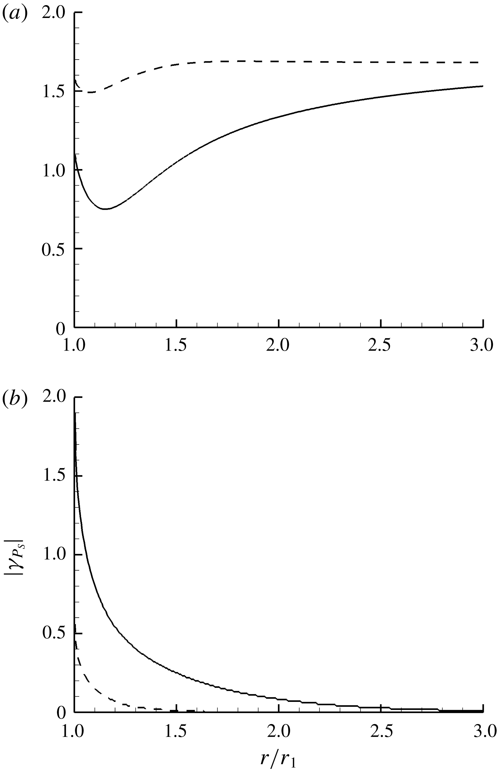
Figure 5 shows the spatial variations of the coefficients $\unicode[STIX]{x1D6FE}^{\prime }$ , $\unicode[STIX]{x1D6FE}_{v}$ and $\unicode[STIX]{x1D6FE}_{P_{s}}$ . The magnitudes of these coefficients vary rapidly near the body and asymptotically approach constants at the far field (for $R\gg 1$ ). Specifically, $\unicode[STIX]{x1D6FE}^{\prime }$ is complex near the body and becomes real at the far field while $\unicode[STIX]{x1D6FE}_{v}$ is always real positive. Both $|\unicode[STIX]{x1D6FE}^{\prime }|$ and $|\unicode[STIX]{x1D6FE}_{v}|$ approach the same constant $(1+3\unicode[STIX]{x1D706})/(1+\unicode[STIX]{x1D706})$ as $R\rightarrow \infty$ . The forcing coefficient $\unicode[STIX]{x1D6FE}_{P_{s}}$ is generally complex. The magnitude of $\unicode[STIX]{x1D6FE}_{P_{s}}$ decays rapidly with the distance from the waterline if the base axial-symmetric wave is dominated by the evanescent component. It is nearly constant if the axial-symmetric wave is dominated by the propagating component.

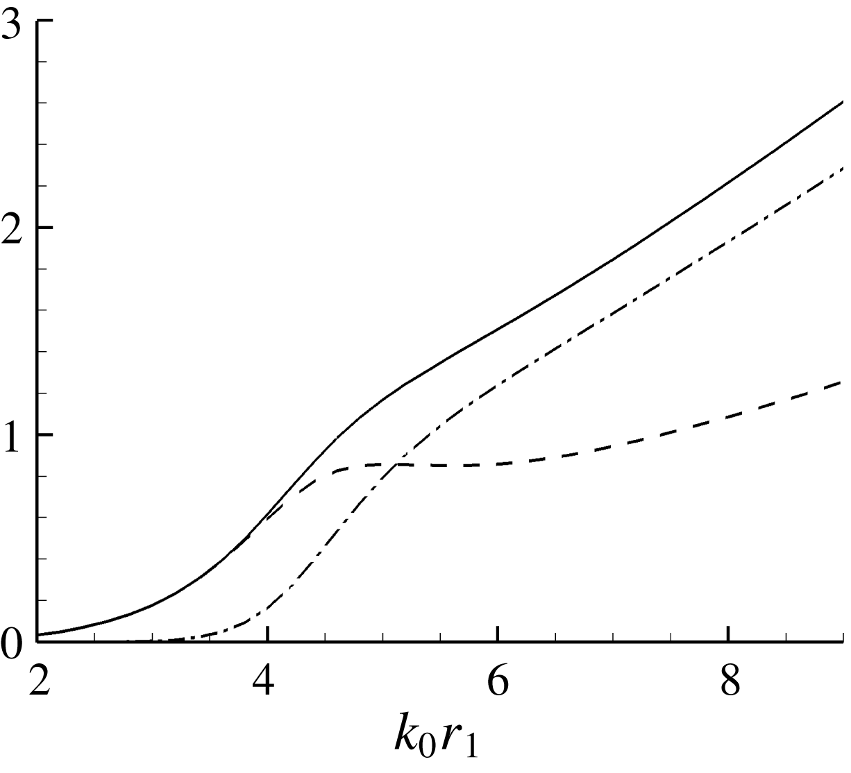
Figure 6 plots the damping coefficient $D_{1}^{\prime }$ and its real and imaginary parts for the radial cross-wave with azimuthal wavenumber $m=5$ as a function of cylinder radius $k_{0}r_{1}$ . It is seen that for $k_{0}r_{1}\ll m$ , $D_{1}^{\prime }$ is dominated by its real part, for which the dissipation is mainly due to energy loss to overcome the work done by the surface tension force at the waterline. For $k_{0}r_{1}\gg m$ , $D_{1}^{\prime }$ is dominated by its imaginary part, for which the dissipation is mainly due to wave radiation to the far field.

Figure 5.

Spatial variations of the coefficients $\unicode[STIX]{x1D6FE}^{\prime }$ , $\unicode[STIX]{x1D6FE}_{v}$ and $\unicode[STIX]{x1D6FE}_{P_{s}}$ for the subharmonic interaction of an axial-symmetric progressive wave and a progressive radial cross-wave with azimuthal wavenumber $m=5$ in the vertical circular cylinder case ( $k_{0}r_{1}=3.98$ ). The plotted curves are: (a) the module of $\unicode[STIX]{x1D6FE}^{\prime }$ (——) and $\unicode[STIX]{x1D6FE}_{v}$ (– – –); and (b) the module of $\unicode[STIX]{x1D6FE}_{P_{s}}$ for the axial-symmetric evanescent wave with wave-maker function (4.23) with $\unicode[STIX]{x1D707}_{p}=0.5$ (——) and the axial-symmetric propagating wave with wave-maker function (4.25) (– – –).

Figure 6.

The damping coefficient $D_{1}^{\prime }$ of the radial cross-wave with azimuthal wavenumber $m=5$ as a function of the radius of the vertical circular cylinder $k_{0}r_{1}$ . The plotted curves represent $|D_{1}^{\prime }|$ (——), $-\text{Re}\{D_{1}^{\prime }\}$ (– – –), and $\text{Im}\{D_{1}^{\prime }\}$ (— ⋅ —).

To illustrate how the cross-wave develops due to the subharmonic resonant interaction with the axial-symmetric wave, we first consider that the base axial-symmetric wave contains the evanescent component only, which is generated with the wave-maker function given by (4.23). For numerical illustration, we choose the wavenumber of the evanescent wave component to be $\unicode[STIX]{x1D707}_{p}=0.5$ .

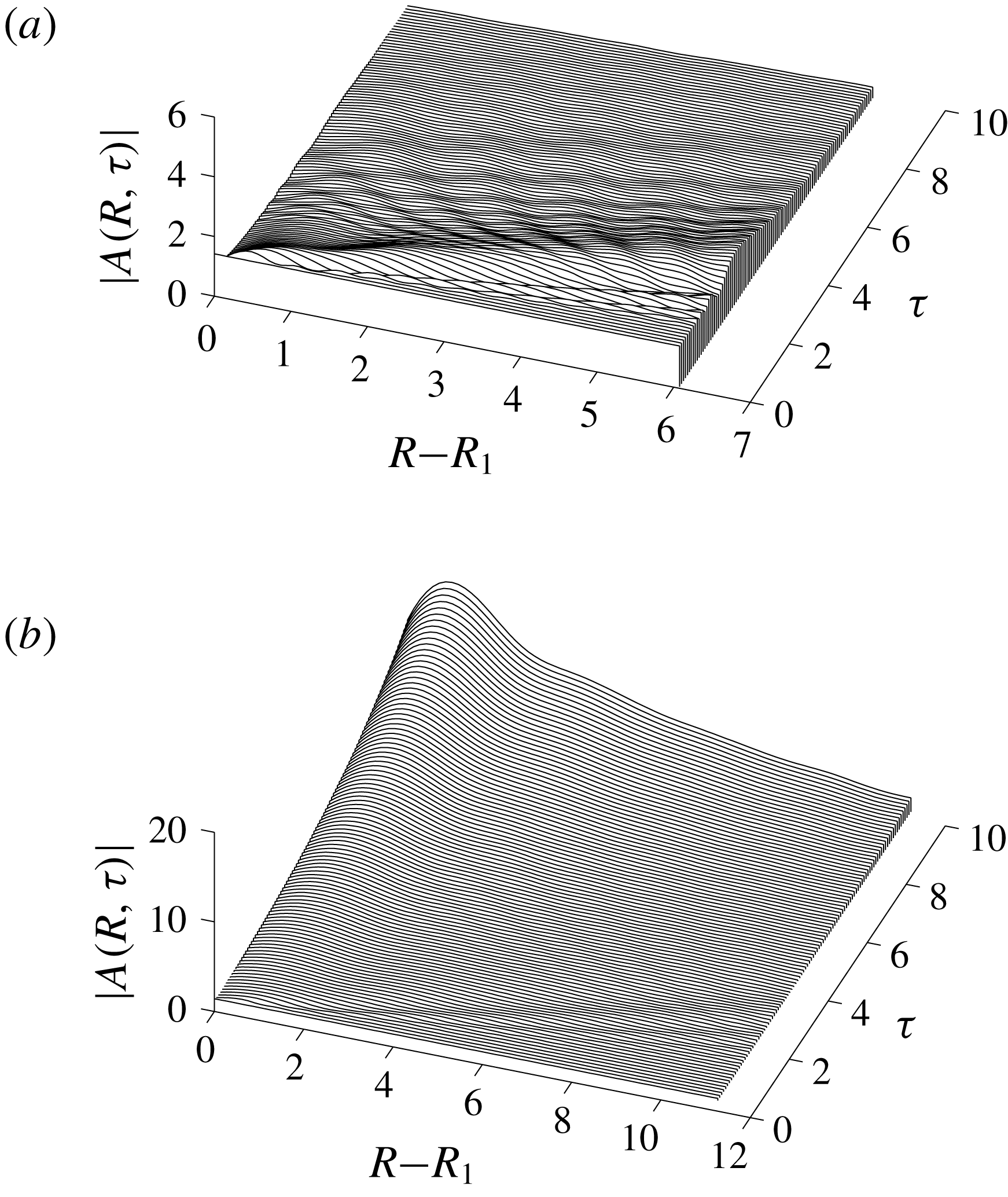
Figure 7(a,b) displays the spatial–temporal evolution of the amplitude $|A(R,\unicode[STIX]{x1D70F})|$ of the cross-wave with azimuthal wavenumber $m=5$ for two different oscillation amplitudes of the cylinder $\unicode[STIX]{x1D700}=0.2$ and 0.37. The radius of the cylinder is $k_{0}r_{1}=3.98$ . For the relatively small ring wave (with $\unicode[STIX]{x1D700}=0.2$ ) case, $A(R,\unicode[STIX]{x1D70F})$ actually decays from its initial value $A(R,0)=1-\text{i}$ (which is arbitrarily assigned). For the relatively large ring wave (with $\unicode[STIX]{x1D700}=0.37$ ) case, $A(R,\unicode[STIX]{x1D70F})$ grows continuously with time by taking energy from the forced ring wave. 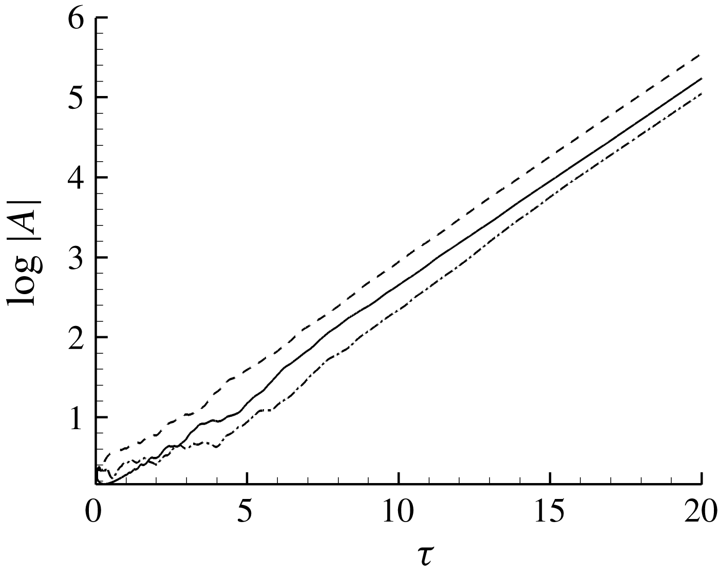The growth of $A(R,\unicode[STIX]{x1D70F})$ starts at the waterline and then spreads to the far field gradually. Figure 8 compares the time histories of $A(R,\unicode[STIX]{x1D70F})$ at three different spatial locations. The comparison shows that after the initial transient adjustment, $A(R,\unicode[STIX]{x1D70F})$ at different locations all grow exponentially with time, like $\text{e}^{\unicode[STIX]{x1D70E}\unicode[STIX]{x1D70F}}$ , and achieve the same growth rate $\unicode[STIX]{x1D70E}$ . We thus use the growth rate of $A(R,\unicode[STIX]{x1D70F})$ at the waterline ( $R_{1}=k_{0}r_{1}$ ) to represent the growth rate of the whole cross-wave in the following discussion.

Figure 7.

Waterfall plot of the spatial–temporal evolution of the cross-wave amplitude $|A(R,\unicode[STIX]{x1D70F})|$ for the vertical circular cylinder case. The plots are for the oscillation amplitude of the cylinder (a) $\unicode[STIX]{x1D700}=0.20$ and (b) $\unicode[STIX]{x1D700}=0.37$ . The azimuthal wavenumber of radial cross-wave $m=5$ and cylinder radius $k_{0}r_{1}=3.98$ .

Figure 8.

Time history of the amplitude $|A|$ of the radial cross-wave with azimuthal wavenumber $m=5$ at three different locations $R_{1}=2\unicode[STIX]{x1D700}k_{0}r_{1}$ (waterline) (——), $R=R_{1}+1$ (– – –), and $R=R_{1}+2$ (— ⋅ —) in subharmonic interaction with the forced axial-symmetric wave. The vertical circular cylinder has an oscillation amplitude $\unicode[STIX]{x1D700}=0.37$ and a radius of $k_{0}r_{1}=3.98$ .

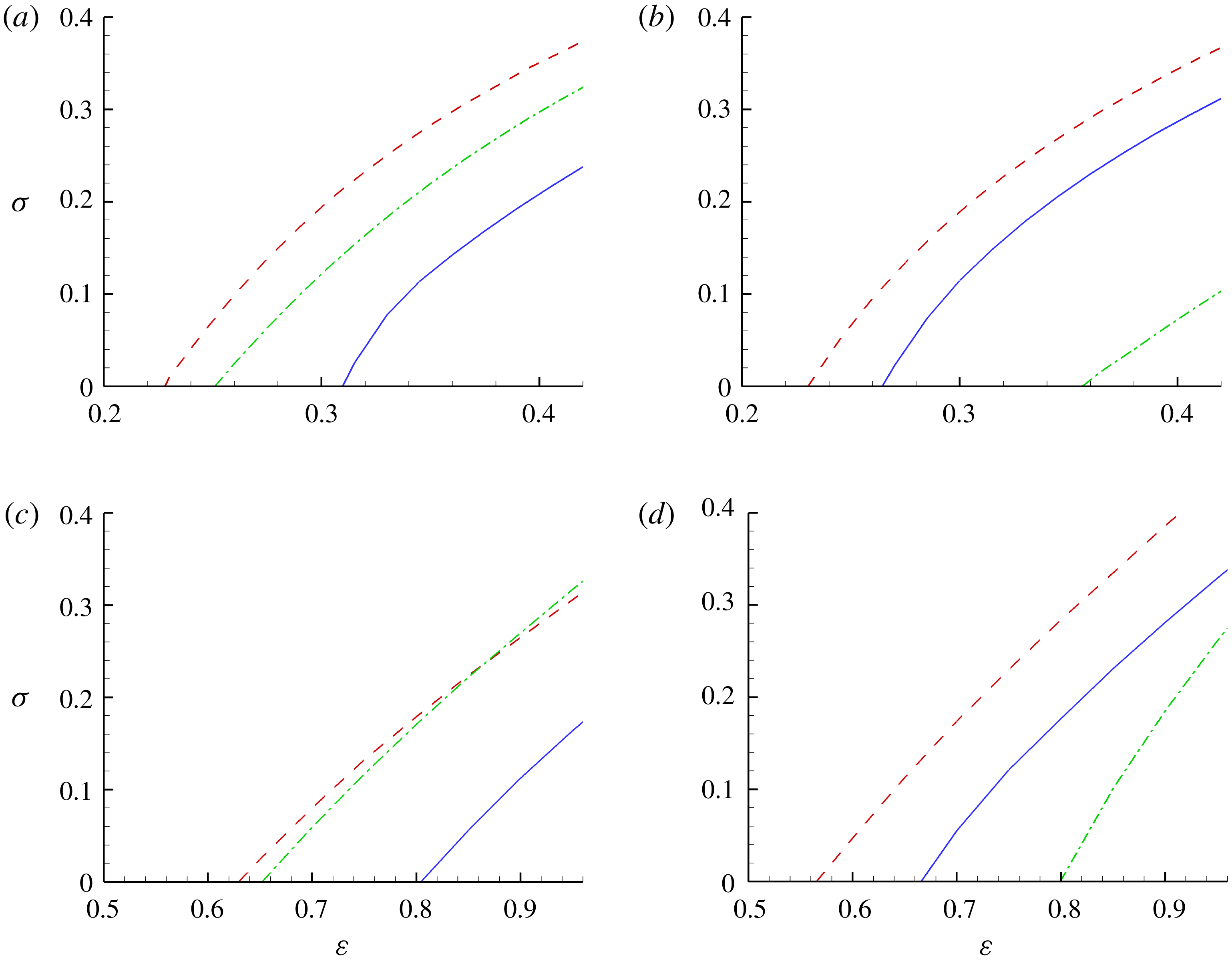
Figure 9 shows the growth rate $\unicode[STIX]{x1D70E}$ of the cross-wave mode as a function of cylinder oscillation amplitude $\unicode[STIX]{x1D700}$ for different azimuthal wavenumber $m$ and oscillation frequency (or cylinder radius) $k_{0}r_{1}$ . Both evanescent and propagating components of the base axial-symmetric wave can cause the cross-waves to grow. The threshold value of the motion amplitude $\unicode[STIX]{x1D700}_{c}$ for the evanescent wave component ( $\unicode[STIX]{x1D700}_{c}\sim 0.2$ ) is much smaller than that for the propagating wave component ( $\unicode[STIX]{x1D700}_{c}\sim 0.6$ ).

Figure 9.

Growth rate $\unicode[STIX]{x1D70E}$ of the cross-wave as a function of cylinder oscillation amplitude $\unicode[STIX]{x1D700}$ for different azimuthal wavenumber $m$ and oscillation frequency (or cylinder radius) $k_{0}r_{1}$ . The plotted curves are for $m=3$ (——), $m=4$ (– – –), $m=5$ (— ⋅ —). (a,b) The case where the forced axial-symmetric wave contains an evanescent component only which is generated using the wave-maker function given by (4.23) with $\unicode[STIX]{x1D707}_{p}=0.5$ at oscillation frequency $k_{0}r_{1}=3.98$ and 3.40, respectively. (c,d) The case where the forced axial-symmetric wave contains the propagating component which is generated using the wave-maker function given by (4.25) at oscillation frequency $k_{0}r_{1}=3.98$ and 3.40, respectively.

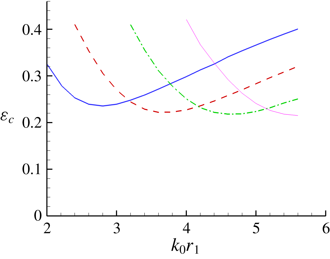
Figure 10 shows the threshold value of cylinder oscillation amplitude $\unicode[STIX]{x1D700}_{c}$ , at which the growth rate of the cross-wave equals zero, as a function of cylinder radius or oscillation frequency ( $k_{0}r_{1}$ ) for azimuthal wavenumber $m=3$ , 4, 5 and 6. If $\unicode[STIX]{x1D700}>\unicode[STIX]{x1D700}_{c}$ (or ${<}\unicode[STIX]{x1D700}_{c}$ ), the cross-wave will grow (or decay) with time as the energy input from the axial-symmetric wave is sufficient (or insufficient) to overcome the damping effect of the cross-wave. It is seen that $\unicode[STIX]{x1D700}_{c}$ shows a convex variation with $k_{0}r_{1}$ for all $m$ . This feature of the solution is consistent with the general fact that the wave-making capability of an oscillating body tends to vanish at very low and high frequencies. The maximum wave making capability, corresponding to the minimum $\unicode[STIX]{x1D700}_{c}$ for a given $m$ , is thus achieved at some intermediate frequency. The results in figure 10 indicate that the minimum value of $\unicode[STIX]{x1D700}_{c}$ is achieved by the cross-wave mode with azimuthal wavenumber $m^{\ast }\simeq 1.2k_{0}r_{1}$ .

Figure 10.

Threshold value $\unicode[STIX]{x1D700}_{c}$ of the cylinder oscillation amplitude, at which the cross-wave mode has a zero growth rate, as a function of vertical cylinder radius $k_{0}r_{1}$ for different azimuthal wavenumber $m$ of the cross-waves. The plotted curves are for $m=3$ (——, blue), $m=4$ (– – –), $m=5$ (— ⋅ —), and $m=6$ (——, pink). The axial-symmetric wave contains an evanescent component generated with the wave-maker function given by (4.23) with $\unicode[STIX]{x1D707}_{p}=0.5$ .

We remark that since only the quadratic interaction between the base ring wave and the radial cross-wave are considered, the present analysis is valid for the steepness of the unstable cross-wave ( $\unicode[STIX]{x1D707}$ ) growing up to the value comparable to that of the base wave ( $\unicode[STIX]{x1D700}$ ), beyond which the higher-order interactions needs to be accounted for in the analysis.

6 Results for a half-submerged vertically oscillating sphere

We apply the analysis for a vertical circular cylinder in the preceding section to investigate the experimental case of TIO. In TIO’s experiment, a half-submerged sphere is forced to oscillate up and down periodically to generate outgoing waves. When the oscillation amplitude is small, the generated wave is an axial-symmetric ring-type progressive wave, while when the oscillation amplitude is increased to beyond a threshold value, apparent asymmetric outgoing waves appear. We shall investigate the role of subharmonic resonant interactions of the forced propagating ring wave with its subharmonic radial cross-waves in the development of asymmetric wave patterns observed in TIO’s experiment.

We express the (normalized) displacement of the centre of the sphere undergoing a periodic vertical oscillation in the form

(6.1) $$\begin{eqnarray}\displaystyle \unicode[STIX]{x1D6EF}=-\unicode[STIX]{x1D700}f(\unicode[STIX]{x1D709})\sin 2\unicode[STIX]{x1D714}_{0}t, & & \displaystyle\end{eqnarray}$$

where $\unicode[STIX]{x1D700}=k_{0}a$ with $a$ being the dimensional amplitude of the oscillation. Since the oscillation frequency in the experiment is quite high ( $k_{0}r_{1}\gg 1$ , where $r_{1}$ is the radius of the sphere), we approximate the solution of the forced wave motion as (Becker & Miles Reference Becker and Miles1992)

(6.2) $$\begin{eqnarray}\displaystyle \unicode[STIX]{x1D711}_{0}=\unicode[STIX]{x1D70C}_{1}^{3}\unicode[STIX]{x1D709}(\unicode[STIX]{x1D70C}^{2}+\unicode[STIX]{x1D709}^{2})^{-3/2}. & & \displaystyle\end{eqnarray}$$

Let the radial velocity in the horizontal plane of this flow be identical to that of a vertical circular cylinder at $\unicode[STIX]{x1D70C}=\unicode[STIX]{x1D70C}_{1}=k_{0}r_{1}$ . We then obtain an equivalent wave-maker function $f(\unicode[STIX]{x1D709})$ for the vertical circular cylinder

(6.3) $$\begin{eqnarray}\displaystyle f(\unicode[STIX]{x1D709})=-{\textstyle \frac{3}{2}}\unicode[STIX]{x1D70C}_{1}^{4}\unicode[STIX]{x1D709}(\unicode[STIX]{x1D70C}_{1}+\unicode[STIX]{x1D709}^{2})^{-5/2}. & & \displaystyle\end{eqnarray}$$

Using this $f(\unicode[STIX]{x1D709})$ , we obtain the solution of the propagating wave component from (4.20). We could add this contribution to (6.2) to further improve the accuracy of the forced wave solution. For $k_{0}r_{1}\gg 1$ , we also assume that the cross-wave modes of the sphere are identical to those of a vertical circular cylinder of the same radius as the sphere. With this information, we can evaluate the growth rate of radial cross-waves and the threshold value of sphere oscillation amplitude for radial cross-waves to be formed.

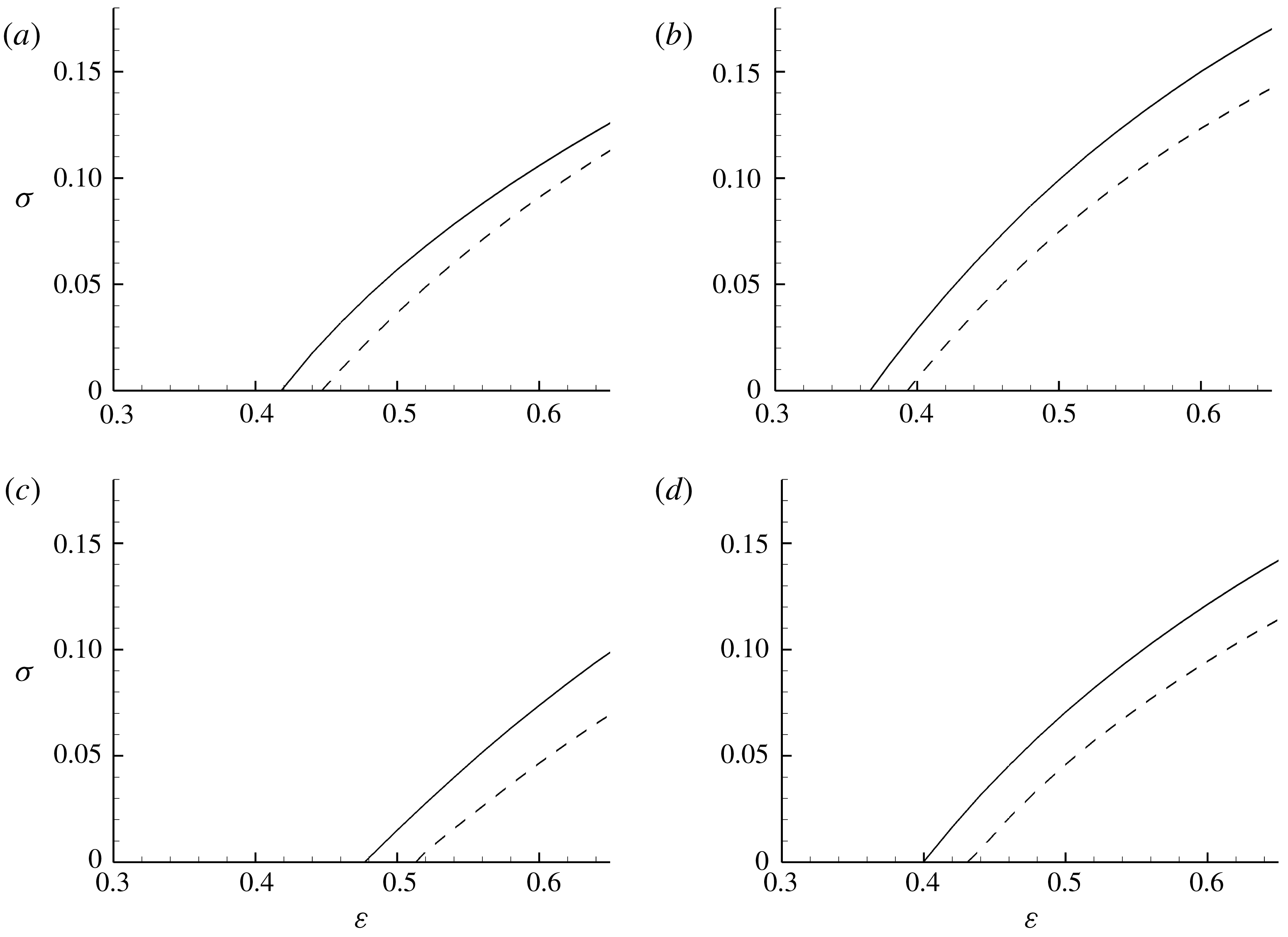
Figures 11(a), 11(b) and 11(c) display the growth rate of cross-wave modes with azimuthal wavenumber $m=5$ , 4 and 3, respectively, at the frequency $k_{0}r_{1}=3.98$ . The growth rate increases with the oscillation amplitude $\unicode[STIX]{x1D700}$ , but the dependence on $\unicode[STIX]{x1D700}$ is not linear due to the existence of the $D_{1}^{\prime }$ term in the waterline boundary condition. Figure 11(d) shows the growth rate for the case of $k_{0}r_{1}=3.37$ and $m=4$ , which has a similar behaviour to the $k_{0}r_{1}=3.98$ , $m=4$ case. In order to evaluate the relative importance of evanescent wave component versus propagating wave component, the solution obtained with both evanescent and propagating components included is compared, in these figures, with that including the evanescent component only. It is seen that the inclusion of propagating wave component provides less than 10 % contribution to the growth rate. The evanescent wave component plays a dominant role in causing the growth of cross-waves in TIO’s experiment case.

Figure 11.

Theoretically predicted initial growth rate of radial cross-waves, in TIO’s experimental case, as a function of sphere oscillation amplitude $\unicode[STIX]{x1D700}$ : (a) frequency $k_{0}r_{1}=3.98$ and azimuthal wavenumber $m=5$ ; (b) $k_{0}r_{1}=3.98$ , $m=4$ ; (c) $k_{0}r_{1}=3.98$ , $m=3$ ; and (d) $k_{0}r_{1}=3.37$ , $m=4$ . The plotted curves represent the results obtained including both evanescent and propagating wave components (——) and the evanescent wave component only (– – –) in the forced ring wave field.

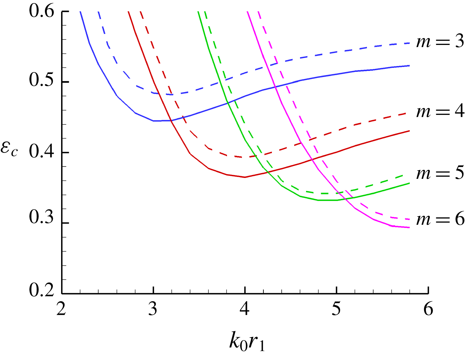
Figure 12 shows the threshold value of $\unicode[STIX]{x1D700}$ , beyond which the cross-wave is developed, for different frequency $k_{0}r_{1}$ and cross-wave azimuthal wavenumber $m$ . The characteristic behaviour of the threshold value in the case of vertical sphere oscillation is similar to the vertical circular cylinder case. The threshold curve for each azimuthal wavenumber has a minimum value roughly at $m^{\ast }\sim 1.2k_{0}r_{1}$ .

Figure 12.

Theoretically predicted threshold value of sphere vertical oscillation amplitude, in TIO’s experimental case, as a function of frequency $k_{0}r_{1}$ for different cross-wave azimuthal wavenumber $m$ . The curves for threshold value including both evanescent and propagating wave components in the forced ring wave field are for $m=3$ (——, blue), $m=4$ (——, red), $m=5$ (——, green), and $m=6$ (——, pink). The curves for threshold value considering evanescent wave component only in the forced ring wave field are for $m=3$ (– – –, blue), $m=4$ (– – –, red), $m=5$ (– – –, green), and $m=6$ (– – –, pink).

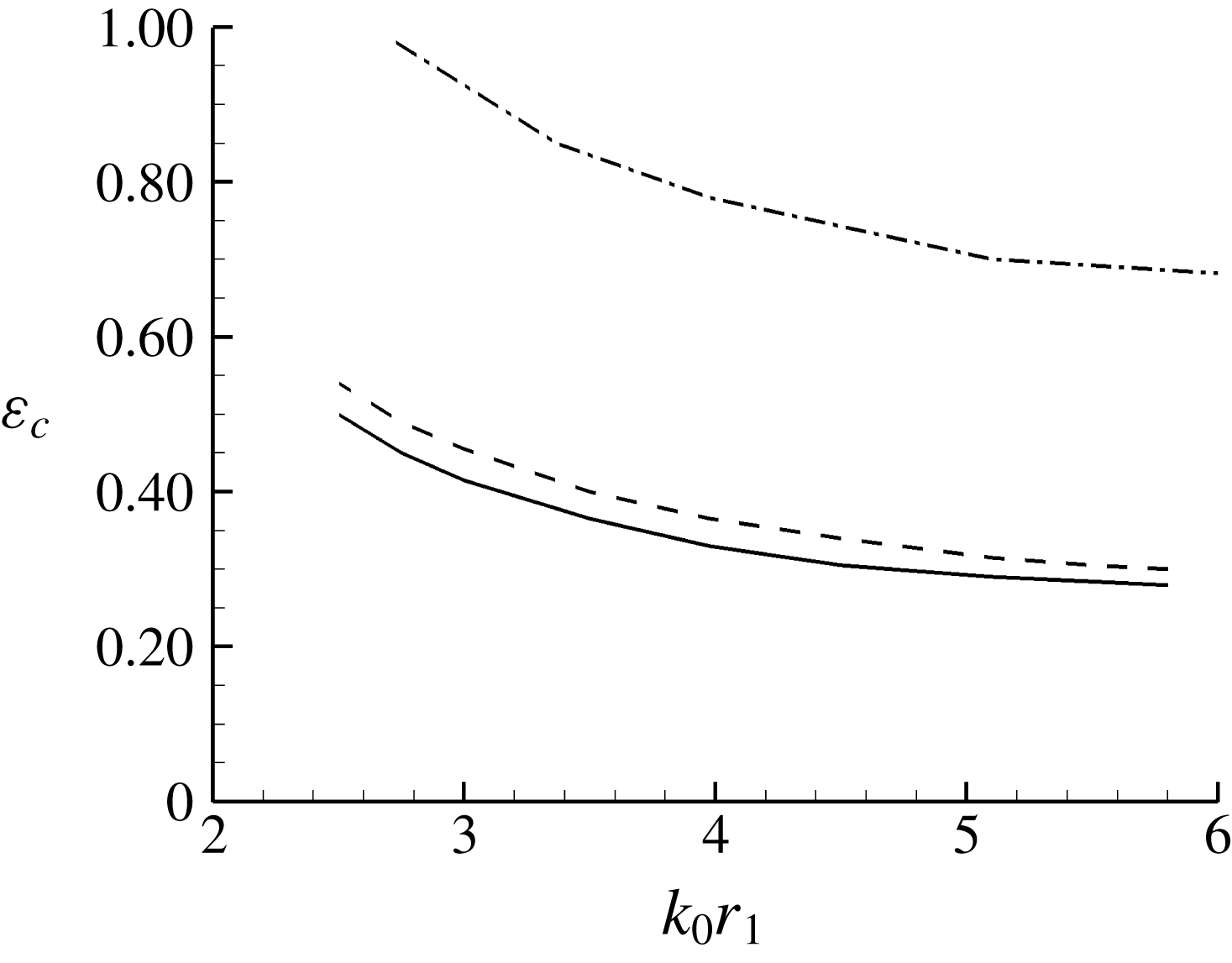
Figure 13 presents the result of overall threshold value $\unicode[STIX]{x1D700}_{c}$ as a function of $k_{0}r_{1}$ . TIO’s experimental data are also shown for comparison. The present theoretical solution of $\unicode[STIX]{x1D700}_{c}$ has the same trend of variation that $\unicode[STIX]{x1D700}_{c}$ is inversely proportional to $k_{0}r_{1}$ . The theoretically predicted $\unicode[STIX]{x1D700}_{c}$ is about 50 % smaller than TIO’s experimental data. We believe that the difference in $\unicode[STIX]{x1D700}_{c}$ between the theoretical prediction and the experimental data could be due to the neglect of nonlinear effects on the forced base axial-symmetric progressive wave and viscous damping effect (Miles 1967) in the present analysis. We are investigating these effects by the use of direct nonlinear numerical simulations, which will be published in a separate work.

Figure 13.

Comparison of overall threshold value of $\unicode[STIX]{x1D700}_{c}$ for different $k_{0}r_{1}$ between the present theoretical prediction and TIO’s experimental data. The plotted curves represent the theoretical solutions including both evanescent and propagating wave components (——) or the evanescent wave component only (– – –) in the forced axial-symmetric progressive wave field, and TIO’s experimental data (— ⋅ —).