2.1. Surrogate modelling of RDC

The structure of a typical RDC is illustrated in figure 1(a). The injector, situated at the head of the combustor, allowed the entry of fuel and oxidizer into the annular combustor. Within this combustor, a detonation wave traverses the circumferential path, consuming propellant to release heat, causing combustion products to expand towards the rear of the combustor and then exhaust through the nozzle. The combustion mode of the flow field can be observed by projecting the flow field to an observation plane parallel to the cross-section of annular channel.

On the observation plane, the gradients of the flow field in the radial direction and the curvature in the circumferential direction can be disregarded, since the diameter of a typical RDC is normally much larger than the radial distance between the inner and outer walls of the combustor, which causes the state variables of the flow field to vary slightly along the radial direction compared with their variations in other directions. Therefore, the flow field can be averaged out in radial direction, and the curvature of the annular channel can be disregarded. The circumferential dynamics on the observation plane capture dominant physical processes affecting the combustion modes. Owing to the average of radial gradients and neglection of the circumferential curvature, the circumferential dynamics can be modelled in a 1-D ‘unrolled’ domain with periodical boundary conditions to hold the periodicity in circumferential directions of the annular combustor.

However, the circumferential dynamics on the observation plane is an average of the axial dynamics in the combustor. The axial dynamics is dominant by the injection boundary and the exhaustion boundary on the flow field, by following a lumped parameter modelling scheme, these two boundaries can be averaged out as source terms $\boldsymbol{S}_{\textit{inj}}$ and $\boldsymbol{S}_{{ex}}$ to circumferential dynamics, which lead to the formulation of a generic 1-D surrogate model as follows:

(2.1) \begin{equation} \begin{array}{c} \boldsymbol{q}_{t}=\boldsymbol{f}(\boldsymbol{q})_{x}+\boldsymbol{S}_{{inj }}(\boldsymbol{q} ; \boldsymbol{c})-\boldsymbol{S}_{{ex}}(\boldsymbol{q} ; \boldsymbol{c})+\boldsymbol{S}(\boldsymbol{q} ; \boldsymbol{c}), \\[3pt] \boldsymbol{q}(x=0, t)=\boldsymbol{q}(x=L, t), \end{array} \end{equation}

where $\boldsymbol{q}$ = $[\rho , \rho u, E, \rho \lambda ]^{\textrm{T}}$ , $\boldsymbol{f}(\boldsymbol{q}) = -[\rho u, \rho u^2 + p, u(E + p), \rho u\lambda ]^{\textrm{T}}$ and $\rho , u, E, \lambda , p$ , respectively, represent the axially averaged density, circumferential velocity, total energy, reaction progress variable, pressure. $L$ is the average perimeter of the combustor. Here $\boldsymbol{S}_{\textit{inj}}$ , $\boldsymbol{S}_{{ex}}$ and $\boldsymbol{S}$ , respectively, represent injection submodel, exhaustion submodel and mixing-reaction submodel; these submodels are controlled by parameters $\boldsymbol{c}$ . The modelling procedure is schematically summarized in figure 1(a).

A different modelling approach can be applied to model $\boldsymbol{S}_{\textit{inj}}$ , $\boldsymbol{S}_{{ex}}$ and $\boldsymbol{S}$ . In this work, we consider one-step reaction between hydrogen and air, and the effect of viscosity and species diffusion are ignored. Here we choose the modelling results of Koch & Kutz (Reference Koch and Kutz2020),

(2.2) \begin{align} \boldsymbol{S}_{\textit{inj}}=\left (\begin{array}{c} \alpha A^+ H(p) \\[3pt] 0 \\[3pt] \frac {\alpha }{\gamma -1} A^+ H(p) \\[3pt] \alpha A^+ H(p) \lambda \end{array}\right ),\quad \boldsymbol{S}_{{ex}}=\left (\begin{array}{c} \alpha A^- \sqrt {p \rho } \\[3pt] 0 \\[3pt] \frac {\alpha }{\gamma -1} T A^- \sqrt {p \rho } \\[3pt] \alpha A^- \sqrt {p \rho } \lambda \end{array}\right ),\quad \boldsymbol{S}=\left (\begin{array}{c} 0 \\[3pt] 0 \\[3pt] \omega Q \\[3pt] \omega -\rho \lambda H(p) \beta \end{array}\right ),\nonumber\\[-2pt] \end{align}

where

(2.3) \begin{equation} \begin{array}{c} p=\rho R T, E=\dfrac {1}{\gamma -1} p+\dfrac {1}{2} \rho u^{2}, \alpha =\sqrt {\gamma }\left (\dfrac {2}{\gamma +1}\right )^{\frac {\gamma +1}{2(\gamma -1)}}, \\[6pt] H(p)=h(1-p)\left (1-h(p-Y) \dfrac {p-Y}{1-Y}\right ), Y=\left (1+\left (\dfrac {\gamma -1}{2}\right )\right )^{-\frac {\gamma }{\gamma -1}}, \\[8pt] \omega =Da \rho (1-\lambda ) \exp \left (\dfrac {E_{a}}{T_{V N}}-\dfrac {E_{a}}{T}\right ), \end{array} \end{equation}

where $R, \gamma , \omega$ , respectively, represent the gas constant, specific heat ratio of the mixture, rate of chemical reactions following Arrhenius in type with $E_{a}, Q$ respectively being activation energy and volumetric heat release associated with the propellant, pre-exponential factor and the activation energy. Here $T_{VN}$ is the von Neumann postshock temperature. All variables mentioned above are non-dimensionalized. The derivation of the submodels and non-dimensionalization method are briefly summarized in Appendix A.

Notably, these submodels contain a set of constant equation parameters $\boldsymbol{c} = [Da, \beta , A^+, A^-]$ which controls the physical processes, including injection ( $A^+$ ), mixing ( $\beta$ ), reaction ( $Da$ ) and exhaustion ( $A^-$ ). The definitions of these parameters and their physical interpretations are summarized in table 1.

Table 1.

Equation parameters of (2.2) and their impact on the physical processes.

By establishing the surrogate model (2.1) on the RDC, the detonation dynamics are modelled by dynamical balance between the energy input and output processes introduced by certain physical processes. Taking the control equation for the $\rho \lambda$ component in (2.1) as an example, the physical processes characterized by the submodel and their equation parameters are summarized in figure 2.

Figure 2.

The physical processes characterized by the subequations and their equation parameters. The respectively, describe the processes of injection, mixing, chemical reaction and exhaustion of products in RDC, as well as the negative feedback effect of high pressure on injection after the detonation wave.

2.2. Numerical computation of combustion modes in RDC

This study employs the finite difference method and numerical continuation method to compute the transient evolution of the detonation wave modes, steady-state wave profile and wave speed of (2.1). The following sections introduce the two methods. After introducing numerical continuation method, the idea of ‘MC’ will be formulated. Except for $\boldsymbol{c}$ and $L$ , all the equation parameters of model (2.1) remain constant throughout this study: $R$ = 1, $\gamma$ = 1.29, $E_{a}$ = 11.5, $T_{VN}$ = 5.8.

2.2.1. Numerical scheme and transient simulation

This study employs the second-order central difference scheme (periodic boundary conditions are applied) to compute the spatial derivatives in (2.1) with two-step Runge–Kutta time stepping. To address the discontinuity in the equations, a second-order spatial derivative of the state variable $\boldsymbol{q}$ multiplied by a positive constant coefficient $\nu$ was added to the right-hand side of (2.1) as an artificial viscosity. Here $\nu$ is chosen to be as small as possible to reduce the introduced error while keeping the stability of the numerical procedure, in this work, $\nu = 0.0075$ . A validation of the numerical scheme is performed in Appendix B, mesh resolution is chosen to be $\Delta x = 6 \times 10^{-3}$ according to the validation.

Under specific parameter settings and ignition conditions, the established surrogate model is capable of qualitatively reproducing combustion modes including corotating modes, counter-rotating modes, deflagration modes and acoustic modes (oscillatory deflagration modes) by transient simulation scheme introduced above, as shown in figure 3. The presented modes in figure 3(a i, a ii, b i, b ii) are initiated by the following initial conditions $\boldsymbol{I}_{\textit{det}}$ (‘det’ for ‘detonation’): $p(x, t = 0) = 0.5, T(x, t = 0) = 1.0$ and $\lambda (x, t = 0) = 0.5 + 0.5\sin(2\pi x/L), Da(0 \lt x \lt 3, 10 \lt t \lt 10.2) = 2000$ , which prefill the propellants in the domain and exert an ignition impulse by drastically raise $Da$ in a limited spatial and time window to induce the formation of detonation waves, while the the presented modesin figure 3(a iii, a iv, b iii, b iv) are initiated by the same initial conditions expect that $\lambda (x, t = 0) = 0.5$ and $Da$ will not be raised locally, this set of initial conditions are represented by $\boldsymbol{I}_{\textit{def}}$ (‘def’ for ‘deflagration’). By tuning $Da, \beta , A^+, A^-$ , (2.1) will converge to different combustion modes, and the second column of figure 3 shows the spatiotemporal evolution of each mode (only selecting the part when the modes reach steady or quasisteady states). Typical instants of evolution were chosen to show the pressure profile in the spatial domain in figure 3(b).

Figure 3.

Different combustion modes calculated by (2.1). The spatiotemporal evolution of the total energy ( $E$ ) of the combustion modes is presented in (a) with their corresponding equation parameters, and the dashed lines indicate the chosen instants at which the pressure profile in (b) is shown.

Figure 3 shows that each combustion mode in (2.1) contains distinct dynamic features. For corotating modes, when the mode reaches quasisteady states, the evolution of the modes is essentially a set of travelling waves propagating at the same constant speeds in the spatial domain, whereas the speed and profile of the counter-rotating modes are periodically transformed owing to the collisions between waves. Both the deflagration and acoustic modes share profiles with zero spatial gradients, whereas the latter oscillates periodically in the time domain.

Although figure 3 only illustrates the corotating two-wave and counter-rotating eight-wave modes, the RDC also includes modes with different wavenumbers.

2.2.2. Numerical continuation for steady combustion modes

In this study, the attributes of corotating modes, deflagration modes and acoustic modes can be utilized to further reduce (2.1) to ordinary differential equations to obtain only the profile of steadily evolved combustion modes; the calculation and analysis of the counter-rotating modes will require more complicated methodologies, which will be addressed in future work. Moreover, a direct calculation of the acoustic modes is not conducted for the same reasons, instead, the acoustic modes are identified as oscillatory unstable evolutions that develop from unstable deflagration modes. For the simplicity of description, corotating detonation $N$ -wave modes and deflagration modes will be unified to be called $N$ -wave modes ( $N \geq 0$ ) in the following paper, where $N = 0$ denotes the deflagration modes.

For steadily evolved $N$ -wave modes, the wave speed $s$ and wave profile $\boldsymbol{q}^*$ no longer variate, but rather translate within the computational domain, i.e. $\boldsymbol{q}(x, t) = \boldsymbol{q}^*(x - st)$ . By defining a travelling wave coordinate $X = x - st$ , (2.1) can be transformed into

(2.4) \begin{equation} \begin{array}{c} \boldsymbol{q}_{t}=s \boldsymbol{q}_{x}+\boldsymbol{f}(\boldsymbol{q})_{x}+\boldsymbol{S}_{\textit{inj}}(\boldsymbol{q} ; \boldsymbol{c})-\boldsymbol{S}_{{ex}}(\boldsymbol{q} ; \boldsymbol{c})+\boldsymbol{S}(\boldsymbol{q} ; \boldsymbol{c}), \\[3pt] \boldsymbol{q}(x=0, t)=\boldsymbol{q}(x=L, t) . \end{array} \end{equation}

According to the steady-state nature of the wave profile, the steady solutions $\boldsymbol{q}^*$ of (2.4), also known as the fixed points of (2.4), are expressed as follows:

(2.5) \begin{equation} \begin{array}{c} s\left (\boldsymbol{q}^{*}\right )_{X}+\boldsymbol{f}\left (\boldsymbol{q}^{*}\right )_{X}+\boldsymbol{S}_{\textit{inj}}\left (\boldsymbol{q}^{*} ; \boldsymbol{c}\right )-\boldsymbol{S}_{{ex}}\left (\boldsymbol{q}^{*} ; \boldsymbol{c}\right )+\boldsymbol{S}\left (\boldsymbol{q}^{*} ; \boldsymbol{c}\right )=\mathbf{0}, \\[3pt] \boldsymbol{q}^{*}(X=0)=\boldsymbol{q}^{*}(X=L), \end{array} \end{equation}

constituting a set of nonlinear boundary value problems. However, owing to the presence of the unknown wave speed $s$ , (2.5) remains an unclosed system. By adding a phase condition to constrain the phase of the detonation wave, this system can be closed. We chose the constraint as follows based on a reference solution $\boldsymbol{q}_{\textit{init}}$ , with further details about this condition available in Sherratt (Reference Sherratt2012) and Uecker (Reference Uecker2021):

(2.6) \begin{equation} \int _{0}^{L}\left \langle \boldsymbol{q}^*(X), \frac {{\textrm d}}{\textrm{ d} X} \boldsymbol{q}_{{init }}(X)\right \rangle {\textrm d} X=0. \end{equation}

However, (2.5) can be easily solved for the $N$ = 0 modes, which is achieved by eliminating all the spatial derivatives in (2.5) and $s$ is set to zero.

In this study, (2.5) and (2.6) are computed to analyse the existence of $N$ -wave modes under the set of equation parameters $\boldsymbol{c} = [Da, \beta , A^+, A^-]$ . Specifically, the implicit dependencies between $(\boldsymbol{q}^*, s)$ and parameter $\boldsymbol{c}$ are computed as $(\boldsymbol{q}^*(\boldsymbol{c}), s(\boldsymbol{c}))$ , which are called the solution/mode branches in this study. Using the finite difference method to estimate the spatial derivatives and integral terms with the differential matrices in (2.5) and (2.6), the boundary value problem is discretized into algebraic equations as follows:

(2.7) \begin{equation} \begin{array}{c} s {\unicode{x1D63F}}_{x} \boldsymbol{q}^{*}+{\unicode{x1D63F}}_{x} \boldsymbol{f}\left (\boldsymbol{q}^{*}\right )+\boldsymbol{S}_{\textit{inj}}\left (\boldsymbol{q}^{*} ; \boldsymbol{c}\right )-\boldsymbol{S}_{{ex}}\left (\boldsymbol{q}^{*} ; \boldsymbol{c}\right )+\boldsymbol{S}\left (\boldsymbol{q}^{*} ; \boldsymbol{c}\right )=\boldsymbol{0}, \\[3pt] {\unicode{x1D648}}_{x}\left (\boldsymbol{q}^{*} \otimes {\unicode{x1D63F}}_{x} \boldsymbol{q}_{\textit{init}}\right )=0, \end{array} \end{equation}

where, ${\unicode{x1D63F}}_x$ and ${\unicode{x1D648}}_x$ represent the differential and integration matrices, respectively, and $\otimes$ indicates elementwise multiplication. Here ${\unicode{x1D63F}}_x$ , ${\unicode{x1D648}}_x$ , and $s$ are set to zero when (2.7) are used to solve $N$ = 0 modes. The differential and integration matrices are constructed using a second-order central difference scheme and Simpson’s rule, respectively.

Equations (2.7) are a nonlinear system of equations, typically solved using the Newton–Raphson iteration method. However, since (2.7) are a high-dimensional system, the efficiency of iteration heavily depends on the initial guess. Moreover, for certain special solutions, the Jacobian matrix of (2.7) may become singular, making Newton–Raphson iteration infeasible (Uecker Reference Uecker2021). To address these issues, we employed pseudoarclength continuation (here, we directly present the results, with the derivation details available in Uecker Reference Uecker2021). Instead of solving (2.7), the following equations are introduced:

(2.8) \begin{equation} \begin{array}{c} \boldsymbol{H}\left (\boldsymbol{q}^{*}, s, \boldsymbol{c}\right )=\mathbf{0}, \\[6pt] \boldsymbol{\tau }_{{init }}\left (\boldsymbol{q}^{*}-\boldsymbol{q}_{{init }}, s-s_{{init }}, \boldsymbol{c}-\boldsymbol{c}_{{init }}\right )^{\textrm{T}}=\Delta l, \\[6pt] \left (\boldsymbol{D}_{\boldsymbol{q}_{{int }}, s_{{init }}, \boldsymbol{c}_{{init }}} \boldsymbol{H}\right ) \boldsymbol{\tau }_{{init }}^{\textrm{T}}=0 . \end{array} \end{equation}

Here, $\boldsymbol{H}$ is the shorthand notation for (2.7), ${\unicode{x1D63F}}_{\boldsymbol{q}_{\textit{init}},s_{\textit{init}},\boldsymbol{c}_{\textit{init}}}\boldsymbol{H}$ represents the Jacobian matrix of $\boldsymbol{H}$ at the point $(\boldsymbol{q}_{\textit{init}}, s_{\textit{init}}, \boldsymbol{c}_{\textit{init}})$ , $\Delta l$ is a constant step-length for continuation and $\boldsymbol{\tau }_{\textit{init}}$ is an auxiliary variable.

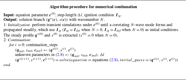
The algorithmic procedure for solving (2.8) is presented in table 2. In the procedure, the function $solve$ applies the Newton–Raphson iteration method.

Table 2.

Algorithmic procedure for numerical continuation.

Transient simulations of the combustion modes and numerical continuation were performed using a self-developed code, the codes are available at https://github.com/luofx23/RDC-Cont.

2.2.3. Formulation of MC

The numerical continuation method was used to calculate a continuous branch of solutions with varying equation parameters $\boldsymbol{c}$ starting at profiles $(\boldsymbol{q}^{*(0)} (\boldsymbol{c}^{(0)}), s^{(0)} (\boldsymbol{c}^{(0)}))$ obtained from the transient simulation results. In addition, because the Newton–Raphson iteration tends to converge to the solutions closest to the initial guess, the solutions on the branch will have the same wavenumber $N$ as $\boldsymbol{q}^{*(0)}$ .

However, within the scope of this method, when it comes to solving for $(\boldsymbol{q}^*(\boldsymbol{c}), s(\boldsymbol{c}))$ with wavenumbers $N$ , one has to provide transient simulation results with the same $N$ to start the continuation. This becomes a problem because a steadily evolved mode can only be obtained by transient simulations when it is stable. Thus, a trial-and-error process is required to search through the entire equation parameter space and identify the appropriate parameters that can produce the stable modes with corresponding wavenumbers. Another limitation of this method is that for some $N$ , the modes may be unstable across the entire equation parameter space, or even without such a solution for (2.5) and (2.6), which make these modes impossible to be obtained through transient simulations. Therefore, the range of $N$ ( $[N_{{min}}, N_{{max}}]$ ) under $\boldsymbol{c}$ cannot be determined, which compromises the completeness of the multiplicity of solutions to (2.5) and (2.6). Moreover, a quantitative LSA cannot be conducted without the unperturbed solution of a particular mode as the base state (Åkervik et al. Reference Åkervik, Brandt, Henningson, Hœpffner, Marxen and Schlatter2006; Shaabani-Ardali, Sipp & Lesshafft Reference Shaabani-Ardali, Sipp and Lesshafft2017). Nevertheless, by formulating MC in this study, the complete existence of the corotating $N$ -wave modes, that is, the range of existed $N$ under a certain set of equation parameters $\boldsymbol{c}$ , can be quantitatively computed.

Note that when $N$ = 0, the situation is not as complex. In this case, the mode solution for $N$ = 0 corresponds to the solution of (2.5) without terms of spatial gradients and wave speed $s$ . The solution of this form of the equations is exclusively the deflagration mode, allowing us to obtain the solution branch for $N$ = 0 by using procedures provided in table 2. Therefore, in the subsequent discussion of this section, we focus only on cases where $N \gt 0$ . Before introducing the MC, the self-similarity of the profile of the $N$ -wave mode was illustrated. For a baseline combustor circumference $L_{{base}}$ , the following relation holds within the domains $[0, L_{{base}}/n]$ :

(2.9) \begin{equation} \begin{array}{c} \left (\boldsymbol{q}^{*}\left (X ; \boldsymbol{c}, L_{{base }}\right ), s\left (\boldsymbol{c}, L_{{base }}\right )\right )_{N=n}=\left (\boldsymbol{q}^{*}\left (X ; \boldsymbol{c}, L_{{base }} / n\right ), s\left (\boldsymbol{c}, L_{{base }} / n\right )\right )_{N=1}, \\[6pt] X \in \left [0, L_{{base }} / n\right ], n=1,2,3, \ldots \end{array} \end{equation}

where the subscript $(\boldsymbol{q}^*, s)_{N = n}$ indicates that $\boldsymbol{q}^*$ represents the profile of the $n$ -wave mode. This property is shown in figure 4.

Figure 4.

Pressure profiles obtained from (2.5) and (2.6) with $Da$ = 128.7, $\beta$ = 0.08, $A^+$ = 0.2, $A^-$ = 1.0, $L_{{base}}$ = 24. Two pressure profiles are solved under different combustor circumference $L$ . The solid line is solved under $L = L_{{base}}$ , and the dashed line is solved under $L = L_{{base}}/2$ .

In figure 4, two pressure profiles obtained by solving (2.5) and (2.6) under the parameter set $\boldsymbol{c} = [Da = 128.7, \beta = 0.08, A^+ = 0.2, A^- = 1.0]$ are shown, where the solid line is $\boldsymbol{q}^*(X; \boldsymbol{c}, L_{{base}})_{N = 2}, L_{{base}} = 24$ , and the dashed line is $\boldsymbol{q}^*(X; \boldsymbol{c}, L_{{base}}/2)_{N = 1}$ . The two profiles coincide within the range $[0, L_{{base}}/2]$ , implying that the two-wave mode profile can be reconstructed from the presented one-wave mode by repeating the profile twice in the domain, as presented by the reconstruction equations as follows with $n$ = 2:

(2.10) \begin{align} & \boldsymbol{q}^{*}\left (X ; \boldsymbol{c}, L_{{base }}\right )_{N=n} \nonumber\\[6pt]& =\left \{\begin{array}{l} \boldsymbol{q}^{*}\left (X ; \boldsymbol{c}, L_{{base }} / n\right )_{N=1}, X \in \left [0, L_{{base }} / n\right ] \nonumber\\[6pt] \boldsymbol{q}^{*}\left (X-L_{{base }} / n ; \boldsymbol{c}, L_{{base }} / n\right )_{N=1}, X \in \left (L_{{base }} / n, 2 L_{{base }} / n\right ] \nonumber\\[6pt] \cdots \\[6pt] \boldsymbol{q}^{*}\left (X-(n-1) L_{{base }} / n ; \boldsymbol{c}, L_{{base }} / n\right )_{N=1}, X \in \left ((n-1) L_{{base }} / n, L_{{base }}\right ]. \end{array}\right .\\ \end{align}

This property of self-similarity allows us to use a one-wave mode at a combustor with different circumferences ( $L = L_{{base}}/N$ ) to represent any $N$ -wave mode at the combustor with a baseline circumference $L_{{base}}$ .

To solve the one-wave mode under different circumferences $L$ , spatial scaling is performed on (2.8), and $\boldsymbol{c}$ is replaced by $L$ in equations of $\boldsymbol{\tau }_{\textit{init}}$ :

(2.11) \begin{equation} \begin{array}{c} X=L \tilde {x}, \\[6pt] s\left (\boldsymbol{q}^{*}\right )_{\tilde {x}}+\boldsymbol{f}\left (\boldsymbol{q}^{*}\right )_{\tilde {x}}+L\left (\boldsymbol{S}_{{inj }}\left (\boldsymbol{q}^{*} ; \boldsymbol{c}\right )-\boldsymbol{S}_{{ex}}\left (\boldsymbol{q}^{*} ; \boldsymbol{c}\right )+\boldsymbol{S}\left (\boldsymbol{q}^{*} ; \boldsymbol{c}\right )\right )=\mathbf{0}, \\[12pt]\boldsymbol{q}^{*}(\tilde {x}=0)=\boldsymbol{q}^{*}(\tilde {x}=1), \\[12pt]\int _{0}^{1} \boldsymbol{q}^{*}(\tilde {x}) \dfrac {\textrm{d}}{\textrm{ d} \tilde {x}} \boldsymbol{q}_{{init }}(\tilde {x}) \textrm{d} \tilde {x}=0, \\[12pt] \boldsymbol{\tau }_{{init }}\left (\boldsymbol{q}^{*}-\boldsymbol{q}_{{init }}, s-s_{{init }}, L-L_{{init }}\right )^{\textrm{T}}=\Delta l, \\[12pt] \left ({\unicode{x1D63F}}_{\boldsymbol{q}_{{init }}, s_{{init }}, L_{{init }}} \boldsymbol{H}\right ) \boldsymbol{\tau }_{{init }}^{T}=0 . \end{array} \end{equation}

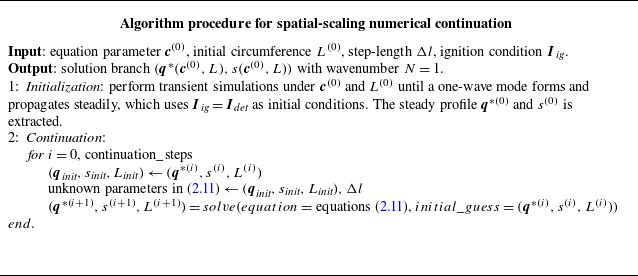
Thus, variable $L$ in the boundary conditions is explicitly incorporated into the equations. In (2.11), $\boldsymbol{c}$ is set as a set of given parameters $\boldsymbol{c}^{(0)}$ . The pseudoarclength continuation presented in table 2 can be adapted here to solve (2.11) with a few modifications, as presented in table 3. In this process, we obtain the solution branch $(\boldsymbol{q}^*(\boldsymbol{c}^{(0)}, L), s (\boldsymbol{c}^{(0)}, L))$ .

Table 3.

Algorithmic procedure for spatial-scaling numerical continuation.

At the beginning of § 2, in the introduction to the method flow, we select $L^{(0)}$ as $L_{{base}}$ . However, $L^{(0)}$ can be chosen as any other circumference, as long as a stable single-wave mode can be obtained through transient simulation at that $L^{(0)}$ .

From solution branch $(\boldsymbol{q}^*(\boldsymbol{c}^{(0)}, L), s (\boldsymbol{c}^{(0)}, L))$ , an inverse function of $s = s (\boldsymbol{c}^{(0)}, L)$ can be defined by (2.12), which is MC,

(2.12) \begin{equation} \frac {L}{L_{{base }}}=g\big (s ; \boldsymbol{c}^{(0)}\big ), \end{equation}

on the MC, points with a value of 1 / $N$ correspond to $L$ = $L_{\textit{base}}$ / $N$ , representing the $N$ -wave mode. For the above calculation, it is crucial to determine the range of $L$ (that is, the boundaries of the maximum and minimum values of MC). Physically, $L$ cannot be zero or infinitely large, and the physical constraints on $L$ also limit the possible range of $N$ . In § 4, we will discuss these physical constraints in detail, which define the maximum and minimum boundaries of MC. Through the ranges the MC, one can obtain the existence boundaries for $N$ -wave modes under parameter $\boldsymbol{c}_0$ with combustor circumference $L_{{base}}$ , that is, $N_{{min}}$ and $N_{{max}}$ .

After determining the boundary of $N$ , we can select the solution $(\boldsymbol{q}^*(\boldsymbol{c}^{(0)}, L), s (\boldsymbol{c}^{(0)}, L))$ from the spatial-scaling continuation that satisfies $L$ = $L_{{base}}$ / $N$ . Using the reconstruction equations (2.10), the profiles and wave speeds of all $N$ -wave modes under the baseline perimeter $L_{{base}}$ can be obtained.

2.3. Linear stability analysis of combustion modes in RDC

The stability of mode $\boldsymbol{q}^*$ , which means that whether initial perturbation of the mode $\boldsymbol{q}^*$ will increase (identified as unstable) or decrease (identified as stable) as time grows, has a significant impact on the dynamic behaviour of the combustion modes. The LSA of mode $\boldsymbol{q}^*$ is performed in this section. Considering $\boldsymbol{q}^*$ as the base state, expand (2.4) with small disturbances and neglect the higher-order terms, yielding

(2.13) \begin{align}&\qquad\qquad\qquad\quad \boldsymbol{q}^{\prime } =\boldsymbol{q}-\boldsymbol{q}^{*},\left \|\boldsymbol{q}^{\prime }\right \|=O(\varepsilon ), \varepsilon \ll 1, \end{align}

(2.14) \begin{align} \boldsymbol{q}_{t}^{\prime } &=-\left ({\unicode{x1D63F}} \boldsymbol{f}_{\boldsymbol{q}^{*}} \boldsymbol{q}^{\prime }-s \boldsymbol{q}^{\prime }\right )_{X}+\big ({\unicode{x1D63F}} \boldsymbol{S}_{{inj}\boldsymbol{q}^{*}}-{\unicode{x1D63F}} \boldsymbol{S}_{{ex}_{\boldsymbol{q}^{*}}}+{\unicode{x1D63F}} \boldsymbol{S}_{\boldsymbol{q}^{*}}\big ) \boldsymbol{q}^{\prime }=\mathcal{L}_{\boldsymbol{q}^{*}} \boldsymbol{q}^{\prime }, \end{align}

where ${\unicode{x1D63F}}\boldsymbol{X}_{\boldsymbol{q}^*}$ represents the Jacobian matrix of function $\boldsymbol{X}$ (where $\boldsymbol{X} = \boldsymbol{f}, \boldsymbol{S}_{\textit{inj}}, \boldsymbol{S}_{{ex}}, \boldsymbol{S}$ ) with respect to the state variable $\boldsymbol{q}^*$ , and $\mathcal{L}_{\boldsymbol{q}^*}$ denotes the linear operator of (2.4) under the base state $\boldsymbol{q}^*$ . For the linear eigenvalue system described as

(2.15) \begin{equation} \begin{array}{c} \mathcal{L}_{\boldsymbol{q}^{*}} \boldsymbol{q}_{\textit{eig }}^{\prime }=\zeta \boldsymbol{q}_{\textit{eig }}^{\prime }, \boldsymbol{q}_{\textit{eig }}^{\prime } \in \mathbb{C}^{2 m}, \\[12pt] \boldsymbol{q}_{\textit{eig }}^{\prime }(0, t)=\boldsymbol{q}_{\textit{eig }}^{\prime }(L, t) e^{i \sigma }, \sigma \in [0,2 \pi ], \end{array} \end{equation}

where $\zeta$ represents the eigenvalue of $\mathcal{L}_{\boldsymbol{q}^*}$ , which characterizes the growth rate of perturbations over time, $m$ is the dimension of $\boldsymbol{q}^{*}$ and $e^{\textrm{i}\sigma }$ represents the Floquet multiplier, which characterizes the growth rate of perturbations over space; $\boldsymbol{q}^\prime _{{eig}}$ denotes the eigenmode of $\mathcal{L}_{\boldsymbol{q}^*}$ . The boundary condition in (2.15) is a direct result from spatial Floquet analysis. Detailed derivations of this condition can be found in Sandstede (Reference Sandstede2002), Rademacher et al. (Reference Rademacher, Sandstede and Scheel2007) and Sherratt (Reference Sherratt2012). Owing to the translation symmetry induced by periodic boundary conditions, when $\sigma$ = 0, $\mathcal{L}_{\boldsymbol{q}^*}$ always has a zero eigenvalue, corresponding to the eigenmode $(\boldsymbol{q}^*)_X$ ,

(2.16) \begin{equation} \mathcal{L}_{\boldsymbol{q}^{*}}(\boldsymbol{q}^{*})_{X}=\mathbf{0} . \end{equation}

This set of special eigenvalues and eigenmodes is caused by translation symmetry and does not contribute to the physical properties of (2.4) (Sandstede Reference Sandstede2002). Therefore, unless otherwise specified, the eigenvalues and eigenmodes considered in this study do not include this specific set of the eigenvalue and eigenmode. After deriving the linearized equations (2.14) for RDC, the eigenmode corresponding to the largest real part of the eigenvalue in (2.15) is defined as the most unstable mode. When (2.14) satisfies

(2.17) \begin{equation} \lim _{t \rightarrow \infty }\left \|\boldsymbol{q}^{\prime }\right \|=0, \forall \boldsymbol{q}^{\prime }(X, t=0), \end{equation}

initial perturbation gradually decreases, therefore $\boldsymbol{q}^*$ is identified as a stable mode. In this case, (2.15) require

(2.18) \begin{equation} \Big (\max _{\zeta } {Re}(\zeta )\Big )\lt 0 . \end{equation}

When the real part of the eigenvalue corresponding to the most unstable mode is greater than zero, initial perturbation will grow exponentially, therefore $\boldsymbol{q}^*$ is identified as an unstable mode. In this work, the evolution of growing initial perturbation is called `unstable evolution’. Note that when the base state $\boldsymbol{q}^*$ is a deflagration mode, if (2.18) does not hold, that is, when $\boldsymbol{q}^*$ is an unstable deflagration mode, the perturbations of $\boldsymbol{q}^*$ are likely to induce oscillatory evolution of $\boldsymbol{q}^*$ , which may lead to an acoustic mode.

In this study, we focused on the physical interpretation of the most unstable eigenmodes and their eigenvalues. These eigenmodes depict unstable flow structures that undergo exponential growth once a disturbance is applied, and the growth rates and frequencies of these structures are determined by their eigenvalues. Therefore, the dominant unstable structures in the flow field and their evolution can be quantitatively reproduced by the temporal integration of the unstable eigenmodes, which implies solving the initial value problem of (2.14),

(2.19) \begin{equation} \begin{array}{c} \boldsymbol{q}_{t}^{\prime }=-\left ({\unicode{x1D63F}} \boldsymbol{f}_{\boldsymbol{\! q}^{*}} \boldsymbol{q}^{\prime }-s \boldsymbol{q}^{\prime }\right )_{X}+\left ({\unicode{x1D63F}} \boldsymbol{S}_{{inj} \boldsymbol{q}^{*}}-{\unicode{x1D63F}} \boldsymbol{S}_{{ex} \boldsymbol{q}^{*}}+{\unicode{x1D63F}} \boldsymbol{S}_{\boldsymbol{q}^{*}}\right ) \boldsymbol{q}^{\prime }=\mathcal{L}_{\boldsymbol{q}^{*}} \boldsymbol{q}^{\prime }, \\[6pt] \boldsymbol{q}^{\prime }(X, t=0)=\boldsymbol{q}_{\textit{eig }}^{\prime }. \end{array} \end{equation}

In this study, (2.19) is simulated using the same time-stepping scheme as in § 2.2.1.

3.1. Steady behaviour of combustion modes

This section focuses on demonstrating the steady-state behaviour of the RDC system (with circumference $L_{{base}}$ ), that is, the existence of mode $\boldsymbol{q}^*$ . Under the configurations shown in figure 5(a), the RDC system simultaneously exhibits five different modes $\boldsymbol{q}^*(X/L_{{base}}; \boldsymbol{c}, L_{{base}})$ under a given set of $\boldsymbol{c}$ , each representing the presence of $N$ = 0, 1, 2, 3 and 4 ( $N$ = 0 represents deflagration) waves with the same speed and direction travelling in the combustor. Figure 5(a) presents the profiles of these modes and the corresponding wave speeds $s$ . Figure 5(a) also presents a family of pressure profiles $p(X; \boldsymbol{c}, L)$ of one-wave mode and their corresponding wave speeds $s(L)$ , where the $X$ -axis represents the spatial coordinate of the combustor (in the travelling wave coordinate). These profiles were obtained using the numerical continuation schemes introduced in § 2.2.3. As shown in figure 5(a), the wave speeds and profiles of the one-wave modes fully coincide with the corotating $N$ -wave profile at $L$ = $L_{{base}}$ within a single spatial period.

In figure 5(a), the envelope line of the cutoff points $(X / L_{{base}} = L / L_{{base}})$ for each profile is highlighted. The range of this curve contains the necessary information about the existence of $\boldsymbol{q}^*$ under a fixed set of parameters $\boldsymbol{c}$ , which is essentially the MC defined in (2.12). Section 4.1 provided a detailed interpretation of MC. Sections 4.2 and 4.3 investigate the required physical constraints to derive the boundaries of the MC. The upper and lower boundaries of the MC change with the varying equation parameter $\boldsymbol{c}$ , determining different types of existing modes under different equation parameters. Figure 5(b) presents the relationship between the MCs and one of the equation parameters $c$ by changing the $p$ axis in figure 5(a) into parameter axis $c$ , where the upper and lower boundaries of the MCs are marked on both ends of the MCs. Section 4.4 highlights the influence of changes in the equation parameters on the boundaries of the MCs.

3.2. Dynamic behaviour of combustion modes

In this section, the typical dynamic behaviour of the RDC system modes is demonstrated in conjunction with the stability of $\boldsymbol{q}^*$ . A complete outline of the studied dynamics is shown in figure 5(b). For an MC under a specific equation parameter $c_i$ , the marked dots on the curve represent the existing modes, where a solid dot represents a stable mode and a hollow dot represents an unstable mode. By projecting the MCs with varying equation parameters onto the $c{-}s$ plane and preserving only the points representing $N$ -wave modes in the baseline combustor, the branches of all $N$ -wave modes with a fixed circumference of the combustor $L_{{base}}$ can be obtained as shown on the right-hand side of figure 5(b). The dashed and solid parts of the branches are used to distinguish between the unstable and stable branches. The stability attributes of each mode are determined by LSA introduced in § 2.3. On each branch, the intersection points of the stable and unstable branches are marked as bifurcation points. On either side of the bifurcation point, the stability of the mode branches undergoes a transition. Depending on the manner of the transition, there are two types of bifurcation in (2.1): saddle-node and Hopf bifurcations. When two fixed points of a nonlinear dynamical system collide locally and disappear as the parameter passes through the bifurcation point, this type of bifurcation is referred to as a saddle-node bifurcation, as indicated by the triangular symbols in figure 5(b). However, when the eigenvalues of the dynamic system with the largest real part form a pair of complex conjugate eigenvalues, and the original fixed point becomes unstable after passing through the bifurcation point, the system exhibits oscillatory behaviour known as a Hopf bifurcation (Strogatz Reference Strogatz2024). This type of bifurcation is represented by diamond symbols in figure 5(b). A further exploration of the features of the mode branches is presented in § 5.1.

Dominated by the stability attributes of the branches, the combustion modes in (2.1) exhibit complex dynamic behaviours. To better explain these behaviours, we use denomination $(N = n, c)_{\textit{stable}}$ , which means a stable $n$ -wave mode under equation parameter $c$ , to refer to the points in figure 5(b). Processes A1 (cold flow $\rightarrow (N = 1, c_1)_{\textit{stable}}$ ) and A2 (cold flow $\rightarrow (N = 2, c_1)_{\textit{stable}}$ ) in figure 5(b) indicate that under varied ignition conditions, the combustor could converge to distinct combustion modes from cold flow via a mode formation process. This dynamic behaviour is investigated in § 5.2. Furthermore, the response to perturbations in combustion modes is also the focus of this study. By imposing a perturbation on equation parameter $c$ which lead the combustor across a bifurcation point, instabilities and mode transition process B1 ( $(N = 1, c_1)_{\textit{stable}} \rightarrow (N = 3, c_2)_{\textit{stable}}$ ), which crosses a saddle-node bifurcation point, or B2 ( $(N = 2, c_1)_{\textit{stable}} \rightarrow (N = 2, c_2)_{\textit{stable}} \rightarrow (N = 3, c_2)_{\textit{stable}}$ ) would occur, which is investigated in § 5.3. On the other hand, by imposing disturbances on the state variables of the combustor under fixed equation parameters, instabilities and mode transition process C1 ( $(N = 4, c_1)_{\textit{stable}} \rightarrow (N = 1, c_1)_{\textit{stable}}$ ) or C2 ( $(N = 4, c_1)_{\textit{stable}} \rightarrow (N = 2, c_1)_{\textit{stable}}$ ) would also occur, depending on the symmetries of the disturbances, which is investigated in § 5.4. The LSA was employed to quantitatively analyse the dynamic interactions underlying these processes.

4.1. Complete existence of corotating N-wave modes

With the baseline equation parameters $\boldsymbol{c}_{{base}} = [Da = 128.7, \beta = 0.09, A^+ = 0.2, A^- = 1.0]$ and baseline circumference ( $L_{{base}}$ = 24), (2.11) are solved by methods mentioned in § 2.2.3 to obtain a family of one-wave mode with different $L$ ; the results are shown in figure 6. Figure 6(a) shows the pressure profiles $p(X; \boldsymbol{c}_{{base}}, L)$ corresponding to different combustor circumferences $L$ . Projecting figure 6(a) onto the $s{-}X$ plane yields figure 6(b). By extracting the endpoints of each profile, the MC $g(s; \boldsymbol{c}_{{base}})$ was obtained, as highlighted in figure 6(c). Points with a value of 1/ $N$ are marked, to represent the $N$ -wave modes.

Figure 6.

(a) Family of pressure profiles $p(X;L)$ for single-wave modes at different combustor circumferences $L$ while equation parameters $\boldsymbol{c}$ are fixed as baseline values. (b) Projection of figure 6(a) onto the $s{-}X$ plane. The envelope formed by the end points of $p(X; L)$ is high-lighted. Circles denote points corresponding to $L / L_{{base}} = 1 / N$ ( $N = 1, 2, 3, 4$ ). (c) The envelope curve in figure 6(b), i.e. the MC.

The existence of modes $\boldsymbol{q}^*$ is determined by the range of MC ( $g$ ). The $g_{{min}}$ determines the $N_{{max}}$ , and the $g_{{max}}$ determines the $N_{{min}}$ . Mathematically, the MC can be extended along both ends through numerical continuation, but physical constraints must be imposed to ensure that the propagation of detonation waves conforms to actual aerodynamic processes. The structure of the detonation wave is characterized by a precursor shock wave followed by a reaction induction zone and an exothermic zone. Owing to the existence of the precursor shock wave, the Mach number of the incoming flow relative to the wavefront must be greater than one, and according to the Prandtl relation satisfied by shock waves, the relative Mach number behind the precursor shock wave must be less than one. These two physical constraints prevent the wave speed $s$ in the MC from indefinitely extending at both ends.

To investigate how these two physical constraints limit the range of $g$ , it is necessary to examine the relative Mach numbers of the detonation waves, $Ma_{\textit{r}0}$ and $Ma_{\textit{r}1}$ , corresponding to each point on $g$ . Figure 7 shows the preshock and postshock positions based on the pressure and relative Mach number profiles of the one-wave mode under the baseline equation parameters and baseline combustor circumference. Here, the relative Mach number is defined as

(4.1) \begin{equation} M a_{\textit{r}}=\frac {u-s}{\sqrt {\gamma R T}}, \end{equation}

where $s$ represents the wave speed corresponding to the mode. Based on the grid size, the wavefront point and the wave rear point are defined as the first grid points before and after the precursor shock wave discontinuity, where the relative Mach number reaches the maximum and minimum values across the entire domain, respectively.

Figure 7.

The pressure profile and the relative Mach number profile of the one-wave mode when the combustor length is $L_{{base}}$ and the equation parameters are at their baseline values.

4.2. The MC lower boundary: the preshock Mach number

Figure 8(a) displays the partial MC from figure 6(c) along with their corresponding preshock Mach numbers ( $Ma_{\textit{r}0}$ ). When the absolute value of the wave speed decreased to a certain extent, $Ma_{\textit{r}0}$ reached the sonic point. At this point, the intensity of the shock wave became zero, representing the degeneration of the flow field into the deflagration mode with a spatially uniform state, as shown in figure 8(b,c). This critical point, where $Ma_{\textit{r}0}$ = 1, is referred to as the sonic point in this study, determining the lower boundary of the MC. In figure 8(a), this boundary is slightly below 0.2 (1/5) but greater than 1/6, indicating that under $\boldsymbol{c}_{{base}}$ and $L_{{base}}$ , the RDC system can accommodate at most a five-wave mode.

Figure 8.

(a) The MC and its corresponding preshock and postshock Mach number when $Da = 128.7, \beta = 0.09, A^+ = 0.2, A^- = 1.0$ and $L_{{base}} = 24$ . (b) Pressure profile for $Ma_{\textrm{r0}} = 1$ . (c) Profile of relative Mach numbers when $Ma_{\textrm{r0}} = 1$ .

4.3. The MC upper boundary: baseline circumference and postshock Mach number

Because $L_{{base}}$ is fixed, for the $N$ -wave modes, their corresponding minimum spatial periods must be less than or equal to $L_{{base}}$ , which requires that the value of MC not exceed one. However, whether MC is allowed to take the value one depends on whether $Ma_{\textit{r}1}\lt 1$ can be ensured at that point. Therefore, the upper boundary of the MC was the result of the joint constraint of the baseline circumference of the combustor and the postshock Mach number,

(4.2) \begin{equation} \begin{array}{l} \left (\frac {L}{L_{{base }}}\right )^*=\arg \left (M a_{\textit{r} 1}\left (\frac {L}{L_{{base }}}\right )=1\right ), \\[12pt] \left (\frac {L}{L_{{base }}}\right )_{max }=\min \left (1,\left (\frac {L}{L_{{base }}}\right )^*\right ) . \end{array} \end{equation}

Under the operating conditions shown in figure 6(c), $(L/L_{{base}})^*\gt 1$ , the upper boundary of MC equals one, indicating that for an RDC system with $L = L_{{base}}$ under the baseline equation parameters, a one-wave mode is guaranteed to exist.

However, when changing the equation parameters, the situation may arise where $(L/L_{{base}})^*\lt 1$ . Figure 9(a) illustrates a portion near the upper boundary of MC and its corresponding profile of $Ma_{\textit{r}1}$ when the equation parameter is set to $\beta$ = 0.105 (with other parameters remaining at baseline values).

Figure 9.

(a) The MC and its corresponding $Ma_{\textrm{r1}}$ when $Da = 128.7, \beta = 0.105, A^+ = 0.2, A^- = 1.0$ and $L_{{base}} = 24$ .The non-detonation branch is represented by dashed lines. (b) The pressure profile corresponding to the points on MC with wave speeds of −2.90 and −3.08. The non-detonation mode is indicated by dashed lines. (c) Relative Mach-number profiles.

Note that when $Ma_{\textit{r}1}$ = 1, the MC value was approximately 0.8, which is still less than one. Under this set of operating conditions, when the absolute value of the wave speed increases to a certain extent, $Ma_{\textit{r}1}$ reaches the sonic point, that is, $L/L_{{base}}=(L/L_{{base}})^*$ . At this point, the shock waves no longer exist in the flow field, and the obtained mode is no longer a detonation mode which requires the existence of a precursor shock wave. The branch that consists of these specific modes is indicated by the dashed line and is termed a non-detonation branch, which needs to be discarded for the purpose of this study. Point $(s^*,(L/L_{{base}})^*)$ is defined as the ‘turning point’, a point where the slope of the MC varies significantly on both sides. Figures 9(b) and 9(c) select the pressure profile (figure 9 b) and the profile of relative Mach number (figure 9 c) at wave speeds of $s$ = −2.90 (detonation mode with the existence of a precursor shock wave, depicted by solid line) and $s$ = −3.08 (non-detonation mode without the existence of the precursor shock wave, depicted by dashed line), from which the disappearance of the precursor shock wave after the increment of the absolute value of wave speed can be clearly observed. Thus, the turning point determined the upper boundary of the MC, approximately 0.8. This suggests that, for an RDC system with $L_{{base}}$ , a one-wave mode cannot be formed under this set of equation parameters.

4.4. Influence of equation parameters on the extrema of the MC

Once the lower and upper boundaries of the MC have been identified, this section investigates the influence of equation parameter $\boldsymbol{c}$ on these boundaries. Here, four different families of MCs are obtained by separately varying $Da$ , $\beta$ , $A^+$ and $A^-$ . When one parameter is changed, the other equation parameters remain at their baseline values, and the baseline circumference of the combustor remains unchanged. The results for the four families of MCs are shown in figure 10.

Figure 10.

Families of MCs with varying equation parameters. The boundaries formed by the envelope of turning points and sonic points are marked. Non-detonation branches are represented by dashed lines: (a) MCs varying only $Da$ ; (b) MCs varying only $\beta$ ; (c) MCs varying only $A^+$ ; (d) MCs varying only $A^-$ .

The variation in the lower boundaries of MCs, that is, the sonic point boundary, is investigated firstly. In figure 10(a), the increase in $Da$ signifies an enhancement in the speed of the chemical reaction compared with the convective velocity. This allowed more time for heat to accumulate in the combustor, leading to an increase in the temperature of the combustible mixture ahead of the detonation wave. Consequently, at the same wave speed, the preshock Mach number decreased, bringing the mode closer to the sonic boundary. Hence, the sonic point boundary of the MC exhibits a decreasing trend with increasing $Da$ . In figure 10(b), an increase in $\beta$ results in faster completion of the mixing of the propellant injected into the combustor, leading to a higher concentration of propellant in the filling region. This enhanced the heat release rate of the chemical reaction, thereby promoting an increase in the temperature of the combustible mixture ahead of the detonation wave. In figure 10(c), the increase in $A^+$ prolongs the time required for the recovery and reconstruction of the postwave propellant injection, because a larger injection area exerts a greater influence on the injection process in the high-pressure region behind the detonation wave. This weakened the energy injection process of the system, thereby reducing the average temperature ahead of the detonation wave at the same wave speed and increasing an increase in the preshock Mach number. Consequently, the sonic line showed an increasing trend. In figure 10(d), the increase in $A^-$ expands the exit area for combustion product, which enhances the energy ejection process of the system and reduces the average temperature ahead of the detonation wave as well. This caused the sonic line in figure 10(d) to share the same increasing trend as that shown in figure 10(c).

Overall, increases in $Da$ and $\beta$ promoted the input and accumulation of energy in the system, enhancing the net rate of energy gain. This results in a decrease in the minimum value of the MCs, favouring the generation of multiwave modes. However, an increase in $A^+$ introduces a higher propellant flow rate, but its benefits cannot offset the negative effect of hindering the reconstruction of the propellant injection. This inhibits the input of energy into the system, leading to an increase in the minimum value of the characteristic curves, thereby promoting the degeneration of multiwave modes. The increase in $A^-$ plays a similar role as $A^+$ by increasing the output of energy in the system.

The upper boundaries of the MCs were determined based on the position of the turning point, and the envelope formed by the turning points constituted the turning-point boundary. In figures 10(a) and 10(b), turning points are observed in MCs with values less than one, occurring at higher values of $Da$ , $\beta$ and $A^-$ . The points above the turning points represent non-detonation modes where the precursor shock wave disappears, denoted by dashed lines in this special region. This indicates that the lower-wavenumber modes allowed by the system are more likely to disappear with increasing net speed of the energy input. The variation in the maximum and minimum values of the MCs shows that the number of $N$ -wave modes in the system tends to increase with the increase in net energy input. This indicates that the higher-wavenumber modes in the combustor have a higher energy carrying capacity than the lower-wavenumber modes.

The analysis in this section quantitatively delineates the number and types of $N$ -wave modes existing in the RDC, answering what types of $N$ -wave mode RDC systems exist under a fixed set of equation parameters $\boldsymbol{c}$ . The minimum wavenumber allowed by RDC is determined by whether the postshock Mach number crosses the sonic point, which reflects the blocking effect of detonation waves: under the same set of equation parameters, lower-wavenumber modes have higher wave speeds than higher-wavenumber modes. Lower-wavenumber modes have greater mass and energy fluxes than higher-wavenumber modes; when the postwave reaches the ‘blocked’ state, the precursor shock wave cannot consume more flow, thus restricting the maximum wave speed of RDC modes, which also corresponds to the limit of minimum wavenumber of the modes.

However, the maximum wavenumber allowed by the RDC is determined by whether the preshock Mach number crosses the sonic point, which marks the limit of the maximum energy capacity of the detonation waves. If the system accumulates increasing input energy, its average temperature will be elevated and the proportion of deflagration combustion will share the same increasing trend. The deflagration that coexists with detonation is called secondary combustion. Secondary combustion is a diffusion combustion that enhances the energy of the preshock combustible mixture and reduces the preshock Mach number, weakening the detonation intensity and promoting the degeneration of detonation modes into deflagration modes. This secondary combustion effect on detonation modes has been observed and validated by numerous numerical simulations and experiments (Wang & Wang Reference Wang and Wang2016; Chacon & Gamba Reference Chacon and Gamba2019; Feleo, Chacon & Gamba Reference Feleo, Chacon and Gamba2019; Prakash et al. Reference Prakash, Fiévet, Raman, Burr and Yu2020; Sato et al. Reference Sato, Chacon, White, Raman and Gamba2021; Raman, Prakash & Gamba Reference Raman, Prakash and Gamba2023). The restriction of MCs by the preshock and postshock Mach numbers fundamentally reflects the constraints imposed by the blocking effect and secondary combustion on the types and wavenumbers of the corotating $N$ -wave modes.

5.1. Branch feature overview

In this section, $Da$ , $\beta$ , $A^+$ and $A^-$ are selected as bifurcation parameters. The profiles and wave speeds $(\boldsymbol{q}^*(X; \boldsymbol{c}_{{base}}, L_{{base}}/N),s(\boldsymbol{c}_{{base}}, L_{{base}}/N))_{N=1}$ calculated in figure 6(a) with $N$ = 1, 2, 3 and 4 were collected and applied to reconstruction equation (2.10) to obtain the profiles and wave speeds of $(\boldsymbol{q}^*(X; \boldsymbol{c}_{{base}}, L_{{base}}),s(\boldsymbol{c}_{{base}}, L_{{base}}))_{N=n}$ , $n$ = 1,2,3,4. The $N$ = 0 mode under $\boldsymbol{c}_{{base}}$ is obtained by methods mentioned in table 2. These $N$ -wave solutions ( $N$ = 0, 1, 2, 3, 4) are chosen as starting points for numerical continuation using (2.8), resulting in complete branches of $N$ -wave mode and their corresponding wave speeds $(\boldsymbol{q}^*(\textit {c}), s(\textit {c})) (c = Da, \beta , A^+, A^-)$ . When varying one bifurcation parameter, the other equation parameters remain unchanged from the baseline parameters in § 4, and the circumference $L$ of combustor is fixed at 24 throughout § 5.

The computational results are shown in figure 11. In figure 11, the mode branches are characterized by pressure peak values, with curves representing the corotating $N$ -wave modes for $N$ = 1, 2, 3 and 4, whereas the $N$ = 0 branch represents the set of deflagration modes. The solid portions in each mode branch represent the global stable modes, while the dashed portions represent global unstable modes. The types of bifurcation points in the branches are marked with triangular and diamond markers representing the saddle-node and Hopf bifurcations, respectively.

Figure 11.

Mode branches of $N$ -wave modes, the dashed portions represent global unstable modes. Triangular and diamond marker individually representing the saddle-node bifurcation and Hopf bifurcation: (a) bifurcation parameter, $Da$ ; (b) bifurcation parameter, $\beta$ ; (c) bifurcation parameter, $A^+$ ; (d) bifurcation parameter, $A^-$ .

In figure 11, the changing patterns of the existence and stability of the mode branches for each mode with respect to the equation parameters are clearly observed. When the parameter range is sufficiently broad, each detonation wave mode exists only within a finite parameter range, as shown in figures 11(a) and 11(b). The disappearance of detonation wave mode branches can be divided into two cases, corresponding to the physical constraints of MCs discussed in § 4: in figures 11(a), 11(b) and 11(d), there are cases where the detonation branches exhibit a vertical trend of change (for example, the $N$ = 1 branch around $Da$ = 150 in figure 11 a; the $N$ = 1 branch around $\beta$ = 0.10 in figure 11 b; the $N$ = 1 branch around $A^-$ = 0.92 in figure 11 d), representing the crossing of the postshock Mach number over the sonic point, leading to the disappearance of the precursor shock wave and degeneration into a non-deflagration mode. In another case, the detonation mode branches merge with the deflagration mode branches with a gentle trend, indicating the crossing of the preshock Mach number over the sonic point. This results in the degeneration of the flow into a deflagration mode.

Figure 12.

Four different scenarios of mode stability patterns under the same $A^-$ .

When the postshock Mach number surpasses the sonic point (as shown by the vertical trend in detonation branches), minor changes in the equation parameters can swiftly cause a detonation mode to transition into a deflagration mode, demonstrating the RDC combustion mode’s ‘abrupt transition’ properties. However, under the same parameters, stable modes with lower wavenumbers always have a higher $p_{{max}}$ than stable modes with higher wavenumbers, and within the entire bifurcation parameter range, the modes with the highest $p_{{max}}$ are always $N$ = 1 modes. This feature suggests that one-wave modes have higher performance gains than other modes, which has also been validated in high-fidelity numerical simulations (Sheng, Cheng & Wang Reference Sheng, Cheng and Wang2023).

In addition, the stability patterns of the modes under different conditions were classified. Taking figure 11(d) as an example, the stability patterns of the mode branches with respect to bifurcation parameter $A^-$ can be divided into four different cases, each belonging to a specific parameter range as shown in figure 12.

1. (i) Scenario I. Under this set of equation parameters, there were no $N$ -wave modes in the combustor. The stable state of the RDC consists only of the deflagration mode (stable deflagration) or the longitudinal pulsating combustion mode (unstable deflagration).

2. (ii) Scenario II. Within this parameter range, although $N$ -wave modes existed, each $N$ -wave mode was unstable. In this case, the system cannot converge to stable $N$ -wave modes but tends to evolve into limit cycle states of periodic oscillations, including the longitudinal pulsating combustion mode and the counter-rotating wave mode.

3. (iii) Scenario III. Within this parameter range, the combustor contains only one type of stable $N$ -wave mode, which causes the RDC system to exhibit a high certainty in its operating modes. Regardless of the ignition conditions, as long as the combustor converges to the $N$ -wave mode, the wavenumber $N$ of this mode is guaranteed. Moreover, since this mode is stable, after the system converges, it does not experience unstable evolution under any form of small perturbation.

4. (iv) Scenario IV. Within this parameter range, more than one stable $N$ -wave mode exists. Starting with different ignition conditions, the RDC system may converge to different combustion modes. Moreover, if the flow field is subjected to significant disturbances or excitations, these modes may undergo a transition from one stable mode to another. Based on the patterns of the mode branches described above, the next section explores the dynamic behaviour of $N$ -wave modes in the RDC.

5.2. Mode formation: dependence on ignition/initial conditions

In specific ranges of the equation parameters (such as parameter range IV in figure 12), there are multiple global stable $N$ -wave modes in the combustor. Therefore, different initial conditions may cause the combustor to converge to different stable modes.

According to the branch diagram in figure 11(b), $\beta$ was set to 0.095 (other parameters remained at baseline values) to perform studies on mode formation. Under this set of equation parameters, the equations exhibit stable one-wave mode and two-wave mode simultaneously. To induce different modes in the system, different initial conditions were set based on the spatial periodicity of the system by setting different spatial periods of $L$ and $L / 2$ . Here are the specific settings: from $t$ = 0 – 10, set $\lambda = 0.5\textrm{sin}(2\pi / L x) + 0.5$ and $\lambda = 0.5\textrm{sin}(2*2\pi / L x) + 0.5$ to prefill the reactant zone(as the profile of $\lambda$ at $t = t_{{ignition}}$ shown in figures 13 a and 13 b). Choosing a sine waveform ensures the periodicity of the prefilled area and creates an asymmetry in the directions for the propagation of the ignition kernels, allowing the energy to propagate faster in the direction of decreasing $\lambda$ after ignition. This dominant direction is shown in figures 13(a) and 13(b). The establishment for a dominant direction was to suppress the generation of the counter-rotating wave mode. From $t = 10-10.20$ , set $Da(12 \lt x \lt 15) = 2000$ and $Da(0 \lt x \lt 3, 12 \lt x \lt 15) = 2000$ to simulate instantaneous ignition (specified as the ignition zone in figures 13 a and 13 b), and after $t \gt 10.20$ , restore $Da$ for the entire field. Under both conditions, the arrangement of the ignition kernels also followed the spatial periodicity of $L$ and $L / 2$ , and the ignition intensity was the same.

Figure 13.

Mode branches of $N$ -wave modes, the dashed portions represent global unstable modes. Triangular and diamond marker individually representing the saddle-node bifurcation and Hopf bifurcation. (a,b) Spatiotemporal pressure fields under individual ignition conditions and profiles at $t = t_{{ignition}}$ (profiles for $p$ ) and $t = t_{{end}}$ (profiles for $p$ ). (c,d) Amplified positions of the modes in figure 9(a) in the diagram of mode branches. (e) Mode branches varying $\beta$ (with the remaining parameters maintained at baseline values: $Da = 128.7, A^+ = 0.2, A^- = 1.0, L = 24$ ).

Figures 13(a) and 13(b) illustrate the spatiotemporal pressure field of the RDC field induced by the respective initial conditions. After the transient evolution induced by the initial ignition process, both cases converged to a stable $N$ -wave mode in the rotating direction (also marked by arrows in figures 13 a and 13 b) and spatial period of the profile consistent with the dominant direction and the spatial period established by the ignition conditions. Figures 13(c) and 13(d) show the locally amplified versions of the mode branch diagram with varying $\beta$ shown in figure 13(e), in which the position where the formed stable pressure profiles at $t = t_{{end}}$ as in figure 13(a) exists is marked.

The scenarios presented above illustrate that the formation of combustion modes in an RDC, when multiple stable $N$ -wave modes exist under specific parameters, is closely related to the initial ignition conditions. Within the framework of this study, this correlation is summarized as the spatial periodicity and symmetry in the propagation directions of ignition kernels. Under the same parameter configuration, when stable $N$ -wave modes were permitted inside the RDC, ignition conditions with a spatial period of $L / N$ and azimuthal asymmetry were more conducive to inducing the system to converge to the corresponding $N$ -wave mode. In practical RDC set-ups, the spatial periodicity conditions of $L / N$ can be achieved by evenly distributing $N$ igniters along the circumference of the combustor.

5.3. Unstable evolution of mode: dependence on parameter perturbations

When the system parameters of an RDC cross the bifurcation points of the mode branches before and after parameter perturbations, the eigenvalues with the largest real parts of the combustion modes may cross the imaginary axis, leading to occurrence of unstable evolution. The manner in which the eigenvalues cross the imaginary axis determines the bifurcation categories of combustion modes. Within the scope of this study, there are two and only two types of bifurcations for corotating $N$ -wave modes: the saddle-node bifurcation and Hopf bifurcation.

5.3.1. Saddle-node bifurcation

The branch structure of $N$ -wave modes (figure 11) shows that each mode exists within a certain parameter range. Beyond this range, the physical constraints imposed by the preshock and postshock Mach numbers limit the existence of these modes. Here, we focus on the bifurcation behaviour between the corotating $N$ -wave and the non-detonation modes. Before and after bifurcation, a detonation mode will collide with and merge into a non-detonation mode, this type of local bifurcation fits the patterns of saddle-node bifurcation.

Figure 14(a) shows the mode branch diagram near the intersection of the one-wave and non-detonation branches. Figure 14(b) shows the magnitude of the postshock Mach number $Ma_{\textit{r}1}$ corresponding to each point on the mode branches in figure 14(a). At $\beta$ = 0.103, $Ma_{\textit{r}1}$ = 1, satisfying the ‘turning point’ characteristic of MC described in § 4.3. The turning points are indicated in figures 14(a) and 14(b). At this point, as $\beta$ continues to increase, there will be no longer a precursor shock wave present in the flow field, causing the detonation mode branch to degenerate into a non-detonation branch.

Figure 14.

(a) Amplified structure near the merging point of the one-wave branch and the non-detonation branch in figure 11(b). (b) The postshock Mach number corresponding to each point on the figure 11(a). (c) The spatiotemporal evolution of the total energy field before and after applying the $\beta$ perturbation (while keeping the other parameters at their baseline values: $Da = 128.7, A^+ = 0.2, A^- = 1.0, L = 24$ ).

If the system converges to a stable one-wave mode at $\beta = 0.100$ (as indicated by the solid dot in figure 14 a), after then the parameter changes to $\beta = 0.104$ (a change of 4 $\%$ in parameter magnitude, as indicated by the hollow dot in figure 14 a). At this point, the one-wave mode has already merged with the non-detonation mode where no precursor shock wave exists. Consequently, the RDC system no longer exhibited a one-wave mode. To verify this scenario, the wave profile of the one-wave branch at $\beta = 0.100$ is selected as the initial condition, with $\beta$ changing from 0.100 to 0.104 at $t$ = 20. The transient simulation continued until the evolution of the combustion mode stabilized, as shown in figure 14(c). In the figure, the vertical line indicates the moment when the perturbation is applied to $\beta$ . The combustor maintained the propagation of a stable one-wave mode during the time interval $t$ = 0 – 20. After the perturbation occurs, the mode experiences an unstable evolution from $t$ = 20 to $t$ = 60 and then gradually converges to a stable two-wave mode. This form of unstable and mode transition processes represents the inability of the system to maintain the original mode with a stable wave speed and profile after parameter perturbation.

5.3.2. Hopf bifurcation

In addition to the merging process between branches, there is a stability exchange process that occurs in the same branch. In all cases studied in this paper, from the perspective of LSA, the change in branch stability is due to a pair of complex conjugate eigenvalues crossing the imaginary axis, which is a typical form of Hopf bifurcation. Without loss of generality, the case with the bifurcation parameter $A^-$ is selected for analysis in this section. Figure 15(a) illustrates the bifurcation region of the $N = 1$ branch when the bifurcation parameter is $A^-$ , and indicates the process of mode transition for the selected case: first, setting $A^- = 0.95$ to encourage the system to converge to a stable one-wave mode. Once the mode stabilizes, $A^-$ is set to 0.92, at which point the original mode is no longer stable, whereas the two-wave mode is stable under the current conditions, causing the system to transition from an unstable one-wave mode to a stable two-wave mode.

Figure 15.

(a) The unstable evolution and transition after perturbing $A^-$ based on the mode branch diagram. (b) Spectrum of equations (2.15) at $\sigma$ = 0 using the one-wave mode at $A^-$ = 0.95 (with other parameters held at baseline values: $Da = 128.7, \beta = 0.09, A^+ = 0.2, L = 24$ ) as base state. (c) Spectrum of equations (2.15) at $\sigma$ = 0 using the one-wave mode at $A^-$ = 0.92 as base state. Eigenvalues with largest real parts are highlighted.

Figures 15(b) and 15(c), respectively, show the spectrum of the linearized system (2.15) (at $\sigma = 0$ ) with the one-wave mode as the base state $\boldsymbol{q}^*$ when $A^- = 0.95$ and $A^- = 0.92$ . It can be observed that before and after the change in $A^-$ , a pair of conjugate eigenvalues crosses from below the imaginary axis to above the imaginary axis, which is a typical indicator of Hopf bifurcation.

The transient evolution of the above dynamics is simulated where $A^-$ varies from 0.95 to 0.92. The results are presented in figure 16. Figure 16(a) illustrates the spatiotemporal field of the process, from which the growing perturbation of the one-wave mode, followed by the reconstruction of a different stable combustion mode can be observed. Figure 16(b) shows three typical moments in the flow field: the instant when the wavenumber of the combustor is 1, the instant when the combustion mode is undergoes a transition process, and the instant when a new stable mode with a wavenumber equals to 2 is formed. These three instants demonstrate a typical unstable evolution of the mode.

Figure 16.

(a) The spatiotemporal evolution of the total energy $E$ during the unstable evolution and transition of the one-wave mode to two-wave mode at $A^- = 0.92$ (with the remaining parameters kept at their baseline values: $Da = 128.7, \beta = 0.09, A^+ = 0.2, L = 24$ ). (b) is the profile of total energy at $t$ = 50, 120 and 140 presented on the observation plane, serving as typical representatives of distinct stages of the dynamics.

To investigate the unstable evolution of the one-wave mode, the results in figure 16 were transformed into a travelling wave coordinate with wave speed equal to $s$ (the wave speed corresponding to the $N = 1$ branch at $A^- = 0.92$ ), yielding figure 17(a). This spatiotemporal field consists of two different dynamic stages: the stage where the growth of modulation instability induces oscillations of the original detonation wave, and the stage where the mode transition takes place, resulting in a different stable combustion mode. During Stage 1 in figure 17(a), phase oscillations of the detonation waves can be observed (magnified in figure 17 b), as well as the gradual formation of deflagration waves near the detonation waves, which propagate in the positive $x$ -direction (magnified in figure 17 c). The increasing amplitude of the deflagration waves drives the combustor to the Stage 2 of the dynamics. During Stage 2, the evolution of the deflagration waves triggers a deflagration-to-detonation transition (DDT) process (marked in figure 17 a), forming two new detonation waves. The two detonation waves stabilized gradually, causing the combustion mode to eventually transition from the one-wave mode to the two-wave mode.

Figure 17.

(a) The spatiotemporal evolution of figure 16 displayed in travelling wave coordinates. (b) The spatiotemporal evolution in Stage 1 of figure 17(a), showing an amplitude oscillatory modulation of the detonation waves. (c) A magnification of figure 17(b) to show the deflagration waves. (d) The spatiotemporal evolution of the most unstable eigenmode of the one-wave mode at $A^- = 0.92$ simulated in linearized system (2.14). The profile of the unstable eigenmode is highlighted. Only the real part of the total energy component is shown. (e) A magnification of figure 17(d) to show the deflagration waves.

Unlike the case of saddle-node bifurcation, where the existence of the original mode no longer holds after parameter perturbation, there is no corresponding linear stability system based on this mode; in the case of Hopf bifurcation, after parameter variation, the mode $\boldsymbol{q}^*$ that belongs to the original mode still exists. At this point, the eigenvalues and eigenmodes of the original combustion mode play crucial roles in the two aforementioned dynamic stages. Based on the linearized eigenvalue system (2.15), the real part of the largest eigenvalue and its corresponding most unstable eigenmode $\boldsymbol{q}^\prime _{{eig}} = [\rho ^\prime _{{eig}},(\rho u )^\prime _{{eig}},E^\prime _{{eig}},(\rho \lambda )^\prime _{{eig}}]^{\textrm{T}}$ (with $\boldsymbol{q}^*$ being the one-wave mode of the RDC system at $A^- = 0.92$ with $\sigma$ set to 0) are calculated. In a Hopf bifurcation, there are two eigenvalues with the largest real parts, and their corresponding eigenmodes are complex-conjugates, implying that both eigenmodes possess the same real part. Because this study focuses on the connection between the real part of the eigenmode and combustion dynamics, only one of the two conjugate eigenmodes is displayed in the following analysis. To show the correlation between the linear dynamics of the most unstable eigenmode and the nonlinear dynamics mentioned above, (2.19) is calculated. The spatiotemporal field of the linear dynamics is shown in figure 17(d) (it only displays the real part of $E^\prime _{{eig}}$ ). Figure 17(d) reproduces the modulation instability imposed on the detonation wave, as shown in figure 17(b). The growth and advection of the deflagration waves shown in figure 17(c) can be traced by magnifying the eigenmode dynamics in figure 17(e).

The linear dynamics of the most unstable eigenmode were determined using their corresponding eigenvalues. The real part of the eigenvalue dominates the magnitude growth of the eigenmode, which manifested as an oscillatory amplitude growth process observed in figure 17(b). However, the imaginary part dominates the phase shift of the eigenmode, which manifests itself as an advection process, as shown in figure 17(c). Owing to the exponential growth of the amplitude of the eigenmode under the influence of eigenvalues with positive real parts, the amplitude of the deflagration wave increases, ultimately triggering the DDT process. The above analysis shows that the linear dynamics of the unstable eigenmode are able to quantitatively extract the dominant physics governing the nonlinear dynamics in which the unstable evolution of combustion mode occurs.

Underlying the mathematical formulation of eigenmode dynamics, the quantitative behaviour of the eigenmode can also be interpreted from a physical perspective. In this case which reducing $A^-$ triggers an unstable evolution of the combustion mode, the decrease in the area $A^-$ of expansion throat restricts the exhaustion of energy behind the detonation wave, resulting in a slower temperature decrease rate in the postdetonation field. When a new round of propellant injection occurred, the propellant had a higher initial temperature, thereby promoting the formation of deflagration waves. The coexistence of the detonation and deflagration waves leads to collisions. During the collision process, the flow field ahead of the detonation wave was influenced by the deflagration waves. Deflagration waves lead to a decrease in the reactant concentration, and an increase in the temperature and pressure in the flow field ahead of the detonation wave, reducing the heat released by chemical reactions at the detonation wavefront and resulting in a decrease in the detonation wave intensity. Eventually, the original detonation wave fails to compete with the deflagration waves. After breaking the original detonation wave, the remaining deflagration waves have more sufficient propellant to consume, gradually triggering the DDT process, causing the deflagration waves to self-steepen and ultimately forming two new detonation waves. Through the physical interpretation of the eigenmode dynamics, the eigenmode represents the deflagration waves and its eigenvalue represents a quantitative measurement of the competitive advantage over the original detonation wave. When its real part is greater than 0, the deflagration waves have a competitive advantage, causing a break of the detonation wave. However, when the real part is less than 0, the deflagration waves were at a disadvantage, and the detonation wave occupied the dominant position in the flow field.

5.4. Unstable evolution of mode: dependence on state perturbations

During the operation of an RDC, even if the system parameters are not disturbed, the state variables of the flow field may still be perturbed, thereby triggering an unstable evolution of the combustion mode. In the above analysis of the parameter perturbation, the unstable evolution of the modes was predominantly governed by the competition between the deflagration and original detonation waves. However, in the case of perturbations in the state variables of the flow field, apart from the competition between the deflagration and detonation, there is also competition between the detonation waves induced by the asymmetry of the initial perturbation. This competition occurs in corotating multiwave modes. For one-wave modes, there is no competition between the original detonation wave and another detonation wave.

The global unstable two-wave mode at $\beta = 0.068$ is selected as the initial condition, and we use the wave speed $s$ of this mode as the speed in the travelling wave coordinate, with the equation parameters set to $\beta = 0.068$ . To create an asymmetric disturbance, the peak of the wave with smaller $x$ -coordinates is decreased by 0.1 (approximately 3 $\%$ increase in amplitude) in the initial condition, as shown in figure 18(a). The spatiotemporal field after applying the disturbance is shown in figure 18(b). The imbalance in propellant consumption between the detonation waves with higher and lower amplitudes induces asymmetry, leading to an unstable evolution of the flow field. During the oscillatory competition between the two waves, the wave with the higher initial amplitude (wave $b$ in figure 18 b) eventually became dominant, causing the other detonation wave to break, resulting in the formation of a one-wave mode in the flow field.

Figure 18.

(a) Initial perturbation imposed on total energy of the two-wave mode at $\beta = 0.068\,(Da = 128.7, A^+ = 0.2, A^- = 1.0, L = 24)$ . (b) Spatiotemporal field (in a travelling wave coordinate) using perturbed two-wave mode as initial conditions. (c) Magnified spatiotemporal field depicting the competitive interaction between two detonation waves, where the peaks of the waves and the profile of the formed one-wave mode are highlighted. (d) Amplitudes of the two waves in figure 18(c). (e) Spatiotemporal evolution of the most unstable eigenmode of the two-wave mode simulated in linearized system (2.14). Only the real part of the total energy component is shown. (f) The peak values of the two waves in figure 18(e).

Figure 18(c) provides a detailed illustration of the spatiotemporal field of the two-wave competition. By extracting the peak values of the two waves as representatives, as shown in figure 18(d), the amplitude alternation can be clearly observed, showing a typical feature of a competition process. This amplitude alternation effect can be reproduced through LSA. Taking $\boldsymbol{q}^*$ as the two-wave mode at $\beta = 0.068$ , its eigenvalue with largest real part and its corresponding unstable eigenmode are derived according to (2.15). Using the eigenmode as the initial condition, the linear dynamics produced by (2.19) are shown in figure 18(e). The peak values of the two waves in the linear dynamics are provided in figure 18(f), also showing an amplitude alternation process. From the linear dynamics, it can be observed that the influence trends of the unstable eigenmode on the two detonation waves are opposite: the enhancement of one wave corresponds to the weakening of the other wave, reflecting the competitive interaction between the two detonation waves. Because of the asymmetry of the initial perturbation on the two detonation waves, the initial perturbation creates non-zero projection components on the unstable eigenmode, causing the eigenmode to enhance one of the detonation waves while weakening the other, which induces the competitive interaction observed in nonlinear dynamics, as shown in figures 18(c) and 18(d). Because the real part of the eigenvalue corresponding to the unstable eigenmode is greater than zero, this asymmetric disturbance grows exponentially, making the asymmetry between the two detonation waves stronger and eventually leading to a break of the competitively disadvantaged detonation wave, transforming the flow field into a one-wave mode.

This competitive interaction with amplitude alternation can also be physically interpreted. The decrease in the strength of wave a shortens the time for postwave injection recovery, leading to a more abundant combustible mixture ahead of wave $b$ , thereby increasing the intensity and speed of wave $b$ ; on the other hand, after the speed of wave $b$ increases, wave $b$ moves faster until it arrives at the tail of wave $a$ . Owing to the high pressure behind wave $a$ , the injection of propellant ahead of wave $b$ is suppressed, thereby slowing wave $b$ . The competitive interaction described above produces the process of amplitude alternation.

However, for the same initial two-wave mode with the same parameter settings, a spatially uniform disturbance was applied (as shown in figure 19 a, where a 0.1 energy disturbance applied uniformly to the entire field of the two-wave mode). Without the initial asymmetry imposed on the two waves, the waves underwent a synchronous unstable evolution, as shown in figure 19(b). Figure 19(c) shows the unstable evolution of the two-wave mode in figure 19(b) with highlighted wave peaks. Through the comparison between two peak values in figure 19(d), it can be seen that the two waves possess identical transient evolution, and there is no phenomenon where one wave dominates over the other. After the growth of the perturbation, leading to the break of the original two-wave mode, owing to the continuous energy input to the combustor and the regeneration of propellant, the combustible mixture in the combustor is ignited again, eventually forming an oscillating deflagration mode which is the stable limit cycle of the RDC model.

Figure 19.

(a) Profile of initial perturbation imposed on total energy of the two-wave mode at $\beta = 0.068\,(Da = 128.7, A^+ = 0.2, A^- = 1.0, L = 24)$ . (b) The spatiotemporal field (in the same travelling wave coordinate with figure 18 b) using perturbed two-wave mode as initial conditions $(\beta = 0.068, Da = 128.7, A^+ = 0.2, A^- = 1.0, L = 24)$ . (c) A magnified spatiotemporal field depicting the synchronous unstable evolution of two detonation waves, where the peaks of the waves are highlighted. (d) The peak values of the two waves in figure 19(c).