1. Introduction
Policy instruments to promote environmental protection can take various forms and include official restrictions and positive incentives designed to control activities that may be harmful to the quality of the environment. Taxes and subsidies can be effective in encouraging compliance with environmental policy. Tradable emission permits allow the government to give companies licenses to pollute as much as they wish, to the extent that they pay the price. Thus, companies can buy, sell and exchange these permits in a market. Other environmental policy instruments include legislation enacted to prohibit the use of certain harmful substances, set limits on emissions, enforce certain technical standards, limit some activities in special areas such as nature reserves or car-free areas in cities, and control land for use planning. All the listed environmental policies are usually welfare distorting and thus it becomes relevant to rank alternative policy options and assess their relative desirability in terms of environmental quality and social welfare.
In this paper the effects of four environmental policy options for the reduction of pollution emissions, i.e., taxes, emission standards, auctioned permits and freely allocated permits, are analyzed. The setup is a real option model where the adoption timing of each policy instrument is analyzed. Our work endogenously takes into account the level of emissions before and after the adoption of the new environmental policy. The level of emissions is determined for each policy instrument by solving the profit maximization problem of a duopolistic firm under Cournot competition. The policy variables are kept fixed over time, in order to compare the implementation timing of the alternative policy options.Footnote 1 The regulator solves an optimal stopping problem in order to find the critical threshold for policy adoptions, taking into account revenues from taxes and auctioned permits and government spending. In particular, we specify two possible fiscal policy decisions. In the former, the government revenues generated by pollution taxes and auctioned permits are redistributed to the firms and the consumers, while in the latter the collected revenues are used to finance pollution abatement activities.
Our paper improves on the current literature in several dimensions. To the best of our knowledge, this is the first paper in which the public finance requirements of environmental protection are embedded in a real option framework about the timing of emission reductions. Moreover, in our model the regulator's objective function differs from the usual Pindyck (Reference Pindyck2000, Reference Pindyck2002) social damage, because it takes into account both the firms' profits, the consumers' surplus, the social damage from pollution and the net governmental revenues from the environmental policies, allowing us to discuss the implications of the above policy interventions (i.e., taxes, emission standards, auctioned permits and freely allocated permits) from the point of view of social welfare. Our paper extends and generalizes previous work on uncertainty affecting the policies to control pollution (i.e., Conrad, Reference Conrad2000; Pindyck, Reference Pindyck2000, Reference Pindyck2002; Saphores and Carr, Reference Saphores, Carr, Brennan and Trigeorgis2000; Xepapadeas, Reference Xepapadeas, Carraro and Metcalf2001; Van Soest, Reference Van Soest2005; Nishide and Ohyama, Reference Nishide and Ohyama2009; Agliardi, Reference Agliardi2011) by considering an industry in which firms compete à la Cournot, while the above-mentioned papers have been concerned with a purely decision-theoretic framework. Since our analysis compares four policy instruments, it is also more exhaustive than most of them.
Our main results are that, depending on the slope of output demand: (i) the optimal adoption threshold under emission standards may be larger or lower than the adoption threshold under freely allocated permits, and (ii) the value of social welfare, which includes the option to implement the environmental policy to reduce emissions, under emission standards may be higher or lower than the value of social welfare under freely allocated permits. Taxes and auctioned permits are always equivalent in terms of their adoption lag and social welfare and also equivalent to emission standards, when the regulator redistributes the revenues to society and the cost of the policy implementation is the same among the policies. Finally, through simulations we show that taxes and auctioned permits are less preferred policy instruments in the case of a regulator using the environmental policy revenues to finance public abatement activities.
Our model allows us to find analytical solutions for the environmental timing problem when the behavior of emitter firms is introduced, while most of the previous papers consider only the problem of the regulator to examine the effect of environmental policies.
The paper is organized as follows. Section 2 provides a literature review. Section 3 describes the setup of the model. Section 4 solves the optimal stopping problem of the environmental regulator and finds the rankings of the four environmental policies: (i) when the environmental policy revenue is redistributed to society (Propositions 1–4), and (ii) when the environmental policy revenues are used to finance abatement activities (Propositions 5–7). Numerical results are presented in section 5. In particular, a detailed sensitivity analysis is shown so as to deepen our understanding of the effects of emission taxes, emission standards, auctioned permits and freely allocated permits on the optimal timing of emission reductions and on the social value function. Section 6 concludes the paper. All proofs are in the online appendix, available at http://journals.cambridge.org/EDE.
2. Literature review
There have been many studies on effective policy solutions to environmental degradation based on approaches that differ from the present paper. Most of them studied the impact of the policy choice on technological adoption. Coria (Reference Coria2009) studies how the choice between emission taxes, auctioned permits and freely allocated permits affects the pattern of adoption of an environmental-friendly technology when firms engage in Cournot competition and the regulator commits to the ex post optimal environmental policy before firms begin to adopt the technology. In this framework she analyzes the impact of policy choice over the number of periods that elapsed until the new technology is introduced into the industry. Similarly, Montero (Reference Montero2002a,Reference Monterob) evaluates the R&D incentives to invest in abatement technologies when the regulator behaves myopically and investment incentives come from a ‘direct’ effect and a ‘strategic’ effect under different market conditions. He finds a ranking supporting the use of taxes over emission standards and permits. Neither Montero (Reference Montero2002a,Reference Monterob) nor Coria (Reference Coria2009) pay attention to the uncertainty regarding the timing and value of the new technology. Our industry analysis starts from Coria (Reference Coria2009) and Montero (Reference Montero2002a,Reference Monterob), in that we assume a duopolistic market where firms compete in output and we examine four environmental policies, but then we introduce uncertainty over the social costs of environmental damage and study the timing of policy planning and adoption.
Van Soest (Reference Van Soest2005) analyzes the impact of environmental taxes and quotas on the timing of adoption of energy-saving technologies under irreversibility and the stochastic arrival rate of the new technologies, and shows that: (i) increased environmental stringency (measured in tax and its equivalent in terms of quota) does not necessarily induce early adoption, and (ii) there is no unambiguous ranking of policy instruments in terms of the length of the adoption lag. While Van Soest (Reference Van Soest2005) studies the investment decisions of a single polluting firm under environmental regulations that impose sunk costs on the firm, we consider interacting firms, a more exhaustive set of policy tools for abating emissions and the role of public finance on the decision between alternative policy instruments.
Our paper employs real option methodology. There are important reasons to use real options when dealing with the choice of policy options for emission reductions. Some papers have employed a cost–benefit analysis, where the social planner maximizes expected benefits from some policies to calculate the optimal level of current abatement of greenhouse gases, and hence the current social cost of carbon. However, as pointed out by Pindyck (Reference Pindyck2000, Reference Pindyck2002), standard cost–benefit analysis fails to simultaneously capture the irreversibilities and uncertainties about climate change and environmental policy intervention. Irreversibilities can originate from the environmental damage caused by atmospheric green house gases (GHG) concentrations and also from the sunk cost of adopting policies to reduce emissions, e.g., to scrap obsolete technologies and adopt new ones, improve automobile gas mileage, etc. Real options are also the appropriate methodology to incorporate the role of timing in policy adoption, and timing has been indicated as a most crucial issue in the current political agenda (see also the UN Framework Convention on Climate Change, 2011, available at http://unfccc.int). Recently, a number of studies in the real options literature have examined the implications of irreversibility and uncertainty for the optimal timing problem of environmental policy adoption in different contexts (see, for example, Conrad, Reference Conrad1997, Reference Conrad2000; Fisher, Reference Fisher2000; Saphores and Carr, Reference Saphores, Carr, Brennan and Trigeorgis2000; Xepapadeas, Reference Xepapadeas, Carraro and Metcalf2001; Insley, Reference Insley2003; Requate, Reference Requate2005; Van Soest, Reference Van Soest2005; Ohyama and Tsujimura, Reference Ohyama and Tsujimura2006; Wirl, Reference Wirl2006; Nishide and Ohyama, Reference Nishide and Ohyama2009; Agliardi and Sereno, Reference Agliardi and Sereno2011; Balikcioglu et al., Reference Balikcioglu, Fackler and Pindyck2011; Saltari and Travaglini, Reference Saltari and Travaglini2011). However, none of them deals with interacting firms, nor addresses the issue of the public financing requirements of environmental protection.
Our paper builds on Pindyck (Reference Pindyck2000), although he does not look at the ranking of policy instruments for the control of pollution. He investigates how irreversibility influences the timing of policy planning and adoption in a framework with either ecological or economic uncertainty. While Pindyck (Reference Pindyck2000) considers the optimal timing for a single (unspecified) environmental policy adoption, we consider the timing of four policies and analyze the impact of public finance on the critical thresholds of adoptions.
Agliardi and Sereno (Reference Agliardi and Sereno2011) study the effects of two environmental policy options for the reduction of pollution emissions. Their model endogenously takes into account the level of emissions before and after the adoption of the new environmental policy. The level of emissions is determined by solving the firm's profit maximization problem under taxes and fixed quotas, as in Van Soest (Reference Van Soest2005). They find that the optimal adoption threshold under taxes is always larger than the adoption threshold under fixed quota, even in a setting characterized by ecological uncertainty and ambiguity over future costs and benefits over adopting environmental policies. To introduce tradable emission permits, we follow Coria (Reference Coria2009),Footnote 2 and consider an industry composed of two firms that engage in Cournot competition in the output market. Moreover, in our model the regulator computes total benefits as the sum of aggregated profits, consumer surplus, social damage from pollution and revenues from each policy instrument. In contrast, Agliardi and Sereno (Reference Agliardi and Sereno2011) consider the firm's profit and social damage only, while Coria (Reference Coria2009) does not take into account public revenues and government expenditures.
3. The model
We consider a market consisting of two profit-maximizing firms that produce a homogeneous product.Footnote 3 The inverse demand function is p (Q), where p is the output market price, Q = q 1 + q 2 is the aggregate output and q i denotes the level of production of firm i. We suppose that p (Q) is decreasing and concave and p (0) > 0.
Output production generates pollution and this damages the quality of the environment. Let e i denote the discharges of the ith firm. To manage this emission, each firm installs an abatement technology. Following Coria (Reference Coria2009) and Montero (Reference Montero2002a,Reference Monterob), we assume that the total abatement cost for each firm can be described as c ir i2, where c i is an index of cost and r i is the quantity of emissions that firm i reduces, that is:
 $$r_{i} = \lpar q_{i} - e_{i}\rpar.$$
There are no further production costs. Firms are assumed to compete à la Cournot in the output market.
3.1. The pollution process
Let M t be a state variable that summarizes the stock of pollution, i.e., the average concentration of CO 2 in the atmosphere or the acidity level of a lake, and let E t be the aggregate level of emissions, E t = e 1, t + e 2, t, that controls M t. The evolution of M t over time is assumed to follow the same differential equation as in Pindyck (Reference Pindyck2000):
 $$dM_t = \lpar E_t-\delta M_t\rpar dt\comma \; M_0 = M$$
where δ ∈ [0, 1) is the rate of natural decay of the pollutant stock over time, i.e., a fraction δ of the pollutant in the atmosphere diffuses into the ocean, forests and soil.
We consider environmental policies which involve a one-time reduction in E t. Specifically, we denote by τ the unknown adoption time of the new environmental policy and assume that the dynamics of M t changes after τ:
 $$dM_t = \left\{\matrix{\lpar E^N-\delta M_t\rpar dt &{\rm for}\, 0 \leq t < \tau \hfill \cr \lpar E^A - \delta M_t\rpar dt &{\rm for}\, t \geq \tau \hfill}\right.$$
The superscripts N and A indicate the state of no-adoption and adoption of the new environmental policy, respectively. That means that until a policy is adopted, E t stays at the constant initial level E N, while policy adoption implies a one-time reduction to a new permanent level E A, with 0 ≤ E A < ×N. Hence, E A quantifies the reduction of pollution growth induced by the abatement activities of the whole industry. Under this assumption, the speed of pollution accumulation is reduced by E N − E A, affecting positively the quality of the environment. In the next section we endogenously determine E N and E A by solving the firm's profit maximization problem under each policy instrument.
3.2. The firm's profit maximization problem
At any time, the firm i has to decide about the optimal levels of emission e i and output q i to maximize the instantaneous operating profit πi. In the absence of any environmental regulation, the operating profit of firm i at time t equals revenue minus the total abatement cost:
 $$\pi_{i} = p\lpar Q\rpar q_{i} - c_{i}\lpar q_{i} - e_{i}\rpar ^{2}\comma \; \quad {\rm for}\, i = 1\comma \; 2.$$
The optimal levels of emission and output for each firm are given by the first-order conditions (FOCs) for e i and q i:
 $$2c_i \lpar q_i - e_i\rpar = 0$$
 $$p\lpar Q\rpar + p^{\prime} \lpar Q\rpar q_i - 2c_i \lpar q_i - e_i\rpar = 0.$$
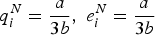
Equation (4) says that, in the absence of any environmental regulation, production leads to q i units of emissions (i.e., e i = q i). Therefore, firm i will not abate any pollution.Footnote 4 The profit maximization problem (3) allows us to determine the level of emissions E t before the adoption of the new environmental policy, that is,
 $$E^N = e_1^N + e_2^N.$$
We assume that the regulatory goal is to limit the quantity of industry emissions at some level E A by means of one of the following four environmental policy instruments: emissions taxes, standards, freely allocated tradable permits and auctioned permits. To make instruments directly comparable we assume that, in the initial situation, the level of emissions is the same under all four regimes. We assume that the environmental regu-lator has determined the Pigouvian tax (ζ) that equates the marginal benefits and costs of pollution.Footnote 5 The emission target E A is then assumed to be equal to the amount of emissions that the firms will produce, given this tax rate. Assuming that the tax rate is exogenously given, we are able to find the optimal emission level which is used as a benchmark for reduction of emissions and compare all four policy instruments. In section 4.2, we also relax this assumption when we suppose that the regulator uses the revenues accrued to finance public abatement activities. Hence, the objective of the environmental regulator is to cap the aggregate level of emissions at E A, either by establishing standards for firms or by issuing tradable permits to be distributed gratis or auctioned off. Under emission standards, firms' emissions are limited to  $\bar{e}_{1}$ and
 $\bar{e}_{2}$ respectively, such that
 $\bar{e}_{1} + \bar{e}_{2} = E^{A}$. Under a permits system, a total number of E A permits is either distributed freely, or auctioned off.
3.3. Taxes
In this section we compute the firm's operating profit under taxes and determine the level of emissions E A which serves as a benchmark for the reduction of emissions. Under tax regulation and Cournot competition, each firm looks for the output and the mix of abatement plus tax payment that maximizes profits. If the environmental regulator has decided to charge a per-unit fee equal to ζ, then firm i will maximize the following profit function:
 $$\left(\pi_i^A \right)^{Taxes} = \max_{e_i\comma q_i} \left\{p\lpar Q\rpar q_i - c_i\lpar q_i - e_i\rpar ^2 - \zeta e_i \right\}\comma \; \quad {\rm for}\, i = 1\comma \; 2.$$
The optimal level of emissions and output for each firm is given by the FOCs for e i and q i:
 $$2c_i\lpar q_i - e_i\rpar = \zeta\comma \;$$
 $$p\lpar Q\rpar + p^{\prime} \lpar Q\rpar q_i - 2c_i \lpar q_i - e_i\rpar = 0.$$
Equation (7) indicates that, at the optimum, each firm faces a marginal abatement cost equal to the emission tax ζ. Combining the FOCs for e i and q i, we have:
 $$p\lpar Q\rpar + p^{\prime }\lpar Q\rpar q_{i} = \zeta.$$
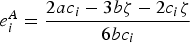
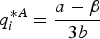
The term on the left-hand side in equation (8) is the marginal benefit of production, while the term on the right-hand side is the marginal abatement cost. At the optimum, each firm faces a benefit per unit of output equal to the tax ζ. Denoted by q iA and e iA are the optimal levels of output and emission under taxes of firm i. Notice that e iA < e iN for any level of ζ. Substituting (q iA, e iA) into (6), we obtain firm i's profit 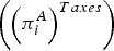 $\left(\left(\pi_i^A \right)^{Taxes} \right)$.Footnote 6 The aggregate level of emissions E t which serves as a benchmark for reduction of emissions is E A = e 1A + e 2A.
3.4. Emission standards
Under emission standards regulation and Cournot competition, the firms will maximize the following profit function:
 $$\left(\pi_i^A \right)^{Standards} = \max_{q_i} \left\{p\lpar Q\rpar q_i - c_i\lpar q_i - e_i\rpar ^2 \right\}\comma \;$$
subject to  $e_i\leq \bar{e}_i$ where
 $\bar{e}_i$ is the emission standard established for firm i. Setting
 $e_i=\bar{e}_i$, we assume that the emission standard is equal to the amount of emission that the firm produces under taxes (e iA). The optimal level of output for each kind of firm is given by the FOC for q i:
 $$p\lpar Q\rpar + p^{\prime} \lpar Q\rpar q_i - 2c_i \lpar q_i - e_i^A\rpar = 0.$$
The third term of (9) indicates that the environmental regulation raises marginal production costs by an amount equal to the marginal abatement cost at e i = e iA, which depends on the tax ζ. Substituting e iA into (9) and solving the resulting term for q i, we obtain firm i's best response function under emission standards q iA and then i's optimal profit (πiA)Standards.Footnote 7 Since both q iA are the same under taxes and emission standards and both e iA are the same under taxes and emission standards too, it follows that  $\left(\pi_i^A \right)^{Taxes} < \left(\pi_i^A \right)^{Standards}$ for any level of ζ.
3.5. Permits
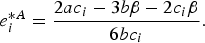
Under tradable permits regulation, each firm looks for the output and the mix of abatement plus emission permits that maximize profits. Following Montero (Reference Montero2002a,Reference Monterob) and Coria (Reference Coria2009), freely allocated permits and auctioned permits can be analyzed within a unique framework. Denote by ɛi (>0) the quantity of permits received by firm i and by β the market clearing price of permits after a total of E A permits have been distributed gratis by the regulator.Footnote 8 If instead the E A permits are auctioned off, ɛi = 0 and both firms become buyers of permits.Footnote 9
Under permits regulation, the firms will maximize the following function:
 $$\left(\pi_i^A \right)^{Permits} = \max_{e_i\comma q_i} \left\{p\lpar Q\rpar q_i - c_i\left(q_i - e_i \right)^2 - \beta \left(e_i - \varepsilon_i \right)\right\}.$$
The optimal level of emissions and production for each firm is given by the FOCs for e i and q i:
 $$2c_i\lpar q_i - e_i\rpar = \beta\comma \;$$
 $$p\lpar Q\rpar + p^{\prime} \lpar Q\rpar q_i - 2c_i \lpar q_i - e_i\rpar = 0.$$
Equation (11) indicates that, at the optimum, each firm faces a marginal abatement cost equal to the permit price β. Combining the FOCs for e i and q i, we have:
 $$p\lpar Q\rpar + p^{\prime} \lpar Q\rpar q_i = \beta.$$
The term on the left-hand side of Equation (12) is the marginal benefit of production, while the term on the right-hand side is the marginal abatement cost. At the optimum, each firm faces a benefit per unit of output equal to the permit price β.
The permits demand for each firm is obtained from (11):
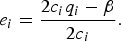 $$e_i = {2c_i q_i - \beta \over 2c_i}.$$
The market clearing condition requires total demand to be equal to total supply:
 $$e_1 + e_2 = E^A\comma \;$$
where E A is equal to the total amount of emissions that the firms will produce under taxes. The optimal levels of output and emissions of the two firms can be obtained from (12) and (13), and then also profits, (πiA)Permits. By comparing expressions (7) and (11) we get:
 $$\beta =\zeta.$$
That is, the market clearing price of permits is equal to the emission tax ζ.Footnote 10
Notice that, if permits are auctioned off (i.e., ɛi = 0), the operating profit (πiA)Permits is equal to the operating profits under taxes, while if permits are distributed freely (i.e., ɛi > 0) the operating profit (πiA)Permits is greater than the operating profits under taxes (since firms can gain from permits trading). Finally, note that the operating profit under auctioned permits is smaller than the operating profit under emission standards for any level of ζ (since the operating profit under auctioned profits is equal to the operating profit under taxes) while the operating profit under freely allocated permits is larger than the operating profit under emission standards if e iA < ɛi.
4. The regulator's problem
In this section we analyze the behavior of the regulator and the optimal stopping problem under each instrument. First, we consider the case in which the government revenues generated by pollution taxes and auctioned permits are redistributed to the firms and the consumers. Then, we examine an alternative fiscal policy decision and assume that the collected revenues are used to finance pollution abatement activities.
4.1. The optimal stopping problem under each policy instrument and revenue distribution
Using v (v = T, S, P Fr and P Au) to denote the policy regime (i.e., taxes, emission standards, freely allocated tradable permits and auctioned permits, respectively), in each period the regulator is supposed to decide whether to adopt the new environmental policy v or to postpone it to the next period.
Like Pindyck (Reference Pindyck2000), we assume that the flow of social costs (i.e., damages) associated with the stock variable M t is measured by the linear function:
 $$D\lpar \theta_t\comma \; M_t\rpar = \theta_t M_t\comma \;$$
where θt is a variable that stochastically shifts over time to reflect the damage due to the pollutant and is assumed to follow a geometric Brownian motion:
 $$d\theta _t = \alpha \theta _t dt + \sigma \theta_t dz_t\comma \; \theta_0 = \theta$$
for constants α < r, σ > 0, dz t is the increment of a standard Wiener process and r denotes the risk-free rate of interest. The process θt is assumed to capture economic uncertainty over future costs and benefits of policy adoptions. For example, changes in θt might reflect the innovation of technologies\ that would reduce the damage from a pollutant, or a change in the society's environmental sensitivity that would increase the social cost of M t. The linearity of D(θt, M t) is convenient because it makes the optimal policy independent of the stock M t. As suggested by Pindyck (Reference Pindyck2000, Reference Pindyck2002), for many environmental problems the damage from a pollutant is likely to rise more than proportionally with the stock of the pollutant. In the quadratic case, however, the well-established exponential term which accounts for the general solution (or option term) of the model does not guarantee uniqueness (this is proved in Framstad, Reference Framstad2011). Thus, our model would not admit a closed-form solution in the case of quadratic environmental cost and hence an appropriate numerical method is called for. Ecological uncertainty in the form of Ornstein–Uhlenbeck processes could also be factored into the analysis, but also in this case the model would not admit a closed-form solution. The projection method already studied by Balikcioglu et al. (Reference Balikcioglu, Fackler and Pindyck2011) seems suitable for this purpose.
Let B(θt, M t) denote the net benefit from emissions, i.e., the sum of consumer surplus (CS) plus the total profits earned by the firms (Π) plus the government revenue generated by each policy instrument (RV) minus the environmental damage due to the firms' production, D. If the regulator adopts the policy v, the net benefit is:
 $$\eqalign{B_v^A\lpar \theta_t\comma \; M_t\rpar & =CS^A + \left(\Pi^A\right)_v + \left(RV^A \right)_v \cr & \quad -D^A \lpar \theta_t\comma \; M_t\rpar \comma \; \quad {\rm for}\, v = T\comma \; S\comma \; P^{Fr}\, {\rm and}\, P^{Au}}$$
where (ΠA)v = (π1A)v + (π2A)v is the aggregated profit under each policy instrument. Given the demand curve p(Q), the consumer surplus CS A is equal to 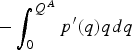 $-\int_{0}^{Q^{A}}p^{\prime }\lpar q\rpar qdq$, where
 $Q^{A}=q_{1}^{A}+q_{2}^{A}$ is the aggregate quantity in the presence of intervention. It equals
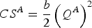 $CS^A={b\over 2}\left(Q^A\right)^2$ in the case of a linear demand function. The government revenue generated by each policy instrument is equal to:
 $$\left(RV^{A} \right)_{v} = \left\{\matrix{\zeta E^{A} \hfill &\hbox{if} v = T\comma \; P^{Au} \cr 0 \hfill &\hbox{if} v = S\comma \; P^{Fr}}. \right.$$
Both an emission tax and a system of auctioned permits generate government revenues (which equal the tax rate times the determined emission target under taxes), while emission standards and freely allocated permits do not generate any government revenue. The revenue from taxes and auctioned permits can be spent or redistributed to society. Here, we assume that the total tax (auction) revenue is completely redistributed to consumers and firms in a lump-sum fashion.
On the other hand, if the regulator never adopts the policy v, the net benefit is:
 $$B^{N} \left(\theta_{t}\comma \; M_{t} \right)= CS^{N} + \Pi^{N} - D^{N}\lpar \theta_{t}\comma \; M_{t}\rpar \comma \;$$
where  $\Pi ^{N} = \pi_{1}^{N} + \pi_{2}^{N}$ is the aggregated profit with no intervention, CS N = -∫0Q Np′ (q)qdq is the consumer surplus and Q N = q 1N + q 2N is the aggregate quantity in the absence of intervention. Here RV N = 0, because there is no public revenue in the absence of the regulator's intervention.
Let K v be the cost of permanently reducing the emission flows, v = T, S, P Fr and P Au. This cost is assumed to be completely sunk. The objective of the regulator is to choose the optimal timing of adopting policy v\ that would reduce emissions to E A such that the expected net present value function (using the discount rate r) of the difference between the net benefit  $B\left(\theta _{t}\comma \; M_{t}\right)$ and the cost of policy adoption K v, is maximized:
 $$W_{v}\lpar \theta\comma \; M\rpar = \sup_{\tau_{v} \in {\cal T}} {\open E} \left\{\left. \int\limits_{0}^{\infty }e^{-rt} B \left(\theta_{t}\comma \; M_{t} \right)dt - K_{v}e^{-r\tau_{v}} \right\vert {\cal F}_{0} \right\}\comma \;$$
subject to equation (1) for the evolution of M t and equation (15) for the evolution of θt. Here,  ${\cal T}$ is the class of admissible implementation times conditional to the filtration generated by the stochastic process θt. As usual, it is assumed that
 $r+\delta >\alpha $ for the integrability of the net benefit function
 $B\left(\theta_{t}\comma \; M_{t}\right).$
Applying the Dixit and Pindyck's (Reference Dixit and Pindyck1994) methodology, we can derive the optimal timing for the four environmental policies and the values to reduce emissions under the four environmental policies (see online appendix). In particular, we can compute the critical threshold  $\hat{\theta}_{v}$, v = T, S, P Fr and P Au such that it is optimal to adopt policy v for
 $\theta > \hat{\theta}_{v}$, with:
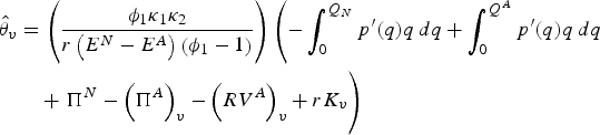 $$\eqalign{\hat{\theta}_{v} & =\left({\phi_{1}\kappa_{1} \kappa_2 \over r\left(E^{N} - E^{A} \right)\left(\phi_{1} - 1 \right)} \right)\left(- \int_0^{Q_N} p^{\prime} \lpar q\rpar q\, dq + \int_{0}^{Q^A} p^{\prime} \lpar q\rpar q\, dq \right. \cr &\quad + \left.\vphantom{\int_{0}^{Q^{A}}} \Pi ^{N}-\left(\Pi ^{A}\right)_{v}-\left(RV^{A}\right)_{v}+rK_{v}\right)}$$
where κ1 = r − α, κ2 = r + δ− α and ϕ1 is the positive solution to the standard characteristic equation.
In order to find a ranking of the four policy options, let us suppose first that all instruments require the same investment cost K. Moreover, we assume that the sunk cost of the policy implementation is a quadratic function of the amount that emissions are reduced:
 $$K\left(E^{N} - E^{A} \right)= h_1 \left(E^{N} - E^{A}\right)+ h_2 \left(E^N - E^A \right)^{2}\comma \;$$
with h 1, h 2 ≥ 0. From a comparison among the critical thresholds  $\hat{\theta}_{v}$ and among the welfare functions W v, we can get the following main results:
Proposition 1
The optimal adoption thresholds under taxes, auctioned permits and emission standards are equivalent.
Proposition 2
The value of the welfare functions W under taxes, auctioned permits and emission standards are equivalent.
Proof: of Propositions 1 and 2: in the online appendix.
Propositions 1 and 2 are a straightforward consequence of the following facts: (i) the (aggregated) profit under auctioned permits is equal to the profit under taxes, and (ii) the (aggregated) profit under emission standards is equal to the profit under taxes plus the revenue generated by the policy instrument, as shown in the online appendix. One clearly observes this by comparing the critical thresholds and the value of the options to reduce emissions under taxes, auctioned permits and emission standards.
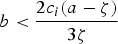
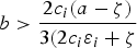
For the following, let us specify the model with a linear demand curve, p(Q) = a − bQ, where a, b > 0. Let  $b^{\ast} = {4c_{1}c_{2}\lpar a - \zeta \rpar \over 3\lpar c_{1}\lpar 2c_{2}\lpar \varepsilon_1 + \varepsilon_{2}\rpar + \zeta \rpar + c_{2}\zeta\rpar }$ be the critical value of the slope of market demand that makes the regulator indifferent between adopting emission standards and freely allocated permits. From a comparison between the thresholds
 $\hat{\theta}_{S}$ and
 $\hat{\theta}_{P^{Fr}}$ and between the welfare functions W S and W P Fr, we can get the following main results:
Proposition 3
The optimal adoption threshold under freely allocated permits is larger than the adoption threshold under emission standards (or auctioned permits or taxes) for 0 < b < b*. The optimal adoption threshold under emission standards (or auctioned permits or taxes) is larger than the adoption threshold under freely allocated permits for b > b*.
Proposition 4
The value of the welfare function W under freely allocated permits is smaller than the value of the welfare function W under emission standards (or auctioned permits or taxes) for 0 < b < b*. The value of the welfare function W under freely allocated permits is larger than the value of the welfare function W under emission standards (or auctioned permits or taxes) for b > b*.
Proof: of Propositions 3 and 4: in the online appendix.
Corollary
The values of the options to reduce emissions under taxes, auctioned permits and emission standards are equivalent. The value of the option to reduce emissions under freely allocated permits is smaller than the value of the option to reduce emissions under emission standards (or auctioned permits or taxes) for 0 < b < b*. The value of the option to reduce emissions under freely allocated permits is larger than the value of the option to reduce emissions under emission standards (or auctioned permits or taxes) for b > b*.
Propositions 3 and 4 are a straightforward consequence of the fact that the (aggregated) profit under emission standards is larger than the operating profit under freely allocated permits for 0 < b < b*, while for b > b* the operating profit under freely allocated permits is larger than the operating profit under emission standards (see online appendix). Since the level of emissions (for any value of b) is the same under all four policy options, so is the damage caused by the activity of production. Therefore, the comparison between emission standards (or auctioned permits or taxes) and freely allocated permits depends ultimately on the market price elasticity. If the output demand is more elastic (b smaller), then freely allocated permits offer smaller incentives than emission standards (or auctioned permits or taxes); alternatively, if it is more inelastic (b larger), then the reverse is true. Thus, Propositions 1, 2, 3 and 4 provide us with a ranking between taxes, emission standards, auctioned permits and freely allocated permits in this setting, in a non-equivocal way. It is found that emission standards, emission taxes and auctioned permits are more conducive to early adoption than freely allocated tradable permits for 0 < b < b*. Regulators may care about early adoption: in this case, emission standards, taxes and auctioned permits outperform freely allocated permits, i.e., they should be the preferred policy instrument. Contrarily, for b > b* freely allocated permits are more conducive to early adoption than emission standards, taxes and auctioned permits.
Remark 1
Proposition 1 states that the optimal adoption thresholds under taxes, auctioned permits and emission standards are equal if the cost of each policy is equal. If the cost of permanently reducing the emission flows, K v, differs among the different policies, v = T, S, P Fr and P Au, then, in view of the fact that the optimal adoption thresholds under taxes, auctioned permits and standards are increasing in the cost K v, we get  $\hat{ \theta}_{v}>\lpar <\rpar \hat{\theta}_{w}$ if K v > (<) K w, where
 $v\comma \; w = T\comma \; S\comma \; P^{Au}$, v ≠ w. That is, ultimately the regulator needs to consider the cost of policy.
Remark 2
If the cost of permanently reducing the emission flows, K v, differs among the different policies, v = T, S, P Fr and P Au, then, in view of the fact that the optimal adoption thresholds under freely allocated permits and standards are increasing in the cost K v, we get that the optimal adoption threshold under freely allocated permits is larger (smaller) than the adoption threshold of emission standards if  $K_{P^{Fr}}>K_{S}$, for b < b* (
 $K_{P^{Fr}}<K_{S}$, for b > b*).
4.2 The optimal stopping problem with public spending in abatement activities
We now analyze the optimal stopping problem when the government revenues generated by pollution taxes and auctioned permits are used to finance pollution abatement activities, e.g., abatement of water pollution, air pollution and, more generally, policies that protect natural resources. Such policies are costly and a major conviction is that public finance should play a role in meeting such requirements (see also European Commission Environment Policy Review, available at http://ec.europa.eu/environment/policyreview.htm).
Pollution taxes generate ζ E A revenues. Suppose that the government decides to use these revenues to finance pollution abatement activities. Assuming a balanced budget, we have:
 $$GS = \zeta E^{A}$$
where GS denotes government spending. Under emission standard regulation, firms' emissions are limited to the quantity of emissions that the firms will produce under taxes. Hence, in this situation there are neither public revenues nor pollution abatement activities, i.e., GS = 0.
Finally, under a tradable permits system, a total number of E A permits are either distributed freely or auctioned off. Hence, the government spending is equal to GS = ζ E A if permits are auctioned off and GS = 0 if permits are distributed freely.
It is reasonable to modify the pollution dynamics in the adoption region in the following way:
 $$dM_{t} = \left(E^{A} - f \left(GS \right)- \delta M_{t} \right)dt\, \hbox{for}\, t \geq \tau$$
where f is an increasing and concave function, such that f(0) = 0. Under this assumption, the speed of pollution accumulation is reduced by a factor  $ f\left(GS\right)$ which measures the environmental benefits associated with the government spending on pollution abatement activities. It is helpful to rewrite equation (2) as follows
 $$dM_{t} = \left\{\matrix{\left(E^{N} - \delta M_{t} \right)dt \hfill &\hbox{for}\, 0 \leq t < \tau_{v} \hfill \cr \left(E^{A} - g_{v} - \delta M_{t} \right)dt \hfill &\hbox{for}\, t \geq \tau_{v}\comma \; \hfill}\comma \; \right.$$
where  $g_{v} = f \left(GS \right)>0$ if v = T, P Au and g v = 0 if v = S, P Fr. In such a framework there is more abatement with taxes and auctioned permits than with emission standards or freely allocated permits for 0 < ζ< 1.
Let 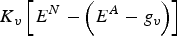 $K_{v}\left[E^{N}-\left(E^{A}-g_{v}\right)\right]$ be the (sunk) cost of permanently reducing the emission flows, which is given by:
 $$K_{v}\left[E^{N}-\left(E^{A}-g_{v}\right)\right]=h_{1}\left[E^{N}-\left(E^{A}-g_{v}\right)\right]+h_{2}\left[E^{N}-\left(E^{A}-g_{v}\right)\right]^{2}\comma \;$$
with h 1, h 2 ≥ 0. Here the cost of permanently reducing emission flows is larger under taxes and auctioned permits than under emission standards and freely allocated tradable permits. It is also in keeping with some empirical evidence, where emission standards and freely allocated permits are easier to be implemented and require smaller organizational and administrative costs.
As before, the net benefit in the absence of intervention is  $B^{N}\left(\theta_{t}\comma \; M_{t} \right)= CS^{N} + \Pi^{N} - D^{N}\lpar \theta_{t}\comma \; M_{t}\rpar $ while
 $B_{v}^{A} \left(\theta_{t}\comma \; M_{t} \right)= CS^{A} + \left(\Pi^{A} \right)_{v} - D^{A} \lpar \theta _{t}\comma \; M_{t}\rpar $ is the net benefit in the presence of the regulator's intervention. Notice that environmental revenues are not included in
 $B_{v}^{A}\left(\theta_{t}\comma \; M_{t}\right)$ since they are completely used to finance public abatement. The regulator solves the stopping problem (16) to choose the optimal timing of adopting policy v that would reduce emissions to E A − g v such that the expected net present value function of the difference between the net benefit
 $B\left(\theta_{t}\comma \; M_{t}\right)$ and the cost of policy adoption
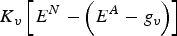 $K_{v}\left[E^{N}-\left(E^{A}-g_{v}\right)\right]$, is maximized.
Following the same calculation as before, we can derive the optimal thresholds for each policy instrument. In particular, we can compute the critical threshold  $\tilde{\theta}_{v}$, v = T, S, P Fr and P Au\ such that it is optimal to adopt policy v for
 $\theta >\tilde{\theta}_{v}$, with:
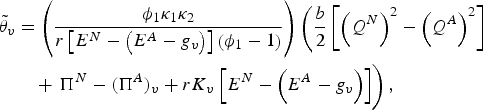 $$\eqalign{\tilde{\theta}_{v}&=\left({\phi_{1}\kappa_{1}\kappa_{2} \over r\left[E^{N} - \left(E^{A} - g_{v}\right)\right]\left(\phi_{1} - 1 \right)} \right)\left({b \over 2} \left[\left(Q^{N}\right)^{2} - \left(Q^{A} \right)^{2}\right]\right. \cr &\quad + \left.\vphantom{\left[\left(Q^{N}\right)^{2}-\left(Q^{A}\right)^{2}\right]} \Pi^{N} - \lpar \Pi ^{A}\rpar _{v} + rK_{v} \left[E^{N} - \left(E^{A} - g_{v}\right)\right]\right)\comma \; }$$
where  $g_{v} = f \left(GS \right)$ if v = T, P Au and g v = 0 if v = S, P Fr. From a comparison between the thresholds
 $\tilde{\theta}_{T}$ and
 $\tilde{\theta}_{P^{Au}}$ and between the welfare functions W T and
 $W_{P^{Au}}\comma \; $ we can get the following main results:
Proposition 5
Assuming that the collected revenues are used to finance pollution abatement activities: (i) the optimal adoption threshold under taxes is the same as the optimal adoption threshold under auctioned permits; (ii) the value of the welfare function W under taxes is the same as the value of the welfare function W under auctioned permits.
Moreover, from a comparison between the thresholds  $\tilde{\theta}_{S}$ and
 $\tilde{\theta}_{P^{Fr}}$ and between the welfare functions W T and
 $W_{P^{Au}}\comma \; $ we can get the following main results:
Proposition 6
Assuming that the collected revenues are used to finance pollution abatement activities: (i) the optimal adoption threshold under freely allocated permits is larger than the adoption threshold under emission standards for 0 < b < b*; (ii) the optimal adoption threshold under emission standards is larger than the adoption threshold under freely allocated permits for b > b*.
Proposition 7
Assuming that the collected revenues are used to finance pollution abatement activities: (i) the value of the welfare function W under freely allocated permits is smaller than the value of the welfare function W under emission standards for 0 < b < b*; (ii) the value of the welfare function W under emission standards is smaller than the value of the welfare function W under freely allocated permits for b > b*.
Propositions 5, 6 and 7 can be proved following the same argument of Propositions 1, 2, 3 and 4.
Unfortunately, we cannot compare the critical thresholds under taxes and auctioned permits with the critical thresholds under emission standards and freely allocated permits, in our theoretical model. The reason is that there is more abatement with taxes and auctioned permits than with emission standards or freely allocated permits and hence the levels of emissions are different under the different policy instruments. However, numerical simulations allow us to compare the critical thresholds under taxes, emission standards and permits. This will help us to shed light on the possible rankings of the policy instruments under different specifications of the parameter values.
5. Simulation results
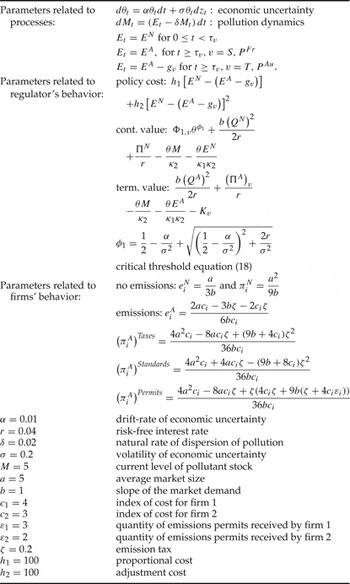
In this section we provide some numerical applications and sensitivity analysis for the social value function and the optimal thresholds under the alternative environmental policies for the reduction of emissions. The simulations are implemented using  $g_{v}=\left(GS\right)^{1 \over 2}$ if v = T, P Au and g v = 0 if v = S, P Fr. We use as much as possible the same parameter values as in Pindyck (Reference Pindyck2000) and Montero (Reference Montero2002a,Reference Monterob). The case b = 1 (considered here) corresponds to an inelastic demand case. Table 1 summarizes the models and the notations.
Base case parameters

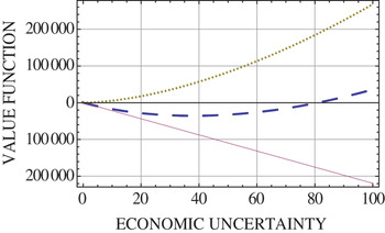
Figure 1 shows the relation between the social value function W S and the level of economic uncertainty θ.Footnote 11 The dashed curve refers to the value of the welfare function in the no-adoption region (or value of continuation), the solid curve to the value function in the adoption region minus the cost of policy adoption (or value of termination) and, finally, the dotted curve to the value of the option to adopt the policy,  $\Phi_{1\comma S} \theta^{\phi_1}$. We consider values of economic uncertainty θ ranging from 0 to 100. The critical threshold
 $\tilde{\theta}_{S}$ is found at the point of tangency of W SN with the line
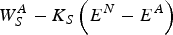 $W_{S}^{A}-K_{S}\left(E^{N}-E^{A}\right)$. We found
 $\tilde{\theta}_{S}\simeq 0.55$. For values of
 $0 < \theta < \tilde{\theta}_{S}$ the policy should not be adopted, while for
 $\theta \geq \tilde{\theta}_{S}$ the policy should be immediately adopted. At the optimal adoption threshold, the value of the option to implement the policy is about 41.5. We can compare our results with those obtained by Pindyck (Reference Pindyck2000:243). As M increases (and so the social cost of environmental damage), the social value functions in the no-adoption and in the adoption regions decrease (the curves shift downwards); however, the critical threshold
 $\tilde{\theta}_{S}$ is unaffected by M and so the optimal adoption policy is unchanged.
Relation between the social value function W SN and the level of economic uncertainty, θ (dashed curve). Relation between the termination value W SA − K S(E N − E A) and the level of economic uncertainty, θ (solid curve). Relation between the value of the option to adopt the policy and the level of economic uncertainty, θ (dotted curve).

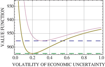
Figure 2 shows the relation between the social value function W v and the volatility of economic uncertainty σ. The dashed curves refer to the values of termination under freely allocated permits and emissions standards while the solid curves refer to the values of continuation  $W_{v}^{N}\comma \; v=S\comma \; P^{Fr}.$ The values of termination are neutral to variations in the volatility of economic uncertainty, hence they are depicted as straight lines with respect to σ. We consider values of the volatility σ ranging from 0 to 1 and values of the social benefit function at the critical threshold
 $\theta =\tilde{\theta}_{S}\simeq 0.55.$ At this point the option to reduce emissions under emissions standards is near exercise. However, the option to reduce emissions under freely allocated permits is already exercised since
 $\theta =\tilde{\theta}_{P^{Fr}}\simeq 0.37$ is the critical threshold for exercising freely allocated permits. Note indeed that, since
 $b^{\ast }\cong 0.63\comma \; $ the regulator will prefer freely allocated permits to emission standards when b = 1 as suggested by Propositions 6 and 7 (see also in connection to figure 5). Hence, the upper dashed line refers to the value of social welfare in the no-adoption under emissions standards. The continuation value
 $W_{S}^{N}$ is greater than the continuation value
 $W_{P^{Fr}}^{N}$ because the option value under freely allocated permits is lost due to the exercise. In the same way, we can compare the value functions under emissions standards and under taxes (or auctioned permits). However, in this case the critical threshold
 $\theta =\tilde{\theta}_{v}\simeq 0.81\comma \; v=T\comma \; P^{Au}$, hence the option has not been exercised and does have value; the continuation value
 $W_{v}^{N}\comma \; v=T\comma \; P^{Au}$ is greater than the continuation value
 $W_{S}^{N}$ at the point
 $ \theta =\tilde{\theta}_{S}\simeq 0.55$.
Relation between the social value function W SN and the volatility of economic uncertainty, σ (upper solid curve). Relation between the social value function W p FrN and the volatility of economic uncertainty, σ (lower solid curve). Relation between the values of termination and the volatility of economic uncertainty, σ (dashed curves).

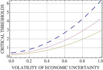
Figure 3 shows the relation between the critical threshold  $\tilde{\theta} _{v}$, v = T, S, P Fr and P Au and the volatility σ. The dashed curve refers to the critical threshold under taxes, the solid curve to emission standards and the dotted curve to freely allocated tradable permits. We recall that the critical threshold under taxes coincides with the critical threshold under auctioned permits. We consider values of the volatility σ ranging from 0 to 1. As in Pindyck (Reference Pindyck2000), the critical thresholds are upward sloping with respect to σ. The reason is that an increase of economic uncertainty over future payoffs from reduced emissions increases the value of waiting and raises the critical threshold
 $\tilde{\theta}_{v}$. The simulation provides us with a ranking between taxes, emission standards, freely allocated tradable permits and auctioned permits (in terms of their adoption lag) when σ increases. We observe that the critical threshold under taxes and auctioned permits is larger than the critical thresholds under emissions standards and auctioned permits; moreover, it is found that the critical threshold under freely allocated permits is lower than the critical thresholds under emissions standards, taxes and auctioned permits. That means that freely allocated permits are more conducive to early adoption than emission taxes, emission standards and auctioned permits in this base case.
Relation between the critical thresholds  $\tilde{\theta}_{\tau}$ and
 $\tilde{\theta}_{p^{Au}}$ and the volatility of economic uncertainty σ (dashed curve). Relation between the critical threshold
 $\tilde{\theta}_S$ and the volatility of economic uncertainty σ (solid curve). Relation between the critical threshold
 $\tilde{\theta}_{p^{Fr}}$ and the volatility of economic uncertainty σ (dotted curve).

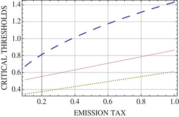
Figure 4 shows the relation between the critical threshold  $\tilde{\theta} _{v}$, v = T, S, P Fr and P Au and the emission tax ζ. The dashed curve illustrates the sensitivity of the critical threshold under taxes, the solid curve under emission standards and the dotted curve under freely allocated tradable permits. We consider values of the emission tax ζ ranging from 0.1 to 1. The critical thresholds are upward sloping with respect to ζ. The reason is that a higher ζ reduces firms' profits and thus necessitates a higher θ for the investment in reduced emissions to take place. The intuition is as follows. The optimal implementation time is defined as that level of θ at which the continuation and the termination values are equal. Evaluating both values at
 $\tilde{\theta}_{v}$ and increasing the level of stringency of environmental policy increases both the continuation and the termination values (the curves shift upwards). Indeed, a larger ζ would reduce the level of emission flow and reduce the social cost of environmental damage (this shifts the curves of termination upwards) and hence increase the value of the option to implement the environmental policy. Moreover, higher levels of environmental stringency render the firm's economic activity less profitable, and hence reduce the value of the option to implement the environmental policy (which would reduce social damage) in the future; overall, the effect on firm's profits seems to dominate. That means that, when faced with a more stringent environmental policy, the continuation value associated with the emissions level E N is larger than its termination value with abated emissions, and hence the regulator will decide to wait longer to adopt the new environmental policy v.
Relation between the critical thresholds  $\tilde{\theta}_{\tau}$ and
 $\tilde{\theta}_{p^{Au}}$ and the emission tax ζ (dashed curve). Relation between the critical threshold
 $\tilde{\theta}_{S}$ and the emission tax ζ (solid curve). Relation between the critical threshold
 $\tilde{\theta}_{p^{Fr}}$ and the emission tax ζ (dotted curve).

The result that the more stringent the policy, the more firms would delay the adoption of lower emission policies, was also highlighted in Van Soest (Reference Van Soest2005), however, using a different model with a different objective function. Also Agliardi and Sereno (Reference Agliardi and Sereno2011) obtain the same sensitivity results with respect to the stringency of environmental policy, although permits and public expenditures are not taken into account.
It is found that the critical threshold under taxes and auctioned permits is larger than the critical thresholds under emissions standards and freely allocated permits. Moreover, it is found that the critical threshold under freely allocated permits is lower than the critical thresholds under taxes, emissions standards and auctioned permits. As in the previous case, freely allocated permits are more conducive to early adoption than emission taxes, emission standards and auctioned permits.
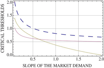
Figure 5 shows the relation between the critical threshold  $\tilde{\theta}_{v}$, v = T, S, P Fr and P Au and the slope of the market demand b. The dashed curve refers to the critical threshold under taxes and auctioned permits, the solid curve to emission standards and the dotted curve to freely allocated tradable permits. We consider values of b ranging from 0.1 (elastic output demand case) to 2 (inelastic output demand case). The critical thresholds are downward sloping with respect to b. The reason is that a higher b would reduce the level of emission flow and reduce the social cost of environmental damage and thus necessitates a lower θ for the investment in reduced emissions to take place. The intuition is as follows. In the Cournot game the level of output depends inversely on the price elasticity. As the output demand is more inelastic the level of emissions is lower and the firm's economic activity is less profitable; the continuation and termination curves shift downwards. Also the option to implement the environmental policy (which would reduce social damage) in the future is less valuable. That means that, when faced with a more inelastic output demand, the continuation value associated with the emissions level E N is lower than its termination value with emission level E A − g v, and hence the regulator will decide to speed up the adoption of the new environmental policy v.
Relation between the critical thresholds  $\tilde{\theta}_{\tau}$ and
 $\tilde{\theta}_{p^{Au}}$ and the slope of the market demand b (dashed curve). Relation between the critical threshold
 $\tilde{\theta}_{S}$ and the slope of the market demand b (solid curve). Relation between the critical threshold
 $\tilde{\theta}_{p^{Fr}}$ and the slope of the market demand b (dotted curve).

The numerical simulation provides us with a ranking between taxes, emission standards, freely allocated tradable permits and auctioned permits, in terms of their adoption lag, when b increases. It is found that: (i) the critical threshold under taxes and auctioned permits is larger than the critical thresholds under emissions standards and freely allocated permits; (ii) the critical threshold under freely allocated permits is larger than the critical threshold under emission standards for values of b ranging between 0.1 and about 0.63, while the critical threshold under emission standards is larger than the critical threshold under freely allocated permits for values of b greater than about 0.63. Thus, the regulator is indifferent between adopting emission standards and freely allocated permits when b≅ 0.63. The regulator will prefer emission standards to freely allocated permits when the value of b ranges between 0.1 and (about) 0.63. And finally the regulator will prefer freely allocated permits to emission standards when the value of b is greater than (about) 0.63.
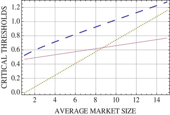
Figure 6 shows the relation between the critical threshold  $\tilde{\theta} _{v}$, v = T, S, P Fr and P Au and the average market size a. The dashed curve refers to the critical threshold under taxes and auctioned permits, the solid curve to emission standards and, finally, the dotted curve to freely allocated tradable permits. We consider values of a ranging from 1 to 15. It is found that freely allocated permits are more conducive to early adoption than taxes, emission standards and auctioned permits for values of a ranging between 1 and 7.7875, while for values of a greater than 7.7875 emission standards are more conducive to early adoption than taxes, emission standards and auctioned permits.
Relation between the critical threshold thresholds  $\tilde{\theta}_{\tau}$ and
 $\tilde{\theta}_{p^{Au}}$ and the average market size a (dashed curve). Relation between the critical threshold
 $\tilde{\theta}_{S}$ and the average market size a (solid curve). Relation between the critical threshold
 $\tilde{\theta}_{p^{Fr}}$ and the average market size a (dotted curve).

In conclusion, our findings are that the critical threshold under taxes and auctioned permits is always larger than the critical thresholds under emissions standards and auctioned permits. The reason is that taxes and auctioned permits require higher costs of implementation and therefore the termination value associated with emission level 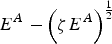 $E^{A}-\left(\zeta E^{A}\right)^{1 \over 2}$ is lower than the termination value associated with the emission E A. When we compare the termination values with the continuation values, results show that at the optimal adoption time the critical thresholds under emission standards and freely allocated permits are lower than the critical thresholds under taxes and auctioned permits. Hence, emission standards and freely allocated permits are preferred to taxes and auctioned permits if the regulator aims at speeding up the adoption of pollution-reducing policies. Moreover, comparing the critical thresholds under emission standards and freely allocated permits we find that emission standards are preferred to freely allocated permits when the output demand is more elastic, while freely allocated permits are preferred if the output demand is more inelastic. This result is in contrast with Coria (Reference Coria2009) where a different ranking is found. In particular, Coria (Reference Coria2009) shows that, if the regulator wants to speed up technological diffusion (i.e., firms adopting pollution reducing technology), auctioned permits are preferred to freely allocated permits and taxes when the output demand is more elastic. Her model, however, considers a different case where a policy is adjusted in response to the availability of a new technology.
6. Conclusion
This paper is about the optimal timing of a new environmental policy in a framework where production causes pollution, economic volatility is the main source of uncertainty, competing firms are regulated by taxes, emission standards, auctioned permits or freely allocated permits and the government is concerned with the finance requirements of the environmental protection. In particular, two possible fiscal policy decisions are considered: either the government revenues generated by pollution taxes and auctioned permits are redistributed to the firms and the consumers, or the collected revenues are used to finance pollution abatement activities.
Our main results concern the rankings of the alternative policy options in terms of their adoption lag and social welfare. We show that when the output demand is elastic, emission standards are preferred to freely allocated permits. Alternatively, if demand is inelastic, freely allocated permits provide more incentives than taxes, emission standards and auctioned permits. Taxes and auctioned permits are always equivalent in terms of their adoption lag and social welfare and also equivalent to emission standards when the regulator redistributes revenues and the cost of the policy implementation is the same among the policies.
Our paper contributes to the recent debate in the literature by discussing the impact of these alternative policy instruments on the optimal timing of emission reductions. Environmental protection and the timing of policy intervention have become a priority and indeed a challenge for many governments. In our model there is an unambiguous ranking of these policy instruments in terms of the adoption lags: if regulators wish to speed up the implementation of technologies reducing pollution emissions, then they may prefer standards to taxes or permits if demand is rather elastic. This result is robust to the two fiscal policies adopted and to various relevant parameters. Therefore, our sensitivity analysis provides a clue to regulators who are faced with environmental issues where economic costs and benefits cannot be forecasted and a lot of scenarios can be considered. An interesting extension is to examine the effects of asymmetric information among actors in the economy, for example, the effects of signaling on environmental policies where each firm privately knows whether its technology is clean or not, while third parties (i.e., the regulator) have only a subjective perception about it. We leave such issues for future research.