1. INTRODUCTION
The design process is a sequence of phases from the definition of needs and requirements to preliminary design and detailed design (Pahl & Beitz, Reference Pahl and Beitz1996). Preliminary design includes conceptual design (CD) and embodiment design (ED). The ED phase investigates the feasibility of some product schemes obtained from the CD phase. This phase mainly tackles physics behaviors and interactions between the product, its components, and environments. Product modeling is based on the definition of the laws of physics, functional models, economic criteria, and so forth.
In this paper we focus on robust ED taking into account variability, uncertainty, or imprecision in the design process. The goal is to determine the main structuring characteristics of a product, such as the working structure, standard components, and the main dimensions, whereas no significant decisions have been taken at that point. Several components may change during this phase. Robust ED can be implemented in a constraint-based approach. Product models can be translated into numerical constraints. Uncertainty and imprecision can be partially captured by interval computations. Heterogeneous models and incomplete information can naturally be dealt with. These models are involved in robust design approaches taking into account mathematical models during the early phases of design process. Robustness may be regarded through its meaning within the design community (Rothwell & Gardiner, Reference Rothwell, Gardiner and Oakley1990).
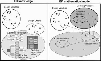
Product modeling leads to the definition of several types of constraints. Behavior laws relating to physics analysis concerning a product are expressed through conservation laws, which are easily translated into constraints. In some cases, behavior laws are defined by sets of phenomenological relations, namely, piecewise relations depending on one or several parameters. Product modeling also leads to the definition of several types of variables. Design variables are related to the main dimensions and characteristics of the product. Designers are interested in finding out powerful solution principles, where design variable values correspond to high-performance criteria. Performance criteria may be represented by performance variables. Other variables of the model are auxiliary variables, maintained within the model to link design variables to performance variables to preserve the model intelligibility. They are introduced by the modeling phase (see Fig. 1).
The variable kinds in the ED phase.

In this figure, the ED knowledge of a product takes into account design variables, which values identify each design solution. Designers use also several criteria to observe and evaluate the design solutions. Several diagrams and charts are used to identify the product functions and decomposition (technical organization charts) and to investigate the physics phenomena regarding fluxes and induced effects (fluxes flow diagram and substance field graph). In the modeling part of the ED phase, these concepts are translated into a mathematical representation. Obviously, the variables already defined in the knowledge representation are also in the mathematical model, and in most cases, criteria are easily expressed with constraints and some variables to observe criteria values. But diagrams and charts must be converted in a computable form. New variables are introduced, and they do not correspond to decision parameters used by designers. Thus, these new variables and constraints describe physics phenomena, products geometry characteristics, and so forth. Some functional variables are defined to preserve the model intelligibility and to express, for instance, well-known physics dimensionless numbers characterizing physics phenomena. Some of them are introduced after some steps of model reductions.
Our purpose is to define new constraint satisfaction techniques in the interval-based branch and prune framework to solve enriched models of ED applications. We investigate enriched robust ED models, because we consider various knowledge about products: specifications and requirements, knowledge of designers concerning the whole product life cycle, physics phenomena, and so forth. All this knowledge is required to compute quite safe and robust values (from a design point of view) for the main variables of an ED model. The first problem is to handle specific physics phenomena. To this end a global piecewise constraint is defined at the modeling and the solving levels. The second problem is to tackle the different types of variables. Existential quantifiers are introduced in the constraint-based model to take into account the fact that auxiliary variables are meaningless from a design point of view. New heuristics allow the differentiation of the variables during search, according to their types. An experimental study from a prototype and several benchmarks are reported. Complete models are given in the appendixes for people who want to make their own test with real-world applications.
Section 2 introduces CSP modeling for ED. Solving principles are presented and some search strategies are stated in Section 3. Experimentations on academic problems are carried out in Section 4. ED models derived from existing engineering models are processed in Section 5. Our approach is compared to some related work in Section 6.
2. PROBLEM MODELING
We consider ED problems defined as mixed models including integer variables, real variables, constraints, and piecewise constraints. The main idea of this paper is to distinguish between variables according to application requirements and to separate them in several sets during the search phase of solutions. A model is defined by a set X of variables lying in some domain D and a set of constraints C. Each constraint is a restriction of D given atomic formula over the usual structure of real numbers. Our goal is to find values in D for the variables of X satisfying all the constraints in C.
2.1. Types of variables
In ED problems, two types of variables are highlighted: the auxiliary variables, and the main variables including the design variables and the performance variables. The main variables must be computed at a given discernment precision. The values of the auxiliary variables may be useless from the designer's point of view; no initial precision or carefully chosen precision may be defined. The distinction between main variables and auxiliary variables is possible, because main variables are deduced by the product specifications and requirements. Most of the main variables are shared by all design phases. They identify the main characteristics of products; that's why their domains and precisions are well known, on the contrary, to the auxiliary variables, which are specific to each design phase.
Notation
Given a variable or a set of variables x, a real number or a set of real numbers r, and a constraint or a conjunction of constraints C on x, we write C(r) if C is satisfied when x has value r.■
Let X = (x 1, … , x n) denote the main variables, let Y = (y 1, … , y m) denote the auxiliary variables, and let D X and D Y be their domain. To solve ED problems may be seen as the computation of the set of solutions for the main variables, where there is at least one solution for auxiliary variables:

where C stands for the constraints to be satisfied.
In other words, the main variables define a scheme of solution for designers, namely, the main architectures of a product. The description of the product and its components (behavior, geometry, etc.) makes these architectures physically valid, if at least one solution is found on the auxiliary variables for each architecture.
Several approaches can be used to tackle such problems. Search problems may correspond to our ED problems, because solutions to ED problems are other than yes or no, contrary to decision problems. But it can be seen in Beame et al. (Reference Beame, Cook, Edmonds, Impagliazzo and Pitassi1995) that for each search problem an equivalent decision problem exists and in an ED context, it may be expressed as

where all variables are linked with an existential quantifier. Efficient SAT algorithms (Cook & Mitchell, Reference Cook and Mitchell1997) can be used in this case, but because an existential quantifier is applied to each variable, only one solution may be found to be the yes answer.
The constraint satisfaction problem (CSP) approach defines a framework for solving general problems expressed as a conjunction of constraints, where all variables are free:

All values r for variables satisfying C are computed. This approach does not match the formulation in (1), but the solving algorithms can be adjusted to undertake an existential quantifier on some variables.
Another type of variables has to be taken into account: functional variables (considering their mathematical meaning and not their design meaning). These variables are introduced by designers while modeling a product. They improve the expressivity and comprehensibility of a model, while expressing well-known characteristics about a product or its behavior. It allows designers to better handle and modify a model. Most of functional variables are expressed as a function of other variables:

where x is a functional variable, y a set of variables, and f(y) is an expression such as no variable in y is defined from x. A causal link can be established between a functional variable x and variables in y: they are used to compute its values. Functional variables can easily be removed from a model. Thus, an equivalent problem to solve is obtained by replacing their occurrences with their expression. Nevertheless, this new problem is difficult to manage, because most of the constraints become quite incomprehensible for designers and changings are hardly performed. Inserting these variables and their domain within a problem artificially increases the size of the search space. Exploring their domain may drastically penalize the solving process because consistent domains can explicitly be deduced from the evaluation of f(y). It must be highlighted that all equality constraints have not to be considered as a functional variable definition. The knowledge of designers and the way they build a model define which variables have to be considered as functional variables.
We implement our approach and its corresponding algorithms within a CSP framework that uses continuous domains. This framework is suitable for solving ED problems (Zimmer & Zablit, 2001; Gelle & Faltings, 2003; Vareilles et al., Reference Vareilles, Aldanondo, Gaborit and Hadj-Hamou2005). The CSP approach allows designers to make their models evolve very quickly as opposed to other methods, where designers express the knowledge, while carrying out its coding related to numerical solving methods similar to the constraint satisfaction approach. Some examples based on an evolutionary approach may be found in Sébastian et al. (Reference Sébastian, Chenouard, Nadeau and Fischer2006). Moreover, the solving process of a CSP guarantees the completeness of the set of approximate solutions, whereas other methods are often linked with relaxations and approximations of some stochastic solutions.
2.2. Interval computations and variable precision
The problem of computing solutions for functions on real numbers is known to be undecidable (Richardson, Reference Richardson1968; Wang, Reference Wang1974). Computers arithmetic (see IEEE 754 standard) defines a subset of real numbers, called the floating-point numbers. Without any other techniques, computations are made using floating-point numbers and rounding errors may be important after several computation steps.
Interval arithmetic (Moore, Reference Moore1966) guarantees safe computations using floating-point numbers as interval bounds. For each real number a, an interval hull(a) = [a −, a +] may be used, corresponding to the smallest interval including it, where a − is the highest floating-point number smaller than a and a + is the lowest floating-point number higher than a. Furthermore, every operator and function must be extended from real numbers to intervals with real bounds and then a hull with floating-point bounds is computed. For example, the three basic operators on real numbers can be extended as follows:
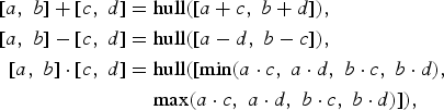
where hull([a, b]) = [a −, b +] and a − and b + are the closest floating-point numbers lower than a and upper than b.
Other Notations
Given a variable x, an interval I and a constraint C on x, we write C(I) if C is satisfied in the interval sense [see Section 2.3 and Eq. 6 for more details], when x takes value I. The size of an interval I = [a, b] is equal to w(I) = b − a. Given a set of real numbers A, the hull of A, denoted by hull(A), is the smallest interval enclosing A.■
Real values within intervals cannot be enumerated as values in discrete domains, but intervals are split to reduce their width because a smallest hull is computed or an interval precision is reached. A precision p(x) may be defined for a variable x. It defines the interval width, where we do not want any more computations to be done. The precision on variable domains can be interpreted as uncertainties about the computed values of some important variables. Moreover, the precision on domains of main variables referring to dimensions may also be viewed as tolerances. Precisions of auxiliary variables are often difficult to agree on. It must be highlighted that the set of auxiliary variables is often underconstrained, because, in the ED phase, some uncertainties remain about some product characteristics and its behavior. Physical phenomena are often complex and many simplifying assumptions are done. Some of them concern the context of the investigated life situations, whereas others come from a lack of knowledge about the product behavior and about the interfering phenomena.
Two types of precisions may be highlighted in ED. The precision on main variables corresponds to the precision of discernment of design architectures, whereas precisions on auxiliary variables define numerical precisions for computations. To define precisions on all types of variables may increase the efficiency of the computing process, because an interval precision is often achieved before the smallest hull (or canonical hull) of a real number.
Suppose that p(x k) ≥ 0 (the value 0 for a precision expresses the need of a canonical interval box for a variable) is the desired precision of x k (k = 1, … , n). We now consider the finite set of approximate solutions:

where I = I 1 × · · · × I n and J = J 1 × · · · × J m, such that I is precise enough, that is, w(I k) ≤ p(x k) for k = 1, … , n, and each interval bounds are floating-point numbers. The first goal is to compute a subset of (4) enclosing (1) having a minimal cardinal. To this end the main variable values must be close to their precisions, that is, w(I k) ≈ p(x k). The second goal is to prove the existence of a solution (element from set 1) in every resulting box. Proofs of existence can be implemented by interval analysis techniques, and this will be detailed in the next section.
2.3. CSP notions
A CSP is defined by three sets corresponding to a set X of variables, a set D corresponding to their domains and a set C of constraints restricting the variables values. The goal is to find every element of D that satisfies all constraints at the same time. This problem is unsolvable given continuous domains and transcendent functions. A more practical goal is to compute a finite approximation of the set of solutions (Lhomme, Reference Lhomme1993). The most common approach is to calculate a set of interval boxes of a given size enclosing the solution set.
The satisfaction of a numerical constraint is usually defined as follows: every variable is interval valued, every expression is evaluated using interval arithmetic (Moore, Reference Moore1966), and every relation between intervals is true whenever there exist reals within intervals that satisfy the following relation:

where C is the interval extension of the constraint c on reals (i.e., each variable is replaced by its interval domain and each function or operator is extended to the interval arithmetic).
The satisfaction of constraints is verified using consistency techniques. Variable domains are checked considering the whole set of constraints. If a domain is not consistent, then all unauthorized values (or intervals) are removed as long as they do not satisfy at least one constraint. Applying a global consistency is generally too expensive. Thus, local consistency algorithms, such as 2B and 3B consistency (Lhomme, Reference Lhomme1993) and box consistency (Benhamou et al., Reference Benhamou, Goualard, Granvilliers and Puget1999), are used instead. For instance, we can consider the following definition of box consistency:
Given C the interval extension of a constraint c on reals and a box of interval domains I 1 × · · · × I n, c is satisfied according to box consistency, if for each k in {1, … , n}:

As soon as there are several solutions, consistency techniques are no longer sufficient. Search algorithms are used to explore the totality of the search space. Typically, a domain is chosen and is split into two disjoint intervals using a bisection algorithm. Then, two new smaller problems are solved with the same iterative approach. The union of these two problems is equal to the initial CSP, which is finally split in many subproblems. The choice of the domain to split may take into account heuristics to optimize the search phase (i.e., most constrained variables, greatest domain, smallest domain, etc.). Then, several algorithms may be used to explore such hierarchy of problems like generate and test, backtrack search, back jumping, dynamic backtracking, and so forth (Rossi et al., Reference Rossi, van Beek and Walsh2006).
Interval solvers implement branch and prune techniques (Hyvönen, Reference Hyvönen1989). The search space is given by an interval box that is iteratively split and reduced using a fixed-point approach to guarantee that the solving process converges. Efficient pruning algorithms merge consistency techniques and numerical methods. In general, splits for real variables are based on bisection, whereas integer variables are enumerated. Let us point out that integer variables can be processed as real variables within interval pruning methods and further refined using the integrality condition.
2.4. Piecewise constraint
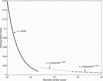
We consider a new type of constraints for modeling piecewise defined physics phenomena. Behavior laws defining complex phenomena are often established by experiments. These experiments are done under several hypotheses and conditions defining the contexts of use for these stated laws. In many cases, the main context of experiments can be managed by only one parameter, which values identify the relation to apply. For instance, many models in fluid mechanics involve the Reynolds dimensionless number. The Reynolds number values point to different types of fluid flowing (laminar, transient, turbulent) corresponding to fluid mechanics laws (see Fig. 2).
The friction factor as a function of the Reynolds number.

Let this constraint be

Such that α is a variable, each I k is an interval, and each C k is a constraint or a set of constraints. The I k identify the different cases of the piecewise phenomenon considering the parameter α and the C k correspond to the relations to use. The intersection I j ∩ Ik must be empty for every j ≠ k; otherwise, at least two constraints will apply for the same phenomenon. In other words, all the I k define a partition of the domain of α. The piecewise constraint is satisfied if

The piecewise constraint is equivalent to C k whenever α belongs to I k. At most, one k must exist because the I k do not intersect; otherwise, several constraints are taken into account, which lead to an inconsistent set of constraints.
Interval constraint satisfaction techniques are used to reduce variable domains. Let D α be the domain of α. Four cases can be identified:
1. If a k exists such that D α ⊆ I k, then C k is solved. The domains of the variables occurring in C k can be reduced using, for example, consistency techniques.
2. The domain of α can be reduced as follows:
A failure must happen if no I k intersects the domain D α.
3. If C k is violated for some k, then every element of I k can be removed from D α.
4. Otherwise, the constraint is satisfied in the interval sense but no domain can be reduced and the problem is still being underconstrained.
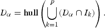
Note that the solving process must not stop before D α takes its values in at most one I k; otherwise, the piecewise phenomenon is not taken into account and many nonphysically valid solutions may be found (case 4).
2.5. Search issues
The notions of auxiliary variables and piecewise constraints introduce several difficulties and problems:
Problem 1
The splitting steps of domains for auxiliary variables may duplicate the solutions on the main variables. For same values of the main variables, several solutions for auxiliary variables may satisfy all the constraints. This is due to some incoherent precisions between auxiliary variables and main variables. It must also be highlighted that the set of auxiliary variables is often underconstrained, because, in the ED phase, some uncertainties remain about some product characteristics and its behavior. Thus, many solutions may be found for the same tuple of values for main variables. That may lead to useless redundant computations and to a huge number of approximate solutions corresponding to the same product architecture.■
Problem 2
The main variables may not be reduced enough if the auxiliary variables are not split enough. Consistency techniques used on interval domains are based on outer approximations, which may lead to an overestimation of variable domains. The solving process may be very long, spending most of the time in pure search on main variables, whereas auxiliary variables may have wide domains.■
Problem 3
It may be difficult to choose the auxiliary variables to be split and to set precision thresholds. Proper precisions are required to efficiently manage Problem 1 and Problem 2. Moreover, some auxiliary variables are only present within the model, because they define well-known properties of some components, phenomena, and so forth. However, they are not required to express all the knowledge about a product. These variables and their values improve the expressivity and comprehensibility of the product model, which is important when this model may evolve as in the ED phase. Previously, we defined them as functional variables, because their values are directly computed using an expression of other variables.■
Problem 4
The piecewise constraints must be taken into account to early reduce the search space. This clearly depends on the domain of the α variables, which must be reduced to one of the I k of the piecewise constraint to apply the constraint c k and take into account the corresponding phenomenon.■
Other Issues
ED problems are mainly underconstrained, because of the early context of this phase within the design process. We suppose here that the precisions of main variables are well chosen enough according to the domain sizes to avoid a huge number of approximate solutions. Another well-known approach is to specialize the search for integer variables and real variables.■
3. PROBLEM SOLVING
New search heuristics are introduced in this section to tackle the issues raised above. These heuristics are embedded in the general interval-based branch and prune model.
3.1. Branch and prune algorithm
The general branch and prune algorithm (Van-Hentenryck et al., Reference Van-Hentenryck, Mc Allester and Kapur1997) is defined in Algorithm 1. The input is a CSP model. The output is a set of approximate solutions enclosing the solution set.
Algorithm 1
General branch and prune algorithm.
Solve(C : set of constraints, D : domains, (x, y) : vars) : a set of interval approximate solutions
D ≔ Prune(C, D)
if D is empty then
discard D
elsif D x is precise enough then
b ≔ ProveExistence(C, D)
Insert(D x, b) in the computed approximation
else
Choose a splittable variable z in (x, y)
Split(D, z, D 1 ∪ D 2)
Solve(C, D 1, (x, y))
Solve(C, D 2, (x, y))
endif
end■
The computation is as follows. Every domain is pruned provided that no solution (element from set 1) is lost. Every approximate solution (element from set 4) associated with the result of the existence proof is inserted in the computed approximation. Nonempty domains are split, provided that at least one of the main variables is not precise enough. The subproblems are further solved.
The algorithm for the existence proof validates the box computed by the branch and prune algorithm, and several techniques may be used according to the type of constraints:
• Inequality constraints can be tackled with interval computations.
• Equality constraint systems can be processed by fixed-point operators (Kearfott, Reference Kearfott1996).
These techniques may not operate on heterogeneous and nondifferentiable problems. In this case, a search process can be used to prove the existence of canonical approximate solutions, namely, boxes of maximal precision satisfying the constraints in the interval sense. We consider that this smallest interval box, with closest floating-point numbers as bounds, is precise enough to claim that we have found a solution if no inconsistencies are detected. An other approach is to apply a local search process, where the optimization function should take into account the number of inconsistent constraints balanced by the distance of violation of each one.
However, these algorithms cannot always prove the existence of a solution within a box in reasonable time. All computed solutions may not be guaranteed, but this is not the main goal for designers to have safe numerical solutions in the ED phase. All the uncertainties relating to a model make the solutions near guaranteed boxes also acceptable. However, guaranteed boxes may correspond to more robust solutions than those for which the proof of existence has failed. In the ED phase, designers are mainly interested in having an overview of the global shape of the complete space of solutions, namely, having a better insight of the feasible product architectures. When designers have an idea of some robust solutions within a solution set, they can better define the more interesting parts of this set relating to good performances criteria and robust product architectures.
3.2. Search strategies
We propose to implement several search strategies to tackle the problems described in the previous section.
3.2.1. Splitting ratio
The choice of variables may follow an intensification process on the main variables and a diversification strategy on the auxiliary variables. The idea is to limit the duplication of solutions (Problem 1) and to compute efficient reductions on the whole system (Problem 2). A diversification process aims at gathering some knowledge on the problem, whereas an intensification process uses this knowledge to explore and to focus on interesting areas of the search space (Blum & Roli, Reference Blum and Roli2003). The intensification/diversification strategy can be controlled by a ratio between the two types of variables to choose (see Algorithm 2). Inside each group, a round-robin strategy may be used to make the algorithm robust. The round robin strategy is considered more robust for heterogeneous problems than other strategies (according to computational concerns), because variables are in equity chosen and all dimensions of the search space are explored. Other well-known strategies, like largest domain first, are not well adapted for a set composed of discrete and continuous variables, despite the fact that all domains are handled as intervals. Other strategies mainly try to exploit some characteristics of homogeneous problems. A high ratio corresponds to high intensification on main variables and a small one increases diversification on auxiliary variables.
Algorithm 2
Search heuristic favoring main variables.
SelectVariable(X : set of variables, D : domains, R : integer ratio)
X m ≔ {x ∈ X: x is a main var:, D x can be split}
X a ≔ {x ∈ X: D x can be split} \ X m
let n be the number of carried out splits
let n m be the number of splits on main var:
if X a is empty or n = 0 or n m < R(n − n m)
n m ≔ n m + 1
x ≔ SelectRoundRobin(X m)
else
x ≔ SelectRoundRobin(X a)
endif
n ≔ n + 1
return x
end■
This heuristic is applicable to any ED problem, because ED problems naturally include some main variables (where values statements are the main objective of the ED phase). Moreover, If a problem contains only main variables or auxiliary variables, then the default round-robin strategy is applied. This heuristic takes into consideration that main variables are often useful to compute relevant values for auxiliary variables. Indeed, auxiliary variables have to express some characteristics (physics phenomenon, geometry, etc.) of a specific product architecture. Main variables are better defined (small domains and accurate precisions according to the product specifications) than auxiliary variables (i.e., complex phenomena with several simplifying assumptions). In this way, the constraint propagation phase may be more interesting in reducing domains of auxiliary variables than the splitting steps on this huge search space.
3.2.2. Precision
Two types of auxiliary variables can be identified (Problem 3). Auxiliary variables expressed as functions of other variables may not be split because they correspond to intermediate computations.
To this end, it suffices to bind these variables to an infinite precision. Their values are computed using the Prune algorithm (constraint propagation). The other auxiliary variables may be split (Problem 2), but their precisions have to be as relevant as possible to avoid too many useless splitting steps (Problem 1).
3.2.3. Piecewise constraint
The goal is to split the α variable according to the first pruning case of the constraint in order to answer Problem 4. The domain of α must be included in some I k to enforce C k. To this end, the domain of α can be split on the bounds of the intervals I k instead of the classical bisection. Let us note that even the auxiliary variables with infinite precision must be considered here. Combining several piecewise constraints parametrized by the same variable comes to consider the set of bounds from all the intervals I k and to combine the constraints from the corresponding pieces.
3.2.4. Variable types
A common approach is to choose first integer variables and then real variables, supposing that different integer values may correspond to different product architectures. We then have several choice criteria to be combined: type of variable (main, auxiliary), domain nature (discrete, continuous), and more usual criteria (round-robin strategy, largest continuous domain, smallest discrete domain, most constrained variable, etc.). Integer variables are supposed to be enumerated and real variables are bisected.
3.3. Representation
Several approximate solutions are redundant if the domains of the main variables intersect, because of the search on auxiliary variables. In this case, they need to be merged to compute compact representations of the solution set. In the interval framework a set of merged boxes can be replaced by their hull, namely, the smallest box containing each element.
It must be verified that the main variables are still precise enough after merging. In particular, several boxes enclosing a continuum of solutions may share only some bounds. The hull may not be computed to keep fine-grained approximations.
4. EMPIRICAL EVALUATION ON ACADEMIC PROBLEMS
The techniques have been implemented in Realpaver (Granvilliers & Benhamou, Reference Granvilliers and Benhamou2006). The pruning step is implemented by constraint propagation using 2B consistency and box consistency. The next results do not take into account the computations of any proof of existence algorithm, because only performances of search heuristics are studied. These results are only concerned of finding solutions, which are coherent with precisions of variables. The presented curves show the number of splits made on domains of variables. Considering one solving heuristic, this number does not vary on the contrary to the solving time, which depends on the computer hardware, the operating system, and so forth. The number of splitting steps unmistakably represents the performances of each search heuristics, because the pruning algorithm is guided by it. For heterogeneous problems over large search spaces, the search heuristic plays a crucial role in the efficiency of the solving process.
4.1. Functional variables
ED problems embody many variables expressed as functions of other variables. They are maintained within the model to preserve the model intelligibility, although they could be removed and replaced by their expression. The question is whether these variables have to be split. Let us consider the following problem parametrized by n ≥ 3:
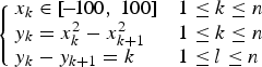
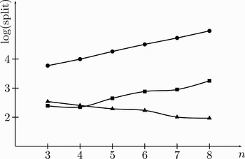
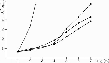
Let x n+1 be x 1 and let y n+1 be y 1. The goal is to prove that the problem has no solution. The results are depicted in Figure 3. The dotted curve corresponds to a round-robin strategy on x and no split on y. This is clearly not efficient. The square curve is obtained with a round-robin strategy on x and y. The growth ratio is almost the same (factor 2) but the number of splitting steps is decreased by a factor of 50. The triangle curve is derived by a more robust strategy such that x is split twice more than y. Surprisingly, the number of splitting steps decreases when n increases. For instance, given n = 8, the number of bisections are 93,183, 1791, and 93, respectively, for the three heuristics.
The search heuristics for functional variables. (•) A round-robin strategy on x and no split on y, (■) a round-robin strategy on x and y, and (▴) a more robust strategy such that x is split twice more than y.

Let us consider another problem parametrized by n ≥ 3:

such that x n+i = x i and y n+i = y i for every i ≥ 1. The goal is to compute the solutions on x considering a precision of 10−8 (three solutions for 6 ≤ n ≤ 11). The results are depicted in Figure 4. The dotted curve corresponds to a round robin strategy on x and no split on y. The square curve is obtained with a round robin strategy on x and y. We see that it is more efficient not to split y. The other curves are obtained with a robust strategy such that x is split r times more than y (r = 5 and 10). The improvement increases with ratio r.
The search heuristics for functional variables. (•) A round robin strategy on x and no split on y, (■) a round robin strategy on x and y, and (▴, ♦) a robust strategy such that x is split r times more than y (▴, r = 5; ♦, r = 10).

The previous results may lead to the following conclusions. In the first problem, every reduction on functional variables is directly propagated through many constraints, which is efficient because these variables occur in several constraints. If such variables appear in only one constraint, splitting them is not efficient, because they only represent intermediary computations. The second problem shows that no split on functional variables gives bad performances. In fact, every reduction on y k leads immediately to a reduction of x k+1 and x k+2 because the constraint is simple. This is a means for tackling two variables using only one split. Finally, strategies using a ratio are more robust and efficient than others on these types of problems.
It can be noted that in ED models, functional variables often take part of underconstrained network of constraints. Many splitting steps on them is useless and a high ratio is better. If this ratio is too difficult to establish, no splitting steps on functional variables is the easiest and the more efficient approach. Moreover, all splitting steps on functional variables do not have the same impact on the pruning of the whole problem and the round-robin strategy does not take this factor into account. Perhaps some other strategies, as for instance to choose the most constrained variable, should be more efficient especially with small ratios, where functional variables are often split.
4.2. Auxiliary variables
Auxiliary variables are useless from an ED point of view but they have to be efficiently managed during computations. Let us consider the following problem where n is an integer main variable in [−108, 108]; x, y, z are real variables in [−10, 10] with precision 10−8; x is a main variable; and y and z are auxiliary variables:
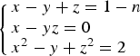
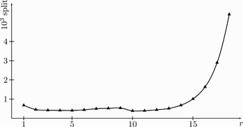
The problem projected onto the auxiliary variables is hard to solve, because this problem is dense. Local reasoning about projections may not compute efficiently variable domains. As a consequence these variables must often be split. The curve in Figure 5 is obtained from a robust strategy that alternatively splits main and auxiliary variables with ratio r. We observe an exponential behavior when r increases, that is, when auxiliary variables are seldom split. We also notice for this problem that labeling is better than bisection on n. In fact n must be set before solving the whole problem.
The search heuristics for auxiliary variables.

The number of splitting steps on auxiliary variables should follow the hardness of the problem on these variables. This theoretical criterion is not easily estimated in heterogeneous problems. It is implemented here by a global ratio on the variable sets. This ratio aims at favoring main variables according to the existential quantifier, which is defined on auxiliary variables in the context of ED problems.
4.3. Piecewise constraints
We consider the following problem:
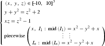
where n is the number of pieces of the piecewise constraint, each interval, and I k is defined by

where v > 0 is equal to the machine precision, and mid(I k) is the midpoint of I k. Let 10−8 be the precision of every variable.
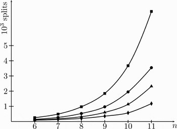
Figure 6 depicts the number of splitting steps required for solving the problem parametrized by the number of pieces of the piecewise constraint. The variables are chosen following a round robin strategy. The diamond curve is such that only the first pruning case of the piecewise constraint is applied. A restricted pruning algorithm is clearly not efficient. In this case, many approximate solutions include piece bounds, and the piecewise constraint is useless. The dotted curve corresponds to a full pruning algorithm with classical bisection, the square one to a full pruning algorithm with split on the first hole from the domain of x, and the triangle one to a full pruning algorithm with split on the mid hole. Bisection is more efficient than split on the first hole. It is known that bisection is more efficient than labeling for continuous variables. Split on the mid hole is the best heuristics. The corresponding function follows n p with 0 < p < 1. The new technique seems effective even for huge piecewise constraints.
The search heuristics for piecewise constraints. (♦) Only the first pruning case of the piecewise constraint is applied, (•) a full pruning algorithm with classical bisection, (■) a full pruning algorithm with split on the first hole from the domain of x, and (▴) a full pruning algorithm with split on the midhole.

5. EMPIRICAL EVALUATION ON REAL-WORLD PROBLEMS
In this section we evaluate our approach on models obtained for real world applications in mechanical engineering. These models take into account simplifications and assumptions inferred by the CD phase. Thus, some elements of products are frozen or neglected because this previous design phase reveals their poor significance level, while focusing on most relevant components and behaviors. This explains some unevenness within models in the appendixes. Giving all the details of the CD phase is too long, and runs over the scope of this paper. Only a brief introduction of each application is given followed by some results analysis concerning our contributions.
5.1. A basic batch exchanger system
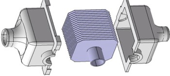
We first consider a batch exchanger model (see Fig. 7). The solution principles are defined using five design variables (three catalogs related to lengths, materials and diameters, the number of fins, and the gap between fins). In this model, the variables relating to the choices within catalogs are design variables instead of the length, materials of fins, and the diameter of the tube, which ones have their values directly defined by the catalogs. This problem is interesting from an ED point of view, because we have to choose several components in (small) catalogs while dimensioning the gap between fins. In this system, there is a coupling between fluid mechanics and the geometry of the heat exchanger (namely, the gap between fins). System modeling introduces five auxiliary variables and five functional variables. The batch exchanger is part of a batch cooler system for aperitif, and this model investigates the feasibility to cool down the aperitif from 25°C to 8°C in less than 25 s.
A batch exchanger. [A color version of this figure can be viewed online at journals.cambridge.org/aie]

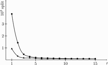
Figure 8 depicts the number of splitting steps using the robust strategy with ratio r. The number of solutions is half of the number of splitting steps. The square curve comes from labeling of integer domains and the triangle curve from bisections. We see that a high splitting ratio allows to decrease the number of splitting steps. Because of some orientation in the model the auxiliary variables are directly computed from the design variable values. Splitting auxiliary variables leads to duplicate solutions and consequently useless search steps. Bisection on integer variables is better than labeling. That is explained by efficient reductions of the number of fins (integer in [5, 20]) using some bound consistency methods.
Solving the batch exchanger problem. (■) Labeling of integer domains and (▴) from bisections.

5.2. A pump and tank water circuit
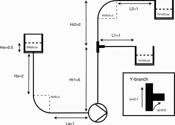
This model takes into account three tanks (one upstream and two downstream) and one water pump (see Fig. 9). The objective is to study the feasibility of dimensioning the two lines diameters after the downstream Y branch. Before the Y branch, the line diameters are 0.055 m. All the line lengths are fixed and the two downstream tanks must receive the same flow, considering that the global line sections are the same before and after the Y branch. The water pressures in the tanks are defined initially: the upstream tank is at 40,000 Pa and the two downstream tanks are open to the atmosphere air and the pressure is 101,325 Pa. The pump is standardized and has characteristics (efficiency, manometric head, required net positive suction head for a water flow, etc.) given by its manufacturer. The net positive suction head is investigated to guarantee the safety of the pump. The solutions are computed taking into account that the cavitation phenomenon in the pump must not appear; otherwise, it may be seriously damaged. The downstream circuit (directly linked to the cavitation phenomenon) is coupled to the whole circuit (pressure losses) and the Y branch make the problem nontrivial.
A pump and tank water circuit.

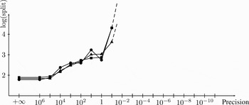
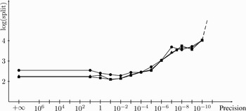
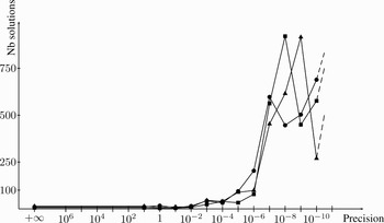
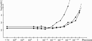
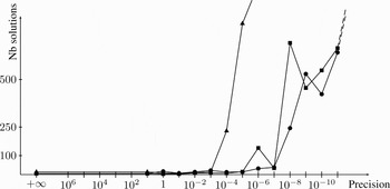
This model is made of two design variables (the two tube diameters after the Y branch), three auxiliary variables, and 35 functional variables. Figures 10–15 depict the results obtained when functional variables are split considering a global varying precision. Because the three auxiliary variables have a fixed precision, a global precision can be defined on the other variables, namely, functional variables. Thus, they are split like auxiliary variables. Half of those pictures depicts the numbers of splits and the others the number of solutions. The dotted curves show the results obtained with a classical round-robin strategy for the choices on all variables (main, auxiliary, and functional variables). The square curves express the results with a strategy always starting with main variables. Once they reach the required precision, auxiliary are variables split. The triangle curves represent the results with a choice strategy with a ratio defining a priority of three for the main variables on the auxiliary variables. Only results found within a reasonable time are written out on each curve: results with a solving time exceeding 1 h are not taken into account.
Solving the pump problem with varying precision on functional variables. (•) The worst results, in particular, for the more accurate precision, but otherwise the results are fairly similar, and (▴) the best computing run with three solutions and 296 splits for a functional variables precision of 103.

Solving the pump problem with varying precision on functional variables. (•) The worst results, in particular, for the more accurate precision, and (▴) the best computing run with three solutions and 296 splits for a functional variables precision of 103.

Solving the pump problem with several fixed and varying precisions on functional variables. (•) The worst approach, although it gives the smallest number of solutions after a precision of 10−7 for the same quantity of splits than others, and (■) the lowest number of solutions with three solutions for 148 splits for a precision of 100.

Solving the pump problem with several fixed and varying precisions on functional variables.

Solving the pump problem with more fixed precisions on functional variables and fewer ones varying than for Figures 12 and 13. (•, ▴) A maximum precision of 10−11, and (■) the best run with three solutions and 148 splits for precisions of 100 and 10−1.

Solving the pump problem with more fixed precisions on functional variables and fewer ones varying than for Figures 12 and 13.

Figures 10 and 11 represent the most general case, and all the functional variables are defined with the same global precision. The different number of solutions between each run can be explained by the miscellany of the duplication of design solutions and the powerlessness of consistency algorithms on intervals. Indeed, these algorithms have difficulties to prune accurately some domains and to reject them if they are near a solution over the real numbers. In this context, the most accurate precision on functional variables given reasonable solving time is 10−1. The dotted curve seems to have the worst results, in particular, for the more accurate precision, but otherwise the results are fairly similar. It may be noted that merging all the computed solutions gives only one design architecture. Considering that fact, the best computing run is obtained by the triangle curve with three solutions and 296 splits for a functional variables precision of 103. The best approach considering the whole curves seems to be the triangle curve, where a robust strategy is applied.
After these first results, we can observe that the precision 103 and 104 for functional variables give good results. These quantities are compatible with some functional variables values: losses in lines expressed in pascal and Reynolds number values. Thus, Figures 12 and 13 give results where these functional variables have several fixed precisions. In this case, the most accurate precision is 10−10. Globally, the dotted curve seems to be again the worst approach, although it gives the smallest number of solutions after a precision of 10−7 for the same quantity of splits than others. The lowest number of solutions is given by the square curve with three solutions for 148 splits for a precision of 100. Previously, the same small number of solutions was found, but in 296 splits.
From the maximum precision to 101 the results stay similar, but until 10−2 the number of solutions and the number of splits decrease. We can conclude that some other functional variables values are compatible with these precisions. Then, the precision of the net positive suction head, the total manometric head, and all surfaces are frozen to this last threshold. Figures 14 and 15 show the results obtained with all these precisions defined and with only a few still using the varying global precision. In this case, the robust strategy fails to give all the solutions within reasonable time after a precision of 10−8, although it seems to give the best results before a global precision of 10−3. The dotted and triangle curves allow a maximum precision of 10−11 and up to a precision of 10−7 the results are interesting. The best run is obtained by the square curve with three solutions and 148 splits for precisions of 100 and 10−1, which is not better than in the previous case.
With these results, we can conclude that some of the functional variables have to be split (using CSP based on interval arithmetic). But it is difficult to define a relevant precision on each functional variable, because some of them are only intermediary computations, which are difficult to measure before the solving process. Functional variables that can be split must have a precision relating to the magnitude of their consistent values and relating to the confidence awarded to the corresponding constraints. Otherwise, a large precision inducing few splits is better not to increase the search space and to dramatically duplicate solutions.
5.3. A bootstrap problem
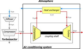
A basic model of an aircraft air conditioning system is investigated (see Fig. 16). Air coming from a turboreactor and from the atmosphere is used to produce suitable air for the crew. The atmosphere air cools down the air coming from the turboreactor through a heat exchanger where complex piecewise defined physics phenomena are studied (Fanning friction factor and Nusselt number). The turboreactor air flow passes through a compressor to improve the heat transfer phenomenon inside the exchanger. Before exiting the air conditioning system, a turbine releases its pressure and makes its temperature decrease. A coupling shaft conveys to the compressor the mechanical energy produced by the turbine. This problem is difficult to solve because many physics phenomena interfere. The loop corresponding to the bootstrap make its components coupled according to the temperatures and pressures of the air flux. These temperatures and pressures are also linked to the heat exchanger geometry (gap between plates).
The bootstrap flux flow diagram in an aircraft. [A color version of this figure can be viewed online at journals.cambridge.org/aie]

In this model, the compressor, the turbine and the coupling shaft are standardized components, and only the heat exchanger has to be embodied as it mainly determines the air-conditioning performances. The main objective of the system is to bring air to the passengers and the crew of the aircraft and to control the air temperature and pressure inside the cockpit. But some other criteria are important in an aircraft, as the air flow taken from the turboreactor (that decreases its efficiency), the increase of the aircraft drag, the weight of the air-conditioning system, and so forth. This problem is efficiently solved with piecewise constraints: 6734 splitting steps and 1262 approximate solutions with respect to 36,978 splitting steps and 18,860 approximate solutions without piecewise constraints.
Moreover, this problem cannot be solved within reasonable time with classical round-robin strategies on all the variables. The search space is so wide that if the ED knowledge about main variables is not used, the solving process becomes very long. The use of functional variables with infinite precision is the easiest way, because the model is complex. Moreover, quantities represented by functional variable values can vary, as for instance the Reynolds number, which takes its values from 100 to 200,000.
It may be noted in the solution set of these real problems, that auxiliary variables precision are sometimes large. Indeed, the interval computations compute interval solutions, which is an approximation of at least one solution over the real numbers. If the model is very sensitive to main variables values and if their precisions are not small enough, auxiliary variables may have large domains, which contain several consistent values. In the context of ED, the main goal for designers is to investigate the feasibility of design concepts. Their first interest is to know where there is no solution in the search space. If they really want to have more precise auxiliary variable values for one specific design architecture, they just have to change all variables domains corresponding to one or several computing solution values and then to increase variable precisions. They can start a new solving phase on this more restricted search space and find more accurate numerical solutions.
6. RELATED WORK
Constraint techniques may be used at two successive stages of preliminary design. Discrete constraints may lead to determine the architecture of a product during the CD phase (O'Sullivan, Reference O'Sullivan2001). CD using components from the shelf is known as configuration. These problems can be represented by dynamic constraint satisfaction problems (Mittal & Falkenhainer, Reference Mittal and Falkenhainer1990) such that the involved components are activated and the corresponding constraints are solved. The notion of component (or variable) activation can be tackled by conditional constraints (Gelle & Faltings, 2003; Sabin et al., Reference Sabin, Freuder and Wallace2003). Larger and more complex problems are also tackled by Mailharro (Reference Mailharro1998) and Stumptner et al. (Reference Stumptner, Friedrich and Haselböck1998). From a solving point of view the main goal is to efficiently traverse the tree of architectures. Numerical nonlinear constraints are more involved in the ED phase. The frontier between CD and ED may be thin because mixed constraints can be considered (Gelle & Faltings, Reference Gelle and Faltings2003) to tackle both phases at the same time. But However, the ED physics models are in general more complex.
Sam-Haroud and Faltings (Reference Sam-Haroud and Faltings1996) have proposed to represent numerical constraints by 2k-trees, namely, decompositions of the feasible regions using interval boxes. Strong consistency techniques have been defined through the combination of 2k-trees. Design applications such as bridge design have been efficiently solved. In this framework, constraint systems are decomposed in binary and ternary constraints in order to limit the size of 2k-trees (quadtrees if k = 2 and octrees if k = 3).
Classical interval techniques have been implemented in the ED platform Constraint Explorer (Zimmer & Zablit, Reference Zimmer and Zablit2001). The solving engine combines interval arithmetic, constraint propagation, and search. An important feature is the analysis of the constraint network using graph decomposition (Bliek et al., Reference Bliek, Neveu and Trombettoni1998). The result of this analysis is an ordering of variables to be fixed before solving the associated constraint blocks. Recent developments can be found in (Neveu et al., (Reference Neveu, Chabert and Trombettoni2006). Our approach can be directly integrated for solving one block. In particular, large blocks may arise in ED models, for instance, in the study of the equilibrium of a system.
Piecewise constraints can be implemented by means of conditional constraints (Zimmer & Zablit, Reference Zimmer and Zablit2001). This method amounts to the first case of our pruning algorithm. More recently, binary piecewise constraints with pieces in the form of (x, y) ∈ Ik × Jk : C k(x, y) have been represented by quadtrees (Vareilles et al., Reference Vareilles, Aldanondo, Gaborit and Hadj-Hamou2005). It seems difficult to extend this approach to constraints of higher arities, which is required for solving the problems described in this paper.
Solution sets with nonzero volumes may be characterized by inner approximations, namely, interval boxes of which every point is a solution. Several works have tackled specific cases: inequality constraints by means of 2k-trees (Sam-Haroud & Faltings, Reference Sam-Haroud and Faltings1996), interval boxes (Collavizza et al., Reference Collavizza, Delobel and Rueher1999), or the extreme vertex representation (Vu et al., 2002), and equality constraint systems with at least as many existential quantifiers as equations (Goldsztejn & Jaulin, Reference Goldsztejn and Jaulin2006). The study of such techniques for more heterogeneous constraint systems is an issue.
Other works have taken into account relations that are not described by analytical expressions (Yannou et al., Reference Yannou, Simpson and Barton2003; Fischer et al., Reference Fischer, Sébastian, Nadeau and Zimmer2004), exploiting in the constraint framework simulation results or data from black box numerical tools. The main idea is to compute approximate constraint-based models of these relations.
7. CONCLUSION
ED problems have been represented by constraint satisfaction problems with existential quantifiers. ED knowledge concerning types of variables and their precision has been used to improve the solving efficiency. New search heuristics based on a splitting ratio have been introduced to tackle the quantified variables. Duplicated solutions of main variables are drastically reduced, and decisions concerning the design solution principles are easier to make for designers. A global constraint has been defined for piecewise defined physics phenomena. Experimental results from academic and real-world problems are promising. ED goals are better taken into account because the main purpose is to investigate the feasibility of the search space while getting a set of approximated solution principles covering the whole solution principles.
There are many directions for future research. The notion of splitting ratio could be refined to tackle the hardness of every variable. The hardness of a variable should be clearly defined. For instance, dependencies between variables may also indicate variables relevance in the model and surely participate to evaluate their hardness. Auxiliary variables precision and the validation of solutions could be more studied. The notion of precision is essential in numerical computations. The precision on auxiliary variables is not often chosen appropriately, and it induces many useless computations steps in all search heuristics. Precision of main variables is easily defined considering the design knowledge about the model (i.e., epistemic knowledge about main variable values). In contrast, auxiliary variables are often part of complex mathematical expressions. In fact, the sensitivity of each variable should be investigated, and precision should be defined considering the numerical analysis of each constraint in which variables are involved. Nevertheless, in practice, it is very difficult to apply over heterogeneous problems, and designers have no time to investigate in those fastidious calculations. The solving process has to be fast because designers do not want to perform complete simulations of a product. Moreover, the integration of our techniques in a block solving approach could be explored. The block decomposition of a CSP takes into account the constraints network and allows the establishing of an order or a causality on variables or blocks of variables. In most design models, starting variables are needed to compute a relevant order, because models are often underconstrained. Several orders on variables may be defined for the same constraint graph, and the choice of the optimal one is undecidable within reasonable time (Jégou & Terrioux, Reference Jégou and Terrioux2003), but our heuristic favoring main variables may help in this ordering task, while taking into account design knowledge.
R. Chenouard holds a teaching position in computer science at the University of Nantes. He received his PhD at the Arts et Métiers Paristech in Bordeaux, where he was awarded the 2008 Bezier Prize. Dr. Chenouard investigates embodiment design models with constraint programming techniques over discrete and continuous domains. His current research includes model-driven approaches to handle models and several numerical solving methods to better process these models.
L. Granvilliers is a Professor of computer science at the University of Nantes, where he is the leader of the MEO research team. He is the President of the University Employment Commission in Computer Science, the founder and former director of the MSc of Software Architectures, and Professor in charge of the second year of the international master's of science in optimization in operations research. His current research includes global optimization, constraint programming, interval analysis, modeling languages, and optimization systems.
P. Sébastian is an Associate Professor of energy and process engineering at the University of Bordeaux 1. He is a member of the Scientific Advisory Board of the International Conference on Virtual Concept. His current research includes embodiment design of complex mechanical systems using, for instance, adaptation methods to improve decision support provided by models at this early design stage.
APPENDIX A: Batch-exchanger model
Constant names and values

Design variable names, domains, and precisions

Auxiliary variable names and domains

Functional variable names and definition

Constraints

APPENDIX B: Pump and tank water circuit model
Constant names and values

Design variable names, domains, and precisions

Auxiliary variable names and domains

Functional variable names and definition

Constraints

APPENDIX C: Bootstrap model
Constant names and values

Design variable names, domains, and precisions

Auxiliary variable names and domains

Functional variable names and definition

Constraints