2. Numerical methods

The trajectories of inertial particles used in this work were obtained by numerically integrating the equation of motion

(2.1) \begin{align}&\quad \frac {{\textrm d} \mathbf{x}}{{\textrm d} t} = \mathbf{v}, \\[-12pt] \nonumber \end{align}

(2.2) \begin{align}& \frac {{\textrm d} \mathbf{v}}{{\textrm d} t} = \frac {\mathbf{u} - \mathbf{v}}{\tau _p}, \end{align}

where $\mathbf{x}$ and $\mathbf{v}$ are the particle position and velocity, respectively, $\mathbf{u}$ is the fluid velocity at the particle position, which was interpolated from a forced homogeneous isotropic turbulent flow at a Taylor microscale-based Reynolds number $R_{\lambda } = 433$ maintained in the Johns Hopkins Turbulence Database (Li et al. Reference Li, Perlman, Wan, Yang, Meneveau, Burns, Chen, Szalay and Eyink2008), and $\tau _p$ is the particle relaxation time. In this work, we studied 4 different inertial particles with $St \equiv \tau _p/\tau _\eta = 0.3$ , $0.5$ , $0.7$ and $1$ , for which the caustic effects are expected to be significant. For each Stokes number, the inertial particles were released in 125 groups with the initial positions of group centres on a $5 \times 5 \times 5$ grid distributed uniformly in the simulation domain of size $(2\pi )^3$ . In each group, there were $15 \times 15 \times 15$ particles initially arranged on a grid with a uniform spacing of $0.5 \eta$ and initialised with fluid velocities at their initial positions. Initially, the $15 \times 15 \times 15$ particles in a group were arranged on a regular cubic grid with grid spacing of $0.5 \eta$ . Thus, the $15 \times 15 \times 15$ particles in a group were uniformly distributed in a cube of size $(7\eta )^3$ in the flow field. There were in total $5 \times 5 \times 5 = 125$ such groups and initially the geometric centres of these groups were distributed uniformly in the simulation domain of size $(2\pi )^3$ , i.e. the distance between neighbouring group centres was $2\pi /5 \approx 400\eta$ .

The equation of motion was integrated using the third-order Adams–Bashforth method (Chang, Malec & Shaw Reference Chang, Malec and Shaw2015) with the first two time steps started by the fourth-order Runge–Kutta method. The time steps were $\Delta t = \tau _p/20$ and the total times of integration were $90 \tau _p$ , but the statistics used in this work started from $20 \tau _p$ to avoid the initial transient period (Chang et al. Reference Chang, Malec and Shaw2015). Overall, for each $St$ , we collected trajectories of $(15^3) \times (5^3) = 4\,21\,875$ inertial particles, each lasted for a time of $70 \tau _p$ . For each particle trajectory, the instantaneous fluid velocities at the particle positions were also recorded for later analyses. The particles were then transported by the fluid and dispersed in the flow field. We collected statistics of the particles $20\tau _p$ after their release, at which point the particle accelerations had already reached a statistically steady state, as shown in figure 1. Note that, in figure 1, the particle acceleration magnitudes were normalised by the root-mean-square value of the fluid acceleration $\langle a^2\rangle ^{1/2}$ , which was calculated from turbulence energy dissipation rate of the flow $\langle \epsilon \rangle$ using the Heisenberg–Yaglom scaling (Heisenberg Reference Heisenberg1948; Yaglom Reference Yaglom1949)

(2.3) \begin{equation} \langle a_i a_j \rangle = a_0 \langle \epsilon \rangle ^{3/2} / \nu ^{1/2}, \end{equation}

which has been examined by many experimental measurements and DNSs and the dimensionless constant $a_0$ is found to be around $6$ for high Reynolds number turbulence (La Porta et al. Reference La Porta, Voth, Crawford, Alexander and Bodenschatz2001). In addition to particle acceleration, we also checked other statistics shown later and verified that they remained unchanged with the time period over which the statistics were calculated.

Figure 1.

The average acceleration magnitude of inertial particles with the time since their release in the fully developed turbulence field. The vertical dashed line indicates the time after which the statistics shown in the manuscript were collected.

If the particle velocity field is well behaved, by taking the spatial gradient of (2.2), we obtain the evolution equation of the particle velocity gradient $M_{ij} = \partial v_i / \partial x_j$ as

(2.4) \begin{equation} \frac {\textrm d M_{ij}}{{\textrm d}t} = \frac {A_{ij}-M_{ij}}{\tau _p} - M_{ij}M_{ji}, \end{equation}

in which $A_{ij} = \partial u_i / \partial x_j$ is the fluid velocity gradient. In previous investigations, (2.4) is integrated directly along the particle trajectory together with solving the velocity field by DNS to study the dynamics of $M_{ij}$ (see, e.g. Falkovich et al. (Reference Falkovich, Fouxon and Stepanov2002); Wilkinson & Mehlig (Reference Wilkinson and Mehlig2005); Falkovich & Pumir (Reference Falkovich and Pumir2007)). The major limitation of this approach is that, at caustics, the particle velocity gradient $M_{ij}$ becomes singular and (2.4) is not valid any more. Thus, while this approach can be used to study the dynamics of inertial particles before caustics, it is difficult to be applied to post-caustics. This limitation is what we aim to overcome in this work. Furthermore, note that, at the moment when a caustic happens, the particle velocity field is obviously not well behaved, the particle velocity gradient cannot be defined and (2.4) is not valid. On the other hand, in our numerical simulations and the subsequent analyses of the particle velocity gradient, we do not need the assumption of a well-behaved particle velocity field. Our approach is to use the data of discrete particles to obtain its velocity gradient, as shown below.

To obtain $M_{ij}$ from the particle trajectories, we notice that the perceived velocity gradient from the tetrad model (Chertkov et al. Reference Chertkov, Pumir and Shraiman1999) is an efficient tool to study the Lagrangian dynamics of fluid turbulence from the trajectories of 4 fluid tracers, e.g. the interaction between the local straining and rotation along fluid elements (Xu et al. Reference Xu, Pumir and Bodenschatz2011; Pumir et al. Reference Pumir, Bodenschatz and Xu2013; Yang, Pumir & Xu Reference Yang, Pumir and Xu2020). In particular, it has been shown that, when the distances between the 4 fluid tracers are within the Kolmogorov length scale $\eta$ , the perceived velocity gradient recovers faithfully the true fluid velocity gradient (Pumir et al. Reference Pumir, Bodenschatz and Xu2013). Motivated by this, here, we define the particle velocity gradient $\mathbf{M}$ based on a group of $N$ particles within a small neighbourhood relative to their centre of mass, i.e. $\forall \alpha \in [1,N]$ , $\vert \mathbf{X}^{\alpha } \vert = \vert \mathbf{x}^{\alpha } - \mathbf{x}^{0} \vert \lesssim \eta$ , where $\mathbf{x}^0 = ({1}/{N}) \sum _{\alpha = 1}^{N} \mathbf{x}^\alpha$ is the centre of mass of the group. The relative velocity of the particle with respect to their centre of mass is $\mathbf{V}^{\alpha } = \mathbf{v}^{\alpha } - \mathbf{v}^{0}$ , with $\mathbf{v}^0 = ({1}/{N}) \sum _{\alpha = 1}^{N} \mathbf{v}^{\alpha }$ . Then, $\mathbf{M}$ is the local velocity gradient that best fits all the relative velocities in the least square sense

(2.5) \begin{equation} M_{ij} \equiv g^{-1}_{ik}\sum _{\alpha =1}^{N} X_{k}^{\alpha } V_{j}^{\alpha }, \end{equation}

with

(2.6) \begin{equation} g_{ij} \equiv \sum _{\alpha =1}^{N} X_{i}^{\alpha } X_{j}^{\alpha } \end{equation}

being a tensor that describes the size and geometry of the structure formed by the group of particles. To efficiently choose the particles within a small region, we employ the ‘cell-box’ method (Quentrec & Brot Reference Quentrec and Brot1975; Sundaram & Collins Reference Sundaram and Collins1997) by dividing the simulation domain into small cubic cells with side length of $\eta$ and count the particles within the same cell. It is clear that to uniquely define $\mathbf{M}$ in three-dimensional space, we need $N \geqslant 4$ . On the other hand, for $N=4$ , when the 4 particles are on the same plane, the matrix $\mathbf{g}$ is singular and cannot be inverted to define $\mathbf{M}$ . Even when the 4 particles are not co-planar, but very close to, the inversion of $\mathbf{g}$ is mathematically difficult. Therefore, to reduce this difficulty, we require in this work that $N \geqslant 5$ , which is important as caustics feature significant flattening of the particle group in the largest compression direction (Bätge et al. Reference Bätge, Fouxon and Wilczek2023), as will be reported below from our analyses.

Similar to the definition of the particle velocity gradient $\mathbf{M}$ , when studying the evolution of $\mathbf{M}$ described by (2.4), we define the fluid velocity gradient $\mathbf{A}$ as

(2.7) \begin{equation} A_{ij} \equiv g^{-1}_{ik}\sum _{\alpha =1}^{N} X_{k}^{\alpha } U_{j}^{\alpha }, \end{equation}

in which $\mathbf{U}^{\alpha } = \mathbf{u}^{\alpha } - \mathbf{u}^{0}$ , with $\mathbf{u}^0 = ({1}/{N}) \sum _{\alpha = 1}^{N} \mathbf{u}^{\alpha }$ , and $\mathbf{u}^{\alpha } = \mathbf{u}(\mathbf{x}^{\alpha })$ is the fluid velocity at the particle position. This definition ensures that the fluid dynamics experienced by the discrete particles is accurately captured.

3. Single-time statistics of inertial particles

From the data collected, we first ask whether at any instantaneous time the inertial particles prefer some special turbulence structure. To that end, we represent the local flow structure by the non-trivial invariants of the fluid velocity gradient $\mathbf{A}$ where the particle is located, i.e. $Q \equiv -\textrm { tr}(\mathbf{A}^2)/2$ and $R = -\textrm { tr}(\mathbf{A}^3)/3$ (Vieillefosse Reference Vieillefosse1982, Reference Vieillefosse1984; Chong, Perry & Cantwell Reference Chong, Perry and Cantwell1990). Figure 2(a) shows the joint probability density function (JPDF) of $R$ and $Q$ at the positions of tracer particles, i.e. $P(R,Q|St=0)$ , which is the familiar ‘tear-drop’ shape for fluid tracers observed before in many turbulent flows (Soria et al. Reference Soria, Sondergaard, Cantwell, Chong and Perry1994; Blackburn, Mansour & Cantwell Reference Blackburn, Mansour and Cantwell1996; Ooi et al. Reference Ooi, Martin, Soria and Chong1999). Figure 2(b) shows the JPDF of $R$ and $Q$ at the positions of inertial particles with $St =1$ , $P(R,Q|St=1)$ , which, from the first look, is very similar to the JPDF for fluid tracers. To see the effect of inertia on the distribution of particles in turbulence, we plot the ratio of the JPDF for inertial particles to that of the fluid tracers, which was obtained by sampling $\mathbf{A}$ uniformly in space. As shown in figures 2(c)–2(f), inertial particles are more likely to lie in the region with $R\gt 0$ and $Q\lt 0$ , and below the so-called Vieillefosse tail, which corresponds locally to two stretching directions and one compression direction and is also known as the ‘colliding jet’ (Betchov Reference Betchov1956) or ‘unstable saddle node’ (Chong et al. Reference Chong, Perry and Cantwell1990) local flow structure. This result is consistent with Perrin & Jonker (Reference Perrin and Jonker2016), who reported that inertial particles tend to accumulate in unstable saddle nodes of the turbulent flow in their DNS.

We note that, by taking the trace of (2.4) and neglecting terms of order $O(St^2)$ and higher, one obtains $\nabla \cdot \mathbf{v} \approx 2 St Q$ , which shows the preferential concentration that inertial particles prefer $Q\lt 0$ or strain-dominating regions (Maxey Reference Maxey1987; Wang & Maxey Reference Wang and Maxey1993). The results shown in figure 2 clarify further where inertial particles accumulate.

To calculate those JPDFs, we divided the range of interest, $\tau _{\eta }^2 Q \in [-5,5]$ and $\tau _{\eta }^3 R \in [-5,5]$ , into $200$ intervals in each direction, which forms $200 \times 200$ bins on the $(R,Q)$ plane. We then counted the number of samples in these bins, from which the probability of falling in each bin can be obtained. The JPDF was then calculated by dividing the counts by the bin area $\Delta R \times \Delta Q$ . The statistical convergence can be judged by noticing that for a bin with a PDF value of the order of $10^{-3}$ , it contains approximately $10^4$ samples.

Figure 2.

(a) Shows $P(R,Q|St=0)$ , the JPDF of $R$ and $Q$ on the position of tracer particles with $St=0$ ; (b) $P(R,Q|St=1)$ , the JPDF of $R$ and $Q$ on the position of inertial particles with $St=1$ ; (c)–(f) ${P(R, Q|St\gt 0)}/{P(R, Q|St=0)}$ , the ratio of $P(R, Q|St)$ for inertial particles with $St=0.3 \sim 1$ and fluid tracers. In each panel, the white dashed line represents the Vieillefosse tail and the white solid line represents ${P(R, Q|St\gt 0)}/{P(R, Q|St=0)}=1$ .

For particles with smaller Stokes numbers, the region with $P(R, Q|St\gt 0) \gt P(R, Q|St=0)$ extends to a more elongated shape along the Vieillefosse tail. With the increase of $St$ , this region shrinks towards $(R,Q) = (0,0)$ . This suggests that, although inertial particles tend to cluster in compression-dominated regions of the flow field, particles with higher inertia are less likely to appear in regions with intense compression.

Figure 3.

(a)–(d) The JPDF of the longitudinal component of $\mathbf{M}$ and $\mathbf{A}$ , $P(M_{11}, A_{11})$ , for different $St$ ; (e)–(h) the JPDF of the smallest eigenvalue of $(\mathbf{M}+\mathbf{M}^T)/2$ , $\lambda _3^P$ , and the rate of strain of $\mathbf{A}$ projected in the corresponding direction, $S_{33}$ . The red rectangular boxes marks the branches that indicate the post-caustic events.

In isotropic turbulence, the dynamics of the particle velocity gradient $\mathbf{M}$ could be partially probed through the interaction between the longitudinal components of $\mathbf{M}$ and the fluid velocity gradient $\mathbf{A}$ . In figures 3(a)–3(d), we plot, for particles with different $St$ , the JPDF of $M_{11}$ and $A_{11}$ , which are the straining rates in the $x_1$ direction from the data and equal the straining rate in any specific direction in an isotropic flow. In the limit of $St \to 0$ , we expect the PDF to concentrate along the diagonal as $\mathbf{M} \approx \mathbf{A}$ , which is approximately the case for $St = 0.3$ but with noticeable deviation in the region $A_{11} \lt 0$ below the diagonal, which means that stronger compression in the particle phase occurs in regions with fluid compression, i.e. the formation process of caustics. These events are also what Bewley et al. (Reference Bewley, Saw and Bodenschatz2016) focused on in their experiments. With the increase of $St$ , this signature of caustic formation is more pronounced. On the other hand, it is interesting to note that, for higher $St$ , the JPDF also branches along the direction $A_{11} \lesssim 0$ while $M_{11} \gt 0$ , which means that particles are separating from each other in the direction where the fluid is compressing. This corresponds to the post-caustic events where particles with large enough inertia penetrate through the fluid motion and move apart. Defining $\mathbf{M}$ from particle trajectories allows us to explore this process that is not accessible in the continuum description.

In figures 3(e)–3(h), we plot the JPDFs of $\lambda _3^P$ and $S_{33}$ , where $\lambda _3^P$ is the smallest eigenvalue of the symmetric part of $\mathbf{M}$ , i.e. the rate of the most compression in the particle phase, which dominates the dynamics of caustic formation (Bätge et al. Reference Bätge, Fouxon and Wilczek2023), and $S_{33} \equiv {\hat{\mathbf{e}}}^P_3 \cdot \mathbf{S} \cdot {\hat{\mathbf{e}}}^P_3$ is the straining rate of the fluid in that direction, with ${\hat{\mathbf{e}}}^P_3$ being the eigenvector of $\mathbf{M}$ corresponding to $\lambda _3^P$ and $\mathbf{S} = (\mathbf{A}+\mathbf{A}^T)/2$ being the symmetric part of  $\mathbf{A}$ . These plots show clearly that, compared with $M_{11}$ , there is a much higher probability for $\lambda _3^P$ to develop negative values with $\lambda _3^P \ll S_{33}$ , i.e. particles approaching each other at a rate much faster than the fluid, indicating the caustic events (Falkovich et al. Reference Falkovich, Fouxon and Stepanov2002; Wilkinson & Mehlig Reference Wilkinson and Mehlig2005; Gustavsson & Mehlig Reference Gustavsson and Mehlig2013; Bätge et al. Reference Bätge, Fouxon and Wilczek2023). As $St$ increases from 0.3 to 1, the peak of negative values of $\lambda _3^P \ll S_{33}$ occurs at $S_{33}$ with smaller magnitude, which suggests that, for particles with higher $St$ , caustics can be triggered by weaker fluid compression.

4. Formation process of the caustic events

The statistics shown above reveal an interesting relation between $\mathbf{M}$ and $\mathbf{A}$ at a single time. On the other hand, the caustic formation process is better studied in a Lagrangian view, i.e. following a group of particles that experiences a caustic event. To that end, we first identify those groups by searching for the events when $\textrm {tr}(\mathbf{M}) \leqslant C$ with a threshold $C \lt 0$ . We tested several choices of the threshold and found that, when $C \approx -1/\tau _p$ , which has also been commonly used before to define caustics (Falkovich & Pumir Reference Falkovich and Pumir2007; Bewley et al. Reference Bewley, Saw and Bodenschatz2016; Meibohm et al. Reference Meibohm, Gustavsson and Mehlig2023), the results presented below depend very weakly on the exact threshold value. We then follow that group of particles before and after the time when $\textrm {tr}\mathbf{M} \leqslant C$ . In this way, we obtain an ensemble of particle group trajectories that experience strong compression events, and we also compute the particle and fluid velocity gradients $\mathbf{M}$ and $\mathbf{A}$ along the trajectories. During the time investigated the average inter-particle distance is always $\sim \eta$ , but the individual inter-particle distance might be large at some times, at which $\mathbf{M}$ and $\mathbf{A}$ should be considered as the perceived velocity gradients at larger scales (Xu, Ouellette & Bodenschatz Reference Xu, Ouellette and Bodenschatz2008; Pumir et al. Reference Pumir, Bodenschatz and Xu2013).

Figure 4.

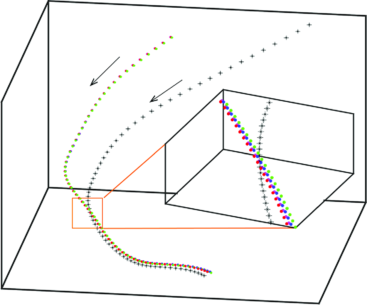
A sketch of the caustic process experienced by a group of inertial particles in turbulence seen at three sequential times $t_{1} \lt t_{2} \lt t_{3}$ . The solid arrows represent the background fluid flow field and the dashed lines represent the trajectories of inertial particles, which are represented by the spheres. The colours are used only to mark where the particles start. Due to their inertia, the particles can penetrate through the separatrix in the fluid flow field. During the process, the structure formed by the inertial particles may become nearly co-planar, corresponding to a vanishingly small value for the smallest eigenvalue of the $g_{ij}$ matrix, which is what we defined as the formation of caustics and used as the reference time, i.e. for this event, we set $t= 0$ at time $t_{2}$ .

To obtain the Lagrangian statistics from the ensemble, we also need to define the time corresponding to ‘the instant of caustics’, which we choose to be the time when the particle group collapses to a nearly co-planar configuration, which can be measured from the relative magnitude of the smallest eigenvalue of the shape tensor $\mathbf{g}$ defined by (2.6) (Xu et al. Reference Xu, Ouellette and Bodenschatz2008; Pumir et al. Reference Pumir, Bodenschatz and Xu2013). It is easy to see that $\mathbf{M}$ blows up when the structure tensor $\mathbf{g}$ is not invertible, or when its smallest eigenvalue becomes zero (note that $\mathbf{g}$ is positive semi-definite). Geometrically, this means that the group of particles are co-planar. When processing real data, a group of more than 3 particles can never be exactly on the same plane, that is, the smallest eigenvalue of $\mathbf{g}$ can never be exactly zero, but very small, which makes the value of $\mathbf{M}$ computed from (2.5) extremely large, which is in fact the manifestation of the singularity or the caustic event by discrete particles, as shown by the sketch in figure 4. For each group, we choose $t=0$ to be when $\lambda _3^g$ $({\lambda _1^g+\lambda _2^g+\lambda _3^g})$ reaches a small threshold $10^{-3}$ , where $\lambda _1^g \gt \lambda _2^g \gt \lambda _3^g$ are the eigenvalues of $\mathbf{g}$ . We have tested and seen that the results does not depend sensitively on the exact value of the threshold chose. We then collect statistics by aligning the time at $t=0$ and denote the averages over particle groups by $\langle \cdot \rangle$ .

Figure 5.

Panels (a) and (b) show the eigenvalues of $\mathbf{S}$ , normalised by $\tau _\eta$ and $\tau _p$ , respectively, along the trajectories of particles experiencing caustic events. (c) The averaged paths of $\mathbf{A}$ on the $(R,Q)$ plane before caustics, where the solid dots represent the extreme of $(\langle R\rangle , -\langle Q\rangle )$ along each path and the black arrows represent the direction of time. The inset shows the change of the normalised maximum values $\tau _p^3\langle R\rangle _{{ max}}$ and $-\tau _p^2 \langle Q\rangle _{{ max}}$ with $St$ . In all plots, $\times$ , $\triangledown$ , $\circ$ and $\square$ symbols represent $St = 0.3$ , $0.5$ , $0.7$ and $1.0$ , respectively.

To see how the fluid velocity gradient $\mathbf{A}$ experienced by the particles evolves, figure 5(a) shows $\langle \lambda _i^F \rangle$ , the averaged eigenvalues of $\mathbf{S} = ({1}/{2})(\mathbf{A} + \mathbf{A}^T)$ along the particle trajectories, with $\lambda _1^F \gt \lambda _2^F \gt \lambda _3^F$ . As stated earlier, at $t=0$ the group of particles is very close to being co-planar and it is difficult to measure the three-dimensional velocity gradients $\mathbf{M}$ and $\mathbf{A}$ from the inversion of $\mathbf{g}$ . Thus, we did not include the results near $t=0$ . In figure 5(a), the sign of the intermediate eigenvalue is $\langle \lambda _2^F \rangle \gtrsim 0$ , which confirms that caustics tend to occur in regions with the local flow structure corresponding to ‘jet collision’ (Betchov Reference Betchov1956) or an unstable saddle node (Perrin & Jonker Reference Perrin and Jonker2016). Furthermore, $\langle \lambda _{3}^{F} \rangle$ reaches a minimum in $t\lt 0$ , indicating that the strongest fluid compression was experienced before the caustic event (Bätge et al. Reference Bätge, Fouxon and Wilczek2023; Meibohm et al. Reference Meibohm, Gustavsson and Mehlig2023). With the increase of $St$ , the magnitude of the minimum of $\langle \lambda _{3}^{F} \rangle$ , when normalised by $\tau _\eta$ , decreases, which suggests that particles with smaller inertia must be subject to stronger fluid compression for the formation of caustics, making them less prone to form caustics. The argument above suggests that $\tau _p$ might be the proper time scale to normalise $\langle \lambda _{3}^{F} \rangle$ . Figure 5(b), however, shows that $\tau _p \langle \lambda _{3}^{F} \rangle$ cannot collapse the statistics with different $St$ either.

Figure 5(c) projects the evolution of $\mathbf{A}$ during caustic formation on the ( $R,Q$ ) plane. Note that the result of $\langle \lambda _2^F \rangle \gtrsim 0$ implies that $\langle R \rangle \gt 0$ because $R = - \lambda _1^F \lambda _2^F \lambda _3^F$ and $\lambda _1^F \gt 0$ and $\lambda _3^F \lt 0$ . In addition, figure 3 and the argument leading to preferential concentration suggests that inertial particles accumulate in regions with $Q \lt 0$ . Thus we expect the paths of the caustic formation process to lie in the quadrant of $R\gt 0$ and $Q\lt 0$ on the ( $R,Q$ ) plane. Figure 5(c) confirms this. Moreover, for all $St$ , the averaged paths cluster just below the Vieillefosse tail, indicating a preference for caustic events to occur in compression-dominated regions. For each $St$ , in accordance with the increase of the magnitude of $\langle \lambda _3^F \rangle$ , the path progresses along the Vieillefosse tail towards the right until it reaches a maximum in $(R, -Q)$ , signifying the occurrence of the strongest local fluid compression. The paths then revert towards the origin before the caustic event. This is qualitatively consistent with the results obtained in a recent study using a Gaussian model for the fluid velocity field, which shows that inertial particles with $St \lesssim 0.3$ experience a threshold value $Q(St)$ before caustics (Meibohm et al. Reference Meibohm, Gustavsson and Mehlig2023).

As $St$ decreases, i.e. for particles with smaller inertia, the maximum of $(R, -Q)$ experienced by the particles, when normalised by $\tau _\eta$ , extends further towards the right. The inset of figure 5(c) shows that, when normalised by $\tau _p$ , these maximum values, $\tau _p^3 \langle R \rangle _{{ max}}$ and $-\tau _p^2\langle Q \rangle _{{ max}}$ , grow linearly with $St$ , implying that $\langle R \rangle _{{ max}} \sim (\tau _p^2 \tau _\eta )^{-1}$ and $-\langle Q \rangle _{{ max}} \sim (\tau _p \tau _\eta )^{-1}$ . Thus the results shown in figure 5 suggest that the dynamics of caustic formation is not simply determined by either $\tau _p$ or $\tau _\eta$ alone.

Figure 6.

(a) Evolution of $\langle \lambda _3^P(t\lt 0) \rangle$ (magenta) and $\langle S_{33}(t\lt 0)\rangle$ (red) before caustics followed by $\langle \lambda _1^P (t\gt 0)\rangle$ (dark green) and $\langle S_{11} (t\gt 0) \rangle$ (blue) after caustics. The inset shows the alignment of the eigenvalues $\langle [{\hat{\mathbf{e}}}^P_3(t=-0.3\tau _\eta ) \cdot {\hat{\mathbf{e}}}^P_1(t)]^2 \rangle$ (cyan) and $\langle [{\hat{\mathbf{e}}}^F_3(t=-0.3\tau _\eta ) \cdot {\hat{\mathbf{e}}}^F_1(t)]^2 \rangle$ (black). Here, for $t\lt 0$ , the dynamic quantities and time are normalised by $\tau _{\eta }$ , while by $\tau _p$ for $t\gt 0$ . (b,c) The trace of particle velocity gradient, $\langle \textrm {tr}(\mathbf{M}) \rangle$ . In both plots, $\times$ , $\triangledown$ , $\circ$ and $\square$ symbols represent $St = 0.3$ , $0.5$ , $0.7$ and $1.0$ , respectively.

As stated earlier, defining $\mathbf{M}$ and $\mathbf{A}$ based on discrete Lagrangian particle trajectories provides an effective tool to study both caustic formation and the post-caustic dynamics. Figure 6(a) shows $\langle \lambda _3^P \rangle$ , the minimum eigenvalue of the particle rate of strain $(\mathbf{M}+\mathbf{M}^T)/2$ or the strongest compression in the particle phase, together with the projection of local fluid rate of strain tensor in that direction, $S_{33} \equiv {\hat{\mathbf{e}}}^P_3 \cdot \mathbf{S} \cdot {\hat{\mathbf{e}}}^P_3$ , along particle trajectories before caustics ( $t\lt 0$ ). While $\langle S_{33} \rangle$ experiences a minimum and recovers gradually, $\langle \lambda _3^P \rangle$ falls to $- \infty$ rapidly, meaning that the particles are approaching each other faster than the local fluid at caustic formation. After the caustic event, the particles separate from each other along the previous direction of compression, i.e. ${\hat{\mathbf{e}}}_3^P(t=0^-) \approx {\hat{\mathbf{e}}}_1^P(t=0^+)$ . Thus $\langle \lambda _3^P (t=0^-)\rangle$ becomes $\langle \lambda _1^P (t=0^+)\rangle$ and its value changes from $- \infty$ to $\infty$ at $t=0$ as the system passes the singularity. This change of eigenvalues can be clearly seen from the inset, which shows $\langle [{\hat{\mathbf{e}}}^P_3(t= - 0.3 \tau _\eta ) \cdot {\hat{\mathbf{e}}}^P_1(t)]^2 \rangle$ and confirms the switching of eigenvectors in the particle phase but not in the fluid phase. Moreover, this alignment also explains the continuity of the values of $\langle S_{33} (t=0^-) \rangle$ and $\langle S_{11} (t=0^+)\rangle$ , which implies that, although it is difficult to calculate $\mathbf{A}$ from (2.7) because of the nearly co-planar configuration of particles at caustics, the local fluid gradient at the particle phase singularity is still well behaved and might even be approximated from interpolation if necessary.

Our method also allows us to answer another important question on the time scales of the dynamics of the caustic process. The particle relaxation time $\tau _p$ has long been taken as the relevant time scale for the caustic process. However, figure 5 shows that the evolution of $\mathbf{A}$ is controlled by both $\tau _p$ and the Kolmogorov time $\tau _\eta$ . To see how fast $\mathbf{M}$ evolves, we plot in figures 6(b) and 6(c) the change of $\textrm {tr}(\mathbf{M})$ with time. As shown in figures 6(b) and 6(c), it can be seen that, in the post-caustic period, the evolution of $\text{tr}(\mathbf{M})$ for inertial particles with different Stokes numbers cannot be collapsed by using $\tau _{\eta }$ to normalise time and $\langle \text{tr}(\mathbf{M}) \rangle$ , but collapse well when $\tau _p$ is used as the time scale, which means that the post-caustic process is controlled by the relaxation of inertial particles. Physically, this reflects that, after the caustic event, i.e. after particles cross the separatrix in the fluid phase (see the sketch in figure 4), the velocity of the inertial particles is significantly different from the local fluid flow. In this period, the particle dynamics is mainly the relaxation to the local fluid flow and is controlled by its inertia, which determines the time scale $\tau _p$ . We note that, motivated by this, in figure 6(a), the dynamic quantities shown and the time are normalised by $\tau _\eta$ and $\tau _p$ , respectively, before and after $t=0$ , and the evolution of both $\langle \lambda _1^P \rangle$ and $\langle S_{11} \rangle$ in $t\gt 0$ indeed follows the time scale of $\tau _p$ .

In this work, we used the DNS data from the Johns Hopkins Database at $Re_{\lambda } = 433$ , but changed the particle relaxation time $\tau _p$ , or the Stokes number, when integrating the particle trajectories. It is shown that the scaling scenario for different Stokes numbers is unchanged. As we are interested in the relative motion between inertial particles when their distances are within the dissipative scale, and the Kolmogorov (Reference Kolmogorov1941a ,Reference Kolmogorov b ) theory expects that the turbulence dynamics at small scales is universal as long as the Reynolds number is large enough, for which $R_\lambda = 433$ is known to provide universal dissipative and inertial range scaling, thus the scaling scenario observed in our work will remain the same at other Reynolds numbers corresponding to fully developed turbulence. Of course, there could be some effect due to intermittency. In the future, we hope that there could be more data with different $R_\lambda$ , especially at higher Reynolds numbers, for further study.

5. The scaling of caustic event

In this section, we extend the discussions on the dynamics of $\mathbf{M}$ in depth by analysing (2.4). When taking the trace of (2.4), we obtain that

(5.1) \begin{equation} \frac {d \text{tr}(\mathbf{M})}{{\textrm d}t} = - \frac {\text{tr}(\mathbf{M})}{\tau _p} - \text{tr}(\mathbf{M}^2), \end{equation}

in which we used the incompressibility of the fluid flow. Our results, as shown in figures 6(b) and 6(c), show that, in the pre-caustic period ( $t\lt 0$ ), the time scale of the evolution of $\langle \text{tr}(\mathbf{M}) \rangle$ is the Kolmogorov time $\tau _{\eta }$ , which means that, for $t\lt 0$ , the magnitude of the linear damping term due to the Stokes drag, $\langle \text{tr}(\mathbf{M}) / \tau _p \rangle$ in (5.1), is smaller than the nonlinear term due to convection, $\langle \text{tr}(\mathbf{M}^2) \rangle$ , and thus the approximate equation is

(5.2) \begin{equation} \frac {d \text{tr}(\mathbf{M})}{{\textrm d}t} \approx - \text{tr}(\mathbf{M}^2), \end{equation}

which, interestingly, does not contain any a priori time scale and the Kolmogorov time scale $\tau _{\eta }$ appears due to the signature of the underlying fluid flow. On the other hand, for the post-caustic period ( $t\gt 0$ ), the linear damping term dominates, i.e.

(5.3) \begin{equation} \frac {d \text{tr}(\mathbf{M})}{{\textrm d}t} \approx - \frac {\text{tr}(\mathbf{M})}{\tau _p}, \end{equation}

which naturally evolves with the time scale $\tau _p$ .

We stress that the evolution of $\textrm {tr}(\mathbf{M})$ at the time scale of $\tau _\eta$ in the pre-caustic period does not mean that the rate of formation of caustics is independent of $\tau _p$ or the Stokes number. In fact, the rate of formation of caustics should be taken as the time when $-\textrm {tr}(\mathbf{M})$ reaches a value of the order of $1/\tau _p$ , beyond which the nonlinear term takes over and $-\textrm {tr}(\mathbf{M})$ rapidly grows to singularity. Thus, even though particle velocity gradient evolves with time scale $\tau _\eta$ , the rate of caustic formation is given by the rate at which $-\textrm {tr}(\mathbf{M})$ reaches the threshold value $1/\tau _p$ and is thus Stokes number dependent.

In figures 7(a) and 7(b), we plot the evolution of $- \langle \textrm {tr}(\mathbf{M})/\tau _p \rangle$ vs. $\langle \textrm {tr}(\mathbf{M^2}) \rangle$ , both normalised by $\tau _p^2$ , for both the pre-caustic and the post-caustic periods. In the plots, the dashed line represents $\langle \vert \textrm {tr}(\mathbf{M})/\tau _p \vert \rangle = \langle \vert \textrm {tr}(\mathbf{M^2}) \vert \rangle$ , i.e. when the two terms are of the same magnitude and the arrow represents the direction in which time increases. For the pre-caustic period, we can see that, initially, the nonlinear term is only slightly larger than the damping term, until $- \langle \textrm {tr}(\mathbf{M})/\tau _p \rangle \tau _p^2$ reaches approximately $0.6$ or when $- \langle \textrm {tr}(\mathbf{M}) \rangle \approx 0.6/\tau _p$ , then the nonlinear term rapidly grows and leads to singularity. Thus, our analysis provides supports to the theory on the Stokes number dependence of the rate of formation of caustics (Gustavsson & Mehlig Reference Gustavsson and Mehlig2014; Pumir & Wilkinson Reference Pumir and Wilkinson2016) from the point of view of the dynamics of the particle velocity gradient.

Figure 7.

Evolution of $\langle \text{tr}(\mathbf{M}) / \tau _p \rangle$ vs. $\langle \text{tr}(\mathbf{M}^2) \rangle$ , which are the two terms in the equation for the particle velocity gradient, (2.4), during the caustic process for particles with $St= 0.3, 0.5, 0.7$ and $1.0$ . (a) Evolution before caustics, or $t \lt 0$ ; (b) after caustics, or $t \gt 0$ . In both plots, the dashed line represents $\langle |\text{tr}(\mathbf{M}) / \tau _p |\rangle = \langle |\text{tr}(\mathbf{M}^2) |\rangle$ , i.e. when the two terms are of the same magnitude, and the arrow represents the direction in which time increases.

For the post-caustic period, the nonlinear term is smaller than the damping term, and hence the evolution of $\textrm {tr}(\mathbf{M})$ is dominated by the relaxation of the inertial particles, which is at the time scale $\tau _p$ . At later times after caustics, the particles separate and $\textrm {tr}(\mathbf{M})$ becomes small again, as shown in figures 6(b) and 6(c).