1 Introduction
The transition to turbulence in soft-walled tubes and channels, due to a dynamical instability involving a coupling between the fluid flow and wall dynamics, could take place at a Reynolds number significantly lower than the transition Reynolds number for rigid tubes and channels (Kumaran Reference Kumaran2000, Reference Kumaran, Carpenter and Pedley2003, Reference Kumaran2015; Shankar Reference Shankar2015). The transition was first reported by Lahav, Eliezer & Silberberg (Reference Lahav, Eliezer and Silberberg1973) and Krindel & Silberberg (Reference Krindel and Silberberg1979) in the flow through a gel-walled tube. The authors observed a transition from a laminar flow to a more complicated velocity profile, as evidenced by the breakup of a stream of dye introduced at the centre of the tube. The pressure difference required to drive the flow after transition was also larger than that required for a laminar flow at the same flow rate. There have been some doubts raised (Yang et al. Reference Yang, Grattoni, Muggeridge and Zimmerman2000) that the observations of Krindel & Silberberg (Reference Krindel and Silberberg1979) could be explained by the tube deformation due to the applied pressure gradient instead of a dynamical transition. However, the experiments of Krindel & Silberberg (Reference Krindel and Silberberg1979) motivated many subsequent studies on the flow through soft tubes and channels.
1.1 Stability and transition in soft-walled conduits
Linear stability studies predict that the transition Reynolds number depends on a dimensionless parameter
 $\unicode[STIX]{x1D6F4}=\unicode[STIX]{x1D70C}Gh^{2}/\unicode[STIX]{x1D702}^{2}$
, which is the ratio of the wall elasticity and fluid viscosity, and is independent of the flow velocity. Here,
 $\unicode[STIX]{x1D70C}$
and
 $\unicode[STIX]{x1D702}$
are the fluid density and viscosity,
 $G$
is the elasticity modulus of the wall material and
 $h$
is the characteristic length (tube diameter or channel height). The flow could go unstable even in the limit of zero Reynolds number (Kumaran, Fredrickson & Pincus Reference Kumaran, Fredrickson and Pincus1994; Kumaran Reference Kumaran1995; Shankar & Kumaran Reference Shankar and Kumaran2001b
; Gkanis & Kumar Reference Gkanis and Kumar2003, Reference Gkanis and Kumar2005; Chokshi & Kumaran Reference Chokshi and Kumaran2008). Since the interface is deformable, there is an energy transfer from the mean flow to the fluctuations due to the shear work done at the interface, and the flow is destabilised when the parameter
 $V\unicode[STIX]{x1D702}/Gh$
exceeds a critical value. Here,
 $V$
is the average flow velocity. The transition Reynolds number is proportional to
 $\unicode[STIX]{x1D6F4}$
for this low-Reynolds-number instability. At high Reynolds number, there are two important modes of destabilisation. The high-Reynolds-number inviscid instability (Kumaran Reference Kumaran1996; Shankar & Kumaran Reference Shankar and Kumaran1999, Reference Shankar and Kumaran2000) is a modification of the instability in rigid tubes/channels, and the transition Reynolds number is proportional to
 $\unicode[STIX]{x1D6F4}^{1/2}$
. For the high-Reynolds-number ‘wall-mode’ instability (Kumaran Reference Kumaran1998; Shankar & Kumaran Reference Shankar and Kumaran2001a
, Reference Shankar and Kumaran2002; Chokshi & Kumaran Reference Chokshi and Kumaran2009; Gaurav & Shankar Reference Shankar2009, Reference Shankar2010), there is a wall layer of thickness
 $Re^{-1/3}$
where viscous forces are important. The flow is destabilised due to the shear work done by the mean strain at the interface, and the transition Reynolds number scales as
 $\unicode[STIX]{x1D6F4}^{3/4}$
.
Experimental results for the viscous instability (Kumaran & Muralikrishnan Reference Kumaran and Muralikrishnan2000; Muralikrishnan & Kumaran Reference Muralikrishnan and Kumaran2002; Eggert & Kumar Reference Eggert and Kumar2004) are in quantitative agreement with theoretical predictions. The low-Reynolds-number transition has also been used to enhance mass transfer from the interface (Shrivastava, Cussler & Kumar Reference Shrivastava, Cussler and Kumar2008). More recently, the high-Reynolds-number transitions in a soft tube (Verma & Kumaran Reference Verma and Kumaran2012) and in a microchannel (Verma & Kumaran Reference Verma and Kumaran2013) were studied experimentally. The experimental results were found to be in quantitative agreement with theoretical predictions for the wall-mode instability, if the change in the channel shape due to the applied pressure, and the resulting change in the velocity profile and streamwise pressure variation, are incorporated in the analysis (Verma & Kumaran Reference Verma and Kumaran2013, Reference Verma and Kumaran2015).
The agreement between the predictions of linear stability analysis and the experimental results is contrary to the situation for the flow through rigid conduits. In a rigid channel, the linear stability analysis predicts a transition at a Reynolds number of 5771, but the transition is experimentally observed at a Reynolds number of
 ${\sim}$
1200. In a rigid tube, the linear stability analysis indicates that laminar flow is stable at all Reynolds numbers, but there is a transition at a Reynolds number of 2100 in experiments. This is because the transition is highly subcritical and three-dimensional, and is not captured by a linear stability analysis. In contrast, based on the evidence available so far, it appears the transition in a soft-walled channel/tube can be quantitatively predicted by a linear stability analysis.
1.2 Soft-wall turbulence
It has recently been shown that the flow after transition in a soft-walled microchannel (Srinivas & Kumaran Reference Srinivas and Kumaran2015) shares many of the characteristics of the turbulence in a rigid channel. There is a discontinuous change in the velocity profile from a parabolic profile before transition to a plug-like flow with a higher gradient near the walls and a smaller curvature at the centre, and there is a near-wall maximum in the streamwise root-mean-square (r.m.s.) velocity. There are also significant differences: The fluctuating velocities near the soft wall are 2–3 times higher than those near the hard wall, reflecting the role of the soft wall in generating turbulence, and the Reynolds stress appears to be non-zero near the soft wall. There appears to be a logarithmic layer in soft-wall turbulence, where the mean velocity has a logarithmic dependence on the distance from the wall. The amplitudes of the fluctuating velocities in soft-wall turbulence for Reynolds numbers less than 400, when scaled by suitable powers of the mean velocity, are larger than those in the turbulent flow in a rigid channel at much higher Reynolds numbers of up to 20 000.
1.3 Flow of viscoelastic fluids in soft-walled conduits
There have been fewer studies on the effect of viscoelasticity on the transition in soft-walled conduits. Shankar & Kumar (Reference Shankar and Kumar2004) used the upper convected Maxwell model to study the effect of viscoelasticity on the stability of a plane Couette flow in the limit of zero Reynolds number. It was found that fluid elasticity had a stabilising effect on the low-Reynolds-number instability of a Newtonian fluid, though there were other modes present in the flow of viscoelastic fluids past rigid surfaces that are destabilised when the surface is made soft. Chokshi & Kumaran (Reference Chokshi and Kumaran2007) analysed the Couette flow of a viscoelastic fluid, described by the Oldroyd model, past a soft surface in the limit of zero Reynolds number, and found that an increase in the fluid elasticity stabilised the flow. More recently, Chokshi, Bhade & Kumaran (Reference Chokshi, Bhade and Kumaran2015) studied the wall-mode instability in the flow of an Oldroyd B fluid past a soft surface, and found that the transition Reynolds number for the wall modes could decrease by a factor of 10 due to fluid elasticity. The effect of viscoelasticity on the viscous instability has been studied by Neelamegam, Shankar & Das (Reference Neelamegam, Shankar and Das2013), who found a suppression of the viscous instability. However, it appears the suppression may be due to the compression of the soft surface by the normal stress difference, and the resulting increase in the channel height, rather than the fluid elasticity. The effect of added polymers on the high-Reynolds-number instability has not been studied experimentally so far, and it provides one of the motivations for the present analysis.
1.4 Drag reduction
Addition of small amounts of polymer, as small as 10 ppm, has been successfully used to reduce drag by up to 30 % in oil pipelines (Toms Reference Toms1977). Though there has been extensive research in this area, the mechanism still remains poorly understood. A remarkable feature is the maximum drag reduction (MDR) asymptote, which is the maximum drag reduction that could be achieved for a specified geometry and Reynolds number independent of the concentration or composition of the polymer (Virk Reference Virk1975). The observed MDR asymptote in the Prandtl–von Kármán plots relating friction factor and Reynolds number has been associated with a modification in values of the constants in the von Kármán logarithmic law for the near-wall mean velocity profiles. Direct numerical simulations (Sureshkumar, Beris & Handler Reference Sureshkumar, Beris and Handler1997; Wang et al. Reference Wang, Graham, Hahn and Xi2014), usually using variants of the FENE model for viscoelastic fluids, do show evidence of drag reduction even at relatively low Reynolds numbers. The observed mechanism involves attenuation of the rollup and bursting of the vortices responsible for turbulence generation, and the extension of the time periods of low turbulence intensities.
Drag reduction is not expected in soft-wall turbulence, because the Reynolds stress is a relatively small fraction of the total stress even when the turbulent fluctuating velocities are comparable to the mean velocity. The reason is that the strain rates are very large (up to
 $10^{4}~\text{s}^{-1}$
) due to the small cross-stream dimensions of the order of hundreds of micrometres. For this reason, the Reynolds stress forms only a small fraction, less than 20 %, of the total stress. Damping of these fluctuations may result in some drag reduction, but this is compensated by the increase in viscosity due to the addition of polymers. So the issue of interest here is turbulence modification itself, rather than drag reduction.
1.5 Objective
For the flow of water through a soft-walled microchannel, our objective is to study
-
(i) the effect of polymer addition on the transition Reynolds number, and
-
(ii) the turbulence modification by polymer addition.
As summarised in the previous discussion, there are linear stability results (Chokshi et al. Reference Chokshi, Bhade and Kumaran2015) which indicate that the addition of small amounts of polymers could result in a significant decrease in the transition Reynolds number. Our first objective is to specifically examine whether such reductions are observed in experiments. Drag reduction due to dissolved polymers in turbulent wall-bounded flows is a well-studied subject, but the phenomenon is still not well understood. A recent study (Srinivas & Kumaran Reference Srinivas and Kumaran2015) has shown that the turbulent flow in a soft channel has many characteristic features in common with, but also significant differences from, turbulent flows bounded by hard walls. However, the effect of added polymers on the turbulence in the flow through soft channels, a subject of considerable interest in physiological applications, has not been studied so far. The second objective is to examine the effect of polymer addition on the turbulence, and compare this with the effect of polymers on turbulent flows bounded by hard walls.
The experimental configuration and the different experimental techniques used are presented in the next section. The fabrication of the microchannels and the measurement of the wall deformation and fluid velocity profiles are only briefly summarised, since they are discussed in detail in § 2 of Verma & Kumaran (Reference Verma and Kumaran2013) and § 2 of Srinivas & Kumaran (Reference Srinivas and Kumaran2015). The preparation and characterisation of the polymer solutions, and the dimensionless numbers used for characterising the experiments are discussed in further detail. The main results are presented in § 3, beginning with the transition Reynolds number for different polymer molecular weights and mass fractions in § 3.1. Results from the visualisation of dye mixing, indicative of cross-stream mixing in the spanwise direction, are presented, and the effect of polymer addition on the cross-stream mixing is discussed in § 3.2. After this, the profiles of the mean and fluctuating velocities in the channel are analysed in § 3.3. The fluctuations in the soft wall induced by the fluid velocity fluctuations are discussed in § 3.4. The important conclusions of the present study are presented in § 4. The present results are placed in the context of previous studies, relating to both the transition Reynolds number and the turbulence intensities, in § 5.
2 Experimental set-up
The experimental set-up is identical to that used in Srinivas & Kumaran (Reference Srinivas and Kumaran2015), and so the description here is brief.
2.1 Microchannel fabrication
The microchannel is a rectangular bore of width
 ${\sim}$
1.5 mm and height
 ${\sim}$
160
 $\unicode[STIX]{x03BC}\text{m}$
in polydimethylsiloxane (PDMS) gel, fabricated by soft lithography using the procedure described in Verma & Kumaran (Reference Verma and Kumaran2013) and Srinivas & Kumaran (Reference Srinivas and Kumaran2015). Three of the four walls of the microchannel are fabricated as a ‘PDMS stamp’ using gel with catalyst concentration of 10 % as prescribed in the Sylgard 184 kit from Dow Corning, resulting in a shear modulus of
 ${\sim}$
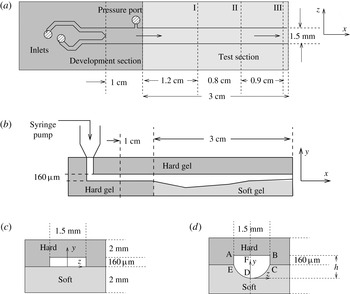
0.55 MPa. The stamp pattern consists of two identical inlets, which converge into one channel of dimensions shown in figure 1(a). Inlet holes are punched into the PDMS stamp, and these are connected to syringe pumps using pipette tips. The fourth wall is prepared as a film of thickness 2 mm of much softer gel with a catalyst concentration 1.75 %, and a shear modulus of
 ${\sim}$
18 kPa. The resulting cross-sectional configuration is shown in figure 1(c). The microchannel is designed so that there is a developing section of
 ${\sim}$
1 cm, where all four walls are made of hard gel, upstream of the test section of length
 ${\sim}$
3 cm where one of the walls is made of soft gel, so that the flow is fully developed before it enters the test section. A side port is also fabricated in the stamp just upstream of the test section, so that the difference in pressure between the entrance of the test section and the outlet (which is open to the atmosphere) can be measured.
The schematic of the top view (a) of the PDMS stamp bonded onto the bottom polymer film, the side view (b) of the deformed channel when there is an applied pressure difference, the channel cross-section in the absence of deformation (c) and when there is deformation due to applied pressure gradient (d). The maximum height
 $h$
is a function of the downstream position, as shown in (b). The locations I, II and III, where the particle image velocimetry measurements are carried out, are shown in (a).

When a pressure gradient is applied, there is a deformation of the bottom soft wall of the microchannel, as shown in figure 1(d). There is very little deformation of the three hard walls made of PDMS with elasticity modulus
 ${\sim}$
0.55 MPa, but there is significant deformation of the bottom soft wall made of PDMS with elasticity modulus 18 kPa.
2.2 Experimental configuration
The microchannel is mounted on an optical table with the flow (
 $x$
) and spanwise (
 $z$
) directions horizontal, and the cross-stream (
 $y$
) direction (with the smallest height of
 ${\sim}$
160
 $\unicode[STIX]{x03BC}\text{m}$
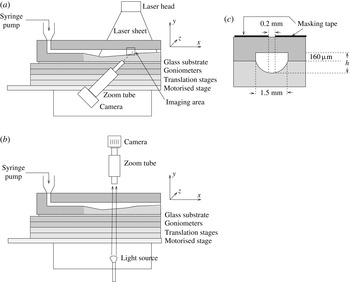
) vertical, as shown in figure 2. Two different configurations are used for imaging in the experiments. The configuration shown in figure 2(a), where the
 $x$
–
 $y$
plane is imaged from the side, is used for measuring the wall deformation discussed in § 2.3, and for the particle image velocimetry (PIV) measurements described in § 2.5. The configuration shown in figure 2(b), where the
 $x$
–
 $z$
plane is imaged from above, is used for the dye-stream experiments, where clear water is pumped though one inlet and water coloured with a dye is pumped through the other inlet, and the mixing of the two streams is observed in the microchannel. The configuration in figure 2(b) is also used for measuring the motion in the bottom wall, by marking the wall with a dye spot and observing the motion of the spot.
The configuration used (a) for the PIV measurements and for determining the channel deformation, and (b) for the dye-stream imaging and the wall oscillations; (c) shows the cross-sectional view of the masking tape used for confining the laser sheet in the PIV measurements.

2.3 Wall deformation
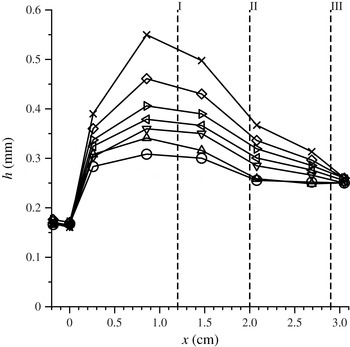
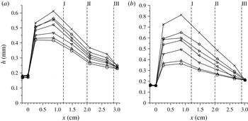
When a pressure difference is applied between the inlet and outlet, there is a deformation of the soft wall of the channel, as shown in figure 1(d). There is very little deformation in the development section, because all four walls are made of hard gel, but there is significant deformation in the test section. The deformation of the wall is measured as a function of the downstream distance using images taken from the side in the configuration shown in figure 2(a), using a Photron FastCam SA-Z camera with an attached Navitar 48X Zoom Tube for magnification. The outline of the channel in the images provides the maximum height along the central plane of the channel shown by the dashed line in figure 1(d). The shape of the bottom wall is then reconstructed using a cubic spline fit at each downstream location. In appendix B, the results for the change in height of the channel due to the applied pressure gradient are presented.
The deformed shape of the channel is reconstructed, and ANSYS FLUENT simulations in the deformed channel are used to determine the velocity profile for the laminar flow of a Newtonian fluid with the same viscosity as the polymer solution. These are then compared with the experimental velocity profiles, to examine whether the flow is laminar. The procedure is as follows.
-
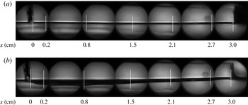
(i) Multiple images of the side of the channel are captured at predefined locations using a zoom tube, and these are combined as shown in figure 3. From this side view, the maximum height of the channel along the central plane in the spanwise direction, the vertical line DF in figure 1(d), is measured. The maximum height is shown as a function of downstream distance in appendix B in figures 23 and 24.
-
(ii) The shape of the deformed bottom surface in figure 1(d) is reconstructed using a cubic spline procedure, from the maximum height DF along the central plane, the undeformed heights AE and BC along the side walls, and the condition that the variation of the height in the
 $z$
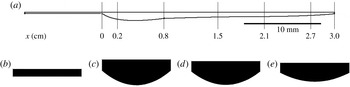
direction is zero by symmetry at the point D. An example of the side view and the cross-section of the reconstructed channel is shown in figure 4.
-
(iii) The deformed cross-section of the channel at each downstream location is then used to reconstruct the three-dimensional channel shape using Autodesk Inventor. The mesh generation in the channel was carried out using Gambit 2.4.6; the smallest spatial dimension in the cross-stream direction was
${\sim}$
20
$\unicode[STIX]{x03BC}\text{m}$
; this level of discretisation required
${\sim}10^{6}$
grid points. The procedure and validation has been discussed earlier in § 3.1 of (Verma & Kumaran Reference Verma and Kumaran2013). -
(iv) The flow simulations were carried out using ANSYS FLUENT 14.0 computational fluid dynamics software, using the laminar flow model for a Newtonian fluid, and the pressure velocity formulation for solving the Navier–Stokes equations. The boundary conditions at all the bounding surfaces were the zero-velocity boundary conditions. The velocity profile was specified to be a plug flow at the inlet to the development section, zero pressure at the outlet and zero velocity as the initial condition. The validation for this procedure is provided in § 3.5 of Srinivas & Kumaran (Reference Srinivas and Kumaran2015), and further details are provided in § 2.2 of Srinivas & Kumaran (Reference Srinivas and Kumaran2015). When compared with a parabolic velocity profile for a laminar flow, the difference between the simulation and analytical results was reported to be
${\sim}$
2 % in Srinivas & Kumaran (Reference Srinivas and Kumaran2015).


The side view, imaged using the configuration in figure 2(a), of the undeformed microchannel (a) and the deformed microchannel for the flow of polyacrylamide solution with molecular weight
 $5\times 10^{6}$
, mass fraction 50 ppm and Reynolds number 406 (b). The streamwise locations where the height was measured are shown by the vertical lines, and
 $x=0$
corresponds to the entrance of the test (soft) section.

Side view (a) and cross-sectional views at different downstream locations in the test section (b) and at locations I (c), II (d) and III (e) (in figure 1 a) of the channel reconstructed from the images in figure 3(b). In (b–e), the width of the channel, which is 1.5 mm, serves as a reference length.

2.4 Dye-stream mixing
In the dye-stream experiments, clear water/polymer solution is pumped through one of the inlets, while water/polymer solution with black coloured Bril ink is pumped through the other inlet, both at equal flow rates. The mixing of the two fluids is recorded using a Photron FastCam SA-Z camera from above in the configuration shown in figure 2(b). In a laminar flow, the two streams flow parallel to each other and there is no motion of the interface. This is because the diffusion time across a width
 $W$
is much longer than the residence time in the channel. The diffusion time, which scales as
 $W^{2}/D$
, is of the order of 2250 s across a width of 1.5 mm, even if we consider a relatively high diffusion coefficient of
 $D=10^{-9}~\text{m}^{2}~\text{s}^{-1}$
for small molecules in water, while the residence time of the fluids in the microchannel is much less than 1 s. Therefore, there is virtually no mixing between the fluid streams in the microchannel in a laminar flow. Motion of the dye across the channel provides evidence of mixing between the two streams.
The mixing is quantified by the following procedure used in Verma & Kumaran (Reference Verma and Kumaran2013), following similar procedures used earlier in Lee, Choi & Park (Reference Lee, Choi and Park2010). The grey scale images of the channel taken from above are processed to determine the grey scale intensity,
 $G_{ij}(t_{k})$
, at each pixel
 $(i,j)$
at the time instant
 $t_{k}$
within a rectangular region. The average intensity and the variance of the intensity at each time instant are
 $$\begin{eqnarray}\displaystyle & \displaystyle G_{av}=\frac{1}{N}\mathop{\sum }_{i,j}G_{ij}, & \displaystyle\end{eqnarray}$$
 $$\begin{eqnarray}\displaystyle & \displaystyle \langle (\unicode[STIX]{x0394}G)^{2}\rangle =\frac{1}{N}\mathop{\sum }_{i,j}(G_{ij}-G_{av})^{2}, & \displaystyle\end{eqnarray}$$
where
 $N$
is the total number of pixels in each frame. The segregation index is obtained by taking the ratio of the r.m.s. of the grey scale intensity fluctuations and dividing it by the maximum difference in the grey scale intensities in the dye and the clear fluid,
 $$\begin{eqnarray}S_{I}=\frac{\sqrt{\langle (\unicode[STIX]{x0394}G)^{2}\rangle }}{G_{w}-G_{d}},\end{eqnarray}$$
where
 $G_{w}$
and
 $G_{d}$
are the grey scale intensities of clear water stream and the dye stream. The segregation index is close to zero if the two streams are fully mixed, and has a maximum of 0.5 when the two streams are perfectly segregated with no lateral mixing. The segregation index is used to quantify the effect of polymer addition on the cross-stream mixing after transition.
For the dye concentrations we have used here, the grey scale intensity is not a linear function of the concentration. When the dye that was initially restricted to one half of the channel mixes throughout the channel, the dye concentration decreases by a factor of
 $2$
, but there is virtually no change in the colour. Thus, the colour cannot be used as a quantitative measure of the concentration. It can only be used to infer the spatial extent to which the dye has mixed into the clear fluid, and to distinguish the extent of mixing for different polymer concentrations. Quantitative measures of mixing have been analysed in an earlier study of Kumaran & Bandaru (Reference Kumaran and Bandaru2016).
The segregation index is calculated at locations I, II and III in figure 1(a), using images of the type shown in figures 5–7 presented in § 3.2.
2.5 Fluid velocity fields
The fluid velocity fields in the
 $x$
–
 $y$
plane (the central plane of the channel in the spanwise (
 $z$
) direction) are measured using PIV with the configuration in figure 2(a). An IDT PIV system, which consists of a SharpVision
 $^{\text{TM}}$
1500-EX charge-coupled device (CCD) camera with spatial resolution of
 $1360\times 1036$
pixels, Nd:YAG laser (Solo-III, New-Wave Research), laser sheet generating optics and a frame rate of 15 Hz, is used for the PIV measurements. The seed particles used for the PIV measurements were prepared using a customised procedure, dispersion polymerisation of styrene in a solution of ethanol (Srinivas & Kumaran Reference Srinivas and Kumaran2015), adapted from Lenzmann et al. (Reference Lenzmann, Li, Kitai and Stover1994). This procedure produces spherical polymer particles of size
 ${\sim}2.12\pm 0.41~\unicode[STIX]{x03BC}\text{m}$
with circularity between 0.95 and 1.0. (
 $4\unicode[STIX]{x03C0}\times \text{area}/\text{perimeter}^{2}$
of the projection of the shape onto a two-dimensional plane.) The size of the particles was carefully selected to ensure that they follow the fluid streamlines (Srinivas & Kumaran Reference Srinivas and Kumaran2015). For particles with size below
 ${\sim}1~\unicode[STIX]{x03BC}\text{m}$
, the Péclet number is small and Brownian diffusion is important, so the particles cross streamlines due to Brownian diffusion. Particles with size greater than
 ${\sim}10~\unicode[STIX]{x03BC}\text{m}$
have high Stokes number, so they cross streamlines due to inertial effects. For the particle size selected here, both Brownian diffusion and inertial effects are small, and so the particles follow the fluid streamlines and the fluid velocity is accurately captured.
For the PIV measurements, a laser sheet is directed downwards along the central plane of the channel using the configuration as shown in figure 2(a), and images are taken using a camera from the side. The laser sheet is confined to a width of
 ${\sim}$
200
 $\unicode[STIX]{x03BC}\text{m}$
along the central plane of the channel in the
 $z$
direction using two masking tapes placed on the channel, as shown in figure 2(c), in order to avoid averaging of the velocity field in the spanwise direction.
The images are captured with a frame rate of 15 image pairs per second. The pulsed laser illumination for each pair of images is separated by a time interval of 10–100 ns depending on the flow speed. The images obtained in the
 $x{-}y$
plane are divided into 60 equal intervals in the cross-stream (
 $y$
) direction. The fluid velocities, calculated from the peak of the autocorrelation function between successive images in each image pair, are assigned to the midpoint of each interval. The mean and r.m.s. velocities are then calculated by averaging over multiple frames. For each set of parameter values, 4000 pairs of images are captured in two sequences of 2000 pairs each. The mean velocity is the average over all 4000 image pairs. In order to assess the variability in the data, the 4000 image pairs are divided into eight subsequences of 500 image pairs each, and the average over each of these subsequences is calculated. The standard deviation is determined from the average of these eight subsequences, and the error bars in the figures show one standard deviation above and below the mean value. The validation of the PIV measurements with the ANSYS FLUENT simulations for the flow of pure water in a deformed channel are shown in figure 7 of Srinivas & Kumaran (Reference Srinivas and Kumaran2015). The validation of the turbulence measurements is shown in the appendix of Srinivas & Kumaran (Reference Srinivas and Kumaran2015) at a Reynolds number of 3500 for the same channel configuration.
2.6 Wall motion
The configuration in figure 2(b) has been used to monitor wall motion. The bottom soft wall of the channel is marked with a dye spot at three different downstream locations along the centreline of the channel in the spanwise direction. The dye spot is irregular and has a linear dimension of between 0.025 and 0.05 mm. The images of the dye spot are captured from above using the Photron FastCam SA-Z camera with a frame rate of 1000
 $\text{frame}~\text{s}^{-1}$
, and the displacement of the centroid of the dye spot in the streamwise (
 $x$
) and spanwise (
 $z$
) directions between successive frames is determined. One pixel in the image corresponds to a linear displacement of
 $0.35~\unicode[STIX]{x03BC}\text{m}$
, and the resolution in the displacement measurements is
 ${\sim}0.5~\unicode[STIX]{x03BC}\text{m}$
.
When there is fluid flow in the channel, there is a mean wall displacement in the spanwise direction,
 $\bar{u}_{x}$
, due to the shear stress exerted by the fluid on the wall. This is measured from the displacement of the dye spot in the streamwise direction observed using a camera above the channel as shown in figure 2(b). There are also displacement fluctuations in the streamwise and spanwise directions due to the fluid turbulence, and the r.m.s. values of these fluctuations are designated
 $u_{x}^{\prime }$
and
 $u_{z}^{\prime }$
, respectively. The variation of the displacement with time is captured, and the Fourier transform of this time series is used to determine the spectra of the displacement fields,
 $\tilde{u} _{x}(\unicode[STIX]{x1D714})$
and
 $\tilde{u} _{z}(\unicode[STIX]{x1D714})$
,
 $$\begin{eqnarray}\tilde{u} _{x}(\unicode[STIX]{x1D714})=\frac{1}{T}\int _{0}^{T}\text{d}t\exp (\text{i}\unicode[STIX]{x1D714}t)u_{x}(t).\end{eqnarray}$$
Since the maximum frame rate is 1000
 $\text{frame}~\text{s}^{-1}$
, the Nyquist frequency is 500
 $\text{frame}~\text{s}^{-1}$
or
 ${\sim}$
3000
 $\text{rad}~\text{s}^{-1}$
. The time period
 $T$
in (2.4) was set equal to 1 s in most experiments, but longer runs up to 30 s have also been used to ensure that there are no systematic low-frequency oscillations.
2.7 Polymer solutions
Solutions of polyacrylamide, with molecular weights
 $4\times 10^{4}$
and
 $5\times 10^{6}$
, procured from Sigma-Aldrich, are used for the experiments. Since the monomer molecular weight is
 ${\sim}$
71, each polymer molecule comprises
 ${\sim}$
560 repeat units for the polymer with molecular weight
 $4\times 10^{4}$
, and
 ${\sim}$
70 500 repeat units for the polymer with molecular weight
 $5\times 10^{6}$
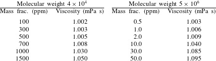
. The solutions are always freshly prepared by dissolving polyacrylamide powder in de-ionised water, since it is known that the rheological properties of polyacrylamide solution could change if it is stored for hours or days (Kulicke, Kniewske & Klein Reference Kulicke, Kniewske and Klein1982). The mass fractions and viscosities of the polymer solutions are provided in table 1.
The mass fractions and the viscosities of the polymer solutions used in the experiments. Addition of polymer causes only small changes in the solution viscosity, but it has a large effect on transition and turbulence, as shown in § 3.

The viscosity measurement was carried out in a Brookfield capillary viscometer, since it is too small to examine in a traditional rheometer. The accuracy depends on the sensitivity of the pressure transducer used to calculate the pressure difference. Even here, the pressure difference is calibrated to that of pure water, and then the change in the pressure difference due to the added polymer is determined. With this, we were able to calculate to within
 $\pm 0.002$
of the viscosity of water. It should be noted that the capillary viscometer is also not ideal for measuring the viscosity of polymers, since there is likely to be polymer extension and contraction at the inlet and outlet. For added verification, we have compared with the viscosity obtained from the specific viscosity reported by Kulicke et al. (Reference Kulicke, Kniewske and Klein1982), which results in a solution viscosity of
 ${\sim}$
1.075 mPa s for the polymer with molecular weight
 $5\times 10^{6}$
at the highest concentration of 50 ppm. Also, Samanta et al. (Reference Samanta, Dubief, Holzner, Schfer, Morozov, Wagner and Hof2013) report a zero-shear viscosity of 1.1 mPa s for a concentration of 50 ppm for the same molecular weight. Therefore, our viscosity of 1.095 mPa s from the Brookfield viscometer is consistent with these.
The relaxation time of the polymers in solution could not be measured directly, since there is very little modification of the water viscosity. The relaxation time has been estimated by different methods, and the values differ significantly depending on the method. In shear-thinning fluids, the Carreau–Yasuda fit for the viscosity versus strain rate is used to estimate the relaxation time. Small-amplitude oscillatory shear measurements can be fitted to a Maxwell model, in order to obtain the longest relaxation time. It is also possible to use the first normal stress difference to estimate the relaxation time (Pan et al. Reference Pan, Morozov, Wagner and Arratia2013) or to use the capillary bridge extensional rheometer, as was done by Samanta et al. (Reference Samanta, Dubief, Holzner, Schfer, Morozov, Wagner and Hof2013).
For polyacrylamide with molecular weight
 $5\times 10^{6}$
, Samanta et al. (Reference Samanta, Dubief, Holzner, Schfer, Morozov, Wagner and Hof2013) report the relaxation time in the range of 1–10 ms by the CaBER method. For the multi-mode Maxwell model, Neelamegam et al. (Reference Neelamegam, Shankar and Das2013) report relaxation times of 2–10 s, while Poole et al. (Reference Poole, Escudier, Afonso and Pinho2007) report relaxation times up to 20 s, so there is a range of
 ${\sim}10^{5}$
in the relaxation times reported by different authors. Zell et al. (Reference Zell, Gier, Rafai and Wagner2010) have analysed the relaxation times calculated by different methods for, among other polymers, polyacrylamide with molecular weight
 ${\sim}5\times 10^{6}$
. They have found that the relaxation time from the Maxwell model is actually the smallest, in the range 1–10 ms. The relaxation time from the viscosity measurements is the largest, in the range 1–100 s, while that from the normal stress differences and capillary extension is in between, in the range 0.1–1 s.
In order to avoid ambiguity, we have defined the relaxation time based on the Zimm model for a polymer in a good solvent (Doi & Edwards Reference Doi and Edwards1988),
 $$\begin{eqnarray}\unicode[STIX]{x1D706}=\frac{\unicode[STIX]{x1D702}_{s}R_{g}^{3}}{k_{B}T},\end{eqnarray}$$
where
 $\unicode[STIX]{x1D702}_{s}$
is the solvent viscosity,
 $R_{g}$
is the radius of gyration and
 $k_{B}T$
is the thermal energy. Defined this way, there is no uncertainty in the definition of the relaxation time, especially since we are in the dilute single-chain limit. Kulicke et al. (Reference Kulicke, Kniewske and Klein1982) report that the end-to-end distance of polyacrylamide molecules of molecular weight
 $5\times 10^{6}$
is
 ${\sim}$
0.5
 $\unicode[STIX]{x03BC}\text{m}$
. This can also be calculated if we consider the Flory characteristic ratio
 $(b/a)^{2}$
of
 ${\sim}$
8.5 (Bohdanecky, Petrus & Sedldtek Reference Bohdanecky, Petrus and Sedldtek1983), where
 $a$
is the monomer size and
 $b$
is the Kuhn segment length. This implies that there are approximately three monomers in each Kuhn segment, and that each Kuhn segment is
 ${\sim}$
10 Å. The relaxation time from (2.5) is then
 ${\sim}$
0.03 s for the polymer with molecular weight
 $5\times 10^{6}$
. For the smaller molecular weight polymer, the ratio of relaxation times scales as
 $M^{1.8}$
, if we consider the radius of gyration to scale as
 $M^{0.6}$
. Based on this, the relaxation time is
 $5\times 10^{-6}$
s for polyacrylamide with molecular weight
 $4\times 10^{4}$
.
2.8 Dimensionless numbers
-
(1) The Reynolds number is defined as
(2.6)where
$$\begin{eqnarray}Re=\frac{\unicode[STIX]{x1D70C}Q}{\unicode[STIX]{x1D702}W},\end{eqnarray}$$
$Q$
is the flow rate,
$W$
is the channel width, and
$\unicode[STIX]{x1D70C}$
and
$\unicode[STIX]{x1D702}$
are the fluid density and viscosity. For a rectangular microchannel, this definition reduces to
$\unicode[STIX]{x1D70C}\bar{v}h/\unicode[STIX]{x1D702}$
, where
$\bar{v}$
is the average velocity (flow rate divided by area of cross-section) and
$h$
is the height. However, the advantage of the definition of
$Re$
in (2.6) is that it is independent of height, and so the Reynolds number does not change when there is channel deformation.
-
(2) The Weissenberg number is defined as
(2.7)where
$$\begin{eqnarray}We=\frac{\unicode[STIX]{x1D706}\bar{v}}{h},\end{eqnarray}$$
$\unicode[STIX]{x1D706}$
is the polymer relaxation time. The ratio of the Weissenberg number and the Reynolds number, denoted as the elasticity number
$El$
, is independent of the flow velocity, (2.8)The relaxation time is
$$\begin{eqnarray}El=\frac{\unicode[STIX]{x1D706}\unicode[STIX]{x1D702}}{\unicode[STIX]{x1D70C}h^{2}}.\end{eqnarray}$$
${\sim}$
0.03 s for polyacrylamide with molecular weight
$5\times 10^{6}$
, and approximately
$5\times 10^{-6}$
s for polyacrylamide with molecular weight
$4\times 10^{4}$
. The channel height varies approximately between
$160~\unicode[STIX]{x03BC}\text{m}$
when there is no flow, to a maximum of
${\sim}500~\unicode[STIX]{x03BC}\text{m}$
at the largest flow rate used here. Based on this, for channels of height
$160{-}500~\unicode[STIX]{x03BC}\text{m}$
, the elasticity number varies between
$1.2$
and
$0.12$
for the polyacrylamide with molecular weight
$5\times 10^{6}$
, and between
$2\times 10^{-5}$
and
$2\times 10^{-4}$
for the polyacrylamide with molecular weight
$4\times 10^{4}$
. However, it should be cautioned that the elasticity number could change by a factor of 10–100 if other measures of the relaxation time based on the rheology are used.
There is deformation of the soft wall in the experiments, and the Weissenberg and elasticity numbers vary with channel height. Therefore, the results are parametrised by the polyacrylamide molecular weight and mass fraction instead of the Weissenberg and elasticity numbers.
-
(3) The fluid–wall interaction is characterised by the dimensionless parameter
$\unicode[STIX]{x1D6F4}=\unicode[STIX]{x1D70C}Gh^{2}/\unicode[STIX]{x1D702}^{2}$
, where
$G$
is the shear modulus of the wall material. The soft wall has a shear modulus of
${\sim}$
18 kPa for all the experiments, and so the parameter
$\unicode[STIX]{x1D6F4}$
is
$4.6\times 10^{5}$
to
$4.6\times 10^{6}$
for water and for
$h$
in the range
$160{-}500~\unicode[STIX]{x03BC}\text{m}$
. The value of
$\unicode[STIX]{x1D6F4}$
decreases by
${\sim}$
20 % for the most viscous polymer solution used here, because the viscosity increases by
${\sim}$
10 %.


3 Results
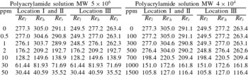
To place the results in context, the transition Reynolds numbers for polymer solutions with different mass fractions at the three locations I, II and III (figure 1 a), are first provided in table 2. After this, the different indicators of transition, such as dye-stream mixing, wall motion and fluid fluctuating velocities, are discussed in detail.
3.1 Transition Reynolds number
Table 2 shows the highest Reynolds number at which the flow is observed to be laminar,
 $Re_{l}$
, the lowest Reynolds number at which the laminar flow is observed to be disrupted,
 $Re_{h}$
, and the average of the two Reynolds numbers,
 $Re_{t}$
, which is designated the transition Reynolds number for the present purposes. At polymer mass fractions below a threshold
 $w_{t}$
, which is 500 ppm and 1 ppm for the solutions of polyacrylamide with molecular weight
 $4\times 10^{4}$
and
 $5\times 10^{6}$
, respectively, the transition Reynolds number is almost the same as that of pure water. The small variation in the transition Reynolds number is due to the slight increase in the viscosity due to polymer addition, as shown in table 1. Above the threshold mass fraction, there is a sharp decrease in the transition Reynolds number, and the transition is observed at a Reynolds number as low as 116 for the solution of polyacrylamide with molecular weight
 $4\times 10^{4}$
and mass fraction 1500 ppm, and as low as
 ${\sim}$
35 for the solution of polyacrylamide with molecular weight
 $5\times 10^{6}$
and mass fraction 50 ppm.
The highest Reynolds number at which the flow is laminar,
 $Re_{l}$
, the lowest Reynolds number at which there is flow disruption,
 $Re_{h}$
, and the arithmetic average of these two, which is considered the transition Reynolds number,
 $Re_{t}$
, as a function of the polymer mass fraction.
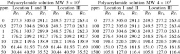
For pure water, transition is observed when the Reynolds number is increased from 277 to 305 at the downstream locations I and II, and from 250 to 277 at the downstream location III. This slight variation is consistent with the earlier experimental results of Verma & Kumaran (Reference Verma and Kumaran2013) and Srinivas & Kumaran (Reference Srinivas and Kumaran2015) for the flow of water in a microchannel, where it was observed that the disruption of the laminar flow first takes place at the downstream locations when the Reynolds number is increased, and then progresses upstream.
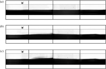
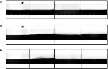
Images of, left to right, the entrance to the test section, location I, location II and location III, in figure 1(a), for the flow of water at Reynolds numbers 250 (a), 305 (b) and 444 (c). The water pumped into the bottom inlet is mixed with black ink for visualisation. The development section is to the left of the arrow, and the test section to the right of the arrow.

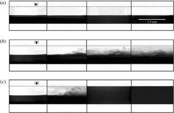
Images of, left to right, the entrance to the test section, location I, location II and location III in figure 1(a), for the flow of a solution of polyacrylamide of molecular weight
 $5\times 10^{6}$
and mass fraction 2 ppm at Reynolds numbers 193 (a), 231 (b) and 441 (c). The solution pumped into the bottom inlet is mixed with black ink for visualisation. The development section is to the left of the arrow, and the test section to the right of the arrow.

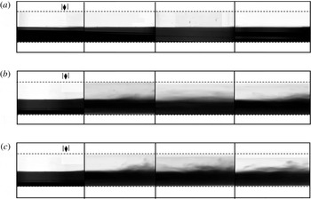
Images of, left to right, the entrance to the test section, location I, location II and location III in figure 1(a), for the flow of a solution of polyacrylamide of molecular weight
 $5\times 10^{6}$
and mass fraction 50 ppm at Reynolds numbers 20 (a), 41 (b) and 101 (c). The solution pumped into the bottom inlet is mixed with black ink for visualisation. The development section is to the left of the arrow, and the test section to the right of the arrow.

It is important to note that there is a significant increase in the height of the microchannel due to the applied pressure gradient. As shown in figure 1(d), there is no discernible deformation of the three hard walls of the microchannel, but there is a significant compression of the soft wall. The height of the microchannel first increases downstream from the start of the developing section (joint between the hard and soft sections in figure 1 b), and then decreases further downstream as the pressure decreases. The deformation is discussed in detail in appendix B.
3.2 Dye-stream mixing
In order to assess the cross-stream mixing, one of the inlet streams (figure 1
a) is mixed with a small amount of black ink, while the other is transparent. The resulting images are shown in figures 5–7 for pure water, for polymer solution of molecular weight
 $5\times 10^{6}$
with mass fraction 2 ppm (just above
 $w_{t}$
) and for the maximum mass fraction 50 ppm. In all cases, images are shown, from left to right, at the entrance to the test section (to verify that there is no disturbance at the inlet) and the three locations I, II and III in figure 1(a). The panels from top to bottom show the images at a Reynolds number below transition, one above transition and a Reynolds number significantly exceeding the transition Reynolds number.
The images in figure 5 show the results for the flow of pure water. No cross-stream mixing is observed below transition. There is intense cross-stream mixing at the downstream locations I, II and III at a Reynolds number of 305, which is higher than the transition Reynolds number, and the extent of mixing increases with downstream distance. The images for polymer solutions with mass fraction just above
 $w_{t}$
are shown in figure 6. In this case, there is no mixing below the transition Reynolds number, but cross-stream mixing is observed when the transition Reynolds number is exceeded. However, the mixing is clearly imperfect, and the mixing intensities are significantly lower than those for pure water. Complete cross-stream mixing is not observed even at the highest experimental Reynolds numbers of
 ${\sim}$
400. In figure 7, the polymer mass fraction is increased to 50 ppm for the polyacrylamide with molecular weight
 $5\times 10^{6}$
. In this case, there is very little cross-stream mixing. However, fluctuations at the interface are clearly observed when the transition Reynolds number is exceeded, and in video recordings, motion of the interface between the transparent and coloured fluid is clearly visible, indicating that there is an instability of the laminar flow.
The segregation index
 $S_{I}$
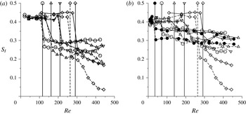
, defined in (2.3), is shown as a function of Reynolds number in figure 8 at two locations, I and III. For pure water, the segregation index is close to 0.5 when the Reynolds number is below
 $Re_{t}$
, and it decreases steeply when the Reynolds number crosses
 $Re_{t}$
. The segregation index is lower at the downstream location III in comparison to the upstream location I, indicating greater mixing at the downstream location, as observed in figure 5. The results for mass fractions below
 $w_{t}$
are qualitatively similar to that for water; these are not shown in figure 8 in order to enhance clarity. When the mass fraction increases beyond
 $w_{t}$
, two effects are clearly visible. Firstly, there is a decrease in the transition Reynolds number at which
 $S_{I}$
decreases sharply. Secondly, the segregation index is higher than that for pure water, and it increases with polymer mass fraction. At the highest mass fraction of 50 ppm for the polyacrylamide with molecular weight
 $5\times 10^{6}$
, the segregation index decreases to
 ${\sim}$
0.35 at location I and 0.3 at location III, indicating that the mixing is very imperfect; this is evident in the images in figure 7, where there is poor mixing even at the downstream location III. There is better mixing for the polyacrylamide with molecular weight
 $4\times 10^{4}$
at the highest mass fraction of 1500 ppm, but, even here, the segregation index decreases to
 ${\sim}$
0.25 at location I and 0.2 at location III. This is much higher than the minimum value of
 ${\sim}$
0.05 at the location III for pure water.
The segregation index
 $S_{I}$
(2.3) as a function of the Reynolds number
 $Re$
at locations I (solid line) and III (dashed line) for (a) a solution of polyacrylamide with molecular weight
 $4\times 10^{4}$
and mass fraction 1500 ppm (○), 1000 ppm (▵) and 700 ppm (▿), and (b) a solution of polyacrylamide with molecular weight
 $5\times 10^{6}$
and mass fraction 50 ppm (●), 30 ppm (○), 10 ppm (▵) and 2 ppm (▿). The results for pure water are shown by the ♢ symbols in both panels. The vertical solid and dashed lines show the transition Reynolds numbers at location I and III, respectively, for different polymer concentrations.

3.3 Flow dynamics
The results for the mean and fluctuating velocities are shown in figures 9–12. Results are shown for four Reynolds numbers, two below transition, the third just above the transition Reynolds number and the fourth much higher than the transition Reynolds number. Only the results at location II are shown in all the figures; the results at other locations are qualitatively similar. In all these figures, the bottom wall is located at
 $y=0$
, while the location of the top wall is indicated by the vertical dashed lines. The change in position of the top wall is due to the increase in height as the Reynolds number increases. It is important to reiterate that we have not been able to make velocity measurements within a distance of
 ${\sim}15~\unicode[STIX]{x03BC}\text{m}$
from the bottom wall, due to reflection of the PIV laser from the bottom wall, and so we do not have a direct measurement of the velocities at the bottom wall. Therefore, results for the fluctuating velocity within a distance of
 ${\sim}$
15
 $\unicode[STIX]{x03BC}\text{m}$
from the wall are not shown, and the results for the mean velocity at the wall are extrapolated to zero velocity. In the figures 9–12, the absolute mean and fluctuating velocities before and after transition are discussed; this is not a measure of the relative magnitudes of the fluctuations to the mean velocity. In the following figures 14 and 15, the dimensionless measures of the mean and fluctuating velocities are shown and discussed.
The mean velocity
 $\bar{v}_{x}$
as a function of the cross-stream distance
 $y$
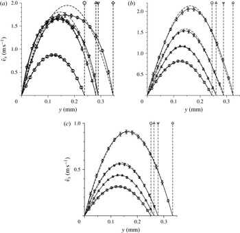
for pure water (a), and for a solution of polyacrylamide with molecular weight
 $5\times 10^{6}$
and mass fraction 2 ppm (b) and 50 ppm (c) at location II (in figure 1
a). In (a), the Reynolds numbers are
 $Re=133$
(○),
 $277$
(▵),
 $305$
(▿) and
 $388$
(♢). In (b),
 $Re=133$
(○),
 $178$
(▵),
 $211$
(▿) and
 $333$
(♢). In (c),
 $Re=20.29$
(○),
 $30.44$
(▵),
 $40.59$
(▿) and
 $121.8$
(♢). The symbols and solid lines are the experimental profiles and the dashed lines are the results of ANSYS FLUENT simulations for the laminar flow of a Newtonian fluid in a channel of the same shape at the same flow rate. The bottom wall is at
 $y=0$
, and the dashed lines on the right show the location of the top wall at different Reynolds numbers.

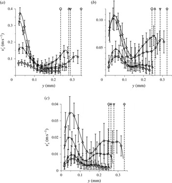
The r.m.s. of the fluctuating velocity
 $v_{x}^{\prime }$
as a function of the cross-stream distance
 $y$
for pure water (a), and for a solution of polyacrylamide with molecular weight
 $5\times 10^{6}$
and mass fraction 2 ppm (b) and 50 ppm (c) at location II (in figure 1
a). In (a), the Reynolds numbers are
 $Re=133$
(○),
 $277$
(▵),
 $305$
(▿) and
 $388$
(♢). In (b),
 $Re=133$
(○),
 $178$
(▵),
 $211$
(▿) and
 $333$
(♢). In (c),
 $Re=20.29$
(○),
 $30.44$
(▵),
 $40.59$
(▿) and
 $121.8$
(♢). The bottom wall is at
 $y=0$
, and the dashed lines on the right show the location of the top wall at different Reynolds numbers.

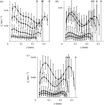
The r.m.s. of the fluctuating velocity
 $v_{y}^{\prime }$
as a function of the cross-stream distance
 $y$
for pure water (a), and for a solution of polyacrylamide with molecular weight
 $5\times 10^{6}$
and mass fraction 2 ppm (b) and 50 ppm (c) at location II (in figure 1
a). In (a), the Reynolds numbers are
 $Re=133$
(○),
 $277$
(▵),
 $305$
(▿) and
 $388$
(♢). In (b),
 $Re=133$
(○),
 $178$
(▵),
 $211$
(▿) and
 $333$
(♢). In (c),
 $Re=20.29$
(○),
 $30.44$
(▵),
 $40.59$
(▿) and
 $121.8$
(♢). The bottom wall is at
 $y=0$
, and the dashed lines on the right show the location of the top wall at different Reynolds numbers.

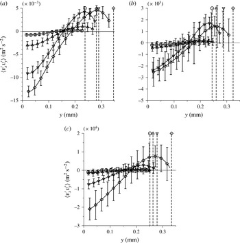
The correlation
 $\langle v_{x}^{\prime }v_{y}^{\prime }\rangle$
as a function of the cross-stream distance
 $y$
for pure water (a), and for a solution of polyacrylamide with molecular weight
 $5\times 10^{6}$
and mass fraction 2 ppm (b) and 50 ppm (c) at location II (in figure 1
a). In (a), the Reynolds numbers are
 $Re=133$
(○),
 $277$
(▵),
 $305$
(▿) and
 $388$
(♢). In (b),
 $Re=133$
(○),
 $178$
(▵),
 $211$
(▿) and
 $333$
(♢). In (c),
 $Re=20.29$
(○),
 $30.44$
(▵),
 $40.59$
(▿) and
 $121.8$
(♢). The bottom wall is at
 $y=0$
, and the dashed lines on the right show the location of the top wall at different Reynolds numbers.

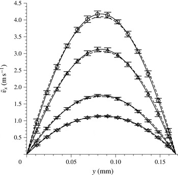
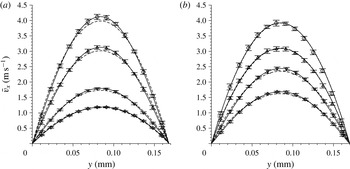
The mean velocity profiles at different Reynolds numbers are compared in figure 9 for the flow of pure water, and polymer solutions of molecular weight
 $5\times 10^{6}$
with mass fraction 2 ppm just above
 $w_{t}$
and the maximum mass fraction of 50 ppm. In this figure, the velocity profiles for a laminar flow obtained using the ANSYS FLUENT computational fluid dynamics software for the same channel shape and flow velocity are shown by the dashed lines. The velocity profiles are in close agreement with the computed velocity profiles for a laminar flow below the transition Reynolds number in table 2, but there is a clear difference between the experimental velocity profile and the laminar profile when the transition Reynolds number is exceeded. For flow of pure water in figure 9(a), it is observed that the experimental velocity profile is in quantitative agreement with that from the ANSYS FLUENT simulations for a laminar flow up to a Reynolds number of 277. When the Reynolds number is increased to 305, the velocity profile is distinctly different from the laminar profiles obtained in the simulations, with a smaller curvature at the centre and sharper gradients at the walls. It is shown a little later that the quantitative measure of the departure from a laminar profile,
 $\bar{v}_{diff}$
, defined in (3.1), exhibits a discontinuous increase at this transition point. For the flow of a solution of polyacrylamide of molecular weight
 $5\times 10^{6}$
and mass fraction 2 ppm, figure 9(b) shows that the velocity profile is in close agreement with the laminar profile for a Newtonian fluid for Reynolds number up to 178, but there is a distinct departure from the laminar profile at a Reynolds number of 211 and higher. It is also evident from figure 9(b) that the extent of departure from the laminar profile is lower for the polymer solution than for pure water in figure 9(a). When the polymer concentration is further increased to 50 ppm, the velocity profiles appear to be close to the laminar profiles at all Reynolds numbers. However, a closer examination of figure 9(c) suggests that there is a small but discernible departure of the profile from the laminar profile when the Reynolds number is increased from
 ${\sim}$
30 to
 ${\sim}$
40. This distinction will also be evident in the discussion of the measure
 $\bar{v}_{diff}$
in figures 14 and 15. Based on figure 9, it can be concluded that there is a significant decrease in the Reynolds number for transition when the polymer mass fraction is 2 ppm or higher, and there is also a significant decrease in the departure of the velocity profile from the laminar profile.
The profiles of the r.m.s. of the velocity fluctuations,
 $v_{x}^{\prime }$
and
 $v_{y}^{\prime }$
, are shown in figures 10 and 11. It is important to reiterate that, in the experiments, there is a non-zero level of fluctuations even in the laminar flow, and this level of fluctuations also decreases significantly as the polymer mass fraction is increased. For pure water, the streamwise r.m.s. velocity
 $v_{x}^{\prime }$
is
 ${\sim}$
15 % of the average velocity, but this decreases to
 ${\sim}$
5 % of the average velocity for the highest polymer mass fractions used here. Similarly, the r.m.s. velocity in the cross-stream direction
 $v_{y}^{\prime }$
is
 ${\sim}$
3 % of the average velocity for pure water, but it decreases to
 ${\sim}$
1 % of the average velocity for the highest polymer mass fractions used here. Thus, the addition of polymer appears to have a significant damping effect on the fluctuations in the laminar flow as well.
Corresponding to the departure of the mean velocity profile from the laminar profile in figure 9, there is also a distinct increase in the amplitude of the velocity fluctuations in figures 10 and 11. The profiles are also asymmetric, and the amplitude of the fluctuations near the bottom (soft) wall is higher by a factor of
 $2$
in comparison to that near the top (hard) wall. This indicates that the soft wall has a significant role to play in the generation of turbulent fluctuations. Most importantly, there is a significant increase in the amplitude of
 $v_{x}^{\prime }$
and
 $v_{y}^{\prime }$
, by more than a factor of
 $2$
, when the Reynolds number exceeds the transition Reynolds number shown in table 2 at each polymer mass fraction. This coincides with the Reynolds number at which the velocity profile shows a distinct departure from the laminar profile in figure 9, indicating that the transition is accompanied by a distinct shift in the form of the velocity profile as well as a significant increase in the amplitude of the fluctuations in both the streamwise and the cross-stream directions.
There is a decrease in the amplitude of the fluctuations in both the streamwise and cross-stream directions as the polymer concentration is decreased. The maximum of
 $v_{x}^{\prime }$
decreases by a factor of 3 in
 $v_{x}^{\prime }$
when the polymer concentration is increased from 0 ppm to 2 ppm and another factor of 3 when the polymer concentration is decreased to 50 ppm.
The profiles of the correlation
 $\langle v_{x}^{\prime }v_{y}^{\prime }\rangle$
at different polymer concentrations are shown in figure 12. This correlation is related to the Reynolds stress
 $\unicode[STIX]{x1D70F}_{xy}^{R}$
by the relation
 $\unicode[STIX]{x1D70F}_{xy}^{R}=-\unicode[STIX]{x1D70C}\langle v_{x}^{\prime }v_{y}^{\prime }\rangle$
, where the Reynolds stress is the rate of transport of momentum due to the turbulent velocity fluctuations. For pure water, when the Reynolds number is below 277, there is a background level of Reynolds stress fluctuations even in the laminar flow. However, at the Reynolds number of 305, there is a sharp increase in
 $\langle v_{x}^{\prime }v_{y}^{\prime }\rangle$
by a factor of
 $3$
. When the polymer concentration is increased, there is a significant decrease in
 $\langle v_{x}^{\prime }v_{y}^{\prime }\rangle$
, as shown in figure 12, by a factor of
 ${\sim}5$
when the polymer mass fraction is increased from 0 ppm to 2 ppm, and a factor of 10 when the polymer mass fraction is increased from 2 ppm to 50 ppm. For each polymer concentration, there is a sharp increase in
 $\langle v_{x}^{\prime }v_{y}^{\prime }\rangle$
, by a factor of
 $3$
or more, when the Reynolds number exceeds the transition Reynolds number listed in table 2. Thus, the indicators of a transition are consistently observed in the mean velocity as well as the r.m.s. fluctuating velocity at the same transition Reynolds number where cross-stream mixing is observed in the dye-stream experiments.
The value of
 $\langle v_{x}^{\prime }v_{y}^{\prime }\rangle$
appears to extrapolate to zero at the top (hard) wall, as required by the condition that the velocity fluctuations should decrease to zero at the wall. However, at the bottom wall, it is difficult to extrapolate these to zero, indicating that the fluctuations at the soft surface may be non-zero. A similar feature was observed for pure water in Srinivas & Kumaran (Reference Srinivas and Kumaran2015). As noted in the first paragraph of this section, we do not have direct measurements of the mean and fluctuating velocities within a distance of
 ${\sim}15~\unicode[STIX]{x03BC}\text{m}$
from the walls. The fluctuating velocities
 $v_{x}^{\prime }$
and
 $v_{y}^{\prime }$
in figures 10 and 11 could plausibly be extrapolated to zero at the bottom wall. However, it is very difficult to extrapolate
 $\langle v_{x}^{\prime }v_{y}^{\prime }\rangle$
to zero at the wall. More sophisticated measurements are required to determine the exact nature of the fluctuations at the wall and in the near-wall region.
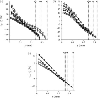
Figure 13 shows the viscous stress (dashed lines) and total stress (solid lines) as a function of the cross-stream distance. For a proper interpretation of this figure, it is important to clearly specify the procedure used for calculating these stresses. The viscous stress is defined as
 $\unicode[STIX]{x1D70F}_{xy}^{v}=\unicode[STIX]{x1D702}(\text{d}\bar{v}_{x}/\text{d}y)$
, where
 $\unicode[STIX]{x1D702}$
is considered a constant equal to the viscosity of the polymer solution. Here, the velocity gradient
 $(\text{d}\bar{v}_{x}/\text{d}y)$
is measured by numerically taking the derivative of the mean velocity profile using a second-order central difference scheme. The total stress is the sum of the viscous and the Reynolds stresses,
 $\unicode[STIX]{x1D70F}_{xy}=\unicode[STIX]{x1D702}(\text{d}\bar{v}_{x}/\text{d}y)-\unicode[STIX]{x1D70C}\langle v_{x}^{\prime }v_{y}^{\prime }\rangle$
. The error bars in the stress calculations are primarily due to the error bars in the correlation
 $\langle v_{x}^{\prime }v_{y}^{\prime }\rangle$
, since the errors in the derivative of the mean velocity are much smaller. For pure water (figure 13
a), there is very little difference between the total and viscous stresses when the Reynolds number is below the transition Reynolds number. However, there is a significant difference above the transition Reynolds number, due to the contribution of the Reynolds stress. This Reynolds stress contribution decreases to zero at the upper hard wall, but is significant at the lower soft wall. The stress is close to a linear function of the cross-stream distance below the transition Reynolds number, as expected for a rigid channel when the pressure gradient is a constant. The stress does depart from a linear function at higher Reynolds numbers due to the channel deformation. However, it should be noted that the viscous stress departs significantly from a linear function of
 $y$
. It is necessary to add the Reynolds stress, which is non-zero at the soft wall, to the viscous stress in order to obtain a total stress profile that is closer to a linear function of cross-stream distance.
The total stress
 $\unicode[STIX]{x1D70F}_{xy}$
(solid lines) and the viscous stress
 $\unicode[STIX]{x1D70F}_{xy}=\unicode[STIX]{x1D702}(\text{d}\bar{v}_{x}/\text{d}y)$
(dashed lines) as a function of the cross-stream distance
 $y$
for pure water (a), and for a solution of polyacrylamide with molecular weight
 $5\times 10^{6}$
and mass fraction 2 ppm (b) and 50 ppm (c) at location II (in figure 1
a). In (a), the Reynolds numbers are
 $Re=133$
(○),
 $277$
(▵),
 $305$
(▿) and
 $388$
(♢). In (b),
 $Re=133$
(○),
 $178$
(▵),
 $211$
(▿) and
 $333$
(♢). In (c),
 $Re=20.29$
(○),
 $30.44$
(▵),
 $40.59$
(▿) and
 $121.8$
(♢). The bottom wall is at
 $y=0$
, and the dashed lines on the right show the location of the top wall at different Reynolds numbers. To enhance clarity, only the error bars for the highest Reynolds number are shown.

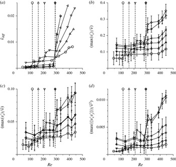
The measure
 $\bar{v}_{diff}$
of the departure of the velocity profile from the laminar profile (a), and the scaled maximum of the velocity fluctuations
 $\max (v_{x}^{\prime })/\bar{v}$
(b),
 $\max (v_{y}^{\prime })/\bar{v}$
(c) and
 $\max (\langle |v_{x}^{\prime }v_{y}^{\prime }|\rangle )/\bar{v}^{2}$
(d), all at location II (in figure 1
a), for a solution of polyacrylamide with molecular weight
 $4\times 10^{4}$
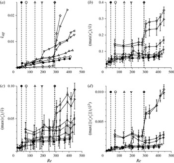
and with mass fraction 1500 ppm (○), 1000 ppm (▵), 700 ppm (▿), 500 ppm (◃), 100 ppm (▹) and pure water (♢). The vertical dashed lines show the transition Reynolds numbers (table 2) at different polymer concentrations.

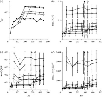
The measure
 $\bar{v}_{diff}$
of the departure of the velocity profile from the laminar profile (a), and the scaled maximum of the velocity fluctuations
 $\max (v_{x}^{\prime })/\bar{v}$
(b),
 $\max (v_{y}^{\prime })/\bar{v}^{2}$
(c) and
 $\max (\langle |v_{x}^{\prime }v_{y}^{\prime }|\rangle )/\bar{v}$
(d), all at location II (in figure 1
a), for a solution of polyacrylamide with molecular weight
 $5\times 10^{6}$
and with mass fraction 50 ppm (●), 30 ppm (○), 10 ppm (▵), 2 ppm (▿), 1 ppm (◃), 0.5 ppm (▹) and pure water (♢). The vertical dashed lines show the transition Reynolds numbers (table 2) at different polymer concentrations.

At the highest polymer mass fraction considered in figure 13(c), the stress profiles are linear functions of cross-stream distance. This is because the transition Reynolds number is low, and the channel deformation is small at the Reynolds numbers under consideration. Moreover, the linear variation of the stress with cross-stream distance indicates that the fluid viscosity can be considered a constant across the channel. At the polymer mass fraction just above
 $w_{t}$
in figure 13(b), the difference between the total stress and viscous stress is comparable to the experimental error bars when the Reynolds number is less than
 $Re_{t}$
, but there is a difference between the total and viscous stresses when the Reynolds number is greater than
 $Re_{t}$
. Thus, there is a discernible contribution to the total stress due to velocity fluctuations.
An important point to note is that the stress profiles are not linear functions of cross-stream distance in figure 13(b). Moreover, the curvature of the stress profiles is the opposite of that expected due to channel deformation, shown in figure 13(a) for pure water. This is possibly related to the non-uniform viscosity of the fluid across the channel, a phenomenon also observed in the flow through a rigid channel considered in appendix A at polymer mass fractions just above
 $w_{t}$
. A close examination of the velocity profiles for the flow through rigid and flexible channels suggests a higher viscosity near the walls and a lower viscosity near the centre. This is the opposite of a shear-thinning effect or shear-induced migration, where the viscosity is expected to be lower at the walls (where the strain rate is higher) and higher at the centre (where the strain rate is zero). One possible explanation is migration of polymers from centre to the walls, resulting in slight variations of the viscosity. The other possibility is shear-thickening due to finite extensibility or due to association between polymers at very high shear rates (Hatzikiriakos & Vlassopoulos Reference Hatzikiriakos and Vlassopoulos1996). This effect, which requires further study possibly by direct measurement of polymer mass fraction, is numerically small but discernible in both hard- and soft-walled channels. Since the computation of the stress assumes a constant viscosity, we find that the stress is no longer linear, but the magnitude of the slope of the
 $\unicode[STIX]{x1D70F}_{xy}$
–
 $y$
curve seems to decrease near the walls. This subtle effect is similar to that of added polymers on the solution viscosity, which is also small but discernible. However, this has a significant effect on the transition, and the flow dynamics in a turbulent flow.
Next, we discuss quantitative measures of the departure from a laminar flow as a function of the Reynolds number. The departure from the mean velocity is characterised by the measure
 $\bar{v}_{diff}$
, defined as
 $$\begin{eqnarray}\bar{v}_{diff}=\sqrt{\frac{1}{v_{x}^{(p)2}h}\int _{0}^{h}\text{d}y\,(\bar{v}_{x}-\bar{v}_{x}^{(l)})^{2}},\end{eqnarray}$$
where
 $\bar{v}_{x}(y)$
is the experimental measurement,
 $\bar{v}_{x}^{(l)}(y)$
is the laminar velocity profile from the ANSYS FLUENT simulations for a channel of the same shape and with the same flow rate as in the experiments, and
 $\bar{v}_{x}^{(p)}$
is the profile-averaged velocity,
 $$\begin{eqnarray}\bar{v}_{x}^{(p)}=\frac{1}{h}\int _{0}^{h}\bar{v}_{x}\,\text{d}y.\end{eqnarray}$$
The fluctuations are characterised by the scaled fluctuation intensities,
 $\text{max}(v_{x}^{\prime })/\bar{v}$
,
 $\text{max}(v_{y}^{\prime })/\bar{v}$
and
 $\text{max}(|\langle v_{x}^{\prime }v_{y}^{\prime }\rangle |)/\bar{v}^{2}$
, where
 $\text{max}(\star )$
is the maximum value of
 $\star$
across the channel, and the mean velocity
 $\bar{v}$
is the ratio of the flow rate and the cross-sectional area.
Figures 14(a) and 15(a) show
 $\bar{v}_{diff}$
as a function of Reynolds number for different polymer mass fractions. This measure
 $\bar{v}_{diff}$
is numerically small when the flow is laminar, but it exhibits a sharp increase by a factor of 1.5–2 at transition, indicating a qualitative change in the form of the velocity profile. The difference between the experimental and laminar profiles decreases systematically with an increase in the polymer mass fraction. However, a sharp change in the value of
 $\bar{v}_{diff}$
is evident at the transition Reynolds number for all values of the polymer mass fraction.
Figures 14(b–d) and 15(b–d) show the maximum values of
 $v_{x}^{\prime }$
,
 $v_{y}^{\prime }$
and
 $|\langle v_{x}^{\prime }v_{y}^{\prime }\rangle |$
across the channel, scaled by suitable powers of
 $\bar{v}$
as a function of the Reynolds number. At transition, there is a discontinuous change in
 $\max (v_{x}^{\prime })/\bar{v}$
,
 $\max (v_{y}^{\prime })/\bar{v}$
and
 $\max (|\langle v_{x}^{\prime }v_{y}^{\prime }\rangle |)/\bar{v}^{2}$
for all values of the polymer mass fraction. For the solution of polyacrylamide with molecular weight
 $4\times 10^{4}$
,
 $\max (v_{x}^{\prime })/\bar{v}$
and
 $\max (v_{y}^{\prime })/\bar{v}$
decrease by
 ${\sim}$
30 % when the polymer mass fraction is increased from 0 ppm to 500 ppm, and the correlation
 $\max (\langle v_{x}^{\prime }v_{y}^{\prime }\rangle )/\bar{v}^{2}$
decreases by more than 50 %. For the solution of polyacrylamide with molecular weight
 $5\times 10^{6}$
, there is a larger decrease of
 ${\sim}$
50 % in
 $\max (v_{x}^{\prime })/\bar{v}$
and
 $\max (v_{y}^{\prime })/\bar{v}$
, and
 ${\sim}$
80 % reduction in
 $\max (\langle v_{x}^{\prime }v_{y}^{\prime }\rangle )/\bar{v}^{2}$
when the polymer mass fraction is increased from 0 ppm to 1 ppm. When the polymer mass fraction exceeds the threshold value, there is a further decrease in the amplitude of the fluctuations, accompanied by a decrease in the transition Reynolds number. At the highest polymer mass fractions, the values of
 $\max (v_{x}^{\prime })/\bar{v}$
and
 $\max (v_{y}^{\prime })/\bar{v}$
are lower by a factor of
 $5$
, and the value of
 $\max (\langle v_{x}^{\prime }v_{y}^{\prime }\rangle )/\bar{v}^{2}$
is lower by a factor of
 $10$
, in comparison to that of pure water. Even at the highest polymer mass fractions studied here, there is a sharp increase by a factor of
 ${\sim}2$
in
 $\max (v_{x}^{\prime })/\bar{v}$
and
 $\max (v_{y}^{\prime })/\bar{v}$
and a factor of
 $4$
in
 $\max (\langle v_{x}^{\prime }v_{y}^{\prime }\rangle )/\bar{v}^{2}$
at transition. This increase is observed at a Reynolds number as low as 139 for the polymer solution with molecular weight
 $4\times 10^{4}$
and mass fraction 1500 ppm, and as low as 35 for the polymer solution with molecular weight
 $5\times 10^{6}$
and mass fraction 50 ppm.
3.4 Wall motion
The displacement of a dye spot marked on the bottom wall at location II in the streamwise direction,
 $\bar{u}_{x}$
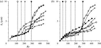
, is shown in figure 16. It should be noted that the mean displacement is proportional to the mean shear stress at the wall, if linear elasticity is used to model the displacement within the wall medium. Figure 16 shows that there is a distinct change in the slope of the graphs of
 $\bar{u}_{x}$
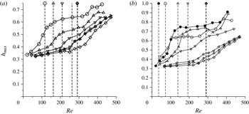
versus Reynolds number at transition for all values of the polymer mass fraction considered here. This is consistent with the slopes of the curves of the maximum height with Reynolds number in figure 25 in appendix B. The mean displacement and the shear stress first decrease as the polymer mass fraction increases, and then increase when the mass fraction increases beyond
 $w_{t}$
. As the polymer mass fraction is increased, the height of the channel first increases, resulting in a lower strain rate for the same flow rate. As the mass fraction is further increased, there is an increase both in the area of cross-section and in the viscosity; the combination of these two effects results in a net increase in the wall shear stress and consequently the wall displacement.
The mean wall displacement as a function of the Reynolds number
 $Re$
for (a) polymer with molecular weight
 $4\times 10^{4}$
and mass fraction 1500 ppm (○), 1000 ppm (▵), 700 ppm (▿), 300 ppm (◃) and 100 ppm (▹), and (b) polymer with molecular weight
 $5\times 10^{6}$
and mass fraction 50 ppm (●), 30 ppm (○), 10 ppm (▵), 2 ppm (▿), 1 ppm (◃) and 0.5 ppm (▹). The results for pure water are shown by the ♢ symbols in both panels. The vertical dashed lines show the transition Reynolds numbers (table 2) at different polymer concentrations as indicated by the symbols.

The r.m.s. of the wall displacement fluctuations in the streamwise direction,
 $u_{x}^{\prime }$
, is shown in figure 17. The r.m.s. of the displacement in the spanwise direction,
 $u_{z}^{\prime }$
, is
 ${\sim}$
25 % smaller than
 $u_{x}^{\prime }$
, but it has the same qualitative characteristics, and so it is not shown separately. For pure water and for low polymer mass fraction below
 $w_{t}$
, the variation of
 $u_{x}^{\prime }$
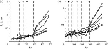
with the Reynolds number is in agreement with the earlier study of Srinivas & Kumaran (Reference Srinivas and Kumaran2015). A baseline fluctuation level is observed even in a laminar flow due to experimental noise, but there is a sharp increase in the level of fluctuations at transition in both the streamwise and spanwise directions, confirming the onset of wall motion along with the fluctuations in the fluid. As the polymer concentration was increased, the magnitude of the fluctuations decreased below the detection limit in our experiments, which is
 ${\sim}0.5~\unicode[STIX]{x03BC}\text{m}$
, and so we were not able to detect a change in the fluctuations.
The r.m.s. of the fluctuations in the wall displacement as a function of the Reynolds number
 $Re$
for (a) polymer with molecular weight
 $4\times 10^{4}$
and mass fraction 1500 ppm (○), 1000 ppm (▵), 700 ppm (▿), 300 ppm (◃) and 100 ppm (▹), and (b) polymer with molecular weight
 $5\times 10^{6}$
and mass fraction 50 ppm (●), 30 ppm (○), 10 ppm (▵), 2 ppm (▿), 1 ppm (◃) and 0.5 ppm (▹). The results for pure water are shown by the ♢ symbols in both panels. The vertical dashed lines show the transition Reynolds numbers (table 2) at different polymer concentrations as indicated by the symbols.

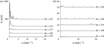
The frequency spectrum of the fluctuations has also been examined in the range of 0–500
 $\text{rad}~\text{s}^{-1}$
at low polymer concentrations. It should be noted that the fluctuations were measured using a high-speed imaging system with a frame rate of 1000
 $\text{frame}~\text{s}^{-1}$
, and so the Nyquist frequency for the measurements is
 ${\sim}$
500
 $\text{frame}~\text{s}^{-1}$
, or
 ${\sim}$
3000
 $\text{rad}~\text{s}^{-1}$
. The measurements have been restricted to
 ${\sim}$
500
 $\text{rad}~\text{s}^{-1}$
in order to provide adequate oversampling. The low-frequency structure in the spectrum is evident in figure 18(a) for the flow of pure water, and is similar to the results reported in Srinivas & Kumaran (Reference Srinivas and Kumaran2015). There is no sharp maximum in the range 0–500
 $\text{rad}~\text{s}^{-1}$
, and there is no clear scaling in with frequency, but the appearance of a broad spectrum at frequencies less then 100
 $\text{rad}~\text{s}^{-1}$
is observed in the experiments. When the polymer concentration is increased just above the threshold concentration, the amplitude of the spectrum decreases significantly, as shown in figure 18(b), and we do not observe any coherent spectrum. This is probably because the amplitude of the velocity fluctuations has decreased below
 ${\sim}$
0.5
 $\unicode[STIX]{x03BC}\text{m}$
, which is the limit of resolution of our optical measurement technique. A similar result is obtained when the polymer concentration is further increased. More advanced techniques for the measurement of displacement fluctuations are required in order to detect the low-amplitude fluctuations for polymer solutions.
The spectra of the streamwise wall displacement,
 $\tilde{u} _{x}$
, at different Reynolds numbers for r.m.s. of the fluctuations in the wall displacement as a function of the Reynolds number for pure water (a) and a solution of polyacrylamide with molecular weight
 $5\times 10^{6}$
and mass fraction 2 ppm (b). Vertical offsets are added to the baselines at different Reynolds numbers to distinguish the different curves.

4 Conclusions
The primary result of the experimental analysis is that polymer addition has two types of effects on transition and turbulence in a soft-walled microchannel.
-
(1) When the polymer mass fraction is below a threshold value
$w_{t}$
, there is a reduction in the turbulence intensities after transition, but there is no change in the transition Reynolds number. The value of
$w_{t}$
is
${\sim}$
1 ppm for the polyacrylamide with molecular weight
$5\times 10^{6}$
, and
${\sim}$
500 ppm for the polymer with molecular weight
$4\times 10^{4}$
. The turbulence reduction is significant. When scaled by suitable powers of the average flow velocity, the dimensionless streamwise and cross-stream r.m.s. velocities decrease by a factor of
$2$
, and the correlation
$\langle v_{x}^{\prime }v_{y}^{\prime }\rangle$
(scaled by the square of the average velocity) decreases by a factor of
$4$
, when the polymer weight fraction increases from 0 to
$w_{t}$
. -
(2) There is a systematic decrease in the transition Reynolds number with increasing mass fraction when the polymer concentration increases beyond
$w_{t}$
. For the highest mass fraction of 1500 ppm for the polymer of molecular weight
$4\times 10^{4}$
, the transition Reynolds number is
${\sim}$
139, and for the highest mass fraction of 50 ppm for the polymer of molecular weight
$5\times 10^{6}$
, the transition Reynolds number is
${\sim}$
35. This is in contrast to the transition Reynolds number of
${\sim}$
291 when the mass fraction is below
$w_{t}$
. The decrease in the transition Reynolds number is accompanied by a significant decrease in the scaled turbulence intensities, by a factor of 5 for the streamwise and cross-stream velocity fluctuations, and by a factor of more than 10 for the correlation
$\langle v_{x}^{\prime }v_{y}^{\prime }\rangle$
, in comparison to pure water. -
(3) The turbulence damping results in very poor cross-stream mixing even at very small polymer concentrations.


There are three other incidental observations which may be of relevance in microfluidics and in the flow of polymer solutions.
-
(i) It is observed that addition of small amounts of polymers causes a significant damping of fluctuations even in the laminar flow. In the flow configurations used here and in many other microfluidic devices, the inlets are perpendicular to the microchannels and there are often sharp or gentle bends in the channels. These generate significant velocity fluctuations even in the laminar flow. Here, we observe that, even in the laminar flow, there is a significant damping of flow disturbances due to the addition of small amounts of polymer, even when there is very little change in the solution viscosity. Thus, polymer addition seems to have a disproportionate effect on the fluctuations in comparison to the mean flow.
-
(ii) For mass fractions around the threshold mass fraction
$w_{t}$
, there is a small but discernible change in the shape of the mean velocity profiles, for both rigid and flexible channels. The strain rate appears to be smaller near the wall, and larger near the centre, in comparison to that for a parabolic profile with the same flow rate. This effect is not observed either for pure water or for the largest polymer concentrations used here. This implies that the effective viscosity is higher near the wall and lower near the centre – the opposite of the effect expected either due to shear-thinning or due to shear migration from high- to low-shear regions. This is also not likely to be due to polymer adsorption on the wall, because the radius of gyration of the molecules is only 0.5
$\unicode[STIX]{x03BC}\text{m}$
for the polymer with molecular weight
$5\times 10^{6}$
(Kulicke et al.
Reference Kulicke, Kniewske and Klein1982), which is two orders of magnitude smaller than the channel height. Further study is required to explain this effect. -
(iii) A transition is observed even in a rigid channel for relatively large polymer mass fractions (30 and 50 ppm) of the solution of polyacrylamide with molecular weight
$5\times 10^{6}$
at Reynolds numbers around 300, as discussed in appendix A. In the dye-stream experiments, disturbances are observed at the interface between the inlet streams, and there is a sharp increase in the magnitude of the velocity fluctuations. This instability is not observed for the polyacrylamide with molecular weight
$4\times 10^{4}$
even at the largest mass fraction of 1500 ppm.


5 Discussion
It should be emphasised that the polymer mass fractions used in this study are sufficiently low that there is very little change in the viscosity of the polymer solutions. For the solution of polyacrylamide of molecular weight
 $5\times 10^{6}$
, even at the maximum concentration of 50 ppm, the viscosity exceeds that of water by less than 10 %. Thus, the modification of the steady shear viscosity due to the addition of polymers is very small. However, as our study reveals, the polymers have a significant and disproportionate effect on the soft-wall transition and turbulence.
5.1 Concentration regime
Polymer solutions are classified into dilute, semi-dilute and concentrated regimes based on the polymer concentration. In the dilute regime, the concentration is sufficiently low that the separation between polymer chains is much larger than the radius of gyration of a chain, so that the polymer molecules are effectively non-interacting. In the semi-dilute regime, the mass fraction of the polymer is much smaller than
 $1$
, but there is overlap between different polymer molecules. The critical concentration for the transition from the dilute to the semi-dilute regime is measured in different ways. The critical concentration based on the volume fraction,
 $c^{\ast }$
, is the concentration at which polymer molecules start to physically overlap; this is calculated from the volume occupied by each molecule based on the radius of gyration. The critical concentration based on the solution viscosity
 $c_{\unicode[STIX]{x1D702}}^{\ast }$
is the concentration at which the polymer interactions are sufficiently strong to affect the transmission of stress. Both of these critical concentrations scale as
 $M^{-4/5}$
(de Gennes Reference de Gennes1976), where
 $M$
is the molecular weight. For a solution of polyacrylamide with molecular weight
 $5\times 10^{6}$
, Kulicke et al. (Reference Kulicke, Kniewske and Klein1982) report that
 $c^{\ast }=1.5\times 10^{-4}~\text{g}~\text{cm}^{-3}$
, which is equivalent to 150 ppm, while
 $c_{\unicode[STIX]{x1D702}}^{\ast }$
has a much larger value of
 $1.67\times 10^{-3}~\text{g}~\text{cm}^{-3}$
, which is equivalent to 1670 ppm. For a solution of polyacrylamide with molecular weight
 $4\times 10^{4}$
, the critical concentrations obtained using the
 $M^{-4/5}$
scaling law are
 $c^{\ast }=7.14\times 10^{-3}~\text{g}~\text{cm}^{-3}$
(mass fraction 7140 ppm) and
 $c_{\unicode[STIX]{x1D702}}^{\ast }=7.95\times 10^{-2}~\text{g}~\text{cm}^{-3}$
(mass fraction 79 500 ppm). Thus, all the polymer concentrations used here are clearly below any of these definitions of the critical concentration. The two distinct turbulence modification effects, discussed at the beginning of this section, appear to be entirely due to non-interacting polymer molecules. However, it must be cautioned that we have not directly verified the homogeneity of the distribution of the polymer molecules; this would require advanced techniques for directly imaging polymers in high-speed flows at high frame rates and small scales.
Based on the limited data available, the threshold mass fraction
 $w_{t}$
decreases by a factor of
 ${\sim}$
500, from
 ${\sim}$
500 ppm to
 ${\sim}$
1 ppm, when the molecular weight is increased by a factor of 125, from
 $4\times 10^{4}$
to
 $5\times 10^{6}$
. This decrease in
 $w_{t}$
is possibly indicative of a decrease proportional to
 $M^{-1}$
, subject to factors of
 $O(1)$
, but is too large to scale as the inverse of the radius of gyration, which scales as
 $M^{-0.6}$
, and too small to scale as the inverse of the polymer relaxation time, which scales as
 $M^{-1.8}$
(de Gennes Reference de Gennes1976).
5.2 Polymer relaxation time
As discussed in § 2.7, for the polyacrylamide with molecular weight
 $5\times 10^{6}$
, the Weissenberg number varies between
 $1.2\,Re$
and
 $0.12\,Re$
, and for the polymer with molecular weight
 $4\times 10^{4}$
, the Weissenberg number varies between
 $2\times 10^{-4}\,Re$
and
 $2\times 10^{-5}\,Re$
. Thus, the Weissenberg number changes by a factor of 3000 for the different polymer molecular weights used here. The qualitative effect of added polymer on the fluid turbulence does not seem to depend on the Weissenberg number, though the threshold mass fraction for reduction in the transition Reynolds number does depend on the polymer molecular weight. There is one effect that does seem to depend on the Weissenberg number, which is the instability in a rigid channel reported in appendix A. This instability is observed at a relatively high Reynolds number of
 ${\sim}$
300 only for the solution of polyacrylamide with molecular weight
 $5\times 10^{6}$
and polymer concentrations 30 and 50 ppm. In this case, the Weissenberg numbers are very large, of the order of
 $10^{2}$
, and an instability in a rigid channel at such large Weissenberg number and moderate Reynolds number does not seem to have been reported before.
5.3 Linear stability studies
The effect of polymer addition on the wall-mode instability of the interface between a fluid and a soft solid for a Couette flow has been carried out by Chokshi et al. (Reference Chokshi, Bhade and Kumaran2015). The configuration is not the same as that in the present experiments, and wall deformation is not incorporated in that study. So a quantitative comparison cannot be made, but the predictions can be qualitatively compared with the experiments. Chokshi et al. (Reference Chokshi, Bhade and Kumaran2015) predict that polymer addition reduces the transition Reynolds number for most parameter values, unless the solid is very thin and the polymer solution is very dilute. In Chokshi et al. (Reference Chokshi, Bhade and Kumaran2015), the parameter
 $\unicode[STIX]{x1D6F4}=\unicode[STIX]{x1D70C}Gh^{2}/\unicode[STIX]{x1D702}^{2}$
was considered to be in the range
 $10^{6}{-}10^{7}$
, which is comparable to the
 $4.5\times 10^{5}$
to
 $4.6\times 10^{6}$
in the present experiments. For this range of
 $\unicode[STIX]{x1D6F4}$
numbers, Chokshi et al. (Reference Chokshi, Bhade and Kumaran2015) predicted a decrease in the transition Reynolds number by a factor of 10 at the highest Weissenberg number of 50 considered in the analysis; the authors anticipated a greater reduction when the Weissenberg number is further increased.
For the polyacrylamide solution with molecular weight
 $4\times 10^{5}$
, the Weissenberg number is in the range
 $2\times 10^{-3}$
–
 $2\times 10^{-2}$
when the Reynolds number is 100 (see § 2.7). For this, the transition Reynolds number decreases by a factor greater than 2 at the highest mass fraction of 1500 ppm. For the polyacrylamide solution with molecular weight
 $5\times 10^{6}$
, the Weissenberg number varies between
 $12$
and
 $120$
at a Reynolds number of
 $100$
. The reduction in the Reynolds number, by a factor of
 ${\sim}$
10, is consistent with the prediction of Chokshi et al. (Reference Chokshi, Bhade and Kumaran2015) at a Weissenberg number of 50. While making the comparison, it is important to note that deformation is not taken into account in Chokshi et al. (Reference Chokshi, Bhade and Kumaran2015). Previous linear stability studies on the flow of Newtonian fluids in soft channels (Verma & Kumaran Reference Verma and Kumaran2013, Reference Verma and Kumaran2015) have shown that the transition Reynolds number could decrease by an order of magnitude when deformation is incorporated. Subject to this caveat, a cautious conclusion is that the experimental results are qualitatively in agreement with the predictions of Chokshi et al. (Reference Chokshi, Bhade and Kumaran2015), though the correct geometry and wall deformation have to be incorporated to make a quantitative comparison.
5.4 Transition to turbulence in viscoelastic flows
Purely elastic turbulence in rotational flows of polymer solutions at low Reynolds number is generated due to an instability caused by the stretching of polymer chains along curved streamlines (Larson, Shaqfeh & Muller Reference Larson, Shaqfeh and Muller1990). The resulting turbulent flow shares many of the features of turbulence in Newtonian fluids, such as the large velocity fluctuations and high diffusivities, but there were differences in salient features such as the spectra for the decay of the velocity fluctuations. There have been several studies on the possibility of turbulence in the absence of curved streamlines in the base flow, where an instantaneous curvature of the streamlines could result in a subcritical bifurcation due to a nonlinear stability mechanism (Morozov & van Saarloos Reference Morozov and van Saarloos2005). In the experiments of Pan et al. (Reference Pan, Morozov, Wagner and Arratia2013), rather large perturbations were required to trigger the subcritical instability. Pillars at the entrance were used to generate perturbations, and the downstream progression of these perturbations was analysed. Our observation of an instability in a rigid-walled channel at high Weissenberg number of the order of 100 in appendix A appear to be different. We observe the formation of a wavy interface even without imposing any perturbations. This was an unexpected result – while attempting to do clean experiments to validate the experimental measurement technique, we found that we were unable to suppress the instability even after reducing the level of fluctuations to the extent possible. So the transition appears to be due to a linear instability of the base flow; this requires further study.
At high Reynolds number, Samanta et al. (Reference Samanta, Dubief, Holzner, Schfer, Morozov, Wagner and Hof2013) considered the modification of hard-wall transition and turbulence in a rigid channel. Linear stability studies (Sadanandan & Sureshkumar Reference Sadanandan and Sureshkumar2002) do predict a decrease in the Reynolds number for the linear stability below the value of
 ${\sim}$
1000 for a rigid channel. Samanta et al. (Reference Samanta, Dubief, Holzner, Schfer, Morozov, Wagner and Hof2013) find the transition Reynolds number to be
 ${\sim}$
800 for the polyacrylamide solution of 500 ppm used in their experiments. The von Kármán plots show that the flow approaches the maximum drag reduction asymptote. There is a significant damping in the turbulent fluctuations, and the velocity profile approaches the logarithmic law proposed by Virk (Reference Virk1975) instead of the von Kármán log law for a Newtonian fluid.
In the present case, we study the soft-wall turbulence at much lower Reynolds number in the range 250–400. Here, the maximum concentration of the polyacrylamide of molecular weight
 $5\times 10^{6}$
is 50 ppm, which is the minimum concentration used in Samanta et al. (Reference Samanta, Dubief, Holzner, Schfer, Morozov, Wagner and Hof2013), who explored the range 50–500 ppm. The transition is due a linear instability caused by dynamical interaction between the fluid and the wall, and not the hard-wall transition. Linear stability analyses of the wall-mode instability suggest a significant decrease in the transition Reynolds number. The present study brings in one more aspect, which is the wall motion in the case of a soft wall. The transfer of energy from the mean flow to the fluctuations is due to the shear work done at the soft solid–fluid interface. A previous study (Srinivas & Kumaran Reference Srinivas and Kumaran2015) has shown that the turbulent energy production is a maximum at the wall itself, and not in the near-wall region. Therefore, this mechanism of turbulence generation is distinct. However, the effect of added polymers is similar – there is a significant damping in the intensity of the turbulent fluctuations. Though the effect of polymer dynamics on the transition has been predicted by Chokshi et al. (Reference Chokshi, Bhade and Kumaran2015) using the Oldroyd B model, the effect on turbulence generation is not yet fully understood, and has to be explored in future.
5.5 Comparison with observations on drag reduction
As discussed in § 1.4, significant drag reduction is not expected in soft-wall turbulence in a microchannel, since the Reynolds stress forms a relatively small part of the total stress. However, the modification of the turbulence features could be compared with those reported in drag reduction studies.
A central idea in polymer drag reduction is the maximum drag reduction (MDR) asymptote, which has been attributed to a modification in the constants in the von Kármán log law for the mean velocity in the inertial sublayer (Virk Reference Virk1975). The results from numerical simulations indicate that the MDR log law is not perfect (Graham Reference Graham2014), but it appears to be a good approximation in an intermediate region. The near-wall logarithmic velocity profile is also a striking feature of soft-wall turbulence (Srinivas & Kumaran Reference Srinivas and Kumaran2015), but the constants in the von Kármán log law turn out to be very different from those for a rigid channel. Moreover, the extent of the logarithmic layer in soft-wall turbulence,
 $3\lesssim y_{+}\lesssim 20$
, is also much closer to the wall than the extent
 $30\lesssim y_{+}\lesssim 200$
reported for hard-wall turbulence. Here,
 $y_{+}$
is the distance from the wall scaled by
 $\unicode[STIX]{x1D708}/v_{\ast }$
, where
 $v_{\ast }$
is the friction velocity and
 $\unicode[STIX]{x1D708}$
is the kinematic viscosity. Despite the differences, it is pertinent to ask whether there is a systematic variation of the logarithmic profile when small amounts of polymer are dissolved in the fluid. The present studies indicate that, when polymer is added, there is no observable logarithmic layer close to the wall. This is a negative result, and so we have not provided details. However, the mean velocity profiles shown in figure 9(b,c) are clearly well approximated by a parabolic profile, and so these would not fit a logarithmic profile in the near-wall region.
The proposed mechanism of polymer drag reduction is the disruption of the rollup and bursting of near-wall streaks in hard-wall bounded flows. Our previous study on soft-wall turbulence (Srinivas & Kumaran Reference Srinivas and Kumaran2015) has suggested that the mechanism of turbulence generation may be different from that in hard-wall turbulence. In soft-wall turbulence, the turbulence production rate is a maximum at the soft wall itself; in contrast, the turbulence generation is a maximum near the wall in hard-wall turbulence in the region where there is rollup and bursting of vortices. In the profiles of the fluctuating velocities, it is observed that there is turbulence attenuation throughout the channel, and not just in the near-wall region. Therefore, it is likely that the turbulence generation mechanism here is different from that for hard-wall turbulence. Despite this, a significant reduction in the turbulence intensities is observed upon addition of small amounts of polymer.
The most astonishing feature observed here is that the effect of polymers on the turbulent fluctuations appears to be disproportionate to that on the mean flow. Even though the fluid viscosity changes by no more than 10 % with the addition of a few ppm of polymer, the turbulence intensities decrease by an order of magnitude. It would require more fundamental work to understand whether this is specific to turbulence at small scales and high strain rates, or whether it is more general.
Acknowledgements
The authors would like to thank the Department of Science and Technology, Government of India, for financial support. The authors gratefully acknowledge the experimental facilities made available and advice provided by Professors O. N. Ramesh, J. Dey, R. Govardhan, J. H. Arakeri, A. Ghosh, S. Basu, S. Bose and S. V. Kailas. The authors are grateful to Professor A. C. Mandal, Dr M. K. S. Verma, Mr J. Suryanarayana Murthy, Mr P. Kumar, Mr N. Jha, Mr V. Swamybabu, Mr S. Jaju, Mr A. Tyagi and Mr U. Abbasi for instructive discussions and help with the experiments.
Appendix A. Rigid channel
The validation of the laminar flow profiles was carried out in a rigid microchannel of rectangular cross-section with height
 $160~\unicode[STIX]{x03BC}\text{m}$
, width 1.5 mm and length 4 cm, with the same Y inlet configuration as that shown in figure 1(a). In this case, all four walls are made of PDMS gel with elasticity modulus
 ${\sim}$
0.55 MPa. The PIV measurements are carried out using the same configuration as those used for the soft-walled microchannel described in § 2. The parabolic velocity profiles are recovered for the flow of pure water through the microchannel, as shown in figure 19. There is no departure from the parabolic profile even when the Reynolds number is 444, which is the highest Reynolds number that could be attained. Subject to experimental error, a parabolic profile is also obtained for the highest polymer mass fractions used here, which is 50 ppm for the solution of polyacrylamide with molecular weight
 $5\times 10^{6}$
, as shown in figure 20(b). For the intermediate polymer mass fraction of 2 ppm shown in figure 20(a), there is good agreement between the experimental and parabolic profiles, but there is also a discernible systematic deviation. The strain rate appears to be lower at the wall and higher near the centre in comparison to that for a parabolic profile. This seems to indicate a higher viscosity near the wall and a lower viscosity near the centre, as discussed in the § 3.
The mean velocity profiles for the flow of pure water through a rigid microchannel at different Reynolds numbers of 133 (♢), 200 (▹), 333 (◃) and 444 (○). The solid lines are the velocity profiles along the central plane in the spanwise direction from experiments, and the dashed lines are parabolic profiles with the same flow rate.

The mean velocity profiles for the flow of a solution of polyacrylamide with molecular weight
 $5\times 10^{6}$
and (a) mass fraction 2 ppm at Reynolds numbers of 132 (♢), 198 (▹), 331 (◃) and 441 (○) and (b) mass fraction 50 ppm at Reynolds numbers of 162 (♢), 244 (▿), 325 (▵) and 406 (○). The solid lines are the velocity profiles along the central plane in the spanwise direction from experiments, and the dashed lines are parabolic profiles with the same flow rate.

The measure of the difference between the mean and fluctuating velocities
 $\bar{v}_{diff}$
(3.1), as well as the magnitudes of
 $v_{x}^{\prime }$
,
 $v_{y}^{\prime }$
and
 $\langle v_{x}^{\prime }v_{y}^{\prime }\rangle$
, scaled by suitable powers or the mean velocity
 $\bar{v}$
for a rigid channel, are shown as a function of polymer mass fraction for solutions of polyacrylamide with molecular weight
 $5\times 10^{6}$
in figure 21. Here,
 $\bar{v}$
is the ratio of the flow rate and cross-sectional area. The magnitudes of the fluctuations are comparable to those observed for a laminar flow in a soft-walled channel in figure 15. However, there is no sharp increase observed at any Reynolds numbers up to 400, and the magnitudes are significantly smaller than those for the turbulent flow in figure 15. The systematic decrease in the magnitude of the fluctuating velocities with polymer concentration, observed in a soft-walled channel in the laminar flow, is also observed in a rigid channel in figure 21. Qualitatively similar results are obtained for the solution of polyacrylamide with molecular weight
 $4\times 10^{4}$
.
The measure
 $\bar{v}_{diff}$
of the departure of the velocity profile from the laminar profile (a), the scaled maximum of the velocity fluctuations
 $\max (v_{x}^{\prime })/\bar{v}$
(b),
 $\max (v_{y}^{\prime })/\bar{v}$
(c) and
 $\max (\langle |v_{x}^{\prime }v_{y}^{\prime }|\rangle )/\bar{v}^{2}$
(d), in a rigid microchannel for a solution of polyacrylamide with molecular weight
 $5\times 10^{6}$
and with mass fraction 50 ppm (●), 30 ppm (○), 10 ppm (▵), 2 ppm (▿), 1 ppm (◃), 0.5 ppm (▹) and pure water (♢). The vertical dashed lines show the transition Reynolds numbers for polymer concentrations 50 ppm (●) and 30 ppm (○).

An interesting feature is observed for the solution of polyacrylamide with molecular weight
 $5\times 10^{6}$
in figure 21. There is a sharp increase in the magnitude of the fluctuating velocities for the solution with mass fraction 50 ppm between Reynolds numbers of 267 and 311, and for the solution with mass fraction 30 ppm between Reynolds numbers 311 and 355. This transition takes place at a Reynolds number that is significantly higher than that for a flexible channel (which is
 ${\sim}$
35 for the solution with mass fraction 50 ppm and
 ${\sim}$
72 for the solution with mass fraction 30 ppm). The average of the Reynolds numbers before and after the transition are shown by the vertical dashed lines in figure 21. The transition is also reflected in the images of dye-stream mixing taken from above the microchannel. Disturbance at the interface between the two inlet streams is observed above the transition Reynolds numbers, as shown in figure 22. It should be noted that this transition occurs at very high Weissenberg number, of the order of
 $250$
, which are not normally accessible in the flow of dilute polymer solutions. This transition is not observed for molecular weight
 $4\times 10^{4}$
, possibly because the Weissenberg number is too low. More work is necessary to determine the reasons for this instability.
Images from, left to right, the entrance to the test section, location I, location II and location III (in figure 1
a), for the flow of a solution of polyacrylamide of molecular weight
 $5\times 10^{6}$
and concentration 50 ppm in a rigid microchannel of height
 $160~\unicode[STIX]{x03BC}\text{m}$
at Reynolds numbers 266 (a), 311 (b) and 333 (c). The clear solution is pumped into the top inlet, and solution mixed with dye is pumped into the bottom inlet. The developing section is to the left of the arrow, and the test section is to the right of the arrow.

Appendix B. Channel deformation
The height along the central plane in the spanwise direction, shown by the vertical line DF in figure 1(d), is plotted as a function of Reynolds number for pure water in figure 23. There is no change in the height of the channel from the value of
 $160~\unicode[STIX]{x03BC}\text{m}$
in the upstream development section for
 $x<0$
, but there is a large increase at the entrance to the soft test section. The maximum height increases from
 ${\sim}300~\unicode[STIX]{x03BC}\text{m}$
at a Reynolds number of 200, to a maximum of
 ${\sim}550~\unicode[STIX]{x03BC}\text{m}$
at the largest Reynolds number of
 ${\sim}$
388 considered here. It is noteworthy that there is no sharp change in the height of the channel between the Reynolds numbers
 $250{-}277$
(where transition is observed at location III) and
 $277{-}305$
(where transition is observed at locations I and II). Thus, the transition in the flow characteristics is not accompanied by a discontinuous change in the channel height. Another important observation is that the slope of the wall is small even for the highest Reynolds numbers considered here. At the entrance to the test section, the maximum wall slope is less than 8 % at the Reynolds number is 388, and the slope decreases with downstream distance. At the locations I, II and III where the results are reported, the maximum slope is 3 % or less at the highest Reynolds number of 388.
The channel height
 $h$
as a function of streamwise distance
 $x$
measured from the joint between the hard and soft sections (figure 1
a) for pure water at Reynolds number 200 (○), 222 (▵), 250 (▿), 277 (◃), 305 (▹), 333 (♢) and 388 (
 $\times$
). The locations I, II and III, where the PIV measurements are carried out, are shown by the dashed vertical lines.

Figure 24 shows the height profiles along the central plane in the spanwise direction for solutions of polyacrylamide of molecular weight
 $5\times 10^{6}$
with mass fraction just above
 $w_{t}$
, 2 ppm, and for the maximum mass fraction, 50 ppm. There is an increase in the maximum height with polymer mass fraction, from
 ${\sim}$
550
 $\unicode[STIX]{x03BC}\text{m}$
for pure water to a little above
 $600~\unicode[STIX]{x03BC}\text{m}$
when the polymer mass fraction is 2 ppm, and then a larger increase to
 ${\sim}$
800
 $\unicode[STIX]{x03BC}\text{m}$
when the mass fraction is 50 ppm. This is expected due to the normal stress difference in polymer solutions, which tends to push the channel walls apart, and which increases as the polymer mass fraction increases. The maximum slope of the wall at the entrance to the test section also increases to a maximum of
 ${\sim}$
12 % for the polymer with molecular weight
 $5\times 10^{6}$
and mass fraction 50 ppm. However, at the locations I, II and III where the flow and wall characteristics are measured, the maximum slope is only
 ${\sim}$
5 %.
The channel height as a function of streamwise distance
 $x$
measured from the joint between the hard and soft sections (figure 1
a) for a solution of polyacrylamide of molecular weight
 $5\times 10^{6}$
and mass fraction 2 ppm (a) and 50 ppm (b). In (a), the Reynolds numbers are 110 (○), 154 (▵), 209 (▿), 231 (◃), 264 (▹), 308 (♢) and 396 (
 $\times$
). In (b), the Reynolds numbers are 20.3 (○), 30.4 (▵), 40.6 (▿), 81.2 (◃), 121.8 (▹), 244 (♢) and 365 (
 $\times$
). The locations I, II and III, where the PIV measurements are carried out, are shown by the dashed vertical lines.

The maximum channel height is shown as a function of Reynolds number in figure 25. When the polymer mass fraction is below
 $w_{t}$
, there is a small but discernible increase in the height. However, above the threshold mass fraction, there is a significant increase in the maximum height of the channel. There is no apparent discontinuity in the channel height at transition. However, it is also observed that the slope of the
 $h_{max}$
versus
 $Re$
curves also appears to increase significantly at the transition Reynolds number for each value of the polymer mass fraction, and then decreases as the Reynolds number is further increased. This suggests a significant enhancement of the first normal stress difference at the transition point.
The maximum height as a function of the Reynolds number
 $Re$
for (a) polymer with molecular weight
 $4\times 10^{4}$
and mass fraction 1500 ppm (○), 1000 ppm (▵), 700 ppm (▿), 300 ppm (◃) and 100 ppm (▹) and (b) polymer with molecular weight
 $5\times 10^{6}$
and mass fraction 50 ppm (●), 30 ppm (○), 10 ppm (▵), 2 ppm (▿), 1 ppm (◃) and 0.5 ppm (▹). The results for pure water are shown by the ♢ symbols in both panels. The vertical dashed lines show the transition Reynolds numbers (table 2) at different polymer concentrations as indicated by the symbols.

The profile-averaged Reynolds number
 $Re_{p}$
(B 1) as a function of the Reynolds number
 $Re$
(2.6) at location I (solid line) and location III (dashed line) (see figure 1
a). In (a), the polyacrylamide molecular weight is
 $5\times 10^{6}$
and the mass fractions are 2 ppm (▵) and 50 ppm (▿). In (b), the polyacrylamide molecular weight is
 $4\times 10^{4}$
and the mass fractions are 700 ppm (▵) and 1500 ppm (▿). In both panels, the results for pure water are shown by the ○ symbol.
 $Re$
and
 $Re_{p}$
are equal along the thick dotted line.

Owing to the channel deformation, the Reynolds number for the velocity profile along the central plane in the spanwise direction (line DF in figure 1 d) is different from the Reynolds number based on the flow rate and channel width, equation (2.6). There are two reasons for this difference: the increase in the height of the channel along the central plane in the spanwise direction, and the greater velocity along the centreline of the channel in comparison to the region near the side walls, where the no-slip condition retards the flow. For the mean velocity profile determined by the PIV measurements in figure 9, the profile-averaged Reynolds number can be defined as
 $$\begin{eqnarray}Re_{p}=\frac{\bar{v}_{x}^{(p)}h_{max}}{\unicode[STIX]{x1D708}},\end{eqnarray}$$
where
 $\bar{v}_{x}^{(p)}$
is the profile-averaged velocity in (3.2), and
 $\unicode[STIX]{x1D708}$
is the kinematic viscosity. The Reynolds number
 $Re_{p}$
is shown as a function of the Reynolds number
 $Re$
(2.6) in figure 26. At location I, where the deformation is largest, the profile-averaged Reynolds number could exceed that based on the flow rate by 100–200 when the Reynolds number is 400, due to the large increase in the height. However, at location III, the profile-averaged Reynolds number is quite close to that based on flow rate even when the Reynolds number is as large as 400, since the deformation of the channel is relatively small.