
1. Introduction
A point vortex in a corner in the presence of a straining flow will move in a periodic orbit (Suh Reference Suh1993). In particular, there is an equilibrium position at which it will remain at rest. A special case of this behaviour is that of a point vortex moving parallel to a straight boundary. This solution was generalized to the case of a hollow vortex by Pocklington (Reference Pocklington1895). Pocklington's hollow vortex solution was expressed in terms of the Schottky–Klein (hereafter SK) prime function (Crowdy, Llewellyn Smith & Freilich Reference Crowdy, Llewellyn Smith and Freilich2013, hereafter CLSF), opening the way to further generalizations. The present work uses the SK prime function to extend the previous results to find equilibrium solutions for a hollow vortex in a corner.
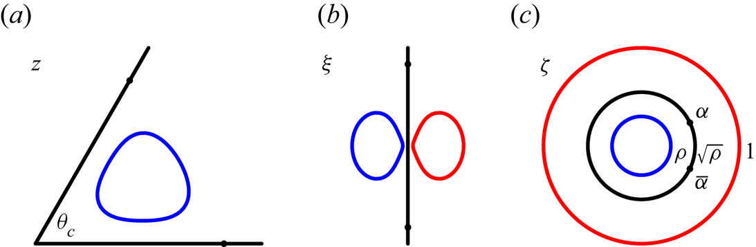
The standard conformal mapping approach for free-boundary value problems in inviscid flow that goes back to Michell (Reference Michell1890) is used to find the shape of the hollow vortex. Conformal maps are constructed between the corner, a half-plane and a concentric annulus as shown in figure 1. An image vortex in the non-physical portion of the half-plane allows the boundary condition of no normal flow on the solid walls to be satisfied. The boundaries of the hollow vortex and its image correspond to circles in the annulus.
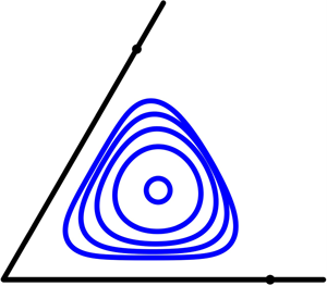
(a) The physical  $z$-plane with the corner; (b) the auxiliary
 $\xi$-plane; (c) the
 $\zeta$-plane containing the annulus, where
 $\rho$ is the radius of the inner circle of the annulus, and
 $\alpha$ and
 $\overline{\alpha}$ are the pre-images of the stagnation points along the corner boundary. (Here,
 $\rho =0.3$ and
 $\theta _{c}={\rm \pi} /3$; stagnation points along the wall are denoted by black circles.)

2. Problem formulation
A sketch of the physical domain is shown in figure 1(a). We consider flow inside a corner with interior angle  $\theta _{c}$. The fluid lies between a solid wall along positive
 $x$ and a solid wall making the angle
 $\theta _{c}$ with the positive real axis. We have
 $0 < \theta _{c} < 2{\rm \pi}$; the case
 $\theta _{c} = {\rm \pi}$ recovers the Pocklington dipole.
A hollow vortex is a steady-state constant-pressure region of finite area with non-zero circulation around it. The boundary of a hollow vortex is a streamline. For two-dimensional inviscid, incompressible, irrotational flow, Bernoulli's equation on the boundary gives
 \begin{equation} p + \frac{|\boldsymbol{u}|^2}{2} = \text{constant}, \end{equation}
where  $p$ is pressure and
 $\boldsymbol{u}$ is velocity. The pressure on the hollow vortex boundary is constant, and therefore Bernoulli's equation shows that the speed of the flow must be constant on the boundary as well. This shows that the boundary of a hollow vortex is a vortex sheet, and hollow vortices can be thought of as steady vortex sheets. As this is a two-dimensional incompressible and irrotational flow, the solution can be written in terms of a complex potential,
 $w$, with a corresponding complex velocity
 $\textrm {d} w/\textrm {d} z$.
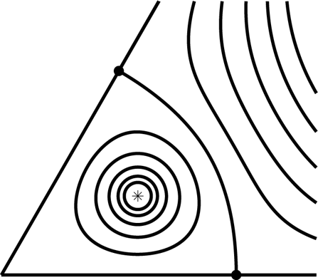
The flow describing a stationary point vortex in a corner gives insight into the hollow vortex solution because, as the area of a hollow vortex goes to zero, the point vortex flow field should be recovered. In particular, the flow for a hollow vortex in a corner is therefore expected to have the same number of stagnation points as a point vortex in a corner. Furthermore, the flow far away from the hollow vortex must be the same as the flow far away from the point vortex. Streamlines for a point vortex in equilibrium in a corner are shown in figure 2, where it can be seen that the flow has two stagnation points along the wall (for  $\theta_c < {\rm \pi}$, the flow velocity is also zero at the origin). Note that the flow is self-similar: one can rescale using the distance from the corner to the stagnation points as a unit of length, and then there is a unique flow.
Streamlines for a point vortex in equilibrium in a corner. The point vortex is denoted by an asterisk. The two stagnation points of the flow on the walls are denoted by filled circles. The speed of the flow is also zero at the origin.

The complex potential for a point vortex in a corner is found using conformal mapping and the method of images and is
 \begin{equation} w_{{pv}}(z) = \frac{\varGamma}{2{\rm \pi}\mathrm{i}} \left[\log{\left(z^{{\rm \pi}/\theta_{c}} - z_0^{{\rm \pi}/\theta_{c}}\right)} - \log{\left( z^{{\rm \pi}/\theta_{c}} - \overline{z_0}^{{\rm \pi}/\theta_{c}}\right)}\right] - S z^{{\rm \pi}/\theta_{c}}, \end{equation}
where  $S$ is a real number with the same sign as
 $\varGamma$ that describes the strength of the background generalized straining flow, and
 $z_0$ is the position of the vortex. The potential (2.2) behaves like
 $-S z^c$ for large
 $|z|$, where
 $c = {\rm \pi}/\theta _c$. This behaviour will also hold for the hollow vortex. The condition for the vortex to be stationary comes from requiring
 $\dot {z}_0 = 0$, where
 \begin{equation} \dot{\overline{z_0}} = \frac{\varGamma}{2{\rm \pi}\mathrm{i}} \left[ \frac{c-1}{2z_0} - \frac{c z_0^{c-1}}{z_0^c - \overline{z_0}^c} \right] - S c z_0^{c-1}. \end{equation}
The result is  $z_0 = (\mathrm {i}\varGamma /(4{\rm \pi} Sc))^{1/c}$, so that
 $z_0$ is along the bisector of the corner (when
 ${\rm \pi} = \theta _{c}$, the position parallel to the boundary is arbitrary and can be taken to be on the
 $y$-axis).
3. Conformal mapping
The solution for the hollow vortex is constructed using conformal maps between the three planes shown in figure 1. The physical  $z$-plane (figure 1a) is related to the
 $\xi$-plane (figure 1b) via
 \begin{equation} z = f(\xi) = (-\mathrm{i} \xi)^{\theta_{c}/{\rm \pi}}, \end{equation}
where  $\theta _{c}$ is the interior angle of the corner. The function
 $f(\xi )$ has a branch point at the origin, and its branch cut is taken to be in the right half-plane, i.e. outside the physical domain. The
 $\xi$-plane is essentially the same as the physical plane in Reference Crowdy, Llewellyn Smith and FreilichCLSF. An extension of the Riemann Mapping Theorem shows that any doubly connected domain can be mapped onto a concentric annulus. We take
 $g$ to be the unknown map from the circular annulus
 $\rho < |\zeta | < 1$ in the
 $\zeta$-plane (figure 1c) to the
 $\xi$-plane with the interiors of the vortex and of its unphysical image removed. The flow region will correspond to the region
 $\rho < |\zeta | < \beta$, where
 $\beta$ will be found. The map from the annulus to the corner is written as
 $h(\zeta ) = f(g(\zeta ))$.
In terms of the variable  $\zeta$, we write the complex potential describing the flow around the hollow vortex in the corner as
 $W(\zeta )$ and the complex velocity in the physical
 $z$-plane as
 $\textrm {d} w / \textrm {d} z = R(\zeta )$.
We require the map  $g$ to be one-to-one, and take the point at infinity in the
 $\xi$-plane to correspond to the simple pole
 $\beta$ in the
 $\zeta$-plane. Hence,
 \begin{equation} g(\zeta) = \frac{b}{\zeta - \beta} + \cdots \end{equation}
near  $\zeta = \beta$, where
 $b$ is chosen to be a positive real number. This means that the inner circle
 $|\zeta | = \rho$ maps to the image of the vortex boundary in the left half-plane in
 $\xi$, while the circle
 $|\zeta | = \beta$ maps to the imaginary axis in the
 $\xi$-plane. The outer circle
 $|\zeta | = 1$ maps to the reflection of the vortex boundary image about the imaginary
 $\xi$-axis, which is not in the physical domain.
From the above, we see that the complex potential  $W(\zeta )$ satisfies the following conditions. The kinematic boundary condition requires
 $\textrm{Im}\,W(\zeta )$ to be constant on the boundaries and on the vortex boundary. The circulation of the vortex, which is the change in the multivalued function
 $W(\zeta )$ around the vortex, is
 $\varGamma$. Large
 $|z|$ corresponds to large
 $|\xi |$, so that
 \begin{equation} W(\zeta) \sim -S z^{{\rm \pi}/\theta_{c}} = \mathrm{i} S \xi \sim \frac{\mathrm{i} S b}{\zeta - \beta} \end{equation}
near  $\zeta = \beta$.
In turn, the complex velocity,  $\textrm {d} w / \textrm {d} z = R(\zeta )$, satisfies the following conditions. From differentiating the asymptotic conditions of the complex potential in the physical plane, we have
 \begin{equation} R(\zeta) \sim -\frac{S {\rm \pi}}{\theta_{c}} \left(\frac{-\mathrm{i} b}{\zeta - \beta}\right)^{1-\theta_{c}/{\rm \pi}} \end{equation}
near  $\zeta = \beta$. The hollow vortex property of constant speed on the boundary from (2.1) means
 $|R(\zeta )|$ is constant on the vortex boundary. Finally,
 $R(\zeta ) = 0$ at the two stagnation points. The behaviour of
 $R(\zeta)$ near the origin depends on the angle: it vanishes for
 $0 < \theta _{c} < {\rm \pi}$, it is finite for
 $\theta _{c} = {\rm \pi}$, and it has an algebraic singularity for
 ${\rm \pi} < \theta _{c} < 2{\rm \pi}$.
We seek a hollow vortex that is symmetric about the real and imaginary axes in the  $\xi$-plane. These symmetries should persist in the
 $\zeta$-plane, and we now use them to determine which points in
 $\zeta$ correspond to the important points in
 $z$: the origin, infinity and the stagnation points.
In the  $\xi$-plane, the vortex boundaries are symmetric under reflection about the vertical axis. In the annulus, the boundaries are concentric circles, and mapping them onto each other is carried out by inversion. Hence, to retain the symmetry of the vortex, the vortex boundaries should be inverse circles about the image of the axis in the annulus. The boundary circles have radii
 $\rho$ and
 $1$, so the axis between the vortices in the
 $\xi$-plane must correspond to a circle with radius
 $\beta \equiv \sqrt {\rho }$ inside the annulus. The stagnation points are on this circle.
In the  $\xi$-plane, the vortex boundaries are also symmetric about the real axis which runs through the centroids of the vortices. From (3.1), we map the real
 $\xi$-axis to the real axis in the
 $\zeta$-plane. The images of the
 $\xi$-axes meet at
 $0$ and
 $\infty$, and these map to
 $-\beta$ and
 $\beta$, respectively, in the
 $\zeta$-plane. The two stagnation points on the walls are complex conjugates of each other in the annulus, so that we can write them as
 $\alpha$ and
 $\overline {\alpha }$ with
 $|\alpha |=\beta$.
4. Solution
4.1. Complex potential and complex velocity
The conformal mapping solution is constructed using the SK prime function. Schottky-Klein prime functions exists for higher connectivity domains (i.e. with larger genus). For genus  $2$, i.e. the annulus, the SK prime function can be written explicitly as (Crowdy Reference Crowdy2020)
 \begin{equation} \omega(\zeta,a) = (\zeta - a) \prod_{k=1}^\infty \frac{\left(1 - \rho^{2k} \zeta/a\right) \left(1- \rho^{2k} a/\zeta\right)}{\left(1-\rho^{2k}\right)}, \end{equation}
where  $\zeta$ lies inside the annulus,
 $0 \leq \rho \leq 1$, and
 $a$ can be any complex number. For the annulus, the following prime function identities hold:
 \begin{equation} \omega(\zeta,a) = -\zeta a \overline{\omega(1/\bar{\zeta},1/\overline{a})}, \quad \omega(\rho^2 \zeta,a) = -\frac{a}{\zeta} \omega(\zeta,a). \end{equation}
The conditions on the conformal map  $W(\zeta )$ characterize it as a map that takes circular vortex boundaries in
 $\zeta$ to horizontal lines in
 $W$. This type of map is called a parallel slit map, and can be written using the SK prime function as
 \begin{equation} \phi_{\theta}(\zeta,a) = \left( \frac{\partial }{\partial a} - \textrm{e}^{2\mathrm{i}\theta} \frac{\partial }{\partial \overline{a}} \right) \log{\left( \frac{\omega(\zeta,a)}{|a| \omega(\zeta,1/\overline{a})} \right)}. \end{equation}
The map  $\phi _{\theta }(\zeta ,a)$ takes concentric circles in the annulus to parallel lines making an angle
 $\theta$ with the real axis, with a simple pole at
 $\zeta = a$. This allows us to write the complex potential as
 \begin{equation} W(\zeta) = D \textrm{e}^{-\mathrm{i}\theta_p}\phi_{\theta_p}(\zeta,\beta) + \frac{\varGamma}{2 {\rm \pi}\mathrm{i}} \log{\zeta}. \end{equation}
The form of the parallel slit map ensures that  $W$ has constant imaginary part along the images of the vortex boundaries as long as
 $D$ is real and
 $\theta _p$ is
 ${\rm \pi} /2$. The logarithm term ensures the correct circulation. It does not affect the kinematic boundary condition, since the logarithmic term has constant imaginary part on constant
 $|\zeta |$. The potential (4.4) is the same as that in Reference Crowdy, Llewellyn Smith and FreilichCLSF and does not depend on the angle
 $\theta _{c}$. The relations between the notation used in Reference Crowdy, Llewellyn Smith and FreilichCLSF and that used here are discussed in appendix A.
Starting with the prime function product representation in (4.1) and carrying out the operations in the definition of a parallel slit map in (4.3), the parallel slit map for the present domain can be written as
 \begin{align} \phi_{\theta}(\zeta,a) &= -\frac{1}{\zeta - a} +\sum_{k=1}^{\infty} \left( \frac{\rho^{2k} \zeta}{a^2(1- \rho^{2k}\zeta/a)} - \frac{\rho^{2k}/\zeta}{1-\rho^{2k}a/\zeta} \right) + \frac{1}{2} \left( \frac{a \textrm{e}^{\mathrm{i} 2 \theta} - \overline{a}}{|a|^2} \right) \nonumber\\ &\quad +\, \frac{\textrm{e}^{\mathrm{i} 2 \theta}}{\overline{a}^2 (\zeta - 1/\overline{a})} - \frac{\textrm{e}^{\mathrm{i} 2\theta}}{\overline{a}^2}\sum_{k=1}^{\infty} \left( \frac{\overline{a}^2 \rho^{2k} \zeta}{1- \rho^{2k}\zeta \overline{a}} - \frac{\rho^{2k}/\zeta}{1-\rho^{2k}/(\zeta \overline{a})} \right), \end{align}
showing that  $\phi _{\theta }(\zeta ,a)$ has a simple pole with residue
 $-1$ at
 $\zeta = a$. Condition (3.3) then implies that
 \begin{equation} D = S b. \end{equation}
The constants  $S$ and
 $b$ are both real, and
 $\theta _p$ is
 ${\rm \pi} /2$. The zeros of
 $\textrm {d} w/\textrm {d} z$ are the same as those of
 $W'(\zeta )$. Hence,
 $W'(\alpha ) = 0$, which leads to a relationship between the constants of the problem, which is the same as (24) of Reference Crowdy, Llewellyn Smith and FreilichCLSF.
The condition of constant speed,  $|R(\zeta )|$, on the boundary of the vortex leads us to view
 $R(\zeta )$ as a conformal map that takes the circular vortex boundaries in
 $\zeta$ to circular arcs in
 $R$. This type of map is called a circular slit map, and can be written using the SK prime function as
 \begin{equation} w_{a}(\zeta) = \frac{\omega(\zeta,a)}{|a| \omega(\zeta,1/\overline{a})}, \end{equation}
which has a simple zero at  $\zeta =a$ and a simple pole outside the domain at
 $\zeta =1/\overline {a}$.
This allows us to write the complex velocity as
 \begin{equation} R(\zeta) = \frac{A}{\zeta} w_{\alpha}(\zeta) w_{\overline{\alpha}}(\zeta) \left( \frac{w_{-\beta}(\zeta)}{w_{\beta}(\zeta)} \right)^{1-\theta_{c}/{\rm \pi}}, \end{equation}
where  $A$ is a constant determined below. This function has zeros at the stagnation points and has the appropriate pole at
 $\zeta = \beta$ to satisfy the behaviour in (3.4). Any power of
 $\zeta$ can be considered as a circular slit map because
 $|\zeta |$ is constant along arcs of constant radius. The complex velocity
 $R(\zeta )$ is therefore a product of circular slit maps, since each individual circular slit map has constant magnitude on the circular boundaries of the domain. The inverse power of
 $\zeta$ in (4.8) ensures that the speed on the two boundaries in the
 $\xi$-plane is the same as in Reference Crowdy, Llewellyn Smith and FreilichCLSF; this is essentially the method of images. The branch cut is the same as discussed previously.
One can use the definition of the prime function in (4.1) to obtain an expression for  $A$ in terms of the other quantities from
 \begin{equation} R(\zeta) \sim \frac{A}{\beta} w_{\alpha}(\beta) w_{\overline{\alpha}}(\beta) \left( \frac{w_{-\beta}(\beta) \beta \omega(\beta,1/\beta)}{(\zeta - \beta) \prod_{k=1}^{\infty}{(1-\rho^{2k})}} \right)^{1-\theta_{c}/{\rm \pi}} \end{equation}
as  $\zeta \rightarrow \beta$. Using this in (3.4) gives
 \begin{equation} A = -\frac{S {\rm \pi}\beta^{\theta_{c}/{\rm \pi}}}{\theta_{c} w_{\alpha}(\beta) w_{\overline{\alpha}}(\beta) } \left(\frac{-\mathrm{i} a \prod_{k=1}^{\infty}{(1-\rho^{2k})}}{w_{-\beta}(\beta) \omega(\beta,1/\beta)}\right)^{1-\theta_{c}/{\rm \pi}}. \end{equation}
The details of this expression are not needed below, because there is still an arbitrary scaling in the solution that will be determined a posteriori. It is useful, however, to note the argument of  $A$ above in the numerical calculations.
4.2. Determining parameters
For each angle  $\theta _{c}$, we expect a one-parameter family of solutions parameterized by
 $\rho$. We require the map to be single-valued, which means that
 \begin{equation} \int_{C} \frac{\textrm{d} z}{\textrm{d} \zeta} \textrm{d} \zeta = 0, \end{equation}
where  $C$ is any closed loop in the domain. Note that the branch cuts lie outside the interior of the annulus with
 $\rho < |\zeta | < \beta$. We have
 \begin{equation} \frac{\textrm{d} z}{\textrm{d} \zeta} = \frac{\textrm{d} W/\textrm{d}\zeta}{R(\zeta)}, \end{equation}
where  $\textrm {d} W/\textrm {d}\zeta$ can be obtained explicitly from (4.4). This leads to the relation
 \begin{equation} z(\zeta) = \int_{-\beta}^\zeta \frac{\textrm{d} W / \textrm{d} \zeta'}{R(\zeta')}\,\textrm{d} \zeta'. \end{equation}
Given  $\rho$ and
 $\theta _{c}$, we solve (4.11) to obtain
 $\varTheta$, the argument of the stagnation point
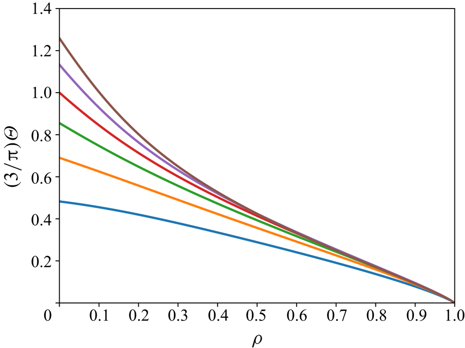
 $\alpha$, as in Reference Crowdy, Llewellyn Smith and FreilichCLSF. Results of
 $\varTheta$ for a variety of corner angles are shown in figure 3. In this and all subsequent figures, the values
 $\theta _{c} = {\rm \pi}/4$,
 ${\rm \pi} /2$,
 $3{\rm \pi} /2$,
 ${\rm \pi}$ (the Pocklington dipole),
 $5{\rm \pi} /4$ and
 $3{\rm \pi} /2$ are used. One can show that
 \begin{equation} \varTheta = \tan^{-1}{\frac{\sqrt{4\theta_{c}{\rm \pi}-\theta_{c}^2}}{2{\rm \pi}-\theta_{c}}} \end{equation}
for  $\rho = 0$. The integrand in (4.11) is independent of the constants
 $D$ and
 $A$.
Normalized stagnation point phase,  $3\varTheta /{\rm \pi}$, as a function of
 $\rho$ for
 $\theta _{c} = {\rm \pi}/4$,
 ${\rm \pi} /2$,
 $3{\rm \pi} /2$,
 ${\rm \pi}$,
 $5{\rm \pi} /4$ and
 $3{\rm \pi} /2$. Smaller values of
 $\theta _{c}$ correspond to smaller
 $\varTheta$.

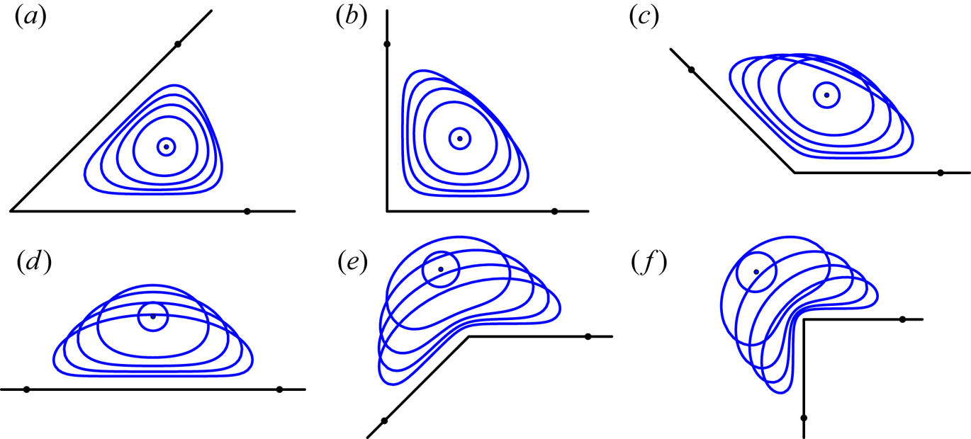
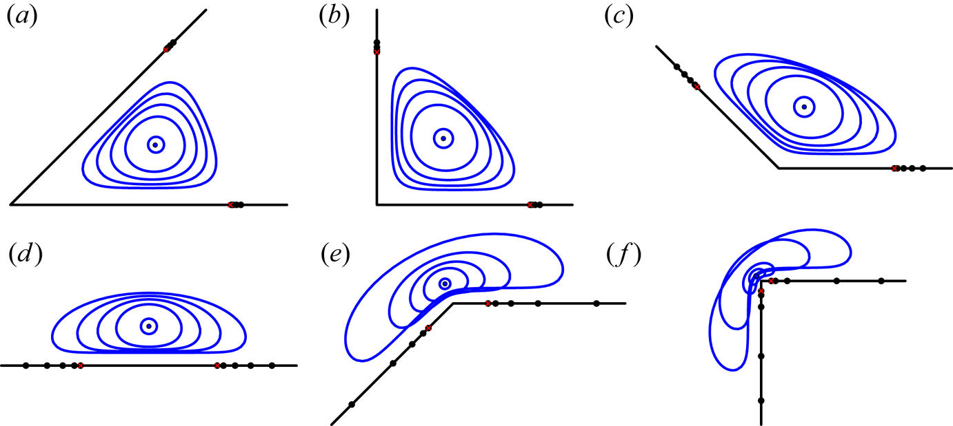
This calculation leaves an undetermined parameter. This can be used to set the overall scale of the vortex. We choose it so that  $|z(\alpha )|=1$, so that the distance to the stagnation points is unity. Alternatively, we can take the distance of the centroid of the vortex to the corner to be the unit of distance. As a result, the plots of vortex boundaries in figures 4, 5 and 6 do not have axes.
The five vortices in each corner correspond to five equally spaced values of  $\rho$ in
 $0.01 \le \rho \le 0.5$. Each vortex is scaled individually so that the stagnation points are at distance unity from the corner.

As for figure 4, but normalized so that the geometric centroid is at distance unity from the corner. The stagnation points of the point vortex are in red.

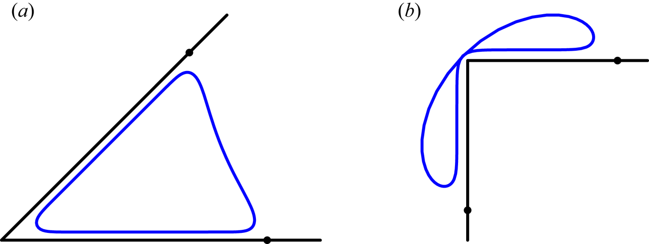
(a) For  $\theta _{c} \le {\rm \pi}$ and large
 $\rho$, the vortex conforms to the shape of the corner boundary. Here,
 $\theta _{c}={\rm \pi} /4$ and
 $\rho =0.8$. (b) For
 $\theta _{c} > {\rm \pi}$ and large
 $\rho$, the vortex boundary can become tangent to itself, which is unphysical because the speed is constant along the boundary and would therefore have two different values at the tangency point. Here,
 $\rho =0.64$ and
 $\theta _{c}=3{\rm \pi} /2$.

Once the condition (4.11) has been enforced, the boundary of the hollow vortex is found by evaluating (4.13) along the circle  $|\zeta | = \rho$. We first integrated from
 $-\beta$ to
 $-\rho$ to move from the corner to the closest point of the vortex to the corner (which is along the bisector of the angle by symmetry). This integrand has an algebraic singularity at
 $\zeta = -\beta$, since
 $R(\zeta )$ is singular at a corner with
 ${\rm \pi} < \theta _{c} < 2{\rm \pi}$. The integral, however, can be carried out numerically with no trouble.
5. Results
Figure 4 shows the boundaries of a number of stationary hollow vortex solutions for different values of  $\rho$ and different angles. The hollow vortices in each plot have been individually normalized so that the stagnation points are the same for all vortices. Figure 5 shows the same solutions normalized so that their centroids are at unit distance from the corner. The point vortex solution is plotted as a filled circle in each figure. As
 $\rho \rightarrow 0$, the hollow vortex boundary shrinks to the point vortex, as expected. For
 $\theta _{c} > {\rm \pi}$, the vortex boundary intersects itself for large enough
 $\rho$, as shown in figure 6(b). This is similar to what happens for the hollow vortex in strain examined by Llewellyn Smith & Crowdy (Reference Llewellyn Smith and Crowdy2012), which self-intersects if the strain is too large.
6. Discussion
As shown in figure 6(b), we find numerically that, as  $\rho$ increases for
 $\theta _c > {\rm \pi}$, the vortex boundary ends up being tangent to itself at a point along the bisector of the corner, by symmetry. This solution is not physically acceptable. It is possible to find the corresponding critical value
 $\rho _c$ numerically, and as
 $\theta _c$ increases,
 $\rho _c$ decreases. One can find further solutions for
 $\rho > \rho _c$; these self-intersecting solutions are not physically acceptable either. Presumably another solution family branches off at the critical value of
 $\rho _c$, with the solution beyond it consisting of two symmetric vortices with near-cusps. Finding it will be difficult, since the flow domain now has genus
 $2$, which requires a completely different analysis.
Figure 6(a) shows that as  $\rho \to 1$ for
 $\theta _c < {\rm \pi}$, the vortex starts to conform to the shape of boundaries and take the shape of a curvilinear triangle. While there do not seem to be any discussions in the literature of the asymptotics of the prime function as
 $\rho \to 1$, we see physically that the solution takes the form of two narrow flows of constant velocity along the boundary, connected by a stagnation point flow near the apex of the corner, with the outer side slightly curved. The velocity profile in the jets is parallel to the boundary and uniform, and the speed is just the speed of the fluid on the vortex boundary, which is given exactly by
 $q_0 = |A| \rho ^{-1}$. The width of the jet
 $d$ can be obtained from the relation
 $2q_0 d = -Sa \beta ^{-1} (1 + \mu \log {\rho })$, resulting from the difference in streamfunction between the two vortices. We find numerically that
 $\mu = m (1-\rho )^{-1}$ as
 $\rho \to 1$ with
 $m$ depending on
 $\theta _c$, but the form of
 $m$ does not seem to be available from analysis. We are hence led to the leading-order result
 \begin{equation} d \sim -\frac{S a \sqrt{\rho}}{2 |A|} \left( 1 + \frac{m \log{\rho}}{1-\rho} \right). \end{equation}
We have only examined symmetric solutions, as in CSLF. We do have some evidence that no asymmetric solution exists in this problem: if one can be found in the same form as above, but with asymmetric stagnation points on the circle  $|\zeta | = \beta$, then the condition that
 $W'(\zeta )$ vanishes at the stagnation points becomes four equations in two unknowns and is found numerically to have no solution except for the symmetric case. This is not a fully rigorous proof, however.
One could also generalize to multiple vortices along the bisector of the angle. A counting argument shows that this configuration has (multiple) solutions in the point vortex case, and then an approach, such as that in Llewellyn Smith (Reference Llewellyn Smith2014), indicates that desingularized versions will exist. Finding them numerically will be a challenge, requiring higher-genus SK functions.
The stability of the family of vortices could be examined using the same approach as in Reference Crowdy, Llewellyn Smith and FreilichCLSF. The non-dimensional growth rate is  $\sigma = \lambda \varGamma /(2{\rm \pi} q_0^2)$, where
 $\lambda$ is the dimensional growth rate. The general stability problem combines stability of the interface shape and stability associated with displacements of the centroid. In the point vortex limit, one finds
 $\sigma \sim \lambda \rho d^2/\varGamma$ (up to multiplicative factors), where
 $d$ is the distance to the point vortex. Hence, the spectrum of neutral modes found in Reference Crowdy, Llewellyn Smith and FreilichCLSF has high dimensional frequency when expressed in terms of variables relevant to the point vortex pair. This is consistent with the fact that in the point vortex limit the equilibrium solution obtained from (2.3) is neutrally stable with non-zero frequency for
 $\theta _c < {\rm \pi}$, has zero growth rate for
 $\theta _c = {\rm \pi}$ and is unstable for
 $\theta _c > {\rm \pi}$ (this does not appear to have been mentioned in the literature). Hence, for
 $\theta _c > {\rm \pi}$ the system is unstable for arbitrary small
 $\rho$, and there is not much sense examining it for general
 $\rho$. As
 $\rho$ increases, one can no longer separate displacement and shape instability. The stability problem is formulated in the complex
 $w$-plane, in which the vortex takes a simple shape, which is then transformed to the
 $\zeta$-plane. An important difference is that there is now only one vortex, along with a solid boundary at
 $|\zeta | = \beta$, at which, in the notation of Reference Crowdy, Llewellyn Smith and FreilichCLSF,
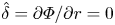 $\hat {\delta } = \partial \varPhi /\partial r = 0$, where
 $\hat {\delta }$ and
 $\Phi$ now designate the streamfunction and potential perturbations, respectively, along the solid boundary, while
 $r$ is the radial distance in the
 $\zeta$-plane. We do not pursue the calculation further. It now contains
 $\theta _c$-dependence, and preliminary indications suggest that as
 $\theta _c$ approaches
 $0$ or
 ${\rm \pi}$, the calculations become numerically delicate. Away from this range, one can find a critical instability threshold
 $\rho _c(\theta _c)$, with indications of multiple bubbles of instability (typical of Hamiltonian stability problems) in the system. The current stability problem, which has one free surface and one solid boundary, seems to have fewer degrees of freedom than that of Reference Crowdy, Llewellyn Smith and FreilichCLSF; the values obtained for
 $\rho _c$ do seem larger, of the order of
 $0.08$–
 $0.12$. More work is required to understand the stability problem fully.
7. Conclusion
A stationary hollow vortex surrounded by irrotational flow has been found inside a wedge of fluid bounded by a corner of arbitrary angle using a conformal mapping approach. This is the first combined use of the SK prime function with algebraic functions to the authors’ knowledge. For special values of  $\theta _{c}$, namely divisors of
 ${\rm \pi}$ such as
 ${\rm \pi} /2$,
 ${\rm \pi} /3$,
 ${\rm \pi} /4$ and so on, it should be possible to construct the solution using higher-genus SK prime functions and symmetries. The algebra would rapidly become unmanageable, although presumably the final form of the solution would lead to identities between SK functions of different genus.
The problem of a steady vortex patch in a corner does not seem to have been investigated in detail, although the propagating vortex patch dipole has been examined (Deem & Zabusky Reference Deem and Zabusky1978; Pierrehumbert Reference Pierrehumbert1980; Saffman & Tanveer Reference Saffman and Tanveer1982). The Sadovskii dipole (or patch sheet), a vortex patch bounded by a vortex sheet, is a generalization of both Sadovskii (Reference Sadovskii1971) and Tanveer (Reference Tanveer1986). Similarly, one could examine patch sheet equilibria in a corner.
Perturbing the point vortex equilibrium with potential (2.2) leads to periodic motion for  $\theta _{c} < {\rm \pi}$. The general case of a point vortex in a right-angle corner was investigated by Suh (Reference Suh1993), and its transport properties provide an interesting model problem for non-periodic transport (authors' unpublished observations). The case of the point vortex in the corner could be examined similarly. For the hollow vortex, the problem is much more difficult, since the vortex sheet would evolve and would have to be obtained using a numerical approach similar to those used for water waves (e.g. Vanden-Broeck Reference Vanden-Broeck2010; Baker & Xie Reference Baker and Xie2011).
Acknowledgements
This work was inspired by lectures given by Darren Crowdy during the NSF-CBMS Conference on Solving Problems in Multiply Connected Domains in 2018. The conference was supported by NSF award DMS-1743920 (Co-PIs Bernard Deconinck, Stefan Llewellyn Smith and Tom Trogdon) and the Department of Mathematics at the University of California, Irvine. Conversations with Ted Johnson were also helpful, as were comments from the referees. This research was partly supported by NSF award DMS-1522675. S.G.L.S. was also partly supported by NSF award CBET-1706934.
Declaration of interests
The authors report no conflict of interests.
Appendix A. Formulation using  $P$, $K$ and $L$


For ease of comparison with Reference Crowdy, Llewellyn Smith and FreilichCLSF, we provide here the relevant formulas in terms of the definitions of the SK functions used in that work. For the annulus, the SK prime function and required related functions are defined by
 \begin{equation} P(\zeta,\rho) = (1 - \zeta) \prod_{k=1}^\infty \left(1 - \rho^{2k}\zeta\right) \left(1 - \rho^{2k}\zeta^{-1}\right) = - a^{-1} \prod_{k=1}^{\infty} \left( 1-\rho^{2k}\right) \omega{(a\zeta,a)}, \end{equation}
and
 \begin{equation} K(\zeta,\rho) = \frac{\zeta P'(\zeta,\rho)}{P(\zeta,\rho)}, \quad L(\zeta,\rho) = \zeta K'(\zeta,\rho). \end{equation}
Primes indicate derivatives with respect to  $\zeta$. Below we will suppress the
 $\rho$ in the argument list. Then
 \begin{equation} W(\zeta) = \frac{\mathrm{i} Sb}{\beta} \left[ K(\zeta/\beta) + K(\zeta\beta) \right] + \frac{\varGamma}{2 {\rm \pi}\mathrm{i}} \log{\zeta} = \frac{\mathrm{i} Sb}{\beta} \left[ K(\zeta/\beta) + K(\zeta\beta) - \mu \log{\zeta} \right], \end{equation}
which is formally the same (with  $U$ replaced by
 $S$ and
 $a$ replaced by
 $b$) as in Reference Crowdy, Llewellyn Smith and FreilichCLSF, and
 \begin{equation} R(\zeta) = \frac{A}{\zeta} \frac{P(\zeta/\alpha)P(\zeta/\overline{\alpha})}{P(\zeta\overline{\alpha})P(\zeta\alpha)} \left( \frac{P(-\zeta/\beta)P(\zeta\beta)}{P(-\zeta\beta)P(\zeta/\beta)} \right)^{1-\theta_{c}/{\rm \pi}}, \end{equation}
where we have used the fact that  $\beta$ is real. Equation (24) of Reference Crowdy, Llewellyn Smith and FreilichCLSF is
 \begin{equation} L(\textrm{e}^{\mathrm{i}\varTheta}) + L(\rho\textrm{e}^{\mathrm{i}\varTheta}) = \mu. \end{equation}