
1. Introduction
Self-propelled organisms swimming in confined geometries have attracted considerable attention due to their relevance in the fertilization process (Miki & Clapham Reference Miki and Clapham2013), microalgae cultivation (Posten Reference Posten2009; Oncel & Kose Reference Oncel and Kose2014), bio-remediation (Suresh Kumar et al. Reference Suresh Kumar, Dahms, Won, Lee and Shin2015) and evolutionary and ecological processes (Isard, Isard & Gage Reference Isard, Isard and Gage2001). The swimming of aquatic swimmers with sizes ranging from a few microns to several metres can fall into the finite inertial flow regime (Childress Reference Childress1981; Beckett Reference Beckett1986). The Reynolds number, Re = ρUL/μ, represents the ratio of inertial to viscous forces within the fluid, where ρ, μ, U and L are respectively the fluid density, the viscosity and the characteristic speed and length of the flow. For example, Re ranges 0.1–1 for freely swimming zooplankton Daphnis magna (Wickramarathna, Noss & Lorke Reference Wickramarathna, Noss and Lorke2014), 0.2–2 for Paramecia depending on whether it is in swimming or escaping mode (Ishikawa & Hota Reference Ishikawa and Hota2006), O(10) for Pleurobrachia and O(20–150) for copepods (Kiørboe, Jiang & Colin Reference Kiørboe, Jiang and Colin2010). The corresponding flow problems require the Navier–Stokes (NS) equations to be solved in full.
The spherical squirmer model, one of the most famous mathematical microswimmer models first proposed by Lighthill (Reference Lighthill1952) and extended by Blake (Reference Blake1971), is widely adopted to mimic the self-propulsion produced by the coordinated motion of a dense array of cilia on the surface of the body. The model was initially proposed for considering the self-propelling of ciliates and microalgae, such as Opalina and Volvox, and well reproduces the flow field generated by Volvox swimming (Pedley, Brumley & Goldstein Reference Pedley, Brumley and Goldstein2016). It was used at first to simulate the nutrient uptake by self-propelled organisms (Magar, Goto & Pedley Reference Magar, Goto and Pedley2003; Magar & Pedley Reference Magar and Pedley2005). Subsequently, the squirmer model has been used to analyse swimming efficiency (Michelin & Lauga Reference Michelin and Lauga2010, Reference Michelin and Lauga2013), hydrodynamic interactions with a wall (Ishimoto & Gaffney Reference Ishimoto and Gaffney2013; Ouyang, Lin & Ku Reference Ouyang, Lin and Ku2018a), two-body hydrodynamic interactions (Ishikawa, Simmonds & Pedley Reference Ishikawa, Simmonds and Pedley2006; Götze & Gompper Reference Götze and Gompper2010; Navarro & Pagonabarraga Reference Navarro and Pagonabarraga2010; Ouyang, Lin & Ku Reference Ouyang, Lin and Ku2019), rheology of suspensions (Ishikawa & Pedley Reference Ishikawa and Pedley2007), mixing by swimmers (Thiffeault & Childress Reference Thiffeault and Childress2010) and collective swimming (Ishikawa & Pedley Reference Ishikawa and Pedley2008; Ishikawa, Locsei & Pedley Reference Ishikawa, Locsei and Pedley2008; Zöttl & Stark Reference Zöttl and Stark2014; Lin & Gao Reference Lin and Gao2019). Many of the efforts in tube flow have been made in the limit of Stokes flow, i.e. Re = 0. Zhu, Lauga & Brandt (Reference Zhu, Lauga and Brandt2013) have investigated the hydrodynamic behaviours and the propulsive efficiency of a squirmer inside a capillary tube using a boundary element method (BEM – the problem is linear at Re = 0). They find the rate of work necessary for swimming is increased by the confinement, and the puller (a squirmer propelled from the front) always displays stable locomotion at a location that depends on the strength of its force dipoles, whereas the pusher (a squirmer propelled from the rear) is unstable and ends up crashing into the walls of the tube. Zöttl & Stark (Reference Zöttl and Stark2012) studied the nonlinear dynamics of a squirmer in cylindrical Poiseuille flow analytically and compared with their numerical results obtained using multiparticle collision dynamics. They found the hydrodynamic interactions between the swimmer and confining channel walls lead to a dissipative dynamics and result in stable trajectories, which are different for pullers and pushers. Inspired by these two studies, we extend the swimming at a finite Re, mainly because organisms swim at a finite Re, and the inertia of the fluid has a significant impact on their swimming (Wang & Ardekani Reference Wang and Ardekani2012; Khair & Chisholm Reference Khair and Chisholm2014; Chisholm et al. Reference Chisholm, Legendre, Lauga and Khair2016; Li, Ostace & Ardekani Reference Li, Ostace and Ardekani2016; Ouyang et al. Reference Ouyang, Lin and Ku2018a, Reference Ouyang, Lin and Ku2018b; More & Ardekani Reference More and Ardekani2020). Wang and Ardekani (Reference Wang and Ardekani2012) first investigated a squirmer at a finite Re analytically and found that the inertia of the fluid enhances (hinders) the swimming speed of a pusher (puller) swimmer. Subsequently, Khair & Chisholm (Reference Khair and Chisholm2014) employed matched asymptotic expansion to calculate the swimming velocity of the squirmer through O(Re 2) and obtained approximations to the velocity and vorticity fields around the squirmer. With further increasing Re, numerical methods are utilized. Chisholm et al. (Reference Chisholm, Legendre, Lauga and Khair2016) employed a spectral element method and a finite volume method to investigate a squirmer across Re (0.01–1000), showing that the inertia results in significant divergences in the locomotion of a squirmer, where the swimming speed of a pusher increases with Re. In contrast, the swimming speed of a puller varies non-monotonically with Re. They also found that a pusher remains stable up to Re = 1000 due to the steady axisymmetric flow around the body, in contrast to a puller which becomes unstable due to the fact that the flow around the body becomes three-dimensional at a critical Re (that depends on the swimming modes). Similar behaviours are observed for a two-dimensional squirmer swimming in a power-law fluid (Ouyang et al. Reference Ouyang, Lin and Ku2018b). Subsequently, More & Ardekani (Reference More and Ardekani2020) investigate an inertial squirmer in a density stratified and infinite fluid with Re between 5 and 100, and Froude numbers (Fr) between 1 and 10. They find that increasing the fluid stratification strength reduces both pushers’ and pullers’ swimming speeds, compared with their speeds in a homogeneous fluid. The hydrodynamic interaction between a pair of inertial squirmers has been investigated recently (Li et al. Reference Li, Ostace and Ardekani2016), with results showing that the inertial effects change the contact time and dispersion dynamics of a pair of pusher swimmers and trigger hydrodynamic attraction for two pullers. Recently, Lin & Gao (Reference Lin and Gao2019) investigated the dynamics of inertial squirmers confined in a monolayer, showing that the inertia effect tends to suppress the dynamics with increasing Re. The investigation on an inertial squirmer in a tube is not complete as we still know little about the effects of the tube walls on the motion of an individual squirmer at finite Re.
Apart from a spherical squirmer, a squirmer dumbbell assembled by two squirmers has also attracted the attention of researchers since it is a minimal model of linked microswimmers and forms the basis for constructing more complex assemblies such as autonomous micro-robots (Ishikawa, Reference Ishikawa2019) and new functional soft materials (Cates & MacKintosh Reference Cates and MacKintosh2011; Winkler & Gompper Reference Winkler and Gompper2020). Recently, Ishikawa (Reference Ishikawa2019) has studied the stability of a squirmer dumbbell swimming in a bulk fluid. His results show that a dumbbell squirmer could not achieve a stable forward swimming in the far field without an external torque, and when the aft squirmer is a strong pusher, fore and aft swimming is stable, and swimming speed increases significantly. Clopés, Gompper & Winkler (Reference Clopés, Gompper and Winkler2020) have studied the swimming behaviour of a squirmer dumbbell using the multiparticle collision dynamics method. They find that pairs of strong pullers exhibit orders of magnitude smaller swimming efficiency than pairs of pushers, and pullers are preferentially aligned in an anti-parallel manner along the bond vector. In contrast, pushers are preferentially aligned normal to the bond vector with a specified relative angle at weak active stress.
This paper employs a direct-forcing fictitious domain method (DF-FDM) to simulate the spherical and dumbbell microswimmers swimming inside a tube. It aims to elucidate how the dumbbell shape and the tube constraint affect the hydrodynamics of the inertial microswimmers. The remainder of this paper is organized as follows. In $ 2, the DF-FDM and the squirmer and squirmer dumbbell model are outlined in detail. In $ 3, the numerical method is validated by performing the simulations for the motion of a squirmer in a capillary tube at extremely low Re, and in an infinite fluid field at finite Re. In $ 4, the results, including the swimming speeds, the far-field velocity, the swimming stability, the swimming power and the hydrodynamic efficiency for both the squirmers and the squirmer dumbbells, are presented and discussed. Finally, some concluding remarks are stated in $ 5.
2. Governing equations and numerical scheme
This section addresses the governing equations and the numerical method employed to simulate the locomotion of a squirmer and squirmer dumbbell through a Newtonian fluid at a finite Re. The fluid flow is governed by the incompressible Navier–Stokes equations in the entire computational domain,  $\varOmega$
 \begin{gather}{\rho _f}\frac{{\textrm{D}\boldsymbol{u}}}{{\textrm{D}t}} = \boldsymbol{\nabla }\boldsymbol{\cdot }\boldsymbol{\sigma },\quad \textrm{in}\;\varOmega ,\end{gather}
 \begin{gather}\boldsymbol{\nabla }\boldsymbol{\cdot }\boldsymbol{u} = 0,\quad \textrm{in}\;\varOmega ,\end{gather}
where D/Dt = ∂u/∂t + u⋅∇u is the material derivative, and ρf, u and σ are the fluid density, the fluid velocity and the fluid stress, respectively. For a rigid particle in the fluid, its motion is governed by Newton's equations,
 \begin{gather}M\frac{{\textrm{d}\boldsymbol{U}}}{{\textrm{d}t}} = {\boldsymbol{F}^H} + \left( {1 - \frac{1}{{{\rho_r}}}} \right)M\boldsymbol{g},\end{gather}
 \begin{gather}\frac{{\textrm{d(}\boldsymbol{J}\boldsymbol{\cdot }{\boldsymbol{\omega }_s})}}{{\textrm{d}t}} = {\boldsymbol{T}^H},\end{gather}
where M, J, U and ωs are, respectively, the particle's mass, its moment of inertia tensor, its translational velocity and its angular velocity; g is the gravitational acceleration, and ρr is the solid–fluid density ratio. Also, FH and TH are the hydrodynamic force and torque on the particle, respectively, which are defined by,
 \begin{gather}{\boldsymbol{F}^H}\textrm{ = }\int_{\partial S} {\boldsymbol{n}\boldsymbol{\cdot }\boldsymbol{\sigma }\,\textrm{d}S} ,\end{gather}
 \begin{gather}{\boldsymbol{T}^H}\textrm{ = }\int_{\partial S} {\boldsymbol{r} \times (\boldsymbol{n}\boldsymbol{\cdot }\boldsymbol{\sigma })\,\textrm{d}S} ,\end{gather}
where n is the unit outward normal on the solid particle surface S, and r is the position vector concerning the particle' centre.
The fictitious domain method for the interface-resolved simulations of particle-laden flows, initially proposed by Glowinski et al. (Reference Glowinski, Pan, Hesla and Joseph1999), fills the interior of the particle with the fluid, and a pseudo-body force is introduced over the particle's inner domain to enforce the fictitious fluid to satisfy the rigid-body motion constraint, leading to the following equations with interior of the particle body force:
 \begin{gather}{\rho _f}\frac{{\textrm{D}\boldsymbol{u}}}{{\textrm{D}t}} = \boldsymbol{\nabla }\boldsymbol{\cdot }\boldsymbol{\sigma }\textrm{ + }\boldsymbol{\lambda },\quad \textrm{in}\;{P_0}(t),\end{gather}
 \begin{gather}\boldsymbol{u} = \boldsymbol{U} + {\boldsymbol{\omega }_s} \times \boldsymbol{r} + {\boldsymbol{u}_s},\end{gather}
where λ is the pseudo-body force defined in the solid particle domain P 0(t) (Lagrange multiplier). Note that (2.7) originates from (2.1) by considering the pseudo-body force, and (2.8) describes a rigid motion of the fluid filling the particle fictitious domain. A DF-FDM proposed by Yu & Shao (Reference Yu and Shao2007) is employed here to cope with hydrodynamical interactions between the solid particle and the fluid. Note that us denotes a given velocity distribution introduced for the self-propelling problem.
In the present study, we use the squirmer model, a progressive waving envelope introduced to mimic both radial and angular oscillations on the boundary of a micro-swimmer with arrays of cilium-like Volvox (Pedley et al. Reference Pedley, Brumley and Goldstein2016). This swimming model has a reduced-order form considering a tangential velocity implemented on the boundaries of the body (in the frame of reference moving with the body); it reads
 \begin{equation}u_\theta ^s(\theta ) = {B_1}\;\textrm{sin}\;\theta + {B_2}\;\textrm{sin}\;\theta \;\textrm{cos}\;\theta ,\end{equation}
where θ is the angle concerning the swimming direction, and B 1 and B 2 are the first two squirming modes. The mode of the squirmer can hence be defined as a puller (β > 0), pusher (β < 0) or neutral squirmer (β = 0) according to the value of β = B 2/B 1 (B 1 > 0) (Ishikawa & Pedley Reference Ishikawa and Pedley2007). Pullers, such as Chlamydomonas, generate thrust from the front by using a breast-stroke-like motion. Pushers, on the contrary, generate thrust from the rear by propelling themselves by rearward-facing flagella, as in the case of Escherichia coli (Chisholm et al. Reference Chisholm, Legendre, Lauga and Khair2016). In the Stokes flow regime, the velocity of a squirmer in an infinite domain is U 0 = 2B 1/3 (Lighthill Reference Lighthill1952); hence, we adopt it as the velocity scale in this study. Even though this model is originally based on the swimming of swimmers in the Stokes flow limit, researchers have extended this reduced-order squirmer model to study the effects of inertia on the locomotion of swimmers in a variety of flow conditions (Wang & Ardekani Reference Wang and Ardekani2012; Zöttl & Stark Reference Zöttl and Stark2012; Zhu et al. Reference Zhu, Lauga and Brandt2013; Khair & Chisholm Reference Khair and Chisholm2014; Chisholm et al. Reference Chisholm, Legendre, Lauga and Khair2016; Li et al. Reference Li, Ostace and Ardekani2016; Lin & Gao Reference Lin and Gao2019; More & Ardekani Reference More and Ardekani2020).
In the framework of FDM, (2.9) is imposed on the squirmer surface by setting the following divergence-free velocity field inside the squirmer (Li et al. Reference Li, Ostace and Ardekani2016; Lin & Gao Reference Lin and Gao2019; More & Ardekani Reference More and Ardekani2020):
 \begin{align}{\boldsymbol{u}_s} &=
\left[ {{{\left( {\frac{r}{a}} \right)}^m} - {{\left(
{\frac{r}{a}} \right)}^{m + 1}}} \right]\left(
{u_\theta^s\;\textrm{cot}\;\theta +
\frac{{\textrm{d}u_\theta^s}}{{\textrm{d}\theta }}}
\right){\boldsymbol{e}_r}\nonumber\\ &\quad + \left[ {(m + 3){{\left(
{\frac{r}{a}} \right)}^{m + 1}} - (m + 2){{\left(
{\frac{r}{a}} \right)}^m}} \right]u_\theta
^s{\boldsymbol{e}_\theta
},\end{align}
where a is the radius of the squirmer, r is the distance from the squirmer's centre, er and eθ are, respectively, the unit vectors along the radial and polar directions and m is an arbitrary positive integer.
Integrating (2.7) and r × (2.7) over the solid particle interior and substituting into (2.5) and (2.6) yields
 \begin{gather}{\boldsymbol{F}^H}\textrm{ = } - \int_{{P_0}} {\boldsymbol{\lambda }\,\textrm{d}\kern0.06em \boldsymbol{x}} + \frac{M}{{{\rho _r}}}\frac{{\textrm{d}\boldsymbol{U}}}{{\textrm{d}t}} + \int_{{P_0}} {{\rho _f}\frac{{\textrm{d}{\boldsymbol{u}_s}}}{{\textrm{d}t}}\,\textrm{d}\kern0.06em \boldsymbol{x}} ,\end{gather}
 \begin{gather}{\boldsymbol{T}^H}\textrm{ = } - \int_{{P_0}} {\boldsymbol{r} \times \boldsymbol{\lambda }\,\textrm{d}\kern0.06em \boldsymbol{x}} + \frac{1}{{{\rho _r}}}\frac{{\textrm{d}(\boldsymbol{J}\boldsymbol{\cdot }{\boldsymbol{\omega }_s})}}{{\textrm{d}t}} + \int_{{P_0}} {{\rho _f}\left( {\boldsymbol{r} \times \frac{{\textrm{d}{\boldsymbol{u}_s}}}{{\textrm{d}t}}} \right)\textrm{d}\kern0.06em \boldsymbol{x}} .\end{gather}
The imposed active velocity does not generate a net force or torque, and on substituting (1.11) into (1.5) and (1.12) into (1.6), respectively, we obtain
 \begin{gather}\left( {\textrm{1} - \frac{1}{{{\rho_r}}}} \right)M\left( {\frac{{\textrm{d}\boldsymbol{U}}}{{\textrm{d}t}} - \boldsymbol{g}} \right)\textrm{ = } - \int_{{P_0}} {\boldsymbol{\lambda }\,\textrm{d}\kern0.06em \boldsymbol{x}} ,\end{gather}
 \begin{gather}\left( {\textrm{1} - \frac{1}{{{\rho_r}}}} \right)\frac{{\textrm{d}(\boldsymbol{J}\boldsymbol{\cdot }{\boldsymbol{\omega }_s})}}{{\textrm{d}t}}\textrm{ = } - \int_{{P_0}} {\boldsymbol{r} \times \boldsymbol{\lambda }\,\textrm{d}\kern0.06em \boldsymbol{x}} .\end{gather}
We employ a standard fractional step procedure for the fluid sub-problem to solve the above Navier–Stokes equation system in a fixed Eulerian domain with a uniform grid size Δx. A second-order half-staggered finite difference scheme is used for spatial discretization. One can refer to the work of Lin & Gao (Reference Lin and Gao2019) for more details of the squirmer dynamics employing the DF-FDM.
In a similar manner, the squirmer dumbbells are assembled by two identical squirmers arranged in tandem with their orientations in the direction of the arrow, as shown in figure 1, and are classified into puller (β > 0), pusher (β < 0) and neutral (β = 0) squirmer dumbbells. In this study, we assume that a rigid rod connecting the two squirmers is a phantom, and the two squirmers can only rotate around the mass centre O, as shown in figure 1. The distance between the two squirmers ds is an adjustable parameter used to form different squirmer dumbbells. Equations (2.13) and (2.14) govern the locomotion of a squirmer dumbbell. The main difference in the hydrodynamics of an individual squirmer and a squirmer dumbbell is that the individual squirmer of the dumbbell suffers non-zero forces and torques at a finite Re due to the breaking of the fore-and-aft symmetrical flow around it (whereas there is no net force or torque for the whole squirmer dumbbell).
Schematic of a squirmer dumbbell inside a tube. The squirmer dumbbell is assembled by two squirmers arranged in tandem with their orientations in the direction of the green arrow.

3. Validation
The DF-FDM has been shown to be accurate in simulating the motion of an individual squirmer and the hydrodynamical interactions between two identical squirmers (Lin & Gao Reference Lin and Gao2019). In this section, we perform the validations for the motion of a squirmer in a capillary tube at extremely low Re and in an infinite fluid field at a finite Re. These two validations are relevant to the present study for considering both the effect of the walls and the inertia on the squirmer dynamics. We simulate a swimming squirmer inside an infinitely long tube filled with a quiescent fluid to validate the effect of the tube walls on its speed. We initialize the squirmer at the centre of the tube with its orientation directing along the z-axis, and its velocity reaches a steady state after the initial transient dynamics. Note that we restrict the squirmer's translation and rotation to the x- and y-axes to better compare the speeds if not otherwise specified. Hence, the swimming speed U here denotes the velocity component of the squirmer in the z-axis. As Zhu et al. (Reference Zhu, Lauga and Brandt2013) have reported that the convergence criteria are satisfied with L = 3 ${\rm \pi}$R, in this study, the length L of the tube is set at 18R (R is the radius of the tube) to maintain convergence. We use periodic boundary conditions for the velocity in the z-direction. The moving mesh technology, shifting the flow field and the particle position one mesh distance once the particle moves a horizontal position that is greater than the centre of the domain in the horizontal direction (z-axis), is employed to keep the squirmer nearly at the centre of the calculated domain. A mesh size with 32 grid points across the diameter of the squirmer and a time step Δt less than 0.002 have been shown to be convergent (Lin & Gao Reference Lin and Gao2019) and are adopted here. As shown in figure 2, the speed of the squirmer inside the tube with the blocking ratio κ = 0.5 (κ = a/R) at Re = 0.01 is compared with the result (Zhu et al. Reference Zhu, Lauga and Brandt2013) obtained through BEM for a Stokes dynamics simulation, showing good agreement (the relative difference for the neutral squirmer (β = 0) is 2.02%). Note that Zhu et al. (Reference Zhu, Lauga and Brandt2013) have only provided a steady speed, and the speed is independent of swimming intensity β in their work. In our results, nevertheless, the steady speeds of the pusher with β = −3 and the puller with β = 3 are, respectively, slightly greater and smaller than that of the neutral squirmer (β = 0), showing a tendency that is similar to the squirmer at a finite Re (Wang & Ardekani Reference Wang and Ardekani2012). Based on the asymptotic results of Wang & Ardekani (Reference Wang and Ardekani2012), a pusher with β = −3 can swim approximately 1% faster than a puller with β = 3 at Re = 0.01 in a finite fluid field. As shown in figure 2, the pusher can swim approximately 3.5% faster than the puller. Hence, one can infer that a part of the 3.5% is related to the inertia effect. In this study, the swimming Reynolds number is defined as Re = ρfaU 0/μ, and the velocities and the time are normalized by the velocity scale U 0 and time scale a/U 0, respectively.
Swimming speed evolution for the squirmers inside a tube with κ = 0.5 at Re = 0.01. The velocity is normalized with the steady speed of the squirmer in Stokes flow, i.e. U 0 = 2B 1/3, and the time scale a/U 0 normalizes the time. The dotted line denotes the speed of a squirmer with any β at Re = 0.

Subsequently, we perform a simulation for a squirmer in an infinite fluid field at finite Re. We use periodic boundary conditions for velocity in all directions. The height and width with H × W = 18a × 18a, which have been shown to be convergent (More & Ardekani Reference More and Ardekani2020), are adopted here to simulate the infinite fluid field in the x- and y-directions, and the length remains L = 36a as in the last validation. Figure 3 presents the steady speeds of a pusher with β = −1 and a puller with β = 1 at Re = 25, showing good agreement with the results of More & Ardekani (Reference More and Ardekani2020).
Swimming speed evolution for the squirmers in the infinite fluid field at Re = 25.

4. Results and discussion
This section presents the results for a squirmer and a squirmer dumbbell (β = ±3, ±1) swimming inside a tube at a finite Re ranging from 5 to 100. We consider a fixed κ = 0.33 at first to investigate the effect of the fluid inertia on the squirmer and the squirmer dumbbell locomotions. Subsequently, we investigate the effects of κ and ds on the swimming speeds of the squirmers and the squirmer dumbbells. The velocity decay of the flow field and the swimming stability are presented and analysed. Finally, we compute the squirmer and the squirmer dumbbell swimming powers and hydrodynamic efficiencies.
4.1. A squirmer dumbbell weakens the effect of the fluid inertia more than an individual squirmer
The main finding in this section is that, in the range of Re in this study, the inertial pusher dumbbell swims slower than the individual pusher, whereas the inertial puller dumbbell swims faster than the individual puller (see figures 4 and 5). For the squirmer dumbbells, we assume the two squirmers are in contact (ds = 2a) if not otherwise specified in this section. The variation of the steady speeds with Re is plotted, as shown in figure 4. It is seen that the swimming speeds are close to each other at Re = 5. This is because, at a low Re (e.g. Re = 5), the effect of weak fluid inertia on the swimming is comparable to that of the fluid viscous (when a squirmer falls into the Stokes flow regime, it maintains a nearly identical swimming speed regardless of β Zhu et al. Reference Zhu, Lauga and Brandt2013). By increasing Re, the fluid inertia begins to dominate the swimming, leading to significantly different swimming speeds between a puller and pusher (Chisholm et al. Reference Chisholm, Legendre, Lauga and Khair2016). Inside the tube with κ = 0.33, the pusher dumbbell with β = −3 can swim approximately 7.5% (Re = 100) faster than the counterpart pusher, and the puller dumbbell with β = 3 can swim approximately 11% (Re = 25) slower than the counterpart puller. Moreover, their speeds increase monotonically with Re, because the pusher and pusher dumbbells are ‘pushed’ to swim faster by the flow field induced by themselves at an earlier time (Li et al. Reference Li, Ostace and Ardekani2016). For the pullers and puller dumbbells, a monotonic increase (β = 1) and a non-monotonic variation (β = 3) with Re are found. This is because of the different effects of the vorticity generated around the bodies (Chisholm et al. Reference Chisholm, Legendre, Lauga and Khair2016; Li et al. Reference Li, Ostace and Ardekani2016; Ouyang et al. Reference Ouyang, Lin and Ku2018b; More & Ardekani Reference More and Ardekani2020). At a low but finite Re, the puller is ‘pulled’ to swim slower by the flow field induced by itself earlier, opposite to the case of a pusher. This trend fails beyond a critical Re or a critical β, because the increasing vorticity (relevant to the second term on the right of (2.9), hindering the speed of a puller) around the body exceeds the carrying capacity of the puller, leading to convection downstream of the vorticity (Chisholm et al. Reference Chisholm, Legendre, Lauga and Khair2016), hence restoring its speed. The speeds of the pullers and puller dumbbells here are affected by the fluid inertia and the tube walls, and we expect to consider this problem in the next section by comparing the results with different tube radii. Note that, for the squirmer and squirmer dumbbell across the selected Reynolds number range (5 ≤ Re ≤ 100) in the tube, a lateral displacement (in the y-axis direction) may result due to the breaking of the axisymmetric vorticity around their bodies when reaching a critical Re (Chisholm et al. Reference Chisholm, Legendre, Lauga and Khair2016; Ouyang et al. Reference Ouyang, Lin and Ku2018b; Ouyang & Lin Reference Ouyang and Lin2021); recall that we restrict the translation and rotation of the squirmer and squirmer dumbbell to the x- and y-axes here. Note that these speeds are obtained by taking a time average once the transients die out.
Steady swimming speeds for the swimmers inside a tube with κ = 0.33 as a function of Re. The speed denotes the velocity component in the z-axis normalized with the steady speed in Stokes flow, i.e. U 0 = 2B 1/3. The time is normalized with the time scale a/U 0. (a) Squirmers and squirmer dumbbells with |β| = 1; (b) squirmers and squirmer dumbbells with |β| = 3.

Swimming speed evolution for the swimmers inside a tube with κ = 0.33 at Re = 25. (a) Pushers and pusher dumbbells; (b) pullers and puller dumbbells.

Figure 5 details the time evolution of the swimming speeds of a pusher, a puller, a pusher dumbbell and a puller dumbbell at Re = 25 swimming inside a tube. It is seen that the swimming speeds of the inertial pushers and pullers diverge from ‘1’ (the normalized velocity for a squirmer swimming in an infinite Stokes flow regime with any β), and a larger |β| yields a faster (slower) inertial pusher (puller). This pattern is in contrast to the identical speed in the Stokes flow regime (Wang & Ardekani Reference Wang and Ardekani2012; Khair & Chisholm Reference Khair and Chisholm2014; Chisholm et al. Reference Chisholm, Legendre, Lauga and Khair2016). This finding indicates the effect of the inertia of the fluid on the swimming speeds of the squirmer and squirmer dumbbell. For a pusher and a pusher dumbbell swimming inside the tube, increasing the swimming intensity |β| leads to an amplified increase of the speed. This result shows a similar pattern to an inertial pusher swimming in an infinite flow field (Chisholm et al. Reference Chisholm, Legendre, Lauga and Khair2016; Li et al. Reference Li, Ostace and Ardekani2016; More & Ardekani Reference More and Ardekani2020).
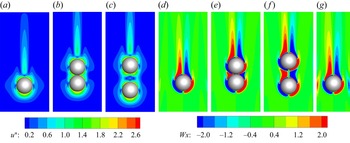
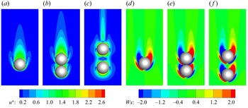
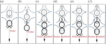
Figures 6 and 7 compare the velocity and vorticity around the squirmers and squirmer dumbbells with β = ±3 at steady speeds of Re = 25. Note that the velocity magnitude of these flow fields is normalized with U 0 = 2B 1/3. A more efficient downstream advection of the vorticity generated on the surfaces of the bodies is observed for the pusher and pusher dumbbell (see figure 6d,e, f), compared with that for the puller and puller dumbbell (see figure 7d,e, f). This is because of the different swimming modes such that the pusher and pusher dumbbell ‘push’ the flow away from their bodies, whereas the puller and puller dumbbell ‘pull’ the flow to accumulate around their bodies. As the squirmers in the front and rear of a dumbbell generate opposite flows in the adjacent area, we can observe that both the velocity magnitude and the vorticity are weakened there. Hence, if we use arrows with magnitudes to represent the flow, the arrows in this area will be smaller, as shown in figure 8.
Comparing the flow fields around the pusher and pusher dumbbells with β = −3 at Re = 25. (a–c) Velocity magnitude contours; (d–g) vorticity contours. (b,e) Denote the pusher dumbbell with ds = 2a; (c, f) denote the pusher dumbbell with ds = 3a; (g) κ = 0.5. The velocity magnitude is normalized with 2B 1/3.

Comparing the flow fields around the puller and puller dumbbells with β = 3 at Re = 25. (a–c) Velocity magnitude contours; (d–f) vorticity contours. (b,e) Denote the puller dumbbell with ds = 2a; (c, f) denote the puller dumbbell with ds = 3a.

Schematic to compare the swimming mechanisms between an individual inertial squirmer and squirmer dumbbells swimming inside a tube. (a) A puller; (b) a pusher; (c) a puller dumbbell with ds = 2a; (d) a pusher dumbbell with ds = 2a; (e) a puller dumbbell with ds = 3a; ( f) a pusher dumbbell with ds = 3a. The dashed and solid squirmers and squirmer dumbbells respectively denote them at the previous and current instants. The dashed and solid boundary lines respectively represent the periodic and no-slip conditions. All the blue arrows indicate the flows induced at the previous instant, and the black arrows denote the flows affecting the squirmers and squirmer dumbbells at the current instant. Due to the hydrodynamic interaction between the adjacent squirmers of the dumbbells, the flows near the joints are weakened and denoted with smaller arrows as shown in (c), (d), (e) and ( f). The flows are more weakened for squirmer dumbbells with ds = 2a than ds = 3a. As both the squirmer and squirmer dumbbell are swimming inside an identical tube, the effect of the tube walls is not taken into account.

To illustrate the effect of inertia on the swimming speeds of the squirmer and squirmer dumbbell, a schematic comparing the swimming mechanism of an individual squirmer and a squirmer dumbbell is shown in figure 8. As an inertial puller is ‘pulled’ by the flows it induced earlier (denoted by the solid arrows as in figure 8a), the inertial puller dumbbell is ‘pulled’ by the flows with a smaller intensity (the sum of the hindering effect by the solid arrows (see figure 8c) is weaker than that shown in figure 8(a), and the mass of the puller dumbbell is greater than an individual puller). Hence, the puller dumbbell can swim faster than an individual puller. As an inertial pusher is ‘pushed’ by the flows it induced earlier (denoted by the solid arrows in figure 8b), the inertial pusher dumbbell is pushed by the flows with a smaller intensity (the sum of the hastening effect by the solid arrows (see figure 8d) is weaker than that shown in figure 8(b), and the mass of the pusher dumbbell is greater than an individual pusher). Hence, the pusher dumbbell swims slower than an individual pusher. Note that, since both the squirmer and squirmer dumbbell are swimming inside identical tubes, we consider the equivalent effect of the tube walls when discussing the effect of the fluid inertia.
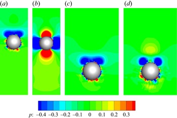
In addition, the pressure fields around the swimmers may also be helpful in understanding their swimming mechanisms, as shown in figure 9. It is seen that a puller (dumbbell) is subject to a negative pressure on its rear, which may tend to pull the body backward. In contrast, a pusher (dumbbell) suffers a nearly fore-and-aft symmetrical positive pressure. This may be the cause of an inertial pusher (dumbbell) swimming faster than the counterpart puller (dumbbell) (see figure 4). Meanwhile, the contacted pullers forming the dumbbell (ds = 2a) occupy the negative pressure induced by the front puller (see figure 9b), resulting in a faster puller dumbbell than an individual puller (each puller of the dumbbell suffers smaller positive pressure than that for the individual puller). Similarly, the contacted pushers forming the dumbbell (ds = 2a) occupy the positive pressure induced by the front pusher (see figure 9e), corresponding to a weakened flow (see figure 8d) between the pushers.
Comparing the pressure fields around the squirmers and squirmer dumbbells at Re = 25. (a–c) Puller and puller dumbbells with β = 3; (d–f) pusher and pusher dumbbells with β = −3.

4.2. Constrained tube can hasten an inertial pusher and pusher dumbbell and a larger ds results in a slower (faster) inertial pusher (puller) dumbbell
For a squirmer swimming inside a tube at Re = 0, an enhanced blocking ratio (κ = a/R) results in a slower speed regardless of β (Zhu et al. Reference Zhu, Lauga and Brandt2013). At finite Re, inertial flow and the tube constraint competitively affect the swimming of the squirmer and squirmer dumbbell, leading to different speeds depending on β, as shown in figure 10. Figure 10a presents the speed of the squirmer as a function of Re with κ = 0.2, 0.33 and 0.5. Note that we define the three κ values as the weak (κ = 0.2), the medium (κ = 0.33) and the strong (κ = 0.5) tube constraints, respectively.
Steady swimming speeds for the swimmers as a function of κ and ds at typical Re. (a) Squirmer; (b) squirmer dumbbell.

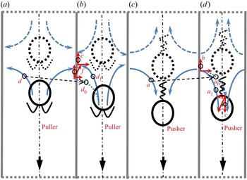
It is seen in figure 10(a) that the speed of the squirmer is hindered within the strong tube constraint, compared with that in the weaker constraints. This is because the tube constraint rather than the fluid inertia dominates the speeds of the squirmers with κ = 0.5. This hindering is more pronounced for the pusher with β = −3 than that for the puller with β = 3, corresponding to a decrease of speeds of more than 50% (pusher) and less than 12% (puller) at Re = 25, respectively. Interestingly, in figure 10(a), the speed of the pusher displays a non-monotonic variation when decreasing κ from 0.33 to 0.2; This is one of the main findings in this section. The physical mechanism for this result can be elaborated in two stages with increasing Re. At finite but low Re (Re ≤ 25, see figure 10a), the effect of the tube constraint (any κ in this study) on the swimming is greater than that of the inertial flow. Hence, the greater the κ, the slower the speed of a pusher, similarly to the swimming in the Stokes flow regime (Zhu et al. Reference Zhu, Lauga and Brandt2013). At higher Re (Re > 25, see figure 10a), the swimming mechanism can be illustrated through the schematic shown in figure 11. As an inertial pusher is ‘pushed’ by the flows it induced earlier (denoted by the solid arrows in figure 11c,d), increasing κ (from the weak tube constraint to the strong tube constraint) leads to an increase of the inertial flow, increasing its speed. The increase inertial flow in the direction of the z-axis is denoted by twice the magnitude of the red arrow c (see figure 11d). Note that we provide a duplicate of the arrow a (see figure 11c) as arrow a 0 (see figure 11d) to better demonstrate the variation of the inertial flow (a 1 denotes half of the inertial flow hastening the speed of a pusher with enhanced κ). Moreover, the increased effect of no-slip tube walls in hindering the speed of the pusher is represented by twice the magnitude of the red arrow b. Therefore, the competitive effects of the inertial flows and the tube constraints are determined by comparing the magnitudes of the red arrows b and c. When increasing κ from the weak constraint to the medium constraint at a specified Re, the inertial pusher swims faster (slower) if the magnitude of arrow c is greater (smaller) than that of arrow b, corresponding to our result that the pusher with β = −3 swims slower (faster) at Re ≤ 25 (Re > 25), as shown in figure 10(a). It can also be implied that, for the pusher, the magnitude of arrow c is smaller than that of arrow b when increasing κ from the medium constraint to the strong constraint.
Schematic to compare the swimming mechanisms for an inertial squirmer swimming inside a tube with different κ. (a,c) A smaller κ; (b,d) a greater κ. The dashed and solid squirmers, respectively, denote them at the previous and current instants. All the blue arrows indicate the flows induced at the previous instant, and the black arrows denote the flows affecting the squirmers at the current instant. The red arrows e and b denote the enhanced hindering of the no-slip walls when increasing κ; The red arrows c and f denote the variation of the inertial flows when increasing κ. This schematic is adaptable to indicate the swimming mechanism of the squirmer dumbbell.

Similarly, an inertial puller is ‘pulled’ by the flows it induced earlier (denoted by the solid arrows as in figure 11a,b), and increasing κ leads to an increase in the inertial flow, hindering its speed. This increase in the direction of the z-axis is denoted by twice the magnitude of the red arrow f (see figure 11b). We provide a duplicate of arrow d (see figure 11a) as d 0 (see figure 11b) to demonstrate the variation of the inertial flow (d 1 denotes half of the inertial flows hindering the speed of a puller with an enhanced κ). As both the arrows e and f are opposite to the swimming direction, it can be concluded that, the greater the κ, the smaller the speed of the inertial puller. These conclusions for the squirmers are also applicable for the counterpart squirmer dumbbells (see figure 10b) because they have the identical swimming mechanism.
Another main finding is that, as shown in figure 10(b), a greater ds results in a slower speed for a pusher dumbbell and a faster speed for a puller dumbbell. It is seen that the vorticity between the two pushers of the dumbbell is inhibited more with ds = 2a than with ds = 3a (see figure 6e, f). Hence, we employ a schematic to indicate the hydrodynamical effect without loss of generality when altering ds, as shown in figure 8. The more inhibited flow denoted by the solid arrows with ds = 2a (see figure 8d) contribute to a greater inertial flow, hastening the pusher dumbbell compared with that with ds = 3a, as shown in figure 8( f). The inertial flow, denoted by the joint action of all the solid arrows, is determined by the solid arrows opposite to the swimming direction as the ones in the swimming direction are considered equivalently. Looking to figure 8(d, f), a greater ds corresponds to greater arrows opposite to the swimming direction because of the weaker constraint. Hence, the pusher dumbbell with smaller ds swims faster.
Similarly, the vorticity between the two pullers of the dumbbell is inhibited more with ds = 2a than with ds = 3a (see figure 7e, f). The more inhibited flow denoted by the solid arrows opposite the swimming direction with ds = 2a (see figure 8c) leads to a more powerful inertial flow, hindering the puller dumbbell compared with with ds = 3a (see figure 8e). Hence, the puller dumbbell with greater ds swims faster.
By increasing κ, as shown in figure 12(a), the variation of the negative pressure at the rear of the puller is not seen to be appreciable (refer to figures 9a and 12a); hence, its speed dose not vary significantly. In contrast, the positive pressure at the rear of the pusher is weakened (refer to figures 9d and 12b), causing a drastic drop in its speed when increasing κ from 0.33 to 0.5 (see figure 10a). Meanwhile, we also plot the vorticity around the pusher. It is seen in figure 6(g) that a distinct vorticity is generated at the narrow tube walls, which may play a significant role in hindering the speed of the pusher.
Comparing the pressure fields around the squirmers. (a) Puller (β = 3) with κ = 0.5 (Re = 25); (b) pusher (β = −3) with κ = 0.5 (Re = 25); (c) puller (β = 3) with κ = 0.33 (Re = 25); (d) puller (β = 3) with κ = 0.33 (Re = 80).

4.3. Velocity decay and analysis of swimming stability
The velocity decay of the flow field in front of the squirmer and the squirmer dumbbell can provide additional insight into understanding the effect of both the fluid inertia and the tube walls on their swimming. For a steady swimming in an infinite fluid field at Re = 0, the flow velocity in front of the squirmer decays as  $|\boldsymbol{u} |\approx O({r^{ - 2}})$, because the two terms on the right-hand side of (2.9) represent a potential dipole which decays as
 $|\boldsymbol{u} |\approx O({r^{ - 3}})$ and a stresslet which decays as |
 $|\boldsymbol{u} |\approx O({r^{ - 2}})$. Accordingly, a swimming squirmer dumbbell at Re = 0 is considered as a couple of potential dipoles and stresslets appropriately arranged in tandem. Recent numerical simulations (Li et al. Reference Li, Ostace and Ardekani2016; More & Ardekani Reference More and Ardekani2020) indicate that the fluid velocity in front of the squirmers decays as
 $|\boldsymbol{u} |\approx O({r^{ - 3}})$ at a finite Re.
Figure 13 presents the velocity decay with r from the centre of the squirmer (for the squirmer dumbbell, it is from the centre of the front squirmer). Note that the velocity |u| and the distance r are, respectively, normalized with the characteristic swimming speed 2B 1/3 and the radius a of a squirmer. For a puller with β = 1 swimming inside a tube with κ = 0.33 at Re = 25 (see figure 13a), the velocity decays as  $|\boldsymbol{u} |\approx O({r^{ - 3}})$, in agreement with the result of an identical puller swimming in an infinite flow field (Li et al. Reference Li, Ostace and Ardekani2016). With increasing Re (increasing the inertial effect), the velocity decay with r becomes faster (from approximate O(r −4) to O(r −8) for the pusher (β = −1) and from approximate O(r −2.5) to O(r −3) for the puller (β = 1)). Combined with the swimming speeds as in figure 4(a), this result is in agreement with the conclusion that a more rapid decay leads to a larger efficiency (Zhu et al. Reference Zhu, Do-Quang, Lauga and Brandt2011). For the cases of the squirmer dumbbells at Re = 25, it is seen in figure 13(b) that the velocity decay with |β| = 1 is identical to that of an individual squirmer. With varying β, κ or ds, the velocity decay also follows the above law that the faster the velocity decay of the flow, the faster their speeds are.
Effect of Re, β, κ and ds on the far-field flow structure. (a) A squirmer at different Re; (b) a squirmer dumbbell with different β, κ and ds. Here, r/a gives the location in front of the squirmer or squirmer dumbbell directing the z-axis (as shown in figure 1, r/a = 1 is the location at the surface and in front of the squirmer or squirmer dumbbell).

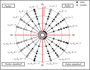
Figure 14 summarizes the stable and unstable motions of a squirmer and a squirmer dumbbell across Re. Recall that the locomotion of the squirmer and squirmer dumbbell vertical to the axial direction of the tube is restricted to obtain a steady swimming speed, and this restriction is removed in this section. At Re = 0, when the squirmer is initially released at the centreline of a tube parallel to the axial direction of the tube, Zhu et al. (Reference Zhu, Lauga and Brandt2013) have found that a puller (β > 0) tends to move away from the nearest wall whereas a pusher (β < 0) tends to move towards the nearest boundary. This finding indicates the different swimming stabilities (in this section, we consider a motion maintaining the original orbit as stable swimming and motion off the original orbit as unstable) for a squirmer with different β, and its physical mechanism has not been fully answered. We illustrate the mechanism through a schematic, as shown in figures 15(a) and 15(b), first. Note that the swimming stability mechanism of the squirmer is also adaptable to the counterpart squirmer dumbbell. A puller is initially swimming along the centreline (see figure 15a for the dashed puller and the induced flow). If a random perturbation leads to departure from the centreline, the flow induced by the puller changes due to the tube wall restriction (see the solid puller and the induced flow). Since the red arrow a has a greater magnitude than the red arrow b (the red arrows denote the components of the flow), the flows tend to pull the puller to return the centreline. For a pusher departing from the centreline by a random perturbation (see figure 15b), the induced flow also changes due to the tube wall restriction (see the solid pusher and the induced flow), leading to pushing of the body closer to the sidewall of the tube (the red arrow d has a greater magnitude than the red arrow c).
A polar phase diagram indicating the stable and unstable squirmers and squirmer dumbbells with different κ and ds; κ 1 = 0.2, κ 2 = 0.33, κ 3 = 0.5; ds 1 = 2a, ds 2 = 3a.

Schematic to reveal and compare the swimming stability between the puller and pusher in a tube. The dashed and solid squirmers, respectively, denote them at the previous and current instants. The solid and dashed blue arrows in (a) and (b) respectively denote the flows induced at the previous and current instants; for the Stokes flow, the previous flows do not affect the swimming of the squirmers at the current instant; The red arrows a–d denote the components of the current flows. The blue arrows in (c) and (d) respectively denote the flows induced at the previous instant, and the black arrows represent the flows affecting the squirmers at the current instant; for the swimming of the inertial squirmers, the extra flow (red arrows f and g) results from the inertial flows at the previous instant. This schematic is adaptable to indicate the swimming mechanism of the squirmer dumbbell.

This swimming stability of a squirmer becomes complex with the inclusion of inertia. In a bulk fluid, an inertial puller (pusher) perturbed from its straight-line trajectory is pushed away (pulled towards) the original trajectory due to the flow induced earlier, making it unstable (stable) with increasing Re (Li et al. Reference Li, Ostace and Ardekani2016; More & Ardekani Reference More and Ardekani2020). Hence, for the inertial squirmer swimming inside a tube, both the inertial flow and the tube constraint competitively affect the swimming stability, as shown in figures 15(c) and 15(d). The red arrows f and g (the two components of the left inertial flow (solid blue arrow) vertical to the tube wall) denote the effect of the inertial flow in a tube. The sum of arrows b and f (c and g) is compared with that of arrow a (d), to find the motion in the next instant (that of the greater one).
Looking back to figure 14, it is seen that the increase of Re tends to make the pullers unstable. This is because the increased inertia of the fluid amplifies the arrow f, leading to a total effect of the flow in pulling the body towards the sidewall (becomes unstable). With increasing β, this unstable motion occurs earlier with Re (see figure 14, the puller with β = 1 at Re = 25 is stable, whereas the one with β = 3 becomes unstable), because the increased β enhances the effect of the fluid inertia. An inertial puller is more stable with a greater κ, as shown in the first quadrant of figure 14, because the effect of the inertial flows becomes weaker compared with the effect of the tube constraint with greater κ. In addition, as shown in figures 12(c) and 12(d), an enhanced Re changes the negative pressure distribution at a puller's rear (the negative pressure is now split), and a positive pressure is generated downstream of the body. This interaction between the positive and negative pressures may be the cause of unstable swimming.
The puller dumbbell is more stable than the counterpart puller – this is because the averaged inertial flow (the flow on the unit mass of a swimmer) induced by the puller dumbbell in pulling the body away from the original orbit is smaller than that induced by the puller (Ouyang & Lin Reference Ouyang and Lin2021). For the pusher and pusher dumbbell swimming in the tube with κ = 0.33, their motions become stable at Re = 5 and then unstable at Re = 10. This may result from the subtle (non-monotonic change) competitiveness between the inertial flow and the tube constraint. Still, when increasing κ, the pusher and pusher dumbbell are seen to become more unstable at the identical Re, indicating that the enhanced tube constraint leads to hindering of the swimming inertia of an inertial swimmer.
In the unstable swimming mode, the swimmers will collide with the wall. In addition to hydrodynamic interactions, we implement a soft-sphere collision model to resolve the short-ranged collisions. It calculates a repulsive force between the ith and jth objects that are close to contact as Lin & Gao (Reference Lin and Gao2019)
 \begin{equation}{\boldsymbol{f}_{ij}} = {\kappa _0}\left( {1 - \frac{d}{{{d_c}}}} \right)\boldsymbol{n},\end{equation}
where the constant κ 0 is typically chosen as 103–104 of the particle mass, d is the particle interdistance, dc is a cutoff distance to define the ‘contact’ zone which is dependent on mesh size Δx (typically dc = Δx~2Δx) and n is a unit vector pointing in the direction where contact occurs. We have tested the squirmer and squirmer dumbbell trajectories, finding that their motion relies on the initial conditions (the orientation and the position). Meanwhile, as a squirmer or squirmer dumbbell has six degrees of freedom in the three-dimensional space, we find an unstable squirmer and squirmer dumbbell display chaotic trajectories beyond a critical Re (between 20 and 30). These results may be because of the intrinsic numerical imprecision of our code when the swimmer and the tube wall are very close (we use the simplified collision model rather than a direct simulation using a mesh with a very high resolution). For this reason, we have to restrict the swimmers to the x-z plane (see figure 1) to obtain periodic trajectories.
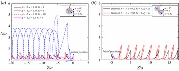
As shown in figure 16, the swimmers periodically oscillate near the wall. This typical trajectory is also observed for a squirmer swimming near a sidewall (Li & Ardekani Reference Li and Ardekani2014). With increasing Re, a swimmer tends to break free of wall attraction. A wider tube (e.g. κ = 0.2) yields swimming closer to the wall, as the effect of the sidewall becomes significant. In addition, a pusher dumbbell with a larger ds yields a larger oscillation amplitude. This may be caused by the dumbbell's large rotation amplitude (with a large ds). Note that the initial position and orientation of the swimmers are indicated in the inset of figure 16.
Typical trajectories for a pusher and pusher dumbbell swimming inside a tube. (a) Pusher; (b) pusher dumbbell. The initial position and orientation of the swimmers are indicated in the inset.

4.4. Swimming power and hydrodynamic efficiency
For a squirmer (squirmer dumbbell) swimming in a viscous liquid, the rate of work P can be written as
 \begin{equation}P ={-} \int_S {(\boldsymbol{u}\boldsymbol{\cdot }\boldsymbol{\sigma })\boldsymbol{\cdot }\boldsymbol{n}\,\textrm{d}S} ,\end{equation}
where n is the unit normal outward from the surface S of the squirmer (squirmer dumbbell), σ is the stress tensor. Similar to the hydrodynamic efficiency introduced by Blake (Reference Blake1971), we define it for the squirmer (squirmer dumbbell) as  $\eta = \boldsymbol{F}\boldsymbol{\cdot }{\boldsymbol{U}_G}\textrm{/}P$, where F is the force on the passive sphere (or the dumbbell) (without the given tangential velocity as (2.10)) from the fluid, when dragged with a corresponding constant velocity UG. Figure 17(a) presents the power expenditure as a function of Re for the squirmer and squirmer dumbbell swimming inside a tube with κ = 0.33; P* denotes P normalized with
 $4B_1^2\mu a\textrm{/}9$. It is apparent from figure 17(a) that P for the inertial squirmer is enhanced with the increase of the swimming intensity |β|, similarly to that of a squirmer swimming in an infinite fluid field at Re = 0 (Wang & Ardekani Reference Wang and Ardekani2012; Chisholm et al. Reference Chisholm, Legendre, Lauga and Khair2016). This is because of the increased vorticity generation by the second term on the right of (2.9). As Re is increased, the increased vorticity around the body also leads to the monotonic increase of P. As expected, the squirmer dumbbell expends more energy than an individual squirmer. It is seen in figure 17(b) that a greater ds or smaller κ results in expenditure of less energy for the squirmer dumbbells. This is because increasing ds or decreasing κ leads to less viscous dissipation. Figure 18 presents the hydrodynamic efficiency η as a function of Re. It is seen that an inertial pusher swimming inside a tube is more efficient than an inertial puller, in agreement with the result when swimming in the bulk fluid (Chisholm et al. Reference Chisholm, Legendre, Lauga and Khair2016). The result that increasing |β| results in a lower swimming efficiency (Chisholm et al. Reference Chisholm, Legendre, Lauga and Khair2016) has also been reproduced. For the inertial squirmer dumbbell, a higher η is observed with a greater ds, because more power is expended ineffectively due to the hydrodynamic interaction between the squirmers of the dumbbell when they are arranged closer to each other (Ouyang & Lin Reference Ouyang and Lin2021). Moreover, we observe that η of the pusher dumbbell becomes higher with the increase of κ, as shown in figure 18(b).
Power expenditure for swimming inside the tubes as a function of Re. (a) Squirmers and squirmer dumbbells in a tube with κ = 0.33; (b) squirmer dumbbells with different ds in different tubes.

Hydrodynamic efficiency for swimming inside the tubes as a function of Re. (a) Squirmers and squirmer dumbbells in a tube with κ = 0.33; (b) squirmer dumbbells with different ds in different tubes.

5. Conclusion
A direct numerical simulation study on the hydrodynamics of a spherical and dumbbell-shaped inertial swimmer in a tube is conducted in this paper. We use the reduced squirmer model with a tangential velocity on the boundaries to mimic the locomotion mechanism of the swimmer. The dumbbell-shaped swimmer is assembled by two squirmers appropriately in tandem. The main innovation of this work is to reveal how the fluid inertia and the tube constraint competitively affect the hydrodynamics of these two types of swimmers. We hence consider the swimming speed, the velocity decay of flow field, the swimming stability, the power expenditure and the hydrodynamic efficiency of inertial swimmers with different swimming Reynolds numbers (Re), blockage ratios (κ) and relative distances (ds) of the squirmer dumbbells.
It is found that, inside a tube, the squirmer dumbbell weakens the effect of the fluid inertia more than an individual squirmer. Hence, the inertial pusher dumbbell swims slower than the individual pusher, whereas the inertial puller dumbbell swims faster than the individual puller. This is because the inertial pusher dumbbell suffers smaller inertial flow per unit mass to speed up the body than an individual pusher, whereas the inertial puller dumbbell suffers greater inertial flow per unit mass to hinder the body than an individual puller.
We find a medium constrained (κ = 0.33) tube can speed up an inertial pusher and pusher dumbbell at Re ≥ 50. This is because the joint effects of the fluid inertia and the tube constraint (e.g. at κ = 0.33 when Re ≥ 50) in speeding up the body are more pronounced than that for the weak (κ = 0.2) and strong (κ = 0.5) tube constraints. It is seen that a greater ds results in a slower (faster) speed of an inertial pusher (puller) dumbbell. This is because a pusher dumbbell with greater ds contributes to a smaller ‘pushing’ (‘pulling’) effect to hasten (hinder) the body due to the hydrodynamic interaction between the adjacent pushers.
Subsequently, we comprehensively illustrate why a puller (β > 0) inside a tube tends to move away from the nearest wall, whereas a pusher (β < 0) tends to move toward the nearest boundary. With increasing Re, we find that both the fluid inertia and the tube constraint competitively affect the swimming instability of the squirmer and squirmer dumbbell. The increase in Re tends to make the puller and the puller dumbbell unstable due to the enhanced inertial effect, and an inertial puller and puller dumbbell are more stable with a greater κ due to the weakened inertial flow.
In addition, we present and discuss the swimming power and hydrodynamic efficiency for the squirmer and squirmer dumbbell swimming inside a tube. We find the swimming power and hydrodynamic efficiency of the swimmers depend on the blockage ratios (κ), and the relative distances (ds). A greater ds or smaller κ results in less energy expenditure for the squirmer dumbbell, and η of the pusher dumbbell becomes higher with the increase of κ.
Acknowledgements
The authors would like to thank the Major Program of National Natural Science Foundation of China (Grant No. 12132015), the Fundamental Research Funds for the Central Universities of China (Grant No. 2020QNA4046) and National Natural Science Foundation of China (Grant No. 12072319).
Declaration of interests
The authors report no conflict of interest.
Data availability statement
The data that support the findings of this study are available from the corresponding author upon reasonable request.