


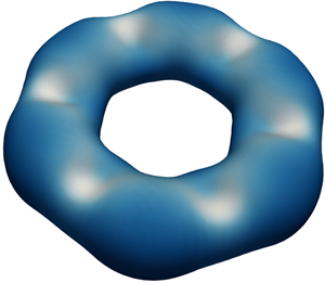



1. Introduction
Vortex rings appear in a variety of flows when the vorticity in a layer adjacent to a surface separates and rolls up, like at the exit orifice of a nozzle. In living systems, for example, such rings appear at the periphery of a fluid parcel ejected from the mouth of a system. In round jets the separating sheet of vorticity is inviscidly unstable to small perturbations, and the ensuing redistribution results in vorticity accumulating into rings while also being depleted between successive rings. The initial inviscid instability is a form of the linear Kelvin–Helmholtz instability of vortex sheets, while the subsequent roll-ups into rings is essentially a nonlinear process. Vortex rings are themselves unstable to azimuthal perturbations, whose inviscid asymptotic theories were developed in Widnall & Sullivan (Reference Widnall and Sullivan1973) and Widnall, Bliss & Tsai (Reference Widnall, Bliss and Tsai1974), for slender rings whose core radius  $a \ll R$, the ring radius. These were later extended to viscous flows (Eloy & Le Dizés Reference Eloy and Le Dizés2001; Fukumoto & Hattori Reference Fukumoto and Hattori2005), while viscous growth rates have also been extracted from direct numerical simulations (DNS) (Shariff, Verzicco & Orlandi Reference Shariff, Verzicco and Orlandi1994; Archer, Thomas & Coleman Reference Archer, Thomas and Coleman2008; Hattori, Blanco-Rodríguez & Le Dizés Reference Hattori, Blanco-Rodríguez and Le Dizés2019). In this work a detailed global, modal stability analysis of vortex rings for both inviscid and viscous flows is performed where one of the primary aims is to clarify some of the existing discrepancies between asymptotic theories and numerical simulations.
In a series of works with asymptotic theories of inviscid vortex rings, Widnall & Sullivan (Reference Widnall and Sullivan1973) first considered  $\epsilon = a/R \ll 1$ and uniform vorticity across the ring core to show such vortex rings to be neutrally stable as
 $a \rightarrow 0$. Here, the lowest ring azimuthal modes
 $n=0,1$ have zero growth rates, while the higher modes were shown to execute periodic oscillations. Results of Widnall & Sullivan (Reference Widnall and Sullivan1973) agreed with earlier results of Kelvin (see Thomson Reference Thomson1880, Reference Thomson1883), while further demonstrating a particular
 $n$ to be unstable over non-overlapping ranges of small, but finite, slenderness ratios
 $\epsilon$. These values of
 $n (\ge 2)$ increased monotonically with a decrease in
 $\epsilon$. Although the theoretical growth rates matched well with the findings from initial experiments, the azimuthal mode numbers
 $n$ deviated. Moreover, the predicted instabilities were essentially for short waves that clearly violated the requirement of small variations along the ring compared to across its core. Later, when Widnall et al. (Reference Widnall, Bliss and Tsai1974) accounted for short waves, predictions for
 $n$ improved. It was argued that instabilities occur when the self-induced rotation rate of the vortex filaments vanishes, a condition apparently met only for the higher radial modes. This yielded better agreements with the experiments once the instability was estimated from the second radial mode.
An important contribution was due to Widnall & Tsai (Reference Widnall and Tsai1977), who considered the systematic development of asymptotic theory for the inviscid vortex ring instabilities with small  $\epsilon$ as the order parameter. They obtained the essential mechanism of vortex ring instabilities at
 $O(\epsilon ^2)$ due to a resonance between mode pairs, to be similar to a line vortex in the strain field due to a second vortex (Moore & Saffman Reference Moore and Saffman1975; Tsai & Widnall Reference Tsai and Widnall1976). This instability occurs for azimuthal mode pairs of the same frequency and axial wavenumbers which is satisfied at intersections of dispersion curves for fixed azimuthal modes. Expectedly, the maximum growths occur here at the zero frequencies. These belong to a class of instabilities termed as elliptical instability, found in flows with elliptic streamlines (Kerswell Reference Kerswell2002). Note that although the ring curvature is an
 $O(\epsilon )$ effect, there is still no destabilization, while the corresponding correction is just proportional to the lowest-order stable solution. The calculated growth rates therefore include a small contribution from the curvature effect. However, Fukumoto & Hattori (Reference Fukumoto and Hattori2005) have argued that curvature effects can still destabilize a ring in an inviscid flow for a mode pair in resonance when the azimuthal modes differ by 1, with an
 $O(\epsilon )$ velocity field. Although, unlike the instability due to strain, the most unstable mode of curvature instability occurs at the short-wavelength limit.
A set of recent advancements on instabilities of vortex rings is due to Blanco-Rodríguez et al. (Reference Blanco-Rodríguez, Le Dizés, Selçuk, Delbende and Rossi2015) and Blanco-Rodríguez & Le Dizés (Reference Blanco-Rodríguez and Le Dizés2016, Reference Blanco-Rodríguez and Le Dizés2017) who extended the asymptotic theories of Widnall & Tsai (Reference Widnall and Tsai1977) and Fukumoto & Hattori (Reference Fukumoto and Hattori2005) for swirling vortex rings with Gaussian distribution. Here, the base velocity fields were computed up to  $O(\epsilon ^2)$, because the non-local effect due to self-induced velocities appear only at
 $O(\epsilon ^2)$ (Blanco-Rodríguez et al. Reference Blanco-Rodríguez, Le Dizés, Selçuk, Delbende and Rossi2015).
Asymptotic theory extensions for viscous instabilities were first included in Eloy & Le Dizés (Reference Eloy and Le Dizés2001), while exploring the response of a vortex in multipolar strain fields as viscosity  $\nu \sim \tau$, where
 $\tau$ is the strength of the strain field. For vortex rings and line vortex pairs, this background strain field is dipolar, while for more general turbulent flows that include influence from neighbouring vortices, a tripolar or quadrupolar model may be used. For a dipolar field, it was found that, for small viscosities, resonance between bending mode pairs (
 $m = \pm 1$, where
 $m$ is the azimuthal mode of the line vortex) is selected, while the pair of bulging (
 $m = 0$) and splitting modes (
 $m = 2$) dominate at larger viscosities, before being cut-off at a critical viscosity. Fukumoto & Hattori (Reference Fukumoto and Hattori2005) showed that when viscosity is included, curvature effects become effective above a critical Reynolds number, larger than the critical
 $Re$ of instability due to strain, which again increases with a decrease in the slenderness ratio
 $\epsilon$. Viscous effects and the effect of curvature on the growth rates of elliptic instabilities were also considered in Blanco-Rodríguez & Le Dizés (Reference Blanco-Rodríguez and Le Dizés2016, Reference Blanco-Rodríguez and Le Dizés2017).
Direct numerical simulations of vortex rings were performed by Shariff et al. (Reference Shariff, Verzicco and Orlandi1994) who extracted growth rates during the early stages of unstable evolution. The initial condition was that of a Gaussian vorticity distribution over the core with small amplitude azimuthal perturbations superimposed. However, in two of the 18 cases reported by Shariff et al. (Reference Shariff, Verzicco and Orlandi1994), perturbations were added to an equilibrated ring that was obtained by allowing the Gaussian distribution to evolve to a nearly steady state. There were qualitative agreements with the inviscid results of Widnall & Tsai (Reference Widnall and Tsai1977), but the corresponding growth rates were less, which was attributed to viscosity. Subsequently, Archer et al. (Reference Archer, Thomas and Coleman2008) also performed DNS of vortex ring evolution, including two cases with the same initial conditions as Shariff et al. (Reference Shariff, Verzicco and Orlandi1994), but found still smaller growth rates which they attributed to the use of axially periodic boundary conditions by Shariff et al. (Reference Shariff, Verzicco and Orlandi1994). The shed vorticity of the initial ring was superimposed on the adjacent rings which seem to have altered the instability growth rates. Gargan, Rudman & Ryan (Reference Gargan-Shingles, Rudman and Ryan2016) integrated the linearised Navier–Stokes equations beginning with an equilibrated velocity field due to a vortex ring, and extracted growth rates which were in between the DNS of Shariff et al. (Reference Shariff, Verzicco and Orlandi1994) and Archer et al. (Reference Archer, Thomas and Coleman2008). Recently, Hattori et al. (Reference Hattori, Blanco-Rodríguez and Le Dizés2019) considered linearised and full Navier–Stokes equations to study the evolution of base flow and perturbations for swirling vortex rings, where curvature instability was found to dominate at large and small values of  $Re$ and
 $\epsilon$, respectively. Even though curvature instabilities are not explored in our work, a few of our unstable modes are similar to the spiral modes of Hattori et al. (Reference Hattori, Blanco-Rodríguez and Le Dizés2019), as we show in § 3.3.
In this work we perform global, linear stability analyses of vortex rings, both at finite  $Re$ and inviscid conditions, for a range of slenderness ratios
 $\epsilon$. To be consistent with the asymptotic analyses of Widnall & Tsai (Reference Widnall and Tsai1977) and Blanco-Rodríguez & Le Dizés (Reference Blanco-Rodríguez and Le Dizés2016), we use a base flow obtained after solving the Poisson equation and further evolving it to yield a skewed Gaussian vorticity distribution, which we refer to as the equilibrated vortex ring. In addition, the Gaussian distribution by itself is also used as a second base flow. Such a global stability analysis may have been difficult earlier because of the large eigenvalue problems that must be solved for correct solutions. Initially, we use these solutions to assess the quantitative accuracies of previous asymptotic solutions for the inviscid instability of slender rings. Since typical unstable vortex rings in round jets are neither quite slender, nor are inviscid, we also extend our calculations to viscous and thicker rings. For some cases, we have done DNS to assess the accuracies of our stability solutions.
The results of present modal analysis are entirely consistent with the theories of Widnall & Tsai (Reference Widnall and Tsai1977) and Blanco-Rodríguez & Le Dizés (Reference Blanco-Rodríguez and Le Dizés2016), and show the same qualitative trends in both inviscid and viscous analyses. Our calculations with equilibrated vortex rings show that small differences in the vorticity distribution, due to equilibration carried out at different Re, of these rings can give a  $\sim$9 % difference in growth rate for
 $\epsilon \approx 0.29$ and
 $\sim$3.5 % for
 $\epsilon \approx 0.19$. However, in spite of these differences, the growth rates from inviscid modal analysis with equilibrated vortex rings are found to be quite close to the asymptotic theories of Widnall & Tsai (Reference Widnall and Tsai1977) and Blanco-Rodríguez & Le Dizés (Reference Blanco-Rodríguez and Le Dizés2016) (range of differences being
 $\sim$0.1–10 % and
 $\sim$2–5 % for thicker and thinner rings, respectively, also depending upon which asymptotic theory we compared against). There are, however, several quantitative differences between the asymptotic theory and the results of inviscid modal analysis for inviscid instability of Gaussian rings. Generally, growth rates from inviscid modal analysis are
 $\sim$14–33 % smaller than that from the asymptotic theories over a range of
 $\epsilon \sim 0.4$–0.05. In this work we explore in detail the origin of these differences which will be primarily attributed to the respective nature of the vorticity and induced velocity distributions.
In what follows, the base flows for the stability equation are discussed and analysed in § 2. The equilibrated base flow follows from the incompressible flow DNS and these are described in §§ 2.1 and 2.2, while the Gaussian base flow is in § 2.3. The base flows are analysed and compared in §§ 2.4 and 2.5. The global stability results are presented in § 3 with a brief overview of numerical methods in § 3.1. In § 3.2 we assess the accuracy of our global stability results by comparing with our DNS results, while § 3.3 contains a summary of all the important results of this work, which are directly compared with other relevant data from the literature where a new viscous correction is also introduced. Growth rates are seen to be smaller and occurring for a smaller range of modes as  $Re$ is decreased, with the instabilities disappearing below a critical
 $Re$. The fact that our calculated inviscid growth rates are different from the asymptotic theories for the Gaussian rings is explored in §§ 3.4 and 3.5, where the effects of base flow vorticity distribution and slenderness ratios, respectively, on inviscid growth rates are demonstrated. Here, equilibrated vortex rings are shown to yield growth rates that are very close to theoretical predictions. The effects of viscosity are further discussed in § 3.6 while the conclusions are in § 4. Finally, appendix A describes the standard stability equations, corresponding eigenvalue problem and details of the stability matrices, while appendix B shows the validation and convergence studies of our global stability solver and appendix C discusses the stability of line vortices and their dispersion curves showing the connection with stability of vortex rings.
2. Stability problem base flows
In this work we use a Cartesian box  $(x,y,z)$ within which the undisturbed ring is placed, as used in the DNS, but also in our stability calculations where a Poisson solver initially yields the base flow velocity distribution (see figure 1a,b). In our simulations the ring travels along the ring axis (i.e.
 $x$-axis), while its positions on the transverse
 $y$–
 $z$ plane are also described via its polar coordinates
 $(r,\theta )$. The latter system is primarily used for our stability calculations, as described in the following and visualized in figure 1(a,b). Additionally, the initial azimuthal vorticity distribution over the ring is specified via a second polar coordinate system
 $(s,\phi )$ with its origin at the centre of the ring core (at
 $r = 1, x = x_c$, see figure 1(a), with
 $x_c = 2.5$ fixed for all our stability calculations) and radial ordinate as
 $s = (x^2 + (y-1)^2)^{1/2}$ (see figure 1a). Later, when modal analysis of a line vortex is described in appendix C to connect certain mechanistic similarities between the ring and line vortices, we also use this
 $(s,\phi ,z)$ system, with the line vortex axis located along the
 $z$ direction. Here, quantities are scaled with the initial vortex ring radius
 $R$ of the circle through its core centre and the corresponding circulation
 $\varGamma$. The vortex ring evolution is further specified by a Reynolds number
 $Re = \varGamma /\nu$, where
 $\nu$ is the kinematic viscosity.
The base flow of a typical Gaussian vortex ring as used in this work for  $\epsilon =0.4131$ showing (a) streamlines on the
 $x$–
 $y$ plane in a reference frame moving at the velocity
 ${\rm \Delta} \bar u_x$, (b) the corresponding schematic in the
 $y$–
 $z$ plane, (c) the Gaussian vorticity (
 $\bar \omega _{\theta }$) distribution and (d) the base flow velocity profiles along
 $x = x_c$ (indicated via a vertical dotted line in a) with
 $\bar u_x$ (——) and
 $\bar u_r$ (– – –) indicated. In (a,b) the vortex core is indicated by a grey disk and semi-annulus, respectively (not to scale).

The (Cartesian) solution domain size is  $0 < x < L_x$ and
 $-L_y/2 < y, z < L_y/2$, discretised via
 $N_x \times N_y \times N_z$ equispaced mesh points with
 $N_y = N_z$. The solution is periodic in
 $y$ and
 $z$ while along
 $x$ we use inflow–outflow boundary conditions. The initial velocity distribution is obtained by solving a Poisson problem for the vector potential with each component of vorticity as source terms. In this work this is done using Incompact3d (Laizet & Lamballais Reference Laizet and Lamballais2009; Laizet & Li Reference Laizet and Li2011), a freely available incompressible, viscous flow solver.
2.1. Direct numerical simulations methodology
The base flow for the equilibrated vortex rings (see § 2.2) are obtained from DNS using Incompact3d with Gaussian vorticity core initial conditions. For a Gaussian distribution, the base flow azimuthal vorticity (see figure 1c) is
 \begin{equation} \bar \omega_{\theta}(s) = \frac{1}{{\rm \pi} \epsilon^2} \exp{(-s^2/\epsilon^2)}, \end{equation}
where  $\epsilon = a/R$ is the slenderness ratio, a key parameter for the vortex rings considered here, with
 $a$ being the radius of the vortex core. The DNS for the vortex ring is carried out on the region
 $L_x \times L_y \times L_z = 15 \times 10 \times 10$ via ensuring errors near the outflow region do not affect the flow field in the neighbourhood of the ring. During the simulation, following Archer et al. (Reference Archer, Thomas and Coleman2008), a time varying inflow condition is enforced to maintain the ring stationary with respect to its centroid of enstrophy. Here, two distinct simulations are performed, one for obtaining the equilibrated base flow (discussed next in § 2.2), while the other for extracting the DNS growth rates. For the latter, the initial vortex ring is perturbed along the core centreline via a sum of the first
 $24$ Fourier components, each with unit amplitude and a random phase. For relatively thicker rings, for example, vorticity is shed from the initial ring, following nearly stationary flow before perturbations acquire significant amplitude. Growth rates are then extracted using the procedure detailed in § 3.2 during this nearly stationary flow. Note that our streamwise direction is not periodic so that there is no contamination from adjacent rings of a periodic solution.
2.2. Equilibrated vortex rings
The primary base flow for our stability calculations is also obtained via the technique described in § 2.1, where the initial velocity distribution corresponding to the Gaussian vorticity (2.1) is now evolved for a finite time in the incompressible Navier–Stokes solver without imposing any centreline perturbations. The ring eventually attains a quasi-steady state, after an initial vorticity shedding, and the velocity field at this state is extracted from the region  $x \ge 5$, to ensure consistent geometric properties across all cases considered here, which is then transformed and interpolated using cubic splines to a cylindrical domain
 $L_x \times L_r = 10 \times 5$ (centred on the ring) and averaged azimuthally. This technique yields an equilibrated velocity field (a quasi-steady solution of Euler equations) on the cylindrical
 $(r,\theta ,x)$ grid (see figure 1b) for our stability calculations. This grid is clustered about the vortex ring core using a mapping strategy by Bayliss & Turkel (Reference Bayliss and Turkel1992) and Bayliss, Class & Matkowsky (Reference Bayliss, Class and Matkowsky1995). In this work cases utilizing this particular type of base flow are indicated by the notation
 $E_I()$ or
 $E_V()$, depending on whether the inviscid or viscous stability equations, respectively, are used. For the equilibrated ring, the ring and core radii are obtained from the integrals (Saffman Reference Saffman1970)
 \begin{gather} R_{\theta} = \frac{1}{\varGamma} \int{r \bar\omega_{\theta} \, {\rm d}r \, {\rm d}x}, \end{gather}
 \begin{gather}a_{\theta}^2 = 2(R_2^2 - R_{\theta}^2), \end{gather}
respectively, where
 \begin{equation} R_2^2 = \frac{1}{\varGamma} \int{r^2 \bar\omega_{\theta} \, {\rm d}r \, {\rm d}x},\quad \varGamma = \int{\bar\omega_{\theta} \, {\rm d}r \, {\rm d}x}\quad\textrm{and}\quad r^2 = y^2 + z^2. \end{equation}
For these rings, the slenderness parameter is  $\epsilon ^\ast = a_{\theta }/R_{\theta }$, where such equilibrated quantities for the equilibrated base flow calculations are distinguished with an
 $()^\ast$. In this work, results of stability analysis of the equilibrated ring are compared with the asymptotic results of Widnall & Tsai (Reference Widnall and Tsai1977) and Blanco-Rodríguez & Le Dizés (Reference Blanco-Rodríguez and Le Dizés2016), which would show the growth rates for equilibrated rings to be quite close to that from the asymptotic theories.
2.3. Gaussian vortex rings
A second type of base flow is obtained by adding a uniform axial velocity (Saffman Reference Saffman1970)
 \begin{equation} {\rm \Delta} \bar u_x = \frac{1}{4 {\rm \pi}}\left[\ln \frac{8}{\epsilon} - 0.558\right] \end{equation}
to the velocity distribution corresponding to (2.1), which we also use in this work and denote such cases as  $G_I()$ or
 $G_V()$. Streamlines of a typical Gaussian base flow are shown in figure 1(a). Axial and radial velocity profiles on lines through the centre of the ring's core are shown in figure 1(d). It proved convenient to use this base flow to understand grid requirements and for mode convergence studies that are discussed later in appendix B.2. Gaussian vortex ring results are also used here to compare with previous DNS results of Shariff et al. (Reference Shariff, Verzicco and Orlandi1994) and Archer et al. (Reference Archer, Thomas and Coleman2008) that use a Gaussian vorticity core as the initial condition. A more detailed study of the instability of Gaussian vortex rings are found in Naveen (Reference Naveen2021).
2.4. Comparison of base flows
Recall that the asymptotic theory of Widnall & Tsai (Reference Widnall and Tsai1977) yielded an inviscid steady base flow for the vortex ring for a uniform circular core of azimuthal vorticity along with corrections to  $O(\epsilon )$ and
 $O(\epsilon ^2)$, where the latter correction accounts for the strain rate field that supports the elliptical instability. Later, Blanco-Rodríguez et al. (Reference Blanco-Rodríguez, Le Dizés, Selçuk, Delbende and Rossi2015) obtained the corresponding base flow for a Gaussian core to the leading order. When the velocity field due to a vortex ring with a Gaussian core is obtained by solving the Poisson problem, as described in § 2.3, an
 $O(\epsilon ^2)$ contribution due to non-local effects gets included. A further contribution to
 $O(\epsilon ^2)$ is required due to the
 $O(\epsilon ^2)$ part of the vorticity distribution, which, however, is absent for this base flow. This local
 $O(\epsilon ^2)$ part of the vorticity comes from the deformation of the vortex ring core, which is due to the strain field of induced velocity. Although it naturally appears in the perturbation solutions of Widnall & Tsai (Reference Widnall and Tsai1977) and Blanco-Rodríguez et al. (Reference Blanco-Rodríguez, Le Dizés, Selçuk, Delbende and Rossi2015), being exact solutions of the Euler equation at all orders, the fact that the vorticity distribution (2.1) has only the leading order part precludes its inclusion in the calculated Poisson solutions. A fully consistent base flow is still obtained when the Gaussian vortex is allowed to equilibrate, as described in § 2.2.
For further proof, we now compare the velocity profile from the asymptotic analysis of Blanco-Rodríguez et al. (Reference Blanco-Rodríguez, Le Dizés, Selçuk, Delbende and Rossi2015) with those obtained via solving the Poisson equations. Figures 2 and 3 show this comparison for the equilibrated and Gaussian rings, respectively, up to  $O(\epsilon ^2)$. This is obtained by polar transforming the individual velocity components to
 $(s,\phi )$ (see figure 1a) with its origin at the core centre (i.e. stagnation point), followed by azimuthal Fourier transforms on concentric circles with their centres coinciding with the core centre (more details are in Blanco-Rodríguez et al. (Reference Blanco-Rodríguez, Le Dizés, Selçuk, Delbende and Rossi2015)). In this coordinate system if the radial and azimuthal velocity components are
 \begin{equation} \bar u_s(s,\phi) = \bar u_s^{(0)}(s) + \epsilon \bar u_s^{(1)}(s,\phi) + \epsilon^2 \bar u_s^{(2)}(s,\phi) + \cdots \end{equation}
and
 \begin{equation} \bar u_\phi(s,\phi) = \bar u_\phi^{(0)}(s) + \epsilon \bar u_\phi^{(1)}(s,\phi) + \epsilon^2 \bar u_\phi^{(2)}(s,\phi) + \cdots, \end{equation}
respectively, the assumption of dipole and quadrupole fields at  $O(\epsilon )$ and
 $O(\epsilon ^2)$ yield
 \begin{equation} \bar u_s^{(1)}(s,\phi) = \check{u}_s^{(1)}(s) \sin{\phi},\quad \bar u_\phi^{(1)}(s,\phi) = \check{u}_\phi^{(1)}(s) \cos{\phi} \end{equation}
and
 \begin{equation} \bar u_s^{(2)}(s,\phi) = \check{u}_s^{(2)}(s) \sin{2\phi},\quad \bar u_\phi^{(2)}(s,\phi) = \check{u}_\phi^{(2)}(s) \cos{2\phi}, \end{equation}
respectively, where lengths and velocities are scaled with  $a$ and
 $\varGamma /(2 {\rm \pi}a)$, respectively.
Comparison of velocity fields obtained from the asymptotic analysis of Blanco-Rodríguez et al. (Reference Blanco-Rodríguez, Le Dizés, Selçuk, Delbende and Rossi2015) with the equilibrated ring at (a) leading order, (b)  $O(\epsilon )$ and (c)
 $O(\epsilon ^2)$ for
 $\epsilon ^\ast = 0.1866$. The radial and azimuthal velocity components are shown in thin and thick lines, respectively, with
 , case
 ${E_I5}$ from table 3 and
 $\mbox {- - - -}$, asymptotic analysis (Blanco-Rodríguez et al. Reference Blanco-Rodríguez, Le Dizés, Selçuk, Delbende and Rossi2015). The grey shaded region indicates the vortex core.

 , the


From figure 2, it is clear that the equilibrated ring base flow matches quite well with the asymptotic base flow of Blanco-Rodríguez et al. (Reference Blanco-Rodríguez, Le Dizés, Selçuk, Delbende and Rossi2015), at all  $\epsilon$ orders, especially inside the vortex core. On the other hand, as expected, figure 3 shows that the Gaussian ring base flow profile shows large differences, more so inside the core, except at the leading order, where there is an exact match.
As the elliptic instability occurs due to the velocity field at  $O(\epsilon ^2)$, the difference between the asymptotic and Gaussian base flows at this order is plotted in figure 4 for different
 $\epsilon$ using the relation
 \begin{equation} ()|_d = \sqrt{\{()|_t - ()|_g\}^2}, \end{equation}
where  $()|_t$ and
 $()|_g$ denote base velocity fields from asymptotic analysis and Gaussian rings, respectively. Clearly, the difference at
 $O(\epsilon ^2)$ reduces as
 $\epsilon \rightarrow 0$ (see figure 4), although the form of the velocity profile for the Gaussian rings remains unchanged owing to the absence of core deformation for all
 $\epsilon$.
Difference between the velocity fields obtained from the asymptotic analysis and Gaussian rings at  $O(\epsilon ^2)$ for (a) radial and (b) azimuthal velocity components for different values of
 $\epsilon$:
 (thin),
 $0.4033$;
 $\mbox {- - - -}$ (thin),
 $0.2368$;
 (thick),
 $0.1545$ and
 $\mbox {- - - -}$ (thick),
 $0.0504$. All these cases are tabulated in table 6. The grey region shows the vortex core, while the arrow indicates the direction of increase of
 $\epsilon$.

2.5. Comparison with vortex dipoles
In this context, it is worthwhile to mention the work of Sipp, Jacquin & Cosssu (Reference Sipp, Jacquin and Cosssu2000) which has shown the existence of a family of quasi-steady Euler solutions for the growth of vortex dipoles. They obtained a family of vortex dipoles characterized solely via  $a/b$ (core radius
 $a$, separation
 $b$), irrespective of their initial vorticity distributions (including Gaussian). This follows from the fact that with time, there is very little change in either
 $b$ or
 $\varGamma$, while
 $a$ follows the simple viscous diffusion law
 $a^2 = a_0^2 + 4\nu t$ (
 $a_0$ is the initial core radius). Similar evolution of peak vorticity is also observed, which follows via viscous effects. Unlike in vortex dipoles, the initial slenderness ratio
 $\epsilon$ of the vortex rings is a deciding factor on the nature of their subsequent evolution, which is via two distinct stages.
(a) Vortex shedding. Unlike thinner rings, for thicker vortex rings, the initial period of evolution is dominated by vigorous vorticity shedding leading to a skewed Gaussian distribution (from an initial Gaussian vorticity distribution), which is also sensitive to
 $Re$. This stage is completely absent in vortex dipoles.
(b) Viscous diffusion. Even the effect of viscous diffusion is different for thin and thick rings. For thicker rings,
$\epsilon$ is almost unchanged, as both $a$ and $R$ change at similar rates. For the thinner ring evolution, $a$ directly follows viscous diffusion law, while $R$ remains almost unchanged, thus, very similar to vortex dipole evolution.


It is thus clear that the slenderness ratio of the vortex ring  $\epsilon$ has an important role to play in its evolution (also reported by Archer et al. Reference Archer, Thomas and Coleman2008) and a family of Euler solutions (like vortex dipoles) parametrized via
 $\epsilon$ is not possible here. This may be further confirmed from table 3 in § 3.3 where the thicker ring cases,
 ${E_{I}2}$–
 ${E_{I}4}$, after undergoing equilibration at different initial conditions lead to different solutions at the same
 $\epsilon ^*$, which is even true for the thinner cases (
 ${E_{I}5}$–
 ${E_{I}7}$), although the differences are smaller in the latter (see also figure 10 in § 3.4). Of course, if
 $\epsilon \ll 1$ it is possible to obtain a family of quasi-steady Euler solutions, but our present work is not restricted to this limit.
3. Global stability results
The incompressible global stability equations and the corresponding eigenvalue problem along with the stability matrices are described in appendix A. With the validation and convergence studies of our stability solver deferred to appendix B, some of the important numerical details are first briefly described in § 3.1, before moving to the detailed results and discussion.
3.1. Numerical methods and solutions
Both our base flow Poisson equation solutions and DNS use Incompact3d, which implements high-resolution, sixth-order compact differences for derivatives and third-order Runge–Kutta for time stepping to solve the incompressible Navier–Stokes equations. The solver is known to scale well for up to  ${O}(10^5)$ processors (Laizet & Li Reference Laizet and Li2011). The primary purpose of the DNS is to compare some of the growth rates extracted from these studies with the modal growth rates from our stability calculations, as means of validating the latter (see § 3.2). We also compare our results with the earlier DNS of Shariff et al. (Reference Shariff, Verzicco and Orlandi1994) and Archer et al. (Reference Archer, Thomas and Coleman2008), both of whom had used second-order finite differences in their simulations.
The matrices of the stability equations (A 2) and (A 4) (see (A 5), (A 6), (A8), (A9) and (A11) in appendix A) are discretised using Chebyshev polynomials at their respective Gauss–Lobatto points. In our parallel computations, sub-matrices of (A 5), (A 6) and (A11) are first obtained via the PETSc libraries (see Balay et al. Reference Balay, Gropp, McInnes, Smith, Arge, Bruaset and Langtangen1997; Balay Reference Balay2015a,Reference Balayb) which are then solved using the SLEPc libraries (see Hernandez, Roman & Vidal Reference Hernandez, Roman and Vidal2005; Roman et al. Reference Roman, Campos, Romero and Tomas2017) and MATLAB, which uses the Krylov–Schur iterative algorithm with shift-invert spectral transformation to overcome the singular nature of the matrix (A11).
Boundary conditions on  $\hat {\boldsymbol {q}}$ are specified at the
 $r = 0$ plane as compatibility conditions (Batchelor & Gill Reference Batchelor and Gill1962; Khorrami, Malik & Ash Reference Khorrami, Malik and Ash1989) at the
 $r= L_r$ and
 $x = 0$ surfaces to be
 $\hat {\boldsymbol {q}} = 0$, while values at
 $x = L_x$ are obtained via linearly extrapolating from the two neighbouring interior points.
The stability solver is checked first via reproducing the stability spectrum for the classical Hagen–Poiseuille flow (see appendix B.1). Next, convergence of modes and growth rates are examined with respect to the Gaussian core rings, using cases from table 4 in § 3.3. In each case of our vortex ring stability calculations, as discussed in this section, converged eigenvalues are identified for a specified tolerance with spurious ones discarded first by varying the number of points along the radial and axial directions and then using different shift values during the iterative procedure (full details appear in appendix B.2). The results presented in this work are from discretisations with at least 100 points along both  $x$ and
 $r$ directions. Our inviscid calculations are converged up to a numerical tolerance of at least
 $10^{-2}$, with the thinner rings showing better convergence (
 ${\sim }10^{-4}$), while the viscous calculations are converged up to at least
 $10^{-4}$.
A typical eigenspectrum from these calculations are shown in figure 5 for a Gaussian core vortex ring of  $\epsilon = 0.4131$ (see case
 ${G_{V}1}$ of table 4 in § 3.3) with
 $n = 6$,
 $N_x \times N_r = 100 \times 100$ and
 $s_h = 0.1$. The three unstable discrete eigenmodes are separately marked in the figure, which are now classified based on their respective frequencies
 $\sigma$. The one with
 $\sigma = 0$ is labelled as the stationary mode
 ${ S}$. The other two modes, appearing in pairs, with
 $\sigma \neq 0$ are referred to as rotating modes
 ${ R}$. Depending upon their sense of rotation, these may be further classified into clockwise (
 $\sigma /n < 0$) and counter-clockwise (
 ${\sigma /n > 0}$) rotating modes. In this work the zero frequency stationary modes appear to be the dominant mode type; therefore, this is the mode type we will be referring to throughout unless explicitly mentioned otherwise.
The converged eigenspectrum of a Gaussian core vortex ring with  $\epsilon = 0.4131$ (case
 ${G_{V}1}$ of table 4 in § 3.3) for
 $n=6$,
 $N_x \times N_r = 100 \times 100$ and
 $s_h = 0.1$, identifying the following modes:
 $\bullet$, stationary mode
 ${ S}$;
 $\blacksquare$, rotating modes
 ${ R}$ and
 $\circ$, stable modes with
 ,
 $\alpha = 0$ and
 $\mbox{- - - -}$,
 $\sigma = 0$.

3.2. Comparing global modes with DNS
We first compare our global stability results with DNS that should provide further confidence in our stability calculations. The comparison is done between two pairs of cases, whose details are in table 1, the first for a thick ring at  $\epsilon ^\ast = 0.315$ and then for a thin ring at
 $\epsilon ^\ast = 0.213$.
Growth rates of the fastest growing modes at  $Re = 5500$ extracted from DNS during an interval of linear growth (cases
 ${ D1}$ and
 ${ D2}$) compared with the corresponding growth rates from modal analyses over the same interval (cases
 ${ {E_V1}}$ and
 ${ {E_V2}}$) (see text).

Growth rates are computed from the DNS solutions of a perturbed ring, as described in § 2.1, by first interpolating the velocity fields onto a cylindrical domain  $L'_x \times L_r = 5 \times 5$, centred on the ring. The energy of perturbations in this cylindrical domain is
 \begin{equation} E = \frac{1}{2}\int_{-L'_x/2}^{L'_x/2}\int_{0}^{L_r}\int_{0}^{2 {\rm \pi}} [{u'_r}^2 + {u'_{\theta}}^2 + {u'_x}^2] r\,{\rm d}\theta \,{\rm d}r \,{\rm d}x, \end{equation}
where the primed quantities denote the velocity perturbations obtained via subtracting the instantaneous velocity from the initial unperturbed velocity field. Now, on taking the azimuthal Fourier transform of the velocity fields, the energy of mode  $n$ is simply
 \begin{equation} E_n = {\rm \pi}\int_{-L'_x/2}^{L'_x/2}\int_{0}^{L_r} [\mathcal{F}\{u'_r\}^2_n + \mathcal{F}\{u'_{\theta}\}^2_n + \mathcal{F}\{u'_x\}^2_n]r \,{\rm d}r \, {\rm d}x, \end{equation}
where  $\mathcal {F}\{*\}_n$ denotes the Fourier coefficient of mode
 $n$. The growth rate of mode
 $n$ is then
 $\alpha _n = (1/2)(1/E_n)\,{\rm d}E_n/{\rm d}t$. The growth rates so-obtained are averaged over the interval
 $45 \le t \le 60$, where linear growth is observed in the simulations, which is thus expected to correspond to the modal growth rates obtained next. The DNS cases are listed as
 ${D()}$ in table 1.
For the stability cases of table 1, in order to use a comparable base flow, the velocity field of the unperturbed equilibrated vortex ring is extracted at the midpoint of the aforementioned DNS averaging interval ( $t=52.5$). Here, after an initial rapid decrease of core radius from
 $\epsilon = 0.4131$ due to vigorous vorticity shedding, followed by a steady increase due to viscous diffusion of vorticity, at
 $t^\ast = 52.5$, the slenderness ratio attains
 $\epsilon ^\ast = 0.315$, based on local values of ring radius and core size, as computed using (2.2) and (2.3). A second pair of cases (
 $D2$ and
 ${E_V2}$) is done starting from a thinner ring (
 $\epsilon = 0.2$ at
 $t=0$), which grows slightly to
 $\epsilon ^\ast = 0.213$ at
 $t^\ast =52.5$.
Table 1 clearly shows that in both cases the maximum growths occur at identical azimuthal mode orders ( $n = 6$ and
 $9$, respectively) between the DNS and stability analyses while the actual maximum growth rates
 $\alpha$ easily match up to two decimal places. Growth rates for several azimuthal modes for the above thick and thin rings are shown in figure 6, which re-emphasizes the excellent match for the respective fastest growing modes (as expected), while also showing the lesser agreements with the other modes. For the thinner vortex in figure 6(b), the range of unstable modes is higher as
 $n=16$ is also unstable. Note that the modes
 $n = 5, 6$ in figure 6(b) are actually rotating modes, while the rest are stationary.
Comparison of growth rates from DNS and stability calculations for the cases of table 1 showing (a) for  $\epsilon ^{\ast } = 0.315$:
 $\circ$,
 $D1$;
 $\blacktriangle$,
 $E_V1$ and (b) for
 $\epsilon ^{\ast } = 0.213$:
 $\circ$,
 $D2$;
 $\blacktriangle$,
 $E_V2$. In both figures the
 $n$ corresponding to the maximum
 $\alpha$ is indicated via a vertical line.

3.3. Comparison with previous calculations: viscous growth rate
In this section we summarize our most important stability results where we directly compare these against other relevant data for vortex rings (see table 2). Here, we include the results of Shariff et al. (Reference Shariff, Verzicco and Orlandi1994) and Archer et al. (Reference Archer, Thomas and Coleman2008), who extracted growth rates from their DNS (viscous) calculations, prior to breakdown to turbulence. We also compare against the work of Gargan-Shingles et al. (Reference Gargan-Shingles, Rudman and Ryan2016), who report growth rates from solutions of linearised Navier–Stokes equations for  $Re=10\,000$, while our inviscid results are matched against classical analytical solutions of Widnall & Tsai (Reference Widnall and Tsai1977) and also with the recent calculations of Blanco-Rodríguez & Le Dizés (Reference Blanco-Rodríguez and Le Dizés2016). Table 2 lists a few of these selected cases, all with initial
 $\epsilon = 0.4131$ since the DNS data of Shariff et al. (Reference Shariff, Verzicco and Orlandi1994) and Archer et al. (Reference Archer, Thomas and Coleman2008) are available only at this slenderness ratio.
Growth rates and azimuthal modes of the fastest growing modes for viscous and inviscid vortex rings with  $\epsilon = 0.4131$. The base flow types are either Gaussian ‘
 $G$’ or equilibrated ‘
 $E$’, where for the latter type growth rates are extracted at
 $Re^\ast$ and
 $\epsilon ^\ast$ for stability calculations. For cases from the literature, numbers in parenthesis indicate the original case designations. For cases 1 and 2, the equilibrated relations of (3.6) and (3.7), respectively, are applied and
 $n = \kappa /\epsilon$ with
 $\kappa = 2.261$ (see appendix C).

At the inviscid limit, the growth rates from our stability calculations with equilibrated rings appear to be about 1 % smaller and 9 % larger than the asymptotic theory results of Widnall & Tsai (Reference Widnall and Tsai1977) (corrected for equilibrated core via 3.6) and Blanco-Rodríguez & Le Dizés (Reference Blanco-Rodríguez and Le Dizés2016) (compare cases 1 and 2, respectively, with our case 3 in table 2). This difference, explored in the next section, reduces as  $\epsilon \rightarrow 0$, which is where the theories of Widnall & Tsai (Reference Widnall and Tsai1977) and Blanco-Rodríguez & Le Dizés (Reference Blanco-Rodríguez and Le Dizés2016) are strictly valid. Note here that cases 3 and 6 of table 2 are, respectively, inviscid and viscous stability results from the same base flow, obtained by equilibrating the Gaussian ring of
 $\epsilon = 0.4131$ at
 $Re = 10\,000$, using procedures discussed in § 2.2.
The viscous growth rates of the equilibrated rings obtained from our stability calculations match quite well with the maximum growth rates of Archer et al. (Reference Archer, Thomas and Coleman2008) (compare case 4 with our case 6 for  $Re = 10\,000$ and case 10 with our cases 11 and 12 for
 $Re = 5500$ in table 2). In fact, this was quite expected after our discussion in § 2.4 and observations in § 3.2 where our DNS calculations showed a good match with the corresponding equilibrated base flow stability results. At
 $Re = 10\,000$, the calculated equilibrated ring growth rate (case 6 in table 2) falls in between those of Archer et al. (Reference Archer, Thomas and Coleman2008) and Gargan-Shingles et al. (Reference Gargan-Shingles, Rudman and Ryan2016) (compare our case 6 with cases 4 and 5 in table 2). Here, Gargan-Shingles et al. (Reference Gargan-Shingles, Rudman and Ryan2016) evolved perturbations via linearised Navier–Stokes over an arbitrary time period while growth rates were found from changes in perturbation amplitudes over that period, so that their growth rates are slightly higher than Archer et al. (Reference Archer, Thomas and Coleman2008). On the other hand, maximum growth rates obtained by Shariff et al. (Reference Shariff, Verzicco and Orlandi1994) are larger (compare between cases 8 and 10 of table 2), which has been attributed by Archer et al. (Reference Archer, Thomas and Coleman2008) to the use of streamwise periodic conditions by Shariff et al. (Reference Shariff, Verzicco and Orlandi1994) that allowed vorticity shed from the adjacent ring to alter the flow around the original ring, especially at later times when (linear) growth rates were extracted. Moreover, even though Shariff et al. (Reference Shariff, Verzicco and Orlandi1994) started with a Gaussian core distribution in their rings, by the time their growth rates were extracted, the corresponding velocity profiles would have rather resembled some sort of an ‘equilibrated’ distribution. Our stability calculations with Gaussian core clearly shows this where the
 $\alpha$ obtained from our case 9 of table 2 does not match the corresponding case 8 of Shariff et al. (Reference Shariff, Verzicco and Orlandi1994). Note here that, in their work Shariff et al. (Reference Shariff, Verzicco and Orlandi1994) had obtained nearly identical growth rates for both Gaussian and equilibrated-core vortex rings with negligible differences in their energy evolution post the initial transients. At the higher
 $Re$, the viscous case 7 of table 2 is not allowed to equilibrate before its base flow is used for stability calculations, whose computed maximum
 $\alpha$ is again clearly different to those seen in cases 4–6 of table 2.
A comparison of eigenfunctions between equilibrated and Gaussian core vortex rings, shown in figure 7 for cases 12 and 7, respectively, of table 2, are qualitatively quite similar even though these are at different  $Re$. The process of equilibration although yields a slightly smaller core for case 12 (see figure 7a). Note that these are typical eigenfunctions for vortex rings subjected to elliptic instability, which are also reported elsewhere (Gargan-Shingles et al. Reference Gargan-Shingles, Rudman and Ryan2016; Hattori et al. Reference Hattori, Blanco-Rodríguez and Le Dizés2019). A couple of eigenfunctions of the rotating modes that look qualitatively similar to the spiral modes of Hattori et al. (Reference Hattori, Blanco-Rodríguez and Le Dizés2019) are shown in figure 8. We could track these modes only for the viscous Gaussian cases (see table 4), while neither for the corresponding inviscid cases nor for any of the equilibrated cases were these found. In this work we make no attempt to study these modes any further, whereas a more detailed study can be found in Naveen (Reference Naveen2021). Eigenfunctions for case 9 of table 2 are shown in appendix C in the context of establishing a connection between the vortex ring and line vortex dynamics.


Eigenfunctions of a Gaussian vortex ring with  $\epsilon = 0.2141$ for (a)
 $Re = 20\,000$,
 $n = 14$,
 $\omega = 0.3257 + 0.1175{\rm i}$ and (b)
 $Re = 10\,000$,
 $n = 14$,
 $\omega = 0.3317 + 0.1009{\rm i}$, both from table 6, showing eight equally spaced
 $\textrm {Re}(\hat {u}_{\theta })$ contours spanning
 ${\pm }0.005$ (excluding zero). The rest is the same as figure 7.

Details of global stability cases for the equilibrated vortex rings as used in figure 9 including several parameters during the time of equilibration listed with an  $()^\ast$. The stability analyses results shown in figure 9 are performed at corresponding
 $Re^\ast$ values. Here
 $N_y = N_z$ for all cases.

List of global stability cases for the Gaussian vortex rings with  $\epsilon = 0.4131$ as used in figure 9 and in appendix B.2. Only the azimuthal mode
 $n$ that has the maximum growth rate
 $\alpha$ is listed. The dimensions and mesh along the
 $y$ and
 $z$ directions are identical. The last three cases are only used for the grid and domain convergence studies, discussed in appendix B.2.

Figure 9 includes more cases from Shariff et al. (Reference Shariff, Verzicco and Orlandi1994), Archer et al. (Reference Archer, Thomas and Coleman2008) and our stability calculations (listed in tables 3, 4 and 6), which additionally shows a set of viscous growth corrections. For the latter, Shariff et al. (Reference Shariff, Verzicco and Orlandi1994) proposed an empirical correction
 \begin{equation} \alpha = \alpha_{W}(\epsilon)\left [1 - \frac{\hat{\alpha}_1}{\widehat{Re}}\right ], \end{equation}
where  $\alpha _{W}$ is the inviscid growth rate of the ring, due to Widnall & Tsai (Reference Widnall and Tsai1977) that include corrections due to a Gaussian core vorticity, explained later in §§ 3.4 and 3.5 where we discuss inviscid solutions (see 3.6 and 3.8, respectively, for equilibrated and Gaussian rings), with
 \begin{equation} \widehat{Re} = Re \frac{3 \epsilon_1^2}{16 {\rm \pi}}\left[\ln\left(\frac{8}{\epsilon_e}\right)-\frac{17}{12}\right], \end{equation}
based on strain rates proposed by Saffman (Reference Saffman1978). Here, for equilibrated rings,  $\epsilon _1 = a^*_1/R^*_{\theta }$ and
 $\epsilon _e = a^*_e/R^*_{\theta }$ (see table 3), while for Gaussian rings
 $\epsilon _1 = 1.12141 \epsilon$ and
 $\epsilon _e = 1.3607 \epsilon$. Furthermore, in (3.3), Shariff et al. (Reference Shariff, Verzicco and Orlandi1994) used
 $\hat {\alpha }_1 =18$, as calculated by them by varying
 $\widehat {Re}$ and
 $\epsilon$ over the following ranges:
 $19 \le \widehat {Re} \le 110$ and
 $0.2066 \le \epsilon \le 0.4131$, while Archer et al. (Reference Archer, Thomas and Coleman2008) proposed a lower value
 $\hat {\alpha }_1=8$ (both corrections shown in figure 9). In contrast, our equilibrated core vortex ring calculations yield
 $\hat {\alpha }_1=11.66$ in (3.3), obtained using growth rate data from the corresponding viscous stability analysis, discussed later in § 3.4 and tabulated here in table 3.
Growth rates of the most unstable mode for viscous vortex rings, showing the DNS cases of  , Shariff et al. (Reference Shariff, Verzicco and Orlandi1994) and
 , Archer et al. (Reference Archer, Thomas and Coleman2008) compared with our stability calculations with equilibrated (
 $\bullet$,
 $\epsilon ^\ast = 0.2899$;
 ,
 $\epsilon ^\ast = 0.1866$) and Gaussian (
 $\circ$,
 $\epsilon = 0.4131$;
 ,
 $\epsilon = 0.4033$;
 ,
 $\epsilon = 0.3$;
 ,
 $\epsilon = 0.2141$) core rings. The viscous correction lines shown are (see 3.3)
 (thin),
 $1-18/\widehat {Re}$ (Shariff et al. Reference Shariff, Verzicco and Orlandi1994) and
 $\mbox {- - - -}$ (thin),
 $1-8/\widehat {Re}$ (Archer et al. Reference Archer, Thomas and Coleman2008) compared with (3.5), showing
 (thick),
 $1-11.66/\widehat {Re}$ (equilibrated) and
 $\mbox {- - - -}$ (thick),
 $0.709-12.61/\widehat {Re}$ (Gaussian). The critical Reynolds numbers (
 $\widehat {Re}_c$) for each of the viscous corrections are also indicated.

In fact, our calculated viscous growth rate data, shown in figure 9, supports a new two-parameter formula
 \begin{equation} \alpha = \alpha_{W}(\epsilon)\left [\hat{\alpha}_2 - \frac{\hat{\alpha}_1}{\widehat{Re}}\right ],\end{equation}
with  $\hat {\alpha }_1 = 11.66$,
 $\hat {\alpha }_2 = 1.0$ for equilibrated rings and
 $\hat {\alpha }_1 = 12.61$,
 $\hat {\alpha }_2 = 0.709$ for Gaussian rings. For the Gaussian ring data in figure 9, we use the first three cases of table 4 and other viscous cases corresponding to vortex rings of
 $\epsilon = 0.4033$,
 $0.3$ and
 $0.2141$, all from table 6 in § 3.5, where for each
 $\epsilon$, stability analyses are performed for
 $Re = 20\,000$,
 $10\,000$ and
 $5500$. Note here that for all these viscous cases, the maximum growth azimuthal mode
 $n$ matches the corresponding inviscid
 $n$ listed in table 6. The value of
 $\hat {\alpha }_2 = 0.709$ for the Gaussian rings implies a
 $\sim$30 % difference when compared with the theory. Again, this growth rate mismatch for Gaussian core rings was expected as the asymptotic theories effectively yield equilibrated base rings and so there is a significant error for the Gaussian rings (recall the discussion in § 2.4), which is confirmed here from their respective growth rates in table 2. As we investigate in the next two sections, this difference is reconfirmed to be due to the differences in their respective velocity profiles (see § 2.4). Note that
 $\hat {\alpha }_1$ (i.e. the slopes of 3.3 and 3.5) from our global stability results are almost identical across equilibrated and Gaussian rings, while they are in between the values obtained by Archer et al. (Reference Archer, Thomas and Coleman2008) and Shariff et al. (Reference Shariff, Verzicco and Orlandi1994). The slope for our cases also matches reasonably well with the small viscosity extensions of Widnall & Tsai (Reference Widnall and Tsai1977) theory, as proposed by Fukumoto & Hattori (Reference Fukumoto and Hattori2005). In their version of (3.3),
 $\hat {\alpha }_1$ is a weak function of
 $\epsilon$, so that for
 $\epsilon = 0.4131$ and
 $0.2141$, we get
 $\hat {\alpha }_1 = 12.63$ and
 $13.39$, respectively, for a ring corrected for Gaussian vorticity distribution. The critical Reynolds number based on the strain
 $\widehat {Re}_{c}$, calculated from our viscous corrections (also marked in figure 9), lies in between those obtained by Shariff et al. (Reference Shariff, Verzicco and Orlandi1994) and Archer et al. (Reference Archer, Thomas and Coleman2008).
3.4. Sensitivity to base flows
We may expect vortex rings equilibrated at different  $Re$ for a given
 $\epsilon$ to be close to the asymptotic solution (though inviscid), but they prove to be sufficiently different to effect significant differences in growth rates, as we show in this section. Here, vortex rings with Gaussian core distributions are evolved via procedures described in § 2.2 at
 $Re = 5500$,
 $10\,000$ and
 $20\,000$ till a stationary field with an equilibrated vortex is obtained. Table 3 in § 3.3 shows two sets of such base flow data corresponding to a thicker
 $\epsilon ^\ast = 0.2899$ and a thinner
 $\epsilon ^\ast = 0.1866$ equilibrated ring. In each of these cases the initial value of
 $\epsilon$ is suitably chosen to reach one of these
 $\epsilon ^\ast (= a^*_{\theta }/R^*_{\theta })$ values at time
 $t^\ast$, irrespective of the initial
 $Re$. Inviscid stability analysis is then performed with the equilibrated base flows, which for the same slenderness ratios
 $\epsilon ^\ast$ are only slightly different, nearly steady solutions of the Navier–Stokes equations (shown in figure 10). The small differences in the vorticity fields are because they have evolved and become stationary at different
 $Re^\ast$ (see table 3). Table 3 also lists other geometric parameters of the rings, including
 $a^*_1$ and
 $a^*_e$, which are extracted from our simulations using methods suggested by Archer et al. (Reference Archer, Thomas and Coleman2008) and used in the viscous growth correction expressions of § 3.3. Furthermore,
 $R^*_c$ is the distance from the centre of the ring to the location where
 $\bar u_x(r,x_c) = 0$, the stagnation point in axial velocity, used in the theory of Blanco-Rodríguez et al. (Reference Blanco-Rodríguez, Le Dizés, Selçuk, Delbende and Rossi2015) as an estimate for the equilibrated ring radius.
Base flow of equilibrated vortex rings showing five equally spaced azimuthal vorticity contours for (a)  $\epsilon ^\ast = 0.2899$, spanning from
 $-0.2$ to
 $-2$ (outside to inside) for
 ,
 ${E_I2}$;
 $\mbox {- - - -}$,
 ${E_I3}$;
 ${\mathinner {\cdotp \cdotp \cdotp \cdotp \cdotp \cdotp }}$,
 ${E_I4}$ and (b)
 $\epsilon ^\ast = 0.1866$, spanning from
 $-0.5$ to
 $-4.5$ (outside to inside) for
 ,
 ${E_I5}$;
 $\mbox {- - - -}$,
 ${E_I6}$;
 ${\mathinner {\cdotp \cdotp \cdotp \cdotp \cdotp \cdotp }}$,
 ${E_I7}$ cases of table 3. In each figure the grey disk is the vortex core after equilibration.

The growth rate results for these cases tabulated in table 5 show a  ${\sim }9\,\%$ difference in growth rates for the thicker
 $\epsilon ^\ast =0.2899$ ring and
 ${\sim }3.5\,\%$ for the thinner ring when evolved from different initial conditions and at different
 $Re^\ast$. Growth rates from the asymptotic theory found using (3.8) with
 $\epsilon ^\ast$ are still
 ${\sim }14$ %–25 % higher than the growth rates obtained from our global stability analysis. However, in order to use (3.8) for the equilibrated rings two corrections are incorporated:
 $(a)$ the whole expression is multiplied with
 $\varGamma ^*/R^{*2}_{\theta }$ and
 $(b)$ different values of correction factor
 $f^\ast = a^*_1/a^*_{\theta }$ are used in contrast to the constant
 $f$ of (3.8). The first correction takes into account the change in circulation and radius of the ring, while the second one accounts for the change in core shape. This corrected growth rate is then
 \begin{equation} \alpha^*_{W} = \frac{\varGamma^*}{2 {\rm \pi}R^{*2}_{\theta}} \sqrt{\left(0.428 \ln{\left(\frac{8}{f^\ast \epsilon^\ast}\right)} + 0.0788 - 0.534\right)^2 - 0.3367^2}, \end{equation}
with  $f^\ast$ tabulated in table 3 for different rings. This corrected theoretical growth rate is now at the worst about 3.5 % higher than the growth rates obtained from our global stability analysis with the thinner ring while at the best just about 0.1 % lower for the thicker rings (see table 5). The corresponding corrected growth rate for (3.9) is
 \begin{equation} \alpha^*_{B} = \frac{\varGamma^*}{2 {\rm \pi}R^{*2}_c} \left(0.5171 \ln{\left(\frac{8 R^*_c}{a^*_{\theta}}\right)} - 0.9285\right), \end{equation}
which yields growth rates from global stability analysis to be within  ${\sim }3$ % of the theoretical values of Blanco-Rodríguez & Le Dizés (Reference Blanco-Rodríguez and Le Dizés2016) for the thinner equilibrated rings (see table 5). Although the differences with (3.7) are slightly higher than when using (3.6), the errors largely reduce for the thinner ring considered here. Note that unlike in § 3.5, we do not attempt to obtain
 $\alpha ^{ m}$ (see figure 11 and table 6) over a range of
 $\epsilon$ for the equilibrated rings here, as there is a better match with both the theories for the chosen values of
 $\epsilon ^\ast$.
Sensitivity of inviscid growth rates over varying ranges of  $\epsilon$ corresponding to several azimuthal mode numbers
 $n$ (maximum growths) shown for
 ,
 $n = 6$;
 ,
 $n = 8$;
 ,
 $n = 10$;
 ,
 $n = 11$;
 ,
 $n = 15$;
 ,
 $n = 22$;
 ,
 $n = 35$;
 ,
 $n = 45$, where
 $\mbox {- - - -}$ in each indicate extrapolations by fitting on a parabola. The inviscid growth rates from asymptotic theories are indicated by thick grey lines including
 , Widnall & Tsai (Reference Widnall and Tsai1977) (see 3.8) and
 $\mbox {- - - -}$, Blanco-Rodríguez & Le Dizés (Reference Blanco-Rodríguez and Le Dizés2016) (see 3.9). Insets A and B, as labelled, are magnified views for
 $n = 45$ and
 $n = 35$ cases.

Sensitivity of the calculated inviscid growth rates for the cases of table 3 compared with the asymptotic theories of Widnall & Tsai (Reference Widnall and Tsai1977) and Blanco-Rodríguez & Le Dizés (Reference Blanco-Rodríguez and Le Dizés2016).

Peak growth rates  $\alpha ^{ m}$ for different azimuthal mode numbers
 $n$, as shown in figure 11 compared with the
 $\alpha _{W}$ and
 $\alpha _{B}$ of the asymptotic theories of Widnall & Tsai (Reference Widnall and Tsai1977) and Blanco-Rodríguez & Le Dizés (Reference Blanco-Rodríguez and Le Dizés2016), respectively. Here,
 $\kappa = 2.261$ at the intersection point
 ${ L_1}$ in figure 17(a), but for an inviscid line vortex. Also,
 $N_y = N_z$.

3.5. Sensitivity to slenderness ratio
As the slenderness ratio  $\epsilon$ decreases, the azimuthal mode number
 $n$ with the largest growth rate increases (see table 1), which is the azimuthal variation that soon dominates the dynamics. For a line vortex in a strain field, Tsai & Widnall (Reference Tsai and Widnall1976) had found instability to occur for a band of axial wavenumbers, whose width is proportional to the strength of the strain field
 $\tau$, about the wavenumber at the intersection of the respective dispersion curves (see also the discussion in appendix C). The width of this band does not vary with
 $\epsilon$, but as
 $\epsilon$ becomes smaller the increased
 $n$ ensures resonance over smaller ranges of
 $\epsilon$. In table 6, results from inviscid, global stability analyses for a large number of vortex rings confirm this expectation of
 $(a)$ instability with the same azimuthal mode
 $n$ for a range of
 $\epsilon$ with a local peak
 $\alpha ^{ m}$ in the growth rate, and
 $(b)$ that this range diminishes monotonically as
 $\epsilon \rightarrow 0$ (visually depicted in figure 11). For example, it suffices to obtain growth rates for
 $n=6$ when
 $\epsilon = 0.4131$, though there are other modes with non-negative but smaller growth rates. Such fastest growing modes are tracked with varying
 $\epsilon$ in figure 11. The domain size for base flow computations in all these cases are identical to case
 ${ {G_I1}}$ of table 4, while the corresponding grid sizes are as in table 6 with
 $N_z = N_y$. Note that for very thin rings much finer grids are needed in our Poisson solver to obtain the base flow. For the corresponding stability analyses, e.g. for the
 $n = 6$ cases,
 $N_x \times N_r = 120 \times 120$ points are used, while for the others
 $N_x \times N_r = 100 \times 100$ points suffice since the growth rates converged much faster as
 $\epsilon$ is reduced (see also figure 12).
Inviscid eigenfunction for (a)  $n = 6, \epsilon = 0.4033$, showing eight equally spaced contours spanning
 ${\pm }0.0008$ (excluding zero) and (b)
 $n = 45, \epsilon = 0.0504$, showing eight equally spaced contours spanning
 ${\pm }0.015$ (excluding zero), both from table 6. The rest are the same as in figure 7.

As  $\epsilon$ is varied, growth rates for the several azimuthal modes
 $6 \le n \le 45$ shown in figure 11, clearly indicate
 $\alpha ^{ m}$ changes little for thicker rings (
 $\epsilon \approx 0.4$). We observe the sensitivity to increase monotonically as
 $\epsilon \rightarrow 0$. If the line vortex results of appendix C are used for the rings, we may expect the value of
 $\epsilon$ at which vortex ring perturbations have the maximum growth rate to be close to
 $\kappa /n$, where
 $\kappa = 2.261$ is the relevant inviscid resonance wavenumber. From the values of
 $\kappa /n$ listed in table 6, we observe the difference
 $|\epsilon - \kappa /n|$ to be about 7 % of
 $\epsilon$ for
 $n=6$, but only 0.3 % for
 $n=45$. Such observations lead to expectations that growth rate estimates from the asymptotic theory should be better for thinner rings. But, our computed values from table 6 clearly show that, for all ring thicknesses, growth rates from our stability analyses
 $\alpha ^{ m}$ are about 24 % to 33 % smaller than the corresponding
 $\alpha _{W}$ from the theoretical prediction (Widnall & Tsai Reference Widnall and Tsai1977) with
 \begin{equation} \alpha_{W} = \frac{1}{2 {\rm \pi}} \sqrt{\left(0.428 \ln{\left(\frac{8}{f \epsilon}\right)} + 0.0788 - 0.534\right)^2 - 0.3367^2}, \end{equation}
where  $f=1.12141$ corrects for the Gaussian core (proposed by Shariff et al. (Reference Shariff, Verzicco and Orlandi1994)). Furthermore, when our growth rates are compared with the theoretical growth rates of Blanco-Rodríguez & Le Dizés (Reference Blanco-Rodríguez and Le Dizés2016),
 \begin{equation} \alpha_{B} = \frac{1}{2 {\rm \pi}} \left(0.5171 \ln{\left(\frac{8}{\epsilon}\right)} - 0.9285\right), \end{equation}
our  $\alpha ^{ m}$ are still about 14 % to 33 % smaller (see table 6). Obviously, this is due to the absence of the critical
 $O(\epsilon ^2)$ part in the Gaussian vorticity distribution, as discussed in § 2.4. Even though as
 $\epsilon \rightarrow 0$, the differences between the Gaussian and asymptotic base profiles reduce (see figure 4) for all the cases discussed here and listed in table 6 the corresponding velocity profiles are qualitatively similar to that shown in figure 3. As these calculated growth rates are shown to be extremely sensitive to the exact details of the velocity profiles (see § 3.4), it is not surprising to observe the huge differences in growth rates, even for rather small-
 $\epsilon$ Gaussian rings, for the cases in table 6.
In this context it is interesting to compare the inviscid eigenfunctions for the two extreme cases of table 6 ( $n = 6$ and
 $n = 45$, shown in figure 12a and b, respectively), which are still qualitatively similar to the viscous eigenfunctions of figure 7. For the thicker rings, there appears to be an asymmetry in the eigenfunctions about the respective core centres (see figures 7 and 12a), which is absent for the thinner ring of figure 12(b), more closely resembling that of a line vortex (compare figure 12b with figure 18b in appendix C). The small oscillations in the eigenfunction of figure 12(a) are due to relatively poor convergence.
3.6. Effects of viscosity
The effects of viscosity on the vortex rings are qualitatively similar for both types of base flow explored in this work, as our fitted viscous growth correction curves defined via (3.5) seem to attest, with similar slopes for the two ( $\hat {\alpha }_1= 11.66$ for equilibrated and
 $12.61$ for Gaussian rings). Hence, for brevity, here we study the effects of viscosity on growth rates of the Gaussian rings only. Growth rates listed in table 4 show a monotonic rise with increasing Reynolds number for the same mode
 $n$. The effect of viscosity is similar for other unstable modes too. Growth rates for a range of
 $n$ is shown in figure 13 for cases
 ${G_V1}$,
 ${G_{V}2}$ and
 ${G_{V}3}$ of table 4. Unstable modes exist for
 $n \ge 5$, but the range of unstable modes decreases as
 $Re$ decreases. At
 $Re = 10\,000$ (case
 ${G_{V}3}$), the growth rate peaks at
 $n=6$,
 $10$ and
 $14$, while as
 $Re$ is lowered to
 $Re = 5500$, we find unstable modes only for
 $n \le 12$ with peaks at
 $n = 6$ and
 $10$ (case
 ${G_V1}$). At the still lower value of
 $Re = 2500$ (case
 ${G_{V}2}$), the corresponding
 $n \le 7$ with a peak at
 $5$. The distribution of growth rates with multiple peaks can be understood from the resonance mechanism discussed in Widnall & Tsai (Reference Widnall and Tsai1977), which is discussed in the context of stability results for line vortices in appendix C.
Effects of viscosity on growth rates of the most unstable mode of the vortex ring with  $\epsilon = 0.4131$,
 $\sigma =0$ for azimuthal modes
 $0 \le n \le 15$ shown for
 $\square$, case
 ${G_V1}$;
 $\vartriangle$, case
 ${G_{V}2}$ and
 $\circ$, case
 ${G_{V}3}$ of table 4. In addition, DNS data of
 $\blacklozenge$, case 1 of Shariff et al. (Reference Shariff, Verzicco and Orlandi1994) and
 $\blacktriangledown$, case
 ${ A1}$ of Archer et al. (Reference Archer, Thomas and Coleman2008) are shown (see table 2). Vertical lines indicate the peaks
 $n=6, 10$ and
 $14$.

Figure 13 also shows results from the DNS of Shariff et al. (Reference Shariff, Verzicco and Orlandi1994) and Archer et al. (Reference Archer, Thomas and Coleman2008) for the conditions of  ${G_V1}$ of table 4. While the results of Archer et al. (Reference Archer, Thomas and Coleman2008) are closer to ours, growth rates of Shariff et al. (Reference Shariff, Verzicco and Orlandi1994) are consistently larger at all
 $n$ except
 $n=9$, but the peaks still occur at the same
 $n$. This is not unexpected after the discussions in § 3.3 where our stability calculations are shown to match better with the cases of Archer et al. (Reference Archer, Thomas and Coleman2008) for both Gaussian and equilibrated cases (see table 2). Note here that Shariff et al. (Reference Shariff, Verzicco and Orlandi1994) extracted unstable modes for
 $n = 1$ and
 $n = 4$, though not for
 $n=2$ or
 $n=3$, whereas our modal analysis yields stable stationary modes for
 $n < 5$, although we do find unstable rotating modes for
 $n = 3$ and
 $n =4$ with smaller growth rates.
4. Conclusions
In this work a series of global stability analyses for both inviscid and viscous vortex rings with two types of base vorticity distributions have confirmed the following.
(i) The asymptotic theory of Widnall & Tsai (Reference Widnall and Tsai1977) considered uniform vorticity core rings that are physically impractical, while even the Gaussian core based asymptotic theories yielded quite a poor match for the growth rates with our Gaussian base flow based global stability calculations. The reason being such Gaussian base flow vorticity models are not exact solutions to the Navier–Stokes (Euler) equations, e.g. in Blanco-Rodríguez & Le Dizés (Reference Blanco-Rodríguez and Le Dizés2016) these are exact solutions up to
$O(\epsilon ^2)$ and so the resulting velocity distribution inside the core is very different to the asymptotic theory based base flows. In our DNS such initial Gaussian base states naturally evolved to an equilibrated state over a finite period of time.(ii) As was also demonstrated by our DNS results, global stability analysis with equilibrated core rings (after starting with Gaussian distributions) easily gives the best match with these inviscid asymptotic theories, once the latter are also corrected for the equilibrated distribution. This directly follows from the superb match such equilibrated ring base flows show with the asymptotic theories, especially inside the ring core, at all orders of
$\epsilon$. Here, the $Re^\ast$ of equilibration matters less, although they seem to be more sensitive to $\epsilon ^\ast$ for one of the asymptotic theories (Blanco-Rodríguez & Le Dizés Reference Blanco-Rodríguez and Le Dizés2016), where thinner rings tend to yield a better match of growth rates.(iii) Furthermore, although the asymptotic theories work well for small slenderness ratios, our results demonstrate a small
$\epsilon$ to be not a prerequisite for estimating correct growth rates, unless the correct base flow (i.e. equilibrated) is also used in the calculations. As $\epsilon$ is lowered, although the differences between the base flow velocity fields of Gaussian rings and asymptotic analysis reduce, the differences in growth rates with Widnall & Tsai (Reference Widnall and Tsai1977) and Blanco-Rodríguez & Le Dizés (Reference Blanco-Rodríguez and Le Dizés2016) persist. This is due to the absence of a local contribution of vorticity at $O(\epsilon ^2)$ in the Gaussian base flows that is naturally present in the asymptotic analysis. However, the process of equilibration accounts for this contribution thus yielding a base flow that is close to the asymptotic solutions (Blanco-Rodríguez et al. Reference Blanco-Rodríguez, Le Dizés, Selçuk, Delbende and Rossi2015).(iv) The effect of viscosity is along expected lines where the range of unstable modes decrease as
$Re$ decreases, which can also be explained via the stability of Kelvin waves in line vortices.(v) A new two parameter viscous correction is proposed from our vortex ring data, which for equilibrated core rings nearly match the correction by Shariff et al. (Reference Shariff, Verzicco and Orlandi1994) at the inviscid limit.


Acknowledgements
Partial funding from the Office of Naval Research Global (ONRG) NICOP grant with award number N62909-17-1-2131 with Dr S. Ahmed as the project monitor is gratefully acknowledged. For computing resources, we acknowledge the use of the ‘SahasraT’ Cray XC40 system at the Supercomputer Education and Research Centre (SERC) of the Indian Institute of Science for most of our simulations. In addition, we are thankful to the comments of an anonymous referee which have improved the clarity of the manuscript.
Declaration of interests
The authors report no conflict of interest.
Appendix A. Incompressible stability equations and their solutions
The incompressible base flow includes velocity components and pressure,  $\boldsymbol {\bar q} = [\bar u_r, \bar u_{\theta }, \bar u_x, \bar p]^{\textrm {T}}$, while the corresponding perturbations are
 $\boldsymbol {q}' = [u'_r,u'_{\theta },u'_x,p']^{\textrm {T}}$, assumed to have the form
 \begin{equation} \boldsymbol{q}'(r,\theta,x,t) =\hat{\boldsymbol{q}}(r,x)\exp[{\rm i}(n \theta - \omega t)], \end{equation}
where  $n$ is the azimuthal mode number,
 $\omega$ is the frequency and
 $\hat {\boldsymbol {q}} (r,x)$ is the global (two-dimensional) eigenfunction. In a temporal analysis, on substituting (A 1) into the linearised Navier–Stokes equations for incompressible flow, we obtain a generalized eigenvalue problem
 \begin{equation} \boldsymbol{\mathsf{A}} \hat{\boldsymbol{q}} = \omega \boldsymbol{\mathsf{B}}\hat{\boldsymbol{q}},\end{equation}
with  $\omega = \sigma + {\rm i}\, \alpha$ as the eigenvalue for a specified
 $n$. The growth rates
 $\alpha$ and frequencies
 $\sigma$ of the global mode are found for several
 $n$ by numerically solving (A 2), as described in § 3.1. The full matrices
 $\boldsymbol{\mathsf{A}}$ and
 $\boldsymbol{\mathsf{B}}$ of (A 2) are given below.
In the modal analysis of a line vortex, the length scale is vortex radius  $a$, with a time scale of
 $\varGamma /a^2$, while perturbations are now
 \begin{equation} \boldsymbol{q}'(s,\phi,z,t) =\tilde{\boldsymbol{q}}(s)\exp[{\rm i}(m \phi + \kappa z- \omega t)], \end{equation}
where  $(s,\phi )$ are, respectively, the radial and angular coordinates of the vortex cross-section,
 $m$ is the azimuthal mode and
 $\kappa$ the axial wavenumber. The corresponding eigenvalue problem is
 \begin{equation} \boldsymbol{\mathsf{C}} \tilde{\boldsymbol{q}} = \omega \boldsymbol{\mathsf{B}}\tilde{\boldsymbol{q}}\end{equation}
for the eigenvalue  $\omega = \sigma _l + {\rm i}\, \alpha _l$ and specified
 $m$ and
 $\kappa$.
The full matrices  $\boldsymbol{\mathsf{A}}$,
 $\boldsymbol{\mathsf{B}}$ and
 $\boldsymbol{\mathsf{C}}$ are now given containing, in order, terms from the continuity,
 $r$,
 $\theta$ and
 $x$ momentum equations, respectively. To better emphasize the effects of viscosity, the matrix
 $\boldsymbol{\mathsf{A}}$ is written as
 $\boldsymbol{\mathsf{A}} = \boldsymbol{\mathsf{A}}_\boldsymbol{\mathsf{1}} + 1/Re \, \boldsymbol{\mathsf{A}}_\boldsymbol{\mathsf{2}}$, thus separating the terms depending upon
 $Re$. A similar procedure is also carried out for matrix
 $\boldsymbol{\mathsf{C}}$. The matrices
 $\boldsymbol{\mathsf{A}}_\boldsymbol{\mathsf{1}}$,
 $\boldsymbol{\mathsf{A}}_\boldsymbol{\mathsf{2}}$,
 $\boldsymbol{\mathsf{C}}_\boldsymbol{\mathsf{1}}$,
 $\boldsymbol{\mathsf{C}}_\boldsymbol{\mathsf{2}}$ and
 $\boldsymbol{\mathsf{B}}$ are
 \begin{equation} \boldsymbol{\mathsf{A}}_\boldsymbol{\mathsf{1}} = \left[\begin{array}{@{}ccccc@{}} \displaystyle \dfrac{\partial{}}{\partial{r}} + \dfrac{1}{r} & \displaystyle \dfrac{{\rm i} n}{r} & \displaystyle \dfrac{\partial{}}{\partial{x}} & \displaystyle 0 \\ \displaystyle F_1 + \dfrac{\partial{\bar{u}_r}}{\partial{r}} & \displaystyle -\dfrac{2\bar{u}_{\theta}}{r} & \displaystyle \dfrac{\partial{\bar{u}_r}}{\partial{x}} & \displaystyle \dfrac{\partial{}}{\partial{r}} \\ \displaystyle \dfrac{\partial{\bar{u}_{\theta}}}{\partial{r}} + \displaystyle \dfrac{\bar{u}_{\theta}}{r} & \displaystyle F_1 + \dfrac{\bar{u}_r}{r} & \displaystyle \dfrac{\partial{\bar{u}_{\theta}}}{\partial{x}} & \displaystyle \dfrac{{\rm i} n}{r} \\ \displaystyle \dfrac{\partial{\bar{u}_x}}{\partial{r}} & \displaystyle 0 & \displaystyle F_1 + \dfrac{\partial{\bar{u}_x}}{\partial{x}} & \displaystyle \dfrac{\partial{}}{\partial{x}} \end{array}\right], \end{equation}
 \begin{equation} \boldsymbol{\mathsf{A}}_\boldsymbol{\mathsf{2}} = \left[\begin{array}{@{}ccccc@{}} \displaystyle 0 & \displaystyle 0 & \displaystyle 0 & \displaystyle 0 \\ \displaystyle G_1 + \dfrac{1}{r^2} & \displaystyle \dfrac{2{\rm i} n}{r^2} & \displaystyle 0 & \displaystyle 0 \\ \displaystyle - \dfrac{2{\rm i} n}{r^2} & \displaystyle G_1 + \dfrac{1}{r^2} & \displaystyle 0 & \displaystyle 0 \\ \displaystyle 0 & \displaystyle 0 & \displaystyle G_1 & \displaystyle 0 \end{array} \right], \end{equation}
where
 \begin{equation} F_1 = \bar{u}_r \frac{\partial{}}{\partial{r}} + \bar{u}_x \frac{\partial{}}{\partial{x}} + \frac{{\rm i} n \bar{u}_{\theta}}{r},\quad G_1 = \frac{n^2}{r^2} -\left[\frac{\partial^2{}}{\partial{r^2}} + \frac{1}{r}\frac{\partial{}}{\partial{r}} + \frac{\partial^2{}}{\partial{x^2}} \right], \end{equation}
 \begin{equation} \boldsymbol{\mathsf{C}}_\boldsymbol{\mathsf{1}} = \left[\begin{array}{@{}ccccc@{}} \displaystyle \dfrac{{\rm d}}{{\rm d}s} + \dfrac{1}{s} & \displaystyle \dfrac{{\rm i} m}{s} & \displaystyle {\rm i} \kappa & \displaystyle 0 \\ \displaystyle F_2 + \dfrac{{\rm d}{\bar{u}_s}}{{\rm d}s} & \displaystyle -\dfrac{2\bar{u}_{\phi}}{s} & \displaystyle 0 & \displaystyle \dfrac{{\rm d}}{{\rm ds}} \\ \displaystyle \dfrac{{\rm d}{\bar{u}_{\phi}}}{{\rm d}s} + \displaystyle \dfrac{\bar{u}_{\phi}}{s} & \displaystyle F_2 + \dfrac{\bar{u}_s}{s} & \displaystyle 0 & \displaystyle \dfrac{{\rm i} m}{s} \\ \displaystyle \dfrac{{\rm d}{\bar{u}_z}}{{\rm d}s} & \displaystyle 0 & \displaystyle F_2 & \displaystyle {\rm i} \kappa \end{array}\right], \end{equation}
 \begin{equation} \boldsymbol{\mathsf{C}}_\boldsymbol{\mathsf{2}} = \left[\begin{array}{@{}ccccc@{}} \displaystyle 0 & \displaystyle 0 & \displaystyle 0 & \displaystyle 0 \\ \displaystyle G_2 + \dfrac{1}{s^2} & \displaystyle \dfrac{2{\rm i} m}{s^2} & \displaystyle 0 & \displaystyle 0 \\ \displaystyle - \dfrac{2{\rm i} m}{s^2} & \displaystyle G_2 + \dfrac{1}{s^2} & \displaystyle 0 & \displaystyle 0\\ \displaystyle 0 & \displaystyle 0 & \displaystyle G_2 & \displaystyle 0 \end{array}\right], \end{equation}
where
 \begin{equation} F_2 = \bar{u}_s \frac{{\rm d}}{{\rm d}s} + {\rm i} \bar{u}_z \kappa + \frac{{\rm i} m \bar{u}_{\phi}}{s},\quad G_2 = \frac{m^2}{s^2} - \left[\frac{{\rm d}^2}{{\rm d}s^2} + \frac{1}{s}\frac{{\rm d}}{{\rm d}s} - \kappa^2 \right], \end{equation}
and
 \begin{equation} \boldsymbol{\mathsf{B}} = \left[\begin{array}{ccccc@{}} \displaystyle 0 & \displaystyle 0 & \displaystyle 0 & \displaystyle 0 \\ \displaystyle {\rm i} & \displaystyle 0 & \displaystyle 0 & \displaystyle 0 \\ \displaystyle 0 & \displaystyle {\rm i} & \displaystyle 0 & \displaystyle 0 \\ \displaystyle 0 & \displaystyle 0 & \displaystyle {\rm i} & \displaystyle 0 \end{array}\right]. \end{equation}
Appendix B. Validation and convergence studies
B.1. Validation of stability solver
In this section we validate our global stability solver with the standard Hagen–Poiseuille flow, while in the next section we demonstrate numerical convergence by varying several numerical parameters. The axial extent is  $L_x = 2 {\rm \pi}/\kappa$, where
 $\kappa$ is the axial wavenumber of the mode from the local analysis we compare against. At
 $r = 0$ compatibility conditions are applied, while at
 $r = L_r$ velocity and the normal pressure gradients disappear. Periodic boundary conditions are used for velocity and pressure eigenfunctions at
 $x = 0$ and
 $x = L_x$. Results for the least stable mode at
 $Re = 200$,
 $\kappa = 1$ and azimuthal mode
 $n = 1$ is shown in table 7 where the agreement with the local analysis of Khorrami et al. (Reference Khorrami, Malik and Ash1989) appears to be exact. In our stability solver, for
 $N_x \times N_r = 100 \times 30$ points, Krylov–Schur iterations are done for a tolerance of
 $10^{-8}$ thus yielding eigenvalues that converged to eight significant digits. For
 $\kappa \ge 1$, the global solver is capable of converging all eigenmodes up to the maximum represented by the corresponding streamwise discretisation. At higher
 $Re = 5000$ the standard
 $A, P$ and
 $S$ branches of the local spectrum are reproduced via our global solver in figure 14. Here, eigenvalues coincide for
 $\kappa = 1$, while the eigenvalues in figure 14 that are not matched are for
 $\kappa = 2, 3, \ldots$, which converges additional global eigenvalues depending upon the streamwise discretisations.
Eigenspectra of Hagen–Poiseuille flow for azimuthal mode  $n = 1$ and
 $Re = 5000$ showing
 $\bullet$, from local analysis (Schmid & Henningson Reference Schmid and Henningson2012) at axial wavenumber
 $\kappa = 1$ and
 $\circ$, from our global analysis. The standard
 $A, P$ and
 $S$ branches are labelled.

Eigenvalues of the least stable mode of Hagen–Poiseuille flow for axial wavenumber  $\kappa = 1$, azimuthal mode
 $n = 1$,
 $Re = 200$ from local and global analysis.

B.2. Convergence of global stability modes
In addition to the validation studies discussed above, here we show the numerical convergence of our stability solver by varying several numerical parameters. Toward that aim we choose a vortex ring case of Gaussian core vorticity distribution with the slenderness ratio  $\epsilon = 0.4131$, a relatively thick ring that becomes unstable for azimuthal modes
 $n = 5$ or
 $6$, depending upon
 $Re$. This particular case has been reported in the DNS studies of both Shariff et al. (Reference Shariff, Verzicco and Orlandi1994) and Archer et al. (Reference Archer, Thomas and Coleman2008). The several cases for this vortex ring with Gaussian base flow (see § 2.3 for discussion on Gaussian base flows) considered in this work are listed in table 4, ending with the inviscid version. In each of these cases, growth rates are obtained for one azimuthal mode
 $n$ at a time, only the azimuthal mode number for which the maximum growth
 $\alpha$ occurs is listed in table 4.
Now, first consider the inviscid case  ${G_I1}$ and viscous case
 ${G_V1}$ at
 $Re=5500$ of table 4, both of which show maximum growth rates for
 $n = 6$. To obtain convergence, we varied the number of discretisation points and used different shifts which are detailed in figure 15. In figure 15(a) we show the computed inviscid eigenspectra for three different Chebyshev discretisations, all for a shift of
 $s_h = 0.1$, the corresponding one for case
 ${G_V1}$ is in figure 15(b), while figure 15(c) shows convergence for three different shift values at the highest resolution (
 $N_x \times N_r = 100 \times 100$) for the viscous case. Note here that a specific shift
 $s_h$ indicates choosing
 $(0.0 + s_h\,{\rm i})$ as the shift for spectral transformations during eigenvalue computations using SLEPc libraries. The eigenspectra of figure 15(a–c) show both the discrete and continuous modes, where the latter appear to be more sensitive to the resolution of discretisation (but less sensitive to the shift in figure 15
 $c$, not shown for case
 ${G_I1}$). The inviscid spectrum shows a large number of unconverged spurious modes, but the physical mode at
 $\sigma = 0$ is still clearly converged (also marked in figure 15a). In this work we only focus on the unstable discrete spectrum, which are well converged in figure 15, while the damped continuous modes are not considered. We next show results from cases
 ${G_{V}4}$ and
 ${G_{V}5}$ of table 4 (figure 15d), both of which are variations of case
 ${G_V1}$, in that the former has a domain twice as large, while the latter, in addition, also has twice the number of points along each direction. From figure 15(d), it is obvious that the growth rates for all
 $5 \le n \le 10$ for these cases are almost identical and, hence, the numerical parameters for case
 ${G_V1}$ of table 4 are considered to be adequate.
Convergence of eigenspectra shown for (a) case  ${ {G_I1}}$ for
 $s_h = 0.1$ with varying
 $N_x \times N_r$:
 $\circ$,
 $100 \times 100$;
 $\boldsymbol {\square }$,
 $110 \times 110$;
 $\vartriangle$,
 $120 \times 120$; (b) case
 ${G_V1}$ for
 $s_h = 0.1$ with varying
 $N_x \times N_r$:
 $\circ$,
 $80 \times 80$;
 $\boldsymbol {\square }$,
 $90 \times 90$;
 $\vartriangle$,
 $100 \times 100$; (c) case
 ${G_V1}$ for
 $N_x \times N_r = 100 \times 100$ with varying
 $s_h$:
 $\circ$,
 $0.0$;
 $\boldsymbol {\square }$,
 $0.1$;
 $\vartriangle$,
 $0.2$ and (d) only the most unstable mode across different cases:
 $\circ$, case
 ${G_{V}4}$;
 $\boldsymbol {\square }$, case
 ${G_{V}5}$;
 $\triangledown$, case
 ${G_V1}$ with
 $N_x \times N_r = 100 \times 100$,
 $s_h = 0.1$ and
 $5 \le n \le 10$. The arrow in (a) locates the converged portion of the inviscid eigenspectrum of interest, while
 ,
 $\alpha = 0$ and
 $\mbox {- - - -}$,
 $\sigma = 0$.

Furthermore, for cases  ${ {G_I1}}$ and
 ${G_V1}$, the drop in relative errors of the corresponding eigenvalues for several
 $n$, as the grids are refined are shown in figure 16. Here, for the inviscid case the relative errors are within
 ${\sim }10^{-2}$ (figure 16a), while for the viscous case, except for
 $n = 8$, the relative errors for all other azimuthal modes are less than
 $10^{-3}$ (figure 16b).
Decrease of relative errors with increased number of Chebyshev points for several unstable modes with  $\sigma = 0$ shown for cases (a)
 ${ {G_I1}}$ and (b)
 ${G_V1}$ for the following
 $n$:
 $-\circ -$,
 $5$;
 $-\square -$,
 $6$;
 $-\vartriangle -$,
 $7$;
 $-\triangledown -$,
 $8$.

Appendix C. Stability of line vortices: connection to vortex rings
Apart from its intrinsic value, stability results for line vortices provide a simple way to understand the instability of vortex rings. An isolated, inviscid line vortex is neutrally stable. When embedded in a strain field, such as that of a line vortex pair, the configuration can be unstable owing to resonant interactions. Here, resonance requires the corresponding mode pairs to satisfy a few conditions on frequencies, axial wavenumbers and azimuthal modes that include
 \begin{equation} \sigma_{l,2} = \sigma_{l,1}; \quad \kappa_2 = \kappa_1; \quad m_2 = m_1+2, \end{equation}
respectively, for modes ‘1’ and ‘2’ following conventions introduced in (A 3). Tsai & Widnall (Reference Tsai and Widnall1976) found zero frequency modes with  $m_1=1$ and
 $m_2=-1$ to offer the maximum growth rates at
 $\kappa = 2.5, 4.35, \ldots$ for a constant vorticity core (see also Moore & Saffman Reference Moore and Saffman1975). Note that at zero frequency a bending perturbation can grow in a fixed plane since the self-induced rotation of the bend vortex is exactly opposed by the outside strain field. In fact, Widnall et al. (Reference Widnall, Bliss and Tsai1974) used this physical model to initially estimate instabilities of slender vortex rings (
 $\epsilon \ll 1$), which was later included in their vortex ring asymptotics (Widnall & Tsai Reference Widnall and Tsai1977).
We perform stability analysis of an isolated line vortex at  $Re = 5500$ with a Gaussian vorticity distribution (a Lamb–Oseen vortex) using available empirical relations for the base flow (see Kundu, Cohen & Dowling Reference Kundu, Cohen and Dowling2012, p. 85). Three branches are tracked (see figure 17) for
 $m = \pm 1$ as
 $\kappa$ is varied till the modes disappeared inside the continuous spectra. It turns out that these three radial branches are identical to the first three branches (the ‘
 ${ L1}$’ family) in Fabre, Sipp & Jacquin (Reference Fabre, Sipp and Jacquin2006). Dispersion relations
 $\sigma _l(\kappa )$ for the
 $m=\pm 1$ modes, shown in figure 17(a), also identify intersection points at zero frequencies, labelled as
 ${ L_1}$,
 ${ L_2}$ and
 ${ L_3}$, that indicate resonant interactions, thereby yielding inviscid instability. Here,
 ${ L_1}$ is the second radial mode of Tsai & Widnall (Reference Tsai and Widnall1976) corresponding to two extrema in the eigenfunction along radial directions from the core centre (see figure 18b), while
 ${ L_2}$ and
 ${ L_3}$ are the third and fourth radial modes, respectively. Figure 18(a,c) show eigenfunctions for the case
 ${G_V1}$ of table 4 for azimuthal mode numbers (
 $n=6$ and
 $10$) with peak growth rates (see figure 13). The eigenfunction shown in figure 18(c) shows the third radial mode for
 $n=10$. Note that Tsai & Widnall (Reference Tsai and Widnall1976) obtained
 $\kappa ({ L_1}) = 2.5$ for a line vortex with uniform vorticity core that is close to
 $\kappa ({ L_1}) = 2.263$ obtained for the Gaussian core vortex in figure 17(a). The analysis is next repeated for the other two Reynolds numbers
 $Re = 10\,000$ and
 $2500$ of table 4. Growth rates
 $\alpha _l$ plotted in figure 17(b) for the first three radial modes at zero frequency shows the line vortex to be stable for viscous flows, while it is neutrally stable in inviscid flow. The decay rate of modal growth increases monotonically with the decrease in
 $Re$, while it increases with the radial mode number for a given
 $Re$.
Stability of a line vortex with a Gaussian vorticity core at  $Re = 5500$ shown for the first three radial modes in (a) where the zero frequency intersections between
 ,
 $m = 1$ and
 $\mbox {- - - -}$,
 $m = -1$ are labelled as
 $\bullet$,
 ${ L_1}$ (
 $\kappa = 2.26$);
 $\blacksquare$,
 ${ L_2}$ (
 $\kappa = 3.98$) and
 $\blacktriangle$,
 ${ L_3}$ (
 $\kappa = 5.73$), respectively. In (b) growth rates
 $\alpha _l$ for the zero frequency inviscid and viscous line vortices are shown for the same radial modes as in (a), while the vertical dashed line is at
 $Re = 5500$.

Eigenfunction  $\textrm {Re}(\hat {u}_{\theta })$ of the vortex ring, case
 ${G_V1}$ of table 4 shown for (a)
 $n = 6$, with eight equally spaced contours spanning
 ${\pm }0.02$ (excluding zero), and (c)
 $n = 10$, with contour levels in
 $\pm 0.025$. Eigenfunction
 $\textrm {Re}(\tilde {u}_{z}(s) \exp ({\rm i}\phi ))$ of the line vortex at
 $Re = 5500$,
 $m = 1$ shown at (b) the resonance condition
 ${ L_1}$ of figure 17(a), with eight contours spanning
 $\pm 0.08$ (excluding zero) and (d) the condition
 ${ L_2}$, with contour levels in
 ${\pm }0.22$. The negative contours are dashed. The grey disk is the vortex core of figure 1.

To use vortex line results for the ring, the axial wavelength  $2{\rm \pi} a/\kappa$ of the line vortex mode is equated to the azimuthal wavelength
 $2{\rm \pi} R/n$ of the ring, which yields
 $n = \kappa /\epsilon$. Of course, since
 $n$ is an integer,
 $\kappa$ extracted from intersection points (see figure 17a) perhaps yields a maximum growth rate for a specific
 $\epsilon$. At other locations the resonance is not exact, however, detuning allows for smaller growth rates in an
 $O(\tau )$ neighbourhood. The eigenfunctions of line vortices shown in figure 18(b,d) with identical initial core distributions as the rings are qualitatively quite similar.
In closing, we point out some of the similarities between stability properties of vortex rings and lines. Qualitative similarities between the shapes of their eigenfunctions in figure 18 are consistent with elliptic instability being the dominant mechanism in both the structures due to resonant mode interactions. The peaks in growth rates in figure 13 correspond to such resonance conditions, comparable to the  ${ L_1}$,
 ${ L_2}, \ldots$ of the zero frequency crossings in dispersion curves of a line vortex (figure 17a). Elsewhere, Fabre et al. (Reference Fabre, Sipp and Jacquin2006) discusses nine such branches for
 $m = 1$, leading to nine possible intersections at zero frequencies, implying the presence of at least nine growth peaks in
 $n$ for a vortex ring. The decay in growth rates with decreased
 $Re$ and for a given
 $n$ is consistent with the observations of figure 17(b). Furthermore, at lower
 $Re$ fewer large
 $n$ modes are expected to be unstable since the decay rates of
 ${ L_3}$ (that corresponds to higher
 $n$) is much larger than the other branches, as
 $Re$ is lowered (see figure 17b).



