Implications
In this study, a mathematical model of the bovine estrous cycle was validated using experimental data of hormone profiles and follicle and corpus luteum (CL) sizes of individual cows. The model described the estrous cycle of most of the individual cows correctly. This suggests that the model will be able to identify the biological background of cows with distorted fertility due to cyclicity problems, which may be a first step toward correcting the estrous cycle. More generally, the use of mathematical modeling may help to identify regulation mechanisms of complex biological systems, indicating new topics and concepts for future research.
Introduction
Reproduction in the dairy cow is a function of many controls affected by genetic background and by environment, primarily nutritional environment. Much is understood about the biology of the estrous cycle, including the hypothalamic–pituitary–ovarian axis, follicular waves and follicle dominance, ovulation and establishment of pregnancy (Boer et al., Reference Boer, Apri, Molenaar, Stötzel, Veerkamp and Woelders2010; Nguyen et al., Reference Nguyen, Conley, Soboleva and Lee2012; McNamara and Shields, Reference McNamara and Shields2013). There have been few attempts to integrate all these systems into one bio-mathematical model. This will be very useful to further our understanding and to test specific hypotheses on the multivariate nature of fertility.
Mathematic modeling has been successfully used in chemistry and biology for many years (Baldwin, Reference Baldwin1995; Cornish-Bowden, Reference Cornish-Bowden2005; Cornish-Bowden et al., Reference Cornish-Bowden, Cárdenas, Letelier and Soto-Andrade2007). In dairy science, nutrition and reproduction models have recently been integrated (McNamara and Shields, Reference McNamara and Shields2013). Some of the first reproduction models described follicular development and the estrous cycle (Soboleva et al., Reference Soboleva, Peterson, Pleasants, McNatty and Rhodes2000 and Reference Soboleva, Pleasants, Van Rens, Van Der Lende and Peterson2004). Others have described models for pregnancy recognition (Shorten et al. Reference Shorten, Peterson, O’Connell, Juengel, McNatty and Soboleva2010) and steroid synthesis in the placenta (Nguyen et al., Reference Nguyen, Conley, Soboleva and Lee2012). A systems modeling approach to reproduction was used in several studies (as reviewed in Vetharaniam et al., Reference Vetharaniam, Peterson, McNatty and Soboleva2010). More recently, deterministic mathematical models for cattle reproduction were proposed by Boer et al. (Reference Boer, Röblitz, Stötzel, Veerkamp, Kemp and Woelders2011a, Reference Boer, Stötzel, Röblitz, Deuflhard, Veerkamp and Woelders2011b and Reference Boer, Veerkamp, Beerda and Woelders2012) and Martin et al. (Reference Martin, Blanc, Agabriel, Disenhaus, Dupont, Ponsart, Paccard, Pires, Fréret, Elis, Gatien, Salvetti and Friggens2012), and these groups noted that these models could be used as a framework for studying nutritional and physiological effects on estrus cyclicity. The mathematical model by Boer et al. (Reference Boer, Röblitz, Stötzel, Veerkamp, Kemp and Woelders2011a, Reference Boer, Stötzel, Röblitz, Deuflhard, Veerkamp and Woelders2011b and Reference Boer, Veerkamp, Beerda and Woelders2012) describes the dynamics of the bovine estrous cycle as a set of linked differential equations. The model generates cyclical fluctuations of hormone concentrations, follicles and CL in estrous cycles of ~21 days for cows with a normal estrous cycle. The parameters in the model represent kinetic properties of the system with regard to synthesis, release and clearance of hormones, and growth and regression of follicles and CL. The purpose of this model is to test and generate hypotheses regarding regulation of the bovine estrous cycle and dairy cow fertility. Appropriate parameterization is of great importance in the development, validation and use of the model.
For a mathematical model of a complex dynamic system, one of the main challenges is to estimate parameter values for the unknown parameters that result in simulation output curves that agree with the experimental data. Estimating all parameters simultaneously is impossible because parameters are dependent on each other. Boer et al. (Reference Boer, Stötzel, Röblitz, Deuflhard, Veerkamp and Woelders2011b) used a model decomposition approach to obtain the initial model parameterization. The model was decomposed into disjoint model parts, and parts of the model were temporarily replaced by input curves based on published data of hormone profiles of cows with a normal estrous cycle. A first subset of parameters was then estimated, and step by step the output functions for the other model parts were fitted and subsequently replaced the input curves, until finally a closed network was obtained. Estimation of the initial parameter values was thus based on average hormone profiles obtained from several data sources published in the literature (Boer et al., Reference Boer, Stötzel, Röblitz, Deuflhard, Veerkamp and Woelders2011b).
As a first step in model validation, Boer et al. (Reference Boer, Stötzel, Röblitz, Deuflhard, Veerkamp and Woelders2011b) demonstrated that it is possible to find parameter values that can simulate a normal ‘average’ cow. A further test of the model was to demonstrate that it is possible to find parameter values able to simulate disruptions of normal cyclicity like cystic ovaries (Boer et al., Reference Boer, Veerkamp, Beerda and Woelders2012). Furthermore, the model was validated by simulating estrous cycle synchronization protocols based on prostaglandin F2α analogue (PGF2α) administration (Stötzel et al., Reference Stötzel, Plöntzke, Heuwieser and Röblitz2012). All these previous studies had been aimed at finding parameterizations for an ‘average’ cow that could simulate estrous cycle characteristics like the number of follicular waves (Boer et al., Reference Boer, Röblitz, Stötzel, Veerkamp, Kemp and Woelders2011a) or cystic ovaries (Boer et al., Reference Boer, Veerkamp, Beerda and Woelders2012). However, it is an important step in model validation to estimate parameter values from an independent experimental data set that was not used for initial model parameterization. In the current study, we used empirical data of individual cows and looked for specific parameterizations of the model that would yield output curves that match the cycle characteristics of these cows.
The main objective of this study was to validate the model by investigating whether the model is able to accommodate normal variation in estrous cycle characteristics of individual cows, using the empirical data of measured hormone profiles and follicle and CL sizes in 31 individual cows with good (Fert+) or poor (Fert−) genetic merit for fertility. A priori criteria for validation were (1) the model has to be able to represent individual cow data accurately (i.e. ‘goodness of fit’), with focus on the ability of the model to correctly predict the number of follicular waves, and (2) this is achieved without needing extreme, probably non-physiological parameter values. A related secondary objective was to yield suggestions for improvement of the model. A third objective of the study was to provide insight into mechanisms of the regulation of cycle length and number of follicular waves, and to possibly find a relation between parameter settings and the genetic merit for fertility.
Material and methods
Mathematical model
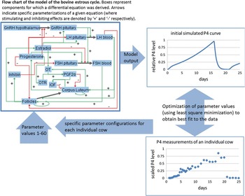
We used the deterministic mathematical model of the bovine estrous cycle originally described by Boer et al. (Reference Boer, Röblitz, Stötzel, Veerkamp, Kemp and Woelders2011a and Reference Boer, Stötzel, Röblitz, Deuflhard, Veerkamp and Woelders2011b) with the modifications introduced more recently by Stötzel et al. (Reference Stötzel, Plöntzke, Heuwieser and Röblitz2012). A schematic representation of the model is shown in Figure 1. The model describes the dynamics of the bovine estrous cycle as a set of 15 linked differential equations with 60 parameters. The differential equations describe processes of synthesis, release, and clearance of hormones and other factors, and the increase (growth) and decrease (regression) of follicle- and CL sizes. Because the exact mechanisms are often not known or more specific than necessary, so-called Hill functions are used to describe non-linear dependencies on other factors. A Hill function is a sigmoidal function between 0 and 1, which switches at a specified threshold from one level to the other with a specified steepness. The differential equations and the Hill functions are shown in Supplementary Tables S1 and S2, respectively. A complete list of parameters and their descriptions is given in Supplementary Tables S3 and S4. The initial parameterization of this model (Boer et al., Reference Boer, Veerkamp, Beerda and Woelders2012; also presented here in Supplementary Table S3), results in estrous cycles with three waves of follicular development. A complete overview of all equations and initial parameter values can also be found in Boer et al. (Reference Boer, Veerkamp, Beerda and Woelders2012) and online (http://www.ebi.ac.uk/biomodels-main/BIOMD0000000481) in SBML (Systems Biology Markup Language) code.
Overview of the iterative process of parameter fitting, illustrated with progesterone (P4) profile. Besides P4, data for luteinizing hormone (LH), follicle stimulating hormone (FSH), estradiol (E2), follicle size and corpus luteum (CL) size are simultaneously included in the least squares procedure used to fit a subset of the parameters.

Experimental data
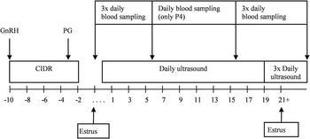
Estrous cycle-related physiological measures of cows with similar proportions of Holstein genetics, similar genetic merit for milk production traits, but with good (Fert+) or poor (Fert−) genetic merit for fertility traits (Cummins et al., Reference Cummins, Lonergan, Evans and Butler2012) were used. Good genetic merit for fertility involves a negative estimated breeding value (EBV) for calving interval and a positive EBV for cow survival, according to the Economic Breeding Index in Ireland. In total, 31 cows (19 Fert+ and 12 Fert−) had a synchronized estrus, and underwent daily ultrasonography during the cycle that followed directly after the synchronized estrus. Of the 19 Fert+ cows, 15 cows had a cycle with two follicular waves and four cows had three or more waves. Of the 12 Fert− cows, five cows had a cycle with two waves, six cows had three or more waves, and for one cow the number of waves was unknown. In total, for the 30 cows with known number of waves, there were 20 two-wave cows, five three-wave cows, four four-wave cows, and one five-wave cow. Blood sampling was carried out at 8 h intervals from day 0 to day 6 of the cycle and from day 15 to ovulation, and once daily from day 7 to day 15. Daily blood samples were analyzed for the plasma concentrations of progesterone (P4) during the entire cycle, of estradiol (E2) and FSH from day 0 to day 6 and from day 15 until ovulation, and of LH from day 15 until ovulation (Figure 2).
Synchronization protocol, blood sampling and ultrasound frequency for one complete estrous cycle relative to day of ovulation (day 0). CIDR=intravaginal progesterone (P4)-releasing device containing 1.38 g of P4; GnRH=GnRH agonist injections contained 10 µg buserelin; PG=prostaglandin F2α analogue (adapted from Cummins et al., Reference Cummins, Lonergan, Evans and Butler2012).

Processing of the data
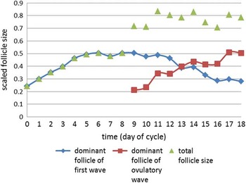
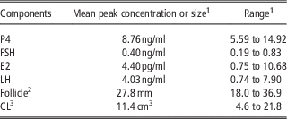
The software package BioPARKIN (Dierkes et al., Reference Dierkes, Röblitz, Wade and Deuflhard2013) was used to fit the model parameter values such that the simulations match the given data. Before importing the data files for each individual cow in BioPARKIN, the empirical data were ‘scaled’. The original model parameterization (Boer et al., Reference Boer, Veerkamp, Beerda and Woelders2012; Table S3) leads to dimensionless simulations on a relative scale, and therefore by default results in output curves between 0 and 1. However, the empirical values can lie far outside the range of 0 to 1, and can vary widely between cows. Therefore, the empirical data for each individual cow were first scaled. The measured concentrations of P4, E2, FSH and LH were scaled by dividing the concentrations by the mean peak concentration of all cows for the respective hormones (Table 1). This resulted in peak values around 1 for all cows. Thus, the scaled empirical hormone concentrations lie in the same order of magnitude as the simulated curve obtained with the initial model parameterization, but still represent the variation between cows. Data from one cow was excluded from the calculation of the mean peak hormone concentrations because she became anestrous and had undetectable or baseline P4 and E2 concentrations throughout the synchronized estrous cycle. Mean peak height of the LH surge of the cows was based on data from only 26 cows, as for four cows the LH peak could not be recognized. These four cows belonged to the Fert− group. A similar scaling procedure was followed for the CL volume and follicle diameter. The volumes of the first and second CL were calculated from their diameter (assuming a sphere). If a CL had a cavity, the cavity volume was subtracted from the CL volume. The sum of the volume of the CLs was taken as ‘CL volume’. The diameters of the dominant follicles (new and regressing) on each day were summed to give a single curve for the follicle diameter (Figure 3), which was required because follicular endocrine activity in the model is represented by continuous functions for E2 and inhibin (Inh) production, respectively. This approach assumes that the dominant follicles are the main producers of E2 and Inh (Kaneko et al., Reference Kaneko, Kishi, Watanabe, Taya, Sasamoto and Hasegawa1995; Boer et al., Reference Boer, Stötzel, Röblitz, Deuflhard, Veerkamp and Woelders2011b). To scale these follicle data, the summed follicle diameters per cow were divided by the mean peak value of the summed diameters. Data from one cow was excluded from calculation of the mean follicle diameter because the number of follicular waves could not be clearly recognized. Supplementary Figure S1 shows an example of the scaled data points for an individual cow.
Example of empirical data for the (dominant) follicle of an estrous cycle with two waves of follicular development imported in BioPARKIN. The scaled diameters of the two dominant follicles were summed to obtain total follicle diameter, and model parameter values were fitted on the resulting data points.

Mean peak hormone concentration of blood plasma or mean peak size of follicle and corpus luteum (CL) of the cows

P4=progesterone; FSH=follicle stimulating hormone; E2=estradiol; LH=luteinizing hormone.
These means are used to scale the empirical data to be in line with the initial simulated curves on a relative scale.
1 Means and range of 30 cows, except for LH (only measured in 26 cows).
2 Diameters of dominant follicles added together.
3 Summed volume of the CLs.
Parameter selection
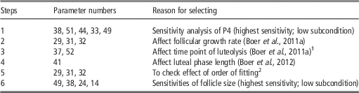
A total of 11 parameters were selected and fitted for individual cows in four consecutive steps. The previously published initial parameter values (Boer et al., Reference Boer, Veerkamp, Beerda and Woelders2012; Table S3) were the starting point for all 60 parameters. In each next step, the estimated values of the parameters fitted in the previous step(s) were used in the models for the individual cows. In the first fitting step, parameters were selected on the basis of sensitivity analysis. A general sensitivity analysis was performed to identify the time point in the cycle when the sensitivities of P4 to the 60-model parameters were highest. The five parameters with highest sensitivities and a low subcondition (Dierkes et al., Reference Dierkes, Röblitz, Wade and Deuflhard2013) at this time point were selected for the first step of parameter fitting. The subcondition is a quantity that is calculated from the sensitivity matrix in the software package BioPARKIN (Dierkes et al., Reference Dierkes, Röblitz, Wade and Deuflhard2013), and is used for rank decision in the optimization algorithm. It indicates whether or not a parameter can be estimated from the given data and thus gives some information about the dependency of a parameter on other parameters (Dierkes et al., Reference Dierkes, Röblitz, Wade and Deuflhard2013). A high sensitivity means that changes of that parameter have a large influence on P4. In contrast, parameters to which sensitivity is very low have only a small influence on the model solution and are therefore difficult to estimate.
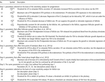
For fitting steps 2, 3 and 4, another six parameters were selected that were previously reported to play an important role in the model in regulating follicular wave pattern (Boer et al., Reference Boer, Röblitz, Stötzel, Veerkamp, Kemp and Woelders2011a) and P4 profiles (Boer et al., Reference Boer, Veerkamp, Beerda and Woelders2012). Table 2 shows the order of fitting steps and the rationale for selecting the parameters. Table 3 provides a description of the 11 fitted parameters. A more elaborate description of all parameters is given in Supplementary Table S4. Two more fitting steps were run as extra tests. First, the effect of the order of fitting the parameters was investigated by performing step 2 (parameters 29, 31 and 32) without first performing step 1 (i.e. starting with the initial parameterization). Second, starting again with the initial parameterization, a sensitivity analysis for the sensitivity of follicle size to variation of each parameter was performed, and the parameters with high sensitivity and low subcondition (parameters 49, 38, 24 and 14) were fitted (fitting step 6).
Selection of parameters to be fitted in a series of fitting steps

1 Parameters identified in Boer et al. (Reference Boer, Röblitz, Stötzel, Veerkamp, Kemp and Woelders2011a) to affect time point of luteolysis would in the present model translate to par 37, 51 and 52. But parameter 51 was already fitted in the first fitting step.
2 Fitting parameters 29, 31 and 32 (step 2) without first performing step 1.
Model parameters selected for value estimation for each individual cow in four consecutive steps

CL=corpus luteum; Foll=follicle size; FSH=follicle stimulating hormone; Inh=inhibin; IOF=intra ovarian factors; OT=oxytocin; OTR=oxytocin receptor; P4=progesterone; PGF2α=prostaglandin F2 alpha.
Parameter identification
Model parameter values were fitted in the software package BioPARKIN (Dierkes et al., Reference Dierkes, Röblitz, Wade and Deuflhard2013) to obtain closest agreement between model output and empirical data points for each cow, using a least squares optimization procedure (Dierkes et al. Reference Dierkes, Röblitz, Wade and Deuflhard2013). To restrict the parameter space and thus facilitate optimization, the parameter ranges were constrained to 10-fold the initial value. As the least squares method analyzes the ‘vertical distances’ between simulated and empirical data (i.e. not across time), time shifting was applied to the data that resulted in an optimal overlap between the initial curves and the imported data in order to obtain the best initial guess in fitting the curves. Curves simulated by the model were visually assessed for agreement with empirical endocrine profiles and the number of follicular waves and other estrous cycle characteristics. Mean parameter values were compared between cycles with different numbers of waves, and between cycles in cows with low and high genetic merit for fertility (Fert+ or Fert−), using a t-test. With the new estimated values of the 11 fitted parameters in the model, a new sensitivity analysis was performed for each cow to see whether the order of sensitivities and subconditions was changed. An overview of the iterative process of parameter estimation is shown in Figure 1.
Results
Sensitivity analysis
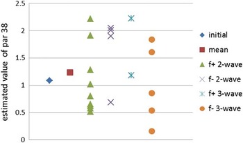
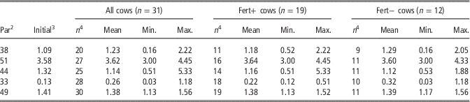
The general sensitivity analysis of the model with the initial model parameterization showed that P4 is most sensitive to parameter changes around the time point of onset of luteolysis at day 16.3 (Supplementary Figure S2). The 10 parameters to which P4 was most sensitive were the same as the parameters to which the CL volume was most sensitive. Of these 10 parameters, five parameters (parameter 38, 51, 44, 33 and 49) had a low subcondition and were fitted in the first fitting step. Parameter 38, 51 and 44 are involved in luteolysis, parameter 33 affects follicle size, and parameter 49 is involved in Ihn production. A description of these five and the other fitted parameters is given in Table 3 and Supplementary Table S2. The estimated values for these five parameters varied between cows, especially parameter 38 (Figure 4) and parameter 33 Table 4). Remarkably, the mean, minimum and maximum estimated parameter values were similar for the cows with good (Fert+) and the cows with poor EBV for fertility (Fert−), with no significant differences between the two groups. For parameters 33 and 38, the variation in estimated values was larger in the group of Fert− cows compared with the Fert+ cows.
Estimated values per cow for parameter 38 in fitting step 1. Parameter 38 is the oxytocin threshold concentration in the model for stimulation of prostaglandin F2α (PGF2α) secretion in the uterus. Initial= initial parameter value; mean= mean of estimated (fitted) values; f+=‘Fert+’ group; cows with good estimated breeding value (EBV) for fertility; f−=‘Fert−’ group; cows with poor EBV for fertility; 2-wave=two waves of follicular development per cycle; 3-wave=three or more follicular waves per cycle.

Means and ranges of estimated parameter values for parameters with low subcondition and to which progesterone (P4) had a high sensitivity (fitting step 1); the other parameters remained fixedFootnote 1

Fert+=good genetic merit for fertility traits; Fert−=poor genetic merit for fertility traits.
1 All other parameters remained at the initial values of the original model.
2 Parameter number.
3 Initial value of the original model.
4 Number of cows for which the respective parameter could be estimated.
Follicular wave pattern
In each of the following fitting steps 2, 3 and 4, the parameters fitted in the previous step(s) were set to the values obtained for the individual cows, whereas the other parameters remained at the initial value. A description of the six parameters fitted in these steps is given in Table 3 and Supplementary Table S2. In step 2 of fitting, parameters 29, 31 and 32 were fitted simultaneously. In a previous study, the model (Boer et al., Reference Boer, Röblitz, Stötzel, Veerkamp, Kemp and Woelders2011a) parameters 29, 31 and 32 were found to affect the number of follicular waves via changes in follicular growth rate. The highest variation among cows in estimated parameter value was found for parameter 31 (Table 5). There was no significant difference in estimated values for these parameters between cows that had a cycle with two waves or cows that had a cycle with three or more waves of follicular development. Applying the newly found parameter values for the individual cows also did not give a substantial change in the simulated follicular wave pattern. In step 3 of fitting, parameters 37 and 52 were fitted simultaneously. The study of Boer et al. (Reference Boer, Röblitz, Stötzel, Veerkamp, Kemp and Woelders2011a) showed that the number of waves was not only affected by follicle growth rate but also by time point of luteolysis. The modeling of luteolysis in Boer et al. (Reference Boer, Röblitz, Stötzel, Veerkamp, Kemp and Woelders2011a) had been slightly different from the current study, but the wave pattern effects identified by Boer et al. (Reference Boer, Röblitz, Stötzel, Veerkamp, Kemp and Woelders2011a) relate in the present model to parameters 37, 51 and 52, but parameter 51 was already fitted in the first step. The estimated value for parameter 52 appeared to be lower for cows with two waves than for cows with three or more waves (Table 6), but the difference was not significant. In step 4 of fitting, parameter 41 was fitted. In a previous study, parameter 41 had been shown to have a large effect on luteal phase length (Boer et al., Reference Boer, Veerkamp, Beerda and Woelders2012). The now obtained estimated values for parameter 41 were all very close to the initial value of 0.04. The effect of the order of fitting the parameters was investigated by performing step 2 (fitting parameters 29, 31 and 32) without first performing step 1 (i.e. starting with the initial parameterization). This resulted in almost similar parameter values for these three parameters, but poorer performance regarding the predicted number of follicular waves.
Means and ranges of estimated values of three parameters reported to affect follicular growth rate (fitting step 2); the other parameters remained fixedFootnote 1

1 Estimated values for individual cows were used for the parameters presented in Table 4. All other parameters remained at the initial values of the original model.
2 Numbers between brackets are the number of cows for which the parameter values could be estimated out of the total number of cows in that group.
3 Parameter number.
4 Initial value of the original model.
Means and ranges of estimated parameter values of two parameters reported to affect time point of luteolysis (fitting step 3); the other parameters remained fixedFootnote 1

1 Estimated values for individual cows were used for the parameters presented in Tables 4 and 5. All other parameters remained at the initial values of the original model.
2 Numbers between brackets are the number of cows for which the parameter values could be estimated out of the total number of cows in that group.
3 Parameter number.
4 Initial value of the original model.
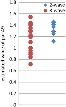
In above four-step fitting, in the first step, parameters had been selected to which P4 concentration was most sensitive, but the sensitivities strongly depended on the time point in the cycle. Therefore, we compared fitting of parameters selected on the basis of the sensitivity of follicle size (instead of P4). The sensitivities of follicle size to each parameter was calculated (using the model with initial parameterization). Now, parameters 49, 38, 24 and 14 had highest sensitivities and low subcondition and were fitted (keeping all other parameters fixed on their initial values). Note that parameters 49 and 38 had also been fitted in step 1 of the four-step fitting described above, as they had high sensitivity and low subcondition for both follicle size and P4. The now estimated parameter values of parameters 49 and 38 differed strongly among cows, but applying the estimated parameter values to the model did not result in an altered wave pattern or altered peak values for follicle size. However, interestingly, the estimated value for parameter 49 (proportionality constant for Inh secretion by the follicles) was significantly lower for cows with three or more waves of follicular development per cycle compared with cows with two waves (Figure 5), despite the fact that the distribution of the three-wave cows overlaps the distribution of the two-wave cows.
Estimated values per cow for parameter 49 in fitting step 6. Parameter 49 is the proportionality constant in the model for inhibin secretion by the follicles. Inhibin suppresses follicular growth via inhibition of FSH synthesis in the pituitary. Estimated parameter values for cows with two waves (two-wave) and cows with three or more waves (three-wave) of follicular development per cycle.

Performance of the model with the new values for the 11 fitted parameters
After fitting the total of 11 parameters in steps 1, 2, 3 and 4, a new sensitivity analysis was performed with the estimated values for the fitted parameters in the model for each cow. Now, an additional parameter, parameter 41, was found to which P4 has a high sensitivity. Parameter 41 now ranked among the 10 most sensitive parameters for 12 cows, which was not the case when using the initial parameterization. For 11 of these 12 cows, a clear change in the number of follicular waves was observed when using the estimated values for the 11 fitted parameters compared with the model with the initial parameterization. The estimated value of parameter 41, however, shows very little variation between cows. In this second sensitivity analysis parameters 18, 23, 55, 58 and 60 had a low subcondition for a number of cows, but sensitivity of P4 to these parameters was not very high.
Compared with the initial parameterization, the simulated follicular wave pattern had changed for 21 cows when using the new values for the 11 fitted parameters. The initial parameterization gives an estrous cycle with three follicular waves. But in the empirical data, there were 20 cows with a two-wave cycle. With the new parameter values the model had correctly ‘switched’ from a three-wave to a two-wave cycle for 13 of these 20 cows. For eight of the 10 cows with three or more waves, the model predicted a three-wave cycle. The number of predicted waves was correct for all five cows that had a three-wave cycle. For the four cows that had four waves, the model predicted a three-wave cycle for three cows, and an irregular pattern was predicted for the fourth cow. So in total, the new parameterization led to an improved follicular wave pattern (in terms of wave number and/or visual match with the empirical data) for 18 of the 21 cows for which the wave pattern had changed from that of the initial model, and the number of follicular waves was predicted correctly for 18 of the 25 two-wave and three-wave cows.
In two of the three-wave cows, the third follicular wave of the simulated cycle started before the second wave was finished (i.e. the continuous function for follicle size had not gone down much after the second wave) (Supplementary Figure S3), in agreement with the fact that in the empirical data the newly arising and the regressing follicles overlapped. A similar ‘intermediate’ pattern between two-wave and three-wave cycles was also predicted for four of the 20 cows with a two-wave cycle. For 13 of the 20 cows with a two-wave cycle, a two-wave cycle was predicted for the simulated cycle in which the empirical data was overlaid (Supplementary Figure S4) or for the subsequent simulated cycle (Supplementary Figure S5).
Discussion
In the current study, a mechanistic mathematical model of the bovine estrous cycle was parameterized for an independent data set comprising measurements of 31 individual cows. The main objective of this study was to further validate this model by investigating whether the model is able to accommodate normal variation in estrous cycle characteristics of individual cows, using the empirical data of measured hormone profiles and follicle and CL sizes in 31 individual cows with different genetic merit for fertility. Previous successful validation steps were (1) creating a parameter configuration (a specific combination of parameter values for the set of model parameters) that can simulate an ‘average’ normal cycling cow (Boer et al., Reference Boer, Röblitz, Stötzel, Veerkamp, Kemp and Woelders2011a), (2) creating parameter configurations that can simulate various physiological settings, using different approaches (Boer et al., Reference Boer, Stötzel, Röblitz, Deuflhard, Veerkamp and Woelders2011b and Reference Boer, Veerkamp, Beerda and Woelders2012) and (3) simulating estrous cycle synchronization protocols based on PGF2α administration (Stötzel et al., Reference Stötzel, Plöntzke, Heuwieser and Röblitz2012). In the current study, it was investigated whether the model is able to find parameter configurations for 31 individual cows without taking extreme, probably non-physiological values. Martin et al. (Reference Martin, Friggens, Dupont, Salvetti, Freret, Rame, Elis, Gatien, Disenhaus and Blanc2013) defined data-derived profiles for LH, FSH, E2 and P4, which are useful for benchmarking normal dynamics of reproductive hormones. Our current study contributes to defining such reference profiles, but also addresses hormone profile and follicular wave variation between individuals. This can help to explain differences between reference profiles and individual measurements and to predict how reference profiles can be disturbed, which ultimately can help to find biological mechanisms that could induce reproductive problems.
Approach of parameter estimation
This study started with a sensitivity analysis to identify the parameters to which P4 concentrations are most sensitive, and to find how the sensitivities changed during the cycle. Also, the sensitivity analysis gives a ranking of subconditions, which provides a measure of the dependency of a parameter on other parameters. Parameters with a high sensitivity at the onset of luteolysis and with a low subcondition were fitted first because these were assumed to have a major effect on the bovine estrous cycle, and to be independent from other parameters. The ranking of the parameters in the sensitivity analysis depends on the chosen conditions. First of all, sensitivities, may depend on the time point of the cycle, which indeed was seen for the sensitivities of P4. However, calculating sensitivities for another component (Follicle size instead of P4) did not result in highly different parameter values. Second, the sensitivities (and subconditions) may become different when a different parameterization is used. In that case, other parameters could be selected to be fitted first, resulting in a different order of parameter estimation. The use of the same approach for each cow in this study (i.e. fitting the same parameters in the same order for each cow), allowed comparison of the results with each other. Furthermore, fitting a subset of parameters (parameter 29, 31 and 32) in another order (i.e. before or following fitting parameters 38, 51, 44, 33, 49) did not result in major differences in the estimated values.
The first five parameters were fitted one by one (and not simultaneously). This can be successful as indeed the selected parameters had a low subcondition (i.e. they were less dependent on other parameters). Parameters were fitted simultaneously in the subsets of parameters of fitting steps 2 and 3, respectively. It is difficult to fit (larger) parameter sets together due to the dependencies within the model. The sensitivity analysis gives an order of subconditions and thus a hint of parameter combinations that are promising to be successfully fitted together. However, subconditions change as parameter values change during the consecutive fitting steps. As a priori information, the subcondition thus has to be taken with caution. To improve this issue of finding appropriate parameter combinations, it is also helpful to take into account known biological mechanisms when deciding on which (combinations of) parameters to fit. Manually changing parameter values and assessing its effect on the predicted endocrine profiles can support this decision. Whether or not parameters can be estimated together may provide insight into dependencies between model mechanisms, and thus elucidate potential interactions in the biological system of bovine estrous cycle regulation. Parameter value sets that optimally fit the data are not necessarily unique. Therefore, conclusions to their optimality from a biological point of view need to be drawn with caution. Some parameters can compensate or depend on other parameters and thereby cause some ‘arbitrariness’ in their absolute value. This relates to the problem of identifiability as different (combinations of) parameter values may be equally consistent with the data (Fernández Slezak et al., Reference Fernández Slezak, Suárez, Cecchi, Marshall and Stolovitzky2010).
Biological relevance of inter-individual variation of parameter values
For most parameters, the estimated values varied between the individual cows. Variation in estimated values for a parameter could indicate that this parameter explains biological differences between cows. However, such variation may also reflect low sensitivity of the system to that parameter. This may be interpreted as ‘robustness’ of the system; the parameter value can vary without loss of biological function. Parameters to which the output (e.g. P4) has a high sensitivity and which have high variation in estimated value could be interesting because they could explain differences in estrous cycle characteristics between individual cows. But also parameters with a small variation in estimated values can be interesting, provided that the sensitivity is very high, as this would indicate that only a small variation is sufficient to obtain a good fit.
If the variation in parameter values is high in the sense that some cows strongly deviate from the average cow, these cows have apparently a deviating regulation of the estrous cycle, which could be indicative of suboptimal cyclicity and fertility. When estimated parameter values for different cows are closer together, as is the case in the Fert+ group, this could mean that the optimal (combination of) values have been found for this group of cows. Therefore, these values might be fixed when performing optimization of subsequent parameters. The highest value in an animal for parameter 33 (threshold for P4 to stimulate decrease of follicle size) was relatively extreme (compared with the mean and variation in the other cows) and belongs to the one cow in the data set with five follicular waves. This is not surprising, as a high value of parameter 33 will result in a lower inhibitory effect of P4 on follicular growth. The effect of P4 on follicular growth (partly represented by parameter 33), together with the effect of Inh (partly represented by parameter 49), affect the time point and rate of regression of the dominant follicle of a wave. The highest value for parameter 44 (threshold for inter ovarian factors to stimulate CL regression) was an outlier belonging to a cow with high P4 concentrations for a number of days after the relatively large CL started to regress. It is therefore not surprising that for this cow a deviating value was found for this parameter 44 involved in luteolysis. These outliers confirm model behavior in deviating physiological settings and are thereby helpful for validation of the model.
Model performance
This study showed that the model of the bovine estrous cycle can be parameterized to fit the empirical data of individual cows. For most parameters, the resulting estimated values differed from the initial starting values. For instance, the mean estimated value for parameter 33 (threshold for P4 to stimulate decrease of follicle size) was twice as high as the initial value. In addition, the estimated parameter values varied between the individual cows. However, there were no clear differences in estimated values for specific parameters when comparing the groups of cows. The Fert+ cows had significantly higher peripheral blood P4 concentrations than the Fert− cows (Cummins et al., Reference Cummins, Lonergan, Evans and Butler2012). In addition, the Fert+ cows tended to have fewer follicular waves than the Fert− cows. The parameters fitted in step 1 may be expected to affect the follicular wave pattern through effects on luteal phase length or follicle growth rate (parameters 38, 51 and 44 are involved in luteolysis, parameter 33 affects follicular function, and parameter 49 is involved in Inh production). But no (significant) differences in the estimated values for these parameters were found between the Fert+ and Fert− cows, although the variation between cows within the groups appeared to be larger in the Fert− group. In fitting steps 2, 3 and 4, there were also no differences between the cows with two waves v. cows with three or more waves. In step 3, the estimated value for parameter 52 appeared to be lower for two-wave cows compared with cows with three or more waves, but the difference was not significant. In addition, in step 4, parameter 41 (maximum rate of increase of CL stimulated by itself), which in a previous study had a large effect on luteal phase length (Boer et al., Reference Boer, Veerkamp, Beerda and Woelders2012), and thus could affect the number of waves per cycle, had estimated values for all cows very close to the initial value of 0.04. This suggests that, in the current settings, parameter 41 does not explain differences in luteal phase length. However, it could be that luteolysis (e.g. CL regression) has a high sensitivity to parameter 41, which would mean that small variations could change the model behavior. The results did suggest a role for parameter 49 (proportionality constant for Inh secretion by the follicles) in the follicular wave pattern, as the estimated value for parameter 49 was significantly lower for cows with three or more waves of follicular development per cycle compared with cows with two waves. However, the fact that the distribution of parameter values for parameter 49 overlapped for the three-wave and the two-wave cows indicates that the number of follicular waves (two- or three-wave pattern) is determined by other parameters as well.
Despite the fact that there were no clear associations between estimated values for individual parameters and the number of waves per cycle of the cows, the model was able to simulate the empirical data and to correctly predict the number of follicular waves per cycle of most cows. The initial parameterization of the model results in a default three-wave cycle, whereas in the empirical data there were 20 cows with a two-wave cycle. When applying the new estimated values of the fitted parameters to the model, the model behavior changed for 21 cows, and the number of follicular waves was predicted correctly for 18 of the 25 two-wave and three-wave cows.
It could be that a change in output curves is induced by small changes in several parameters together, or that different configurations (specific combinations of parameter values for the set of model parameters) can lead to a similar phenotypic output. For instance, if a two-wave cycle can result with widely different settings of a specific parameter, but in combination with a number of other parameters the total setting generates a two-wave cycle. In the reality of biological systems it is likely that a perturbation is the effect of simultaneous changes in multiple physiological parameters, as can be simulated in the model by multi-parameter perturbations (Boer et al., Reference Boer, Veerkamp, Beerda and Woelders2012). In the current study, the predicted peak CL volume was not always well adapted to the data points (e.g. Supplementary Figures S6 and S7), even though the order in which the parameters where estimated was based on P4 sensitivities, and therefore indirectly on CL sensitivities. Parameter identification was thus not very successful in predicting the variation in peak CL volume, although such variation clearly existed in the raw data. This lack of variation could be due to a suboptimal (combination of) parameters that were fitted, which would also point to the importance to find the appropriate combinations of parameters to be estimated simultaneously.
Parameter identification was not successful for four-wave cycles, possibly due to the way the follicle data are processed in the model. However, a previous study with the model (Boer et al., Reference Boer, Veerkamp, Beerda and Woelders2012) showed that the model can simulate cycles with four or more follicular waves. Due to the way follicular function is represented in our model, separate follicular waves can be distinguished, but separate follicles are not. Due to the overlap of subsequent follicles (in empirical data), the total summed follicle size may not show a clear wave pattern, although obviously there is growth and regression of dominant follicles. Improving the prediction of follicle size could be done in two ways. The first way is by processing the empirical data, such that the separate follicular waves can be more easily distinguished. The second way is by changing the way that follicle size is represented in the model. For instance by modeling each follicle separately, as was done by Bondouy and Röblitz (Reference Bondouy and Röblitz2012), although that method does yet not account for the fact that in experimental data a regressing follicle from a previous wave is still visible as a structure. In addition, further development of the model could consist of including an extra equation (with Hill function) to distinguish functional and structural follicular development. Increased steroid clearance has been suggested as a potential mechanism responsible for reduced circulating P4 concentrations in lactating dairy cows (Wiltbank et al., Reference Wiltbank, Lopez, Sartori, Sangsritavong and Gumen2006). For future work, it would therefore be interesting to fit the model parameters of ‘P4 clearance rate’ and ‘proportionality factor of CL in P4 increase’ together. Similarly, the proportionality factor for E2 secretion and the clearance rate for E2 could be fitted to investigate whether increased steroid clearance or follicular E2 synthesis can explain variation between animals in peripheral blood P4 and E2 concentrations.
Conclusions
This study showed that the model of the bovine estrous cycle can not only be parameterized to simulate an ‘average’ cow, but also estrous cycles of individual cows on the basis of their ‘real’ estrous cycle data, without taking extreme, probably non-physiological parameter values. The model is able to accommodate normal variation in estrous cycle characteristics, using the empirical data of measured hormone profiles and follicle and CL sizes in individual cows. Thus indications of possible differences between cows in the underlying processes related to the model parameters can be obtained. Although it was difficult to detect significant differences in values for specific single parameters between groups with different estrous cycle characteristics, the results of this study indicated that certain combinations of estimated parameter values induce a clear qualitative change in model behavior (e.g. a different number of follicular waves or a change in peak hormone concentrations). This suggests that external or genetic influences on estrous cycle characteristics may have their effect via the mechanisms regulated by these parameters. In conclusion, in this study we validated the mathematical model of the bovine estrous cycle by demonstrating its ability to accommodate experimental data from individual cows. Further, this study is a first step toward finding specific parameter configurations (specific combinations of parameter values for the set of model parameters) that could explain differences in follicular growth and endocrine concentrations between cows. Thus, the mathematical model can be used as a tool to predict biological mechanisms underlying differences in the estrous cycle between dairy cows.
Acknowledgments
Thanks to Prof. Dr B. Kemp and Dr B. Beerda for their useful comments on the manuscript. Dr T Dierkes is acknowledged for his technical assistance with BioPARKIN, and Dr S. Röblitz for the provided support. The research leading to these results has received funding from the European Union Seventh Framework Programme (FP7/ 2007-2013) under the grant agreement no. 311776. C.S. has been supported by the DFG Research Center MATHEON ‘Mathematics for Key Technologies’ in Berlin, Germany.
Supplementary material
To view supplementary material for this article, please visit https://doi.org/10.1017/S175173111700026X