


1. Introduction
The actual management of natural resources and ecosystems inspires great concerns about sustainability and welfare. Notably, the possible depletion of shared stocks, and the dumping of harmful pollutants into commons, cause worries about efficiency, equity, and legitimacy.
Typically, the related industries must make heavy investments up front that cannot easily be recouped later on. Also, the net returns may appear rather uncertain in magnitude and distant in time. Together these facts beg for thorough investment analysis, emphasizing precaution and the value of keeping options alive.
For such analysis several disciplines have much to offer. First comes the economics of finance and insurance. Further, since practical planning cannot avoid computation altogether, there is, in principle, no escape from simulation and optimization. Also, because exchange is implicit or lurking in the background, so-called production or market games can elucidate multi-agent interaction.
It is seldom though, that all these ingredients are found in one and the same study. Most analysts contend with the restricted perspective – and the partial analysis – that suits a single agent, situated within well-defined markets. Easily ignored then is the endogenous nature of allocations and prices. And even more troublesome is absence of markets for some inputs, products, or risks. Their absence greatly affects the willingness to invest in irreversible, large-scale projects that have unpredictable and remote payoffs.
Projects of precisely that sort are the objects of this paper. Each offers uncertain returns, and each is owned by a separate agent who acts as investor and producer. Our main interest revolves around the total and marginal value of investing in those projects. As will become clear, such values are interdependent, subject to contingencies, and jointly determined. Planning is therefore faced with the problem of coordinated portfolio choice. Especially interesting are papers or projects that swing out of phase – or aren't quite aligned – with others. Examples of such sort abound. Included are:
• selective gear for harvesting multi-species, multi-cohort fish stocks;
• diversification over crops, livestocks, and ecological orientations in agriculture;
• alternative energy, generated by biomass, sunshine or wind. In each case, the technology is costlier to install or operate, but better at safeguarding the environment.
For more concrete examples, consider two arrangements for electricity generation. In the first, suppose all plants are driven by hydro-power. Some plants depend on highly correlated, short-term precipitation. They are well furnished in chilly, wet years. Other, more expensive plants merely tap melting water from under a glacier. They are best off in dry, warm years. Given aggregate supply commitments, the two groups of producers can mutually insure each other. Such insurance ex post affects investments ex ante.
In the second arrangement, suppose the base load is delivered by thermal or nuclear plants. Hydro-power then acts merely as swing producer. By serving peak demand it receives higher price. Again, prudent investments require a sector-wide perspective – or well-functioning markets (Flåm and Gassmann, Reference Flåm, Gassmann, Marti, Ermoliev, Makowski and Pflug2006).
To study such instances section 2 introduces the prototypical agent. Section 3 places several of them into a two-stage, cooperative setting, affected by much uncertainty. Brought out there are core solutions ex ante and ex post, both determined by shadow prices. Section 4 offers some novel qualitative results, akin to covariance-pricing in finance. Section 5 illustrates a few insights about parallel projects, and section 6 briefly discusses comparative risk advantages. Section 7 considers attainment of equilibrium in environmental games, and section 8 concludes.
This paper addresses at least three types of readers. Included are: first, economists, not quite aware of the rich opportunities production games offer; second, finance or insurance analysts, rarely concerned with Lagrangian duality; and, third, optimizers, not fully conversant with the cooperative aspects of such duality.
2. The risk-exposed agent
This section introduces the prototypical agent. He acts in two roles: as investor and producer. Whether he operates alone or in a consortium, his actions and decisions evolve step-wise, in a sequence described next:

The upper bound k reflects an established limit or property right.Footnote 1 Examples are manifold. The table below indicates some instances:

In any case, the realization ω remains unknown at the time when k is chosen. By contrast, Δk, r, q are contingent decisions, depending on the pair (k, ω).
At this point two modelling issues come up. The first concerns dimensionality, the second uncertainty. Regarding the first, we may easily accommodate several sorts of capacities, resources, and products, increasing thereby the dimension of the decision spaces. Doing so entails, in principle, no additional complexity, be it in analysis or presentation (albeit of course in computation).Footnote 2 In fact, the reader may choose freely whether to regard some items as vectors or real numbers. It helps intuition though, to deal merely with one-dimensional spaces.
The second modelling issue concerns perception of risk and uncertainty. Such matters bear, of course, on what is known, unknown, or unknowable (Gomory, Reference Gomory1995). We take a traditional stand here by assuming that uncertainty amounts to a probabilistic description of possible outcomes ω ∈ Ω. Further, we may posit that the probability distribution of ω be identified by each and every concerned party. This hypothesis is certainly convenient, but hardly realistic. For a distribution-free approach we must contend with sequential realizations of ω one after the other, and the attending build-up of empirical statistics – possibly path-dependent. We shall deal with both settings. In either, E denotes the expectation operator with respect to ω. To bypass purely technical concerns about measurability and integrability, assume Ω finite. Several sorts of uncertainty may prevail, be it in preferences, productivity, or resource abundance.
While still facing uncertainty, the prototypical agent wants to maximize the expectation of his payoff. Thus, if operating in autarky, isolated from others, he should

Here and elsewhere we do not mention evident sign restrictions such as k, r, q ≥ 0. Note that problem (1) has two stages. First, k must be sunk before knowing ω. Second, after ω and e(ω) are unveiled, the subsequent decision (Δk, r, q) had better

Format (1) is generic and quite general, able to accommodate manifold instances. In particular, if capital adjustment comes at prohibitive cost, Δk is not mentioned. Similarly, when e is lacking, r disappears.
The subsequent section introduces several such agents, each willing to accept side payments. Moreover, at least some privately owned item is transferable – be it a capacity, endowment, resource, or output. The agents may gain therefore, by abandoning extreme individualism and self-sufficiency. Instead of everybody going alone, they could coordinate their enterprises as described next.
3. Stochastic production games
Accommodated henceforth is a fixed, finite set I of agents, each of the prototypical sort just described. Agent i ∈ I proceeds step-wise, in the following order:
First, he installs capacity k i ≤ k i. Next, he observes the actual state ω and his endowment ei(ω).
Thereafter, he makes capital adjustment Δki, uses resource ri, and produces output f i(k i ω, Δk i, r i).
Finally, it is time for him to market output quantity qi and collect payoff πi(k i, ω, Δk i, r i, q i).
At first glance, the individual problems appear decoupled – or almost autarkic. They are coupled however – and the agents interrelated – because utilities and some factors are assumed transferable. Coalitions can therefore pool resources and redistribute gains.
Formally, what the parties could – and in their own interest, ought to – play is a transferable-utility cooperative game in characteristic form. Each instance of such a game associates a value VS to coalition S ⊆ I. The most common and popular solution concept is the core (Moulin, Reference Moulin1995; Osborne and Rubinstein, Reference Osborne and Rubinstein1994; Owen, Reference Owen1982): a payment scheme (u i) ∈  I belongs to the core iff it entails

The efficiency constraint requires that the overall value VI is fully shared. The no blocking constraint captures that a dissatisfied coalition S, when offered merely ∑i∈Su i < V S, would defect.
Two value functions arise naturally here: a first one up front, a second one at the subsequent stage. At that stage, given state ω and capacity profile kS := (k i)i∈S of coalition S, that set of players can achieve ex post value

The maximum in (2) is taken with respect to (Δk i, r i, q i)i∈S. Here and henceforth, by assumption, each maximal value is attained.
Equation (2) presumes pooling and transfers of utilities, endowments, and outputs. Those operations fit fishermen, endowed with individual quotas. But it doesn't quite fit generation of hydro-electricity from non-connected basins. There, the constraints on water resources remain disaggregated; that is, r i ≤ e i (ω) for each i ∈ S. We refrain from spelling out various instances and easy modifications. What imports is that utilities and at least one commitment or factor be transferable. For simplicity, we proceed as though all items are transferable, favoring thereby fisheries as a leading example.
Ex ante the same coalition could shoot for value

Equation (3) could of course be extended to incorporate lower bounds on some capacities or treat them as already committed. Here however, to emphasize the importance of up-front investment, such details are omitted. Clearly, the values just defined, be it V S = v S (kS, ω) or V S = v S (k S), are superadditive; that is

This inequality system indicates that gains can be had by coordinating investment and production. So we ask: Can all cooperative benefits be achieved and shared?
Under some natural and standing assumptions, there is a constructive and positive answer – as will be brought out next. Those assumptions include that for each ω the contingent functions πi, fi should be concave in the other variables, and that each πi be increasing in (ri, qi).
First-stage cooperation (3) anticipates another such enterprise to follow suit at the second stage (2). It is natural therefore, to disentangle one stage from the other.
We begin with the second one. To come to grips with cooperation there, consider the grand coalition S = I, let k := kI = (k i)i ∈ I, and associate a Lagrange multiplier Λr (k, ω) to the resource constraint in (2). Associate a similar multiplier Λq(k, ω) to the quantity constraint there. When speaking of such multipliers we tacitly mean that the Lagrangian L(k, ω, Δk, r, q, λ} :=

after insertion of λ := ⌊λr, λq⌋ = ⌊Λr(k, ω), Λq (k, ω)⌋, should satisfy

Proposition 1. (Ex post contingent core solutions) Given a grand capacity profile k := (k i)i∈I, and a realization ω ∈ Ω, suppose Λr(k, ω), Λq(k, ω) are Lagrange multipliers associated to resources and quantities. Then, ex post, the state-dependent payment scheme u i(k, ω) :=

belongs to the core of the second-stage, contingent game that has the characteristic function S ↦ v S(kS, ω) defined by (2).
When ∑i∈I [e i(ω), f i(k i, ω, 0, e i (ω))] ≫ 0, there do exist Lagrange multipliers.
Still regarding the grand coalition S = I, let

be its overall Lagrangian. Again, when speaking of multipliers ω ↦ λr(ω) λq (ω), associated to the resource and quantity constraint in (2), and μ to ∑i∈Ik i ≤ ∑i∈Ik i =: k I, we mean that

Proposition 2. (Ex ante core solution) For the grand coalition suppose ω ↦ λr(ω), λq(ω) and μ are Lagrange multipliers associated to the constraints on resources, quantities, and capacities, respectively. Then the payment scheme U i(k i, ∑j≠ik j) :=
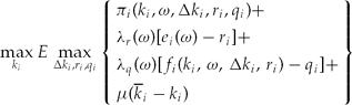
constitutes an overall core solution for the game that has the characteristic function S ↦ v S(k S) defined by (3).
If ∑i∈I ⌊e i(ω), f i(k i, ω, 0, e i(ω))⌋ ≫ 0 almost surely, and k I > 0, there do exist Lagrange multipliers ω ↦ λr(ω), λq(ω) and μ.
One should not be lured into thinking that commonplace multipliers, furnished by necessary optimality conditions for problems (2), (3), automatically generate core imputations via (6). Rather, what imports here is that assumptions (4), (5) have the nature of sufficient optimality conditions. To satisfy these it largely helps to have πi, fi concave for each ω.
A comment on externalities is in order. Individual players and problems are of course coupled by the balancing of total capacities, endowments and resources. Yet, still more coupling could come about. To wit, the aggregate parameters k I = ∑i∈Ik i and e I(ω) = ∑i∈Ie i (ω) might affect payoffs πi. If so, the preceding arguments would still hold. Of particular notice in this regard are games involving commons. Typically then, the restriction ∑i∈Ir i ≤ e I(ω) binds, and the aggregate e I(ω) – be it catch, energy supply, or pollution – affects all parties.
Taken together the above propositions, proven in the Appendix, show how agents, having convex preferences and stochastic assets, can pool inputs, outputs and endowments to smoothen and insure individual payoffs across eventualities and time (Flåm, Reference Flåm2002). Individual projects can thus share risks – and occasionally even eliminate them. In particular, this holds when parties are few and risks idiosyncratic, so that neither the law of large numbers nor the Arrow–Lind theorem apply (Arrow and Lind, Reference Arrow and Lind1970). The main instruments for risk sharing are endogenous prices. These emerge as Lagrange multipliers, and they equilibrate intrinsic markets (Shapley and Shubik, Reference Shapley and Shubik1969). At those markets all parties are construed as price-takers.
Propositions 1 and 2 relate to the welfare properties of competitive equilibrium that stem from its residence within the core. To emphasize this link is certainly useful, but not quite necessary. In fact, Shapley–Shubik's cooperative perspective on market games contends with a broader solution concept, namely the core (Shapley and Shubik, Reference Shapley and Shubik1969). Important and novel here is the presence of two stages – and associated recourse options, exercised as events unfold. Particularly interesting are differential impacts of uncertainty on various projects. We address that issue next.
4. Covariance-pricing of projects
Let  ,
 ,
 denote the recourse decisions, assumed unique and well defined, that solve (6). Write f i(k i, ω) for the resulting production
 . The two terms λre i and λqf i(k i) are in focus here. They record the reimbursements to agent i for his endowment and output respectively. To inquire about the nature of these pecuniary items, recall that two real-valued random variables X, Y are declared negatively dependent (or briefly: − dependent) if for all values x, y

Thus, there is negative dependence if Pr[X ≤ x|Y ≤ y] ≤ Pr[X ≤ x]. Broadly, knowing Y small, reduces the likelihood of X also being small. Positive dependence (briefly: + dependence) obtains when Pr[X ≤ x, Y ≤ y] ≥ Pr[X ≤ x] Pr [Y ≤ y] for all x, y.
Proposition 3. (Dependence and covariance (Magill and Quinzii, Reference Magill and Quinzii1996)) If X, Y are negatively (positively) dependent and D : → is strictly decreasing, then X, D(Y) are oppositely dependent, and the sign of cov(X, Y) is −1 (+1 respectively).
Although random, the multipliers λr and λq in (6) depend largely on the aggregate endowment eI and output f I := ∑i ∈ If i respectively. Ceteris paribus, the dependence shows up as ‘inverse demand curves’ e I ↦ λr(e I), f I ↦ λq(f I). By the ‘law of demand’ such curves tend to decrease. Not surprisingly, this property obtains here also:
Proposition 4. (Monotonicity of shadow prices) The inverse demand curves e I ↦ λr(e I), f I ↦ λq(f I) are both decreasing. That is, it holds almost surely

Proof. The reduced Lagrangian function  is concave with respect to eI and fI. Consequently, the corresponding partial derivatives
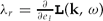 and
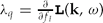 are decreasing.
Combining proposition 3 with strict versions of the last inequalities we get:
Proposition 5. (Dependence between shadow prices individual supply) Suppose the inverse demand curve e I ↦ λr(e I) is strictly decreasing. If eI, ei are ∓ dependent, then λr, e iare ± dependent. Thus, ∓ dependence between eI, ei, confers a ‘β-value’ on ei of opposite sign. In short, ∓ dependence, yields a corresponding ± bonus.
If f I ↦ λq(f I) is strictly decreasing, quite similar statements obtain for λq and fI.
In particular, if standard present-value calculations, based on autarky assumptions, prove project i ‘in the money’, and fI, fi are positively dependent, then it better be fairly ‘deep in the money’. Ex ante ki is valued at the margin by the formula

It enters here, as a separate part, the commonplace covariance format of pricing:

5. Parallel production
For further illustration, consider a simple instance where project i contributes a steady income flow ϕi over the time interval [0, Ti]. Revenues are discounted continuously at rate ρ > 0 so that the said project furnishes present value

Let T i : = r i/ϕi where r i ≥ 0 denotes the amount of resources devoted to project i. Consequently, presuming that capacity adjustment is impossible

where ϕi = Φi(k i, ω) ≥ 0. For simpler notation write ϕI := ∑i∈I ϕi. Also for simplicity, posit πi(k i, ω, q i, r i) = q i. Agent i receives resource endowment ei(ω) at the second stage, this yielding aggregate e I(ω) := ∑i∈Ie i(ω). At that stage, given kS = (k i)i∈S and ω, coalition S ⊆ I could achieve

by pooling its members' objectives, technologies, and endowments. Let λr(ω) ≥ 0 be the Lagrange multiplier associated to ∑i∈Ir i ≤ ∑i∈Ie i(ω). This state-dependent shadow price should satisfy

Simple calculations give a multiplier λr = exp(−ρe I/ϕI), which decreases strictly in eI so that proposition 5 applies:
• If eI, ei are negatively (positively) dependent, then cov(λr, e i) has the opposite sign. Simple calculations also show that
• the aggregate endowment eI is distributed according to production flows; that is, the optimal resource allocation has
 .
 .
Agents with relatively large ϕi will thus take substantial parts of eI. Such linear sharing is known from mutual insurance where ϕi denotes the risk tolerance of agent i (see Borch, Reference Borch1968; Magill and Quinzii, Reference Magill and Quinzii1996; Wilson, Reference Wilson1968; Flåm, Reference Flåm2002). The advantages of pooling not perfectly correlated risks are evident: accidentally ‘starving’ agents are helped by more fortunate fellows. The receivers will reciprocate once providence smiles on them. The resulting ex post payment

gives the second-stage core solution. This payment has two terms: first, the production part

second, the net financial transfer

Since these transfers sum to zero, the second-stage, total value equals  . As we might expect:
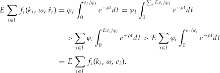
• the total ‘cake’ increases by cooperation

The last inequality holds for all kI and ω. It stems from ∫0Te −ρtdt being strictly concave in T. Therefore, by Jensen's inequality

this attesting to the advantage of pooling resources. Uncertainty is likely to enforce this feature – and especially so when all risks are idiosyncratic. To wit:
• if each individual endowment ei is random, but their sum eI is not, the gains from cooperation are twofold: they stem, first, from substitutions and, second, from smoothing
6. Comparative risk advantage
David Ricardo, considering international trade in several goods, studied comparative advantages (Dixit and Normann, Reference Dixit and Normann1982). This section briefly takes up similar issues. Here, however, merely one good comes into play. Accordingly, we might expect that production best be undertaken by the most efficient agents. Under uncertainty this need not be so. Indeed, rather inefficient producers may warrant premiums as suppliers of stability and insurance. This feature becomes particularly pronounced when the risk of some inefficient party stays out of line with others.
To illustrate, let there be no capacity limit k i = +∞), no capacity adjustments (Δk i = 0), and no endowment (ei = 0). Also, instead of payoff consider cost C i := −πi with

The operator [r]+ := max{0, r} preserves the positive part of the real number r. The parameter di is construed as i's ‘inelastic demand’. If endogenous supply qi falls short of demand di, the residual amount di − qi must be procured from external sources at unit cost κ. Let

where the parameter P i ∈ (0, 1) is prescribed and b i (ω) ∈ {0, 1} is a binomial variable. The latter takes the value 1 with probability p i ∈ [0, 1), leaving then only the proportion Pi of capital ki intact. With complementary probability p i := 1 − p i, all of ki remains productive. Under autarky agent i will minimize expected cost

with respect to ki. In that optic his best choice becomes

Next open up for cooperation; that is, for free trade. That opening will minimize

with respect to (ki). Equivalently, trade minimizes

Indeed, a minimizing (qi) in F(k) satisfies q i ≤ d i for all I, whence ∑i∈I [d i − q i]+ = [∑i∈I(d i − q i)]+ and  (k) ≤ F(k). Conversely, given a minimizing profile
 i) in (k), there exists for each i a q i ≤ d i such that ∑i∈Iq i = ∑i∈Ii. Hence [∑i∈Id i − i]+ = ∑i∈I [d i − q i]+ so that F(k) ≤ (k).
For the sake of transparency, suppose finally that there are only two agents. Objective (8) then takes the reduced form

We assume κ1 < κ2 < κ and briefly discuss three cooperative cases next:
1. Absent uncertainty, when p 1 = p 2 = 0, we get k 1 = d 1 + d 2 and k 2 = 0. Then, to no surprise, the most efficient agent produces all.
2. Only the efficient agent is at risk; that is, p 1 > 0, p 2 = 0, in which case (9) specializes to
Note that when total supply equals d 1 + d 2, the expected marginal production costs are κ1 − κ(p 1P 1 + p 1) for agent 1 and κ2 − κ for agent 2. If the latter is smaller, then, somewhat surprisingly, the cost efficient agent better be inactive, leaving production entirely to his high-cost associate (i.e. k 1 = 0, k 2 = d 1 + d 2). The latter is able to compensate qua insurer for his own handicaps qua producer.
3. Both are risk exposed, but in perfectly opposed manner; that is, p 1 > 0, p 2 = 1 −p 1, and b 1(ω) + b 2 (ω) = 1. Then (9) reads


The structure of the optimal solution is similar to the preceding case, but outside procurement could become more attractive. In particular, if κ1 > κ(p 1P 1 + p 1) and κ2 > κ(p 2P 2 + p 2), it is not worth anyone's while to produce.
Non-smooth objectives like (7), reflecting ‘hit-or-miss’ situations, inspire new measures of risk, notably so-called Conditional Value-at-Risk (Rockafellar and Uryasev, Reference Rockafellar and Uryasev2000).
7. Environmental games and quota trade
As noted, the core imputation (6) reduces essentially to competitive equilibrium in endogenous markets for capital and contingent commodities. We can hardly presume though, that imperfectly informed, human-like players will reach such equilibrium right away. More realistically, they need time to adapt and learn. The classical branch of economics that deals with competitive markets fails, however, to account for adaptation and learning.
Our set-up invites reconsideration of these matters. But first we address a related question, already invoked, namely: how is uncertainty described or formalized? In this regard the necessary prerequisites are often few and reasonable. To illustrate, suppose a discrete-time process ω t, t = 0, 1, . . . of independent random variates, all distributed as the underlying ω, can be simulated or observed step by step. Then the prospects are good for reaching a stable equilibrium over time. Indeed, recent studies explore the convergence of repeated, bilateral exchange towards an efficient steady state (Ermoliev et al., Reference Ermoliev, Klaassen and Nentjes1996; Ermoliev et al., Reference Ermoliev, Michalevich and Nentjes2000a; Ermoliev et al., Reference Ermoliev, Keyzer and Norkin2000b; Flåm and Godal, Reference Flåm and Godal2007).
At this point only the coupling constraint k I := ∑i∈Ik i ≤ ∑i∈Ik i =: k I becomes crucial. Suppose that k I reflects an aggregate upper bound – say, on the catch of valuable fish or the emission of greenhouse gases. Hence k I = k I holds throughout, and payoffs πi(k I, ·) could depend on k I.
An environmental game may thus unfold in which players trade quotas ex ante and contingent commodities ex post. While adjustment of quotas is sluggish, other variables are easily and quickly changed. So, to simplify, suppose that second-stage markets clear ‘instantaneously’, and that Δk i = 0 there. As a by-product this clearing generates Lagrange multipliers λq(ω). It also gives reduced functions πi(k i, ω) := πi(k i, ω,  i,
 i) and f i(k i, ω) := f i(k i, ω, i, i), embodying optimal choices i, i. Let st > 0 – for instance, st = A/(t + B) with A, B > 0 – be a sequence of step sizes that satisfies
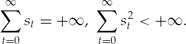
Exchange begins at time t = 0, with s = s 0, ω = ω 0, k i = k i.
• Select a pair of agents i, j ∈ I at random. These hold stocks ki and kj respectively.
• Calculate their realized marginal returns on capital
• Transfer s(mi − mj) to i from j, this giving the two parties new holdings
• Increase time t by 1.
• Update the step size s ← s t, and observe a new independent ω ← ω t.
• Continue to select a pair of agents until convergence.


Convergence obtains as in (Ermoliev et al., Reference Ermoliev, Michalevich and Nentjes2000a; Ermoliev et al., Reference Ermoliev, Keyzer and Norkin2000b; Flåm and Godal, Reference Flåm and Godal2007). Note that trade is voluntary and driven by perceived prospects for mutual improvements. It happens out of equilibrium, uses money as instrument, and requires no revelation of private information. We might reasonably presume that each transaction be Pareto improving for the two interlocutors; see Goldman and Starr (Reference Goldman and Starr1982) and references therein. While still away from equilibrium, the side payments that go along with a bilateral exchange could result from bargaining (Rubinstein and Wolinsky, Reference Rubinstein and Wolinsky1990). Under alternating offers the perfect equilibrium of non-cooperative bargaining depends on personal discount factors – and on who proposes first (Osborne and Rubinstein, Reference Osborne and Rubinstein1994). Note that exchange is conditioned by the prevailing state – and construed as relatively small in size. We hesitate, therefore, in rigging precise data, rules, or protocols on negotiations, and rather leave division of short-term gains unspecified. Accordingly, no monetary payments are mentioned. We simply let the capacity transfer be motivated by the difference mi − mj in marginal payoffs (Kolstad and Guzman, Reference Kolstad and Guzman1999).
8. Concluding remarks
Most often, for practical and realistic analysis, the planning horizon should extend beyond two stages. The reasons are evident: uncertainty is unveiled gradually, over many steps – and there are repeated opportunities to implement recourse actions. Such complexity notwithstanding, if one is willing to work in suitably high dimensions, problem format (1) is rich enough to comprise as many stages and commodities as deemed necessary (see Evstigneev and Flåm, Reference Evstigneev and Flåm2001a,Reference Evstigneev and Flåmb). We may think of all future intervals as compressed into a single second period. Moreover, the short time horizon seems appropriate when agents hesitate in committing to more than time-limited contracts.
While the preceding models were stylized, extensions can easily incorporate greater realism and more detail. Still, rather simple versions already bring out the wide applicability of stochastic production games. They facilitate studies of quasi-markets or market-like settings affected by sequential decisions and much uncertainty. Several theories, and attending practices, then come on stage. Included are finance, insurance, stochastic optimization, and Monte Carlo simulation. Since these disciplines have complementary concerns and perspectives, they supplement each other. Together they facilitate a rich analysis of how players should or would fare. Particularly important is the possibility to deal with absence or incompleteness of markets. In addition, the presence of public bads or goods – or widespread externalities – need not preclude reasonable coordination and relative efficiency. Troublesome though, are economies of scale. In that case Lagrange multipliers may not exist – and core solutions are harder to find, if any (Evstigneev and Flåm, Reference Evstigneev and Flåm2001b).
Especially important are concerns with expendability and reversibility of capacity choice (Abel et al., Reference Abel, Dixit, Eberly and Pindyck1996; Arrow and Fisher, Reference Arrow and Fisher1974; Dixit and Pindyck, Reference Dixit and Pindyck1996, Reference Dixit, Pindyck, Brennan and Trigeorgis2000; Dixit et al., Reference Dixit, Pindyck and Sødal1999; Henry, Reference Henry1974). Worries relate then to adjustment costs that are convex at the origin. Such instances fit, however, well within the frames of stochastic production games. In particular, we may estimate the value of perfect information (Pflug, Reference Pflug, Marti, Ermoliev and Pflug2004).
Appendix
Proof of proposition 1. Recall that any bivariate, real-valued function  satisfies

(This inequality, named weak duality in optimization theory, reflects the last-mover advantage in zero-sum, two-person, non-cooperative games.) In the present context, at the second stage, given k = (ki) and ω, let ξ := (Δk i, r i, q i)i∈S, and associate the contingent Lagrangian

to coalition S. Note that

if ∑i∈Sr i ≤ ∑i∈Se i(ω) & ∑i∈Sq i ≤ ∑i∈Sf i(k i, ω, Δk i, r i); otherwise the minimal value equals −∞. Consequently

When λ = Λ ≥ 0 is a Lagrange multiplier, coalition S will not block the proposed payment scheme because
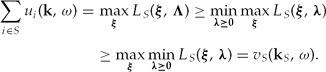
In particular, ∑i∈Iu i(k, ω) ≥ v I(k, ω). Since the converse inequality holds by assumption, Pareto efficiency also obtains. When e I(ω) and ∑i∈If i(k i, ω, 0, e i (ω)) are both positive, the Slater condition holds – hence existence of multipliers is ensured.
Proof of proposition 2. Associate here another Lagrangian 

to coalition S. Note that

if ∑i∈Sr i ≤ ∑i∈Se i(ω) and ∑i∈Sq i ≤ ∑i ∈ Sf i(k i, ω, Δk i, r i) almost surely, and ∑i∈Sk i ≤ ∑i ∈ Sk i. Otherwise the minimal expected value equals −∞. Consequently, still writing ξ = Δk i, r i, q i)i∈S, we get

When Λ, μ are Lagrange multipliers, coalition S will not block the proposed payment scheme (Ui) because

In particular, ∑i∈IU i ≥ v I(k I). Since the converse inequality holds by assumption, Pareto efficiency again obtains. The presumed positivity guarantees that the Slater condition holds whence multipliers are available.


