

1. Introduction
Wave turbulence has a six-decade-long successful record in describing inter-scale energy transfers in nonlinear wave media in geophysics – internal inertia gravity waves (Olbers Reference Olbers1976; Lvov & Tabak Reference Lvov and Tabak2001), surface gravity waves (Hasselmann Reference Hasselmann1962; Zakharov & Filonenko Reference Zakharov and Filonenko1967b) and capillary waves (Zakharov & Filonenko Reference Zakharov and Filonenko1967a), Rossby waves (Zakharov & Piterbarg Reference Zakharov and Piterbarg1988), inertial waves (Galtier Reference Galtier2003), astrophysics – e.g. plasma (Sagdeev & Galeev Reference Sagdeev and Galeev1969; Zakharov et al. Reference Zakharov1972) – solid-state physics (Ziman Reference Ziman2001), acoustic waves (Zakharov & Sagdeev Reference Zakharov and Sagdeev1970), vibrating plates (Düring, Josserand & Rica Reference Düring, Josserand and Rica2006) and Bose–Einstein condensates (Nazarenko Reference Nazarenko2011).
In addition to a close formal similarity to hydrodynamic turbulence, the large theoretical relevance of wave turbulence is related to the derivation of non-equilibrium cascade states known as the Kolmogorov–Zakharov (KZ) solutions (Zakharov, L'vov & Falkovich Reference Zakharov, L'vov and Falkovich1992). Unlike the ‘dimensional’ Kolmogorov spectrum of three-dimensional (3-D) turbulence, the KZ spectra are analytical solutions of the equation that represents the main object of wave turbulence theory, namely the wave kinetic equation (WKE). The WKE describes the time evolution of the spectral energy density due to the nonlinear resonant energy transfers between different wave modes.
Non-zero inter-scale energy fluxes are a fundamental feature of wave turbulence that is still far from being fully understood – see e.g. the recent works Hrabski & Pan (Reference Hrabski and Pan2022) and Dematteis & Lvov (Reference Dematteis and Lvov2021). In geophysical applications, the study of wave turbulence fluxes dates back to the early 1980s for internal waves (McComas & Müller Reference McComas and Müller1981; Holloway, Henyey & Pomphrey Reference Holloway, Henyey and Pomphrey1986) and surface gravity waves (Hasselmann & Hasselmann Reference Hasselmann and Hasselmann1981). Those early studies relied mainly on diffusive approximations of the collision operator, the right-hand side of the WKE that describes the irreversible modal energy transfers due to wave–wave interactions. Subsequent improvements of the approximations to flux computations led to important theoretical and numerical tools that are used up to this day. For the surface gravity wave problem, the numerical schemes currently employed in the WAM global model of wave forecasting (Hasselmann & Hasselmann Reference Hasselmann and Hasselmann1985; Resio & Perrie Reference Resio and Perrie1991; Komen et al. Reference Komen, Cavaleri, Donelan, Hasselmann, Hasselmann and Janssen1996; Janssen Reference Janssen2004) use approximations of the main resonant wave quartets that are responsible for the direct and inverse cascade of energy and wave action through the wave spectrum. This allows for accurate predictions of the global sea states, explaining, for instance, the formation of the large oceanic swells from an inverse cascade process towards the long waves. In the ocean interior, the direct cascade in the oceanic internal wavefield due to resonant wave triads is modelled by what is called the fine-scale parametrization of oceanic mixing and dissipation (Gregg (Reference Gregg1989), Henyey (Reference Henyey1991) and Polzin, Toole & Schmitt (Reference Polzin, Toole and Schmitt1995)). The fine-scale parametrization is a fundamental component of the global models of ocean circulation (Polzin Reference Polzin2009; MacKinnon et al. Reference MacKinnon2017; Whalen et al. Reference Whalen, de Lavergne, Garabato, Klymak, Mackinnon and Sheen2020; Musgrave et al. Reference Musgrave, Pollmann, Kelly and Nikurashin2022). The scaling of this phenomenological parametrization is based on the ‘induced diffusion’ approximation of the WKE of internal waves (McComas & Bretherton Reference McComas and Bretherton1977). In the fine-scale parametrization framework, a downscale flux in the internal waves is associated with the production of mixing and dissipation by the turbulence that is generated when the internal waves overturn and break due to hydrodynamic instabilities. This mixing allows for bottom dense water to slowly upwell towards the surface at low latitudes, with major consequences on the meridional overturning circulation in the ocean (Thorpe Reference Thorpe2005; Garabato & Meredith Reference Garabato and Meredith2022). Both of these notable examples, oceanic surface and internal waves, require understanding of the inter-scale fluxes being transferred through a random bath of resonantly interacting waves. This understanding is important not only for the quantification of the wavefield itself, but also for the paramount implications of the coupling of these systems with the atmosphere and other components of the climate system.
The approximation schemes mentioned above make use of uncontrolled, often empirical approximations. From a theoretical perspective, the computation of energy fluxes from the collision operator of the WKE is elusive, since the collision operator itself is vanishing in a stationary state. For the KZ spectra, as explained in Zakharov et al. (Reference Zakharov, L'vov and Falkovich1992) and in § 3.1 below, there is an indeterminate expression of the type  $0/0$ that requires regularization (using L'Hôpital's rule). The flux is thus given by the coefficient of the next-order term in a Taylor series expansion of the collision operator, centred in the KZ exponent (Zakharov et al. Reference Zakharov, L'vov and Falkovich1992). However, for non-KZ stationary states, which are relevant solutions e.g. in anisotropic systems like Rossby waves (Nazarenko Reference Nazarenko2011) and internal waves (Lvov et al. Reference Lvov, Tabak, Polzin and Yokoyama2010), in general it is not clear how to calculate the flux from the collision operator. Moreover, some of the early quantifications of energy transfers failed to notice the key difference between the energy density time increment and the actual energy flux. The idea can be explained with the help of a one-dimensional (1-D) example. Let
 $\dot e_p$ be the energy density rate of change, and
 $F_p$ the energy flux, where
 $p$ is the scalar wavenumber variable. In general, the energy balance for an infinitesimal interval
 $[p,p+{\rm d}p]$ reads
 $\dot e_p\, {\rm d}p=F_p-F_{p+{\rm d}p}$. A slightly positive
 $\dot e_p$ could correspond to a negative or positive flux alike, as long as
 $F_p$ is a decreasing function of
 $p$. When
 $\dot e_p$ is vanishing instead – which defines stationary conditions – the flux is constant in
 $p$, but its value cannot be determined from
 $\dot e_p$ alone. Thus the sign of
 $\dot e_p$ is quite unrelated to the direction and magnitude of
 $F_p$! This objection was put forward in Holloway (Reference Holloway1980), arguing that close to a stationary state, the small value of
 $\dot e_p$ has nothing to do with the time scale of the energy pathways, or more precisely with the ‘residence time’ of energy in the wavefield. This time scale is dictated by the magnitude of
 $F_p$. Even when the difference between the two quantities has been treated correctly, much more emphasis has been given in the literature to the evaluation of the rate (
 $\dot e_p$ in the intuitive example) rather than to the actual flux (
 $F_p$). Finally, another remarkable theoretical need is the generalization of the theory of the fluxes of conserved quantities to wave systems that are not self-similar, since the bulk of the theory was developed mainly for scale-invariant spectra (Zakharov et al. Reference Zakharov, L'vov and Falkovich1992; Nazarenko Reference Nazarenko2011).
To summarize, the existing body of literature is focused on calculating energy fluxes in stationary isotropic scale-invariant wave turbulence systems. Yet, the kinetic equation contains a lot of information about wave–wave interactions that is not currently utilized. Here, we propose a way to calculate energy fluxes that is free of these limitations.
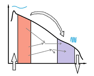
In this work, we focus on the study of three-wave collision operators, and tackle the problem of quantifying the associated energy transfer between two generic disjoint control volumes in Fourier space. We introduce a logical operator, namely the characteristic interaction weight; this weight allows us to extract the flux between the two control volumes from the collision operator, by singling out those triads of wavenumbers that participate in a direct energetic link between the control volumes themselves. The definition of the characteristic interaction weight is based on a fundamental symmetry of the three-wave collision operators, namely the detailed energy conservation property (Kraichnan Reference Kraichnan1959). As a result, any non-vanishing energy fluxes, even in a stationary state, can be calculated by integration of a well-defined non-vanishing function. We call this function the transfer integral of the problem. Note that these calculations are exact: they do not employ any approximation other than the assumption of validity of the wave kinetic equation. Moreover, self-similarity is not required. Our results establish a formal wave turbulence parallel to the Kraichnan (Reference Kraichnan1959) computation of energy fluxes for hydrodynamic turbulence at high Reynolds numbers, versions of which have been used for different models of turbulence (e.g. see Kraichnan Reference Kraichnan1975; Rose & Sulem Reference Rose and Sulem1978; Eyink Reference Eyink1994).
In our approach, we postulate a governing wave kinetic equation with an inertial range of scales. In support of this kinetic assumption, we appeal to the current fervent research towards a rigorous justification of the WKE from the deterministic equations of motion (Choi, Lvov & Nazarenko Reference Choi, Lvov and Nazarenko2004; Nazarenko Reference Nazarenko2011; Lukkarinen & Spohn Reference Lukkarinen and Spohn2011; Eyink & Shi Reference Eyink and Shi2012; Chibbaro, Dematteis & Rondoni Reference Chibbaro, Dematteis and Rondoni2018; Onorato & Dematteis Reference Onorato and Dematteis2020; Buckmaster et al. Reference Buckmaster, Germain, Hani and Shatah2021; Deng & Hani Reference Deng and Hani2021a,Reference Deng and Hanib; Banks et al. Reference Banks, Buckmaster, Korotkevich, Kovačič and Shatah2022; Rosenzweig & Staffilani Reference Rosenzweig and Staffilani2022).
The paper is organized as follows. In the remainder of § 1, we set the stage by introducing the WKE and its relevant properties. Section 2 contains our ‘main statement’ in the form of a formula for the computation of energy transfers between two generic control volumes in spectral space. Its application to isotropic systems is treated in § 3, where the standard flux formula of isotropic wave turbulence is recovered as a particular case of the main statement for adjacent control volumes, and the concept of transfer integral is defined. In § 4, we illustrate the results for the surface capillary wave example, including a detailed quantification of the locality properties of the system. Section 5 is devoted to the application to anisotropic systems, followed by a practical illustration for the internal wave problem in § 6. In § 7, we exploit the transfer-integral formulas derived previously to calculate the convergence conditions for the energy flux and to define a number  $w$ quantifying the level of locality of the energy transfer. We discuss and summarize our results in § 8.
1.1. Wave kinetic equation
We start from the WKE of a system with three-wave resonant interactions (Zakharov et al. Reference Zakharov, L'vov and Falkovich1992; Nazarenko Reference Nazarenko2011):
 \begin{equation} \left. \begin{aligned} & \frac{\partial n_{\boldsymbol{p}}}{\partial t} = \int_{\mathbb{R}^d\times \mathbb{R}^d} {\rm d}\boldsymbol{p}_1 \,{\rm d}\boldsymbol{p}_2\, \mathcal{J}(\boldsymbol{p};\boldsymbol{p}_1,\boldsymbol{p}_2),\quad\mathcal{J}(\boldsymbol{p};\boldsymbol{p}_1,\boldsymbol{p}_2) = \mathcal{R}^0_{12} - \mathcal{R}^1_{02} - \mathcal{R}^2_{01},\\ & \text{where}\quad \mathcal{R}^0_{12} = 4{\rm \pi}\,|V^0_{12}|^2\, f^0_{12}\,\delta(\boldsymbol{p}^0_{12})\,\delta(\omega^0_{12}),\quad f^0_{12} = n_1n_2-n_{\boldsymbol{p}}(n_1+n_2), \end{aligned} \right\} \end{equation}
and  $\boldsymbol {p}^0_{12}=\boldsymbol {p}-\boldsymbol {p}_1-\boldsymbol {p}_2$,
 $\omega ^0_{12}=\omega _{\boldsymbol {p}}-\omega _1-\omega _2$. The variable
 $n_{\boldsymbol {p}}$ is the
 $d$-dimensional wave-action spectral density at wavenumber
 $\boldsymbol {p}\in \mathbb {R}^d$. For simplicity, we denote
 $p_i$ by its index
 $i$ in subscripts and superscripts, and the wavenumber variable
 $\boldsymbol {p}$ by index
 $0$. Action can be viewed as the ‘number’ of waves with a given wavenumber. The function
 $\omega _{\boldsymbol {p}}$ is the linear dispersion relation of the system, taking the positive branch by convention. Consequently, wave action multiplied by frequency
 $\omega _{\boldsymbol {p}} n_{\boldsymbol {p}}$ is the quadratic spectral energy density. Note that wavenumbers are vectors in
 $\mathbb {R}^d$, while frequencies are always positive scalars. The factor
 $V^0_{12}$ is the interaction matrix element (or scattering cross-section) describing the transfer of wave action among the members of a triad composed of three wavenumbers
 $\boldsymbol {p},\boldsymbol {p}_1,\boldsymbol {p}_2$.
 $V^0_{12}$ is invariant under permutation of the lower indices
 $1$ and
 $2$, and therefore so is
 $\mathcal {R}^0_{12}$. We refer to
 $\mathcal {J}(\boldsymbol {p};\boldsymbol {p}_1,\boldsymbol {p}_2)$ as the interaction kernel (or collision integrand) associated with the given WKE. The right-hand side of (1.1) is then called the collision integral, a quadratic functional in the action density
 $n_{\boldsymbol {p}}$. The collision integral captures the irreversible transfers of action between different modes as the outcome of nonlinear interactions between triads of wavenumbers in resonance with each other.
1.2. Resonant manifold
Let the dispersion relation of the system be of the form  $\omega _{\boldsymbol {p}} = \omega (|p_1|,\ldots,|p_d|)$, positive-definite, monotonic in each component, and such that it allows for non-trivial solution of the three resonant conditions
 \begin{align} {\rm(I)}: \left\{\begin{array}{ll} \boldsymbol{p} = \boldsymbol{p}_1+\boldsymbol{p}_2,\\ \omega_{\boldsymbol{p}}=\omega_1+\omega_2, \end{array}\right. \quad {\rm(II)}:\left\{\begin{array}{ll} \boldsymbol{p}_1 = \boldsymbol{p}+\boldsymbol{p}_2,\\ \omega_1=\omega_{\boldsymbol{p}}+\omega_2, \end{array}\right.\quad {\rm(III)}:\left\{\begin{array}{ll} \boldsymbol{p}_2 = \boldsymbol{p}+\boldsymbol{p}_1,\\ \omega_2=\omega_{\boldsymbol{p}}+\omega_1.\end{array}\right. \end{align}
For instance, limited to power-law dispersion relations  $\omega (\boldsymbol {p})\propto |\boldsymbol {p}|^\alpha$, the condition
 $\alpha >1$ is necessary and sufficient for the existence of solutions to (1.2a–c) (Zakharov et al. Reference Zakharov, L'vov and Falkovich1992).
Note that the invariance upon permutation of the indices  $1,2$ in
 $|V^0_{12}|$ and
 $f^0_{12}$ allows us to express the interaction kernel as
 $\mathcal {J}(\boldsymbol {p};\boldsymbol {p}_1,\boldsymbol {p}_2) = \mathcal {R}^0_{12} - 2\mathcal {R}^1_{02}$. This, in turn, allows us in a completely general way to have to deal with only resonance types I (i.e. the sum interactions) and II (i.e. the difference interactions). To simplify the notation in the following, let us denote by
 $\mathcal {J}^{(l)}(\boldsymbol {p},\boldsymbol {p}_1,\boldsymbol {p}_2)$, with
 $l=\textrm {I},\textrm {II},\textrm {III}$, the three terms
 $\mathcal {R}^0_{12} ,-\mathcal {R}^1_{02},-\mathcal {R}^2_{01}$, respectively.
In general, the WKE can then be reduced to
 \begin{equation} \frac{\partial n_{\boldsymbol{p}}}{\partial t} = \sum_l \int_{\varOmega_l} {\rm d}\varOmega_l\,J^{(l)}, \quad\text{with } l={\rm I},{\rm II},{\rm III}, \end{equation}
where  $J^{(l)}$ is the result of analytical integration of the
 $d+1$ independent delta functions, and
 $\varOmega _l$ is a
 $(d-1)$-dimensional representation of the respective branch of the resonant manifold. Note that each of the resonant conditions in (1.2a–c) can have multiple independent solutions (cf. § 6), in which case in (1.3), a summation over the independent solutions of each branch is implied. Once the WKE collision integral is suitably expressed in the form (1.3), integration over the remaining
 $d-1$ degrees of freedom can be performed. The integration can be performed either analytically or numerically depending on the particular situation.
1.3. Detailed energy conservation
We end this introductory section by highlighting a fundamental property of the interaction kernel. The three-wave resonant interactions in the collision integral (1.1) satisfy detailed energy conservation (Onsager Reference Onsager1949; Kraichnan Reference Kraichnan1959; Hasselmann Reference Hasselmann1966; Rose & Sulem Reference Rose and Sulem1978; Eyink Reference Eyink1994).
Property: detailed energy conservation. We define the quantity
 \begin{equation} {\mathcal{Z}}(\boldsymbol{p}_{a},\boldsymbol{p}_b,\boldsymbol{p}_c)= \omega_a\,\mathcal{J}(\boldsymbol{p}_{a};\boldsymbol{p}_b,\boldsymbol{p}_c) + \omega_b\,\mathcal{J}(\boldsymbol{p}_{b};\boldsymbol{p}_a,\boldsymbol{p}_c) + \omega_c\,\mathcal{J}(\boldsymbol{p}_{c};\boldsymbol{p}_a,\boldsymbol{p}_b). \end{equation}
Then for any given triad of wavenumbers  $\boldsymbol {p}_a, \boldsymbol {p}_b, \boldsymbol {p}_c$, we have
 \begin{equation} {\mathcal{Z}}(\boldsymbol{p}_{a},\boldsymbol{p}_b,\boldsymbol{p}_c)=0. \end{equation}
A proof is provided in Appendix A. We note that the equality holds in the sense of distributions, since  ${\mathcal {Z}}(\boldsymbol {p}_{a},\boldsymbol {p}_b,\boldsymbol {p}_c)$ contains delta functions.
The physical meaning of  ${\mathcal {Z}}(\boldsymbol {p}_{a},\boldsymbol {p}_b,\boldsymbol {p}_c)$ is the amount of energy generated during the triadic interactions of three wavenumbers. This quantity is zero due to energy conservation, as ensured by the frequency delta functions. We note that this property holds for triads of wavenumbers on the resonant manifold (1.2a–c), as well as for triads of wavenumbers off the resonant manifold.
2. Energy transfer between two disjoint sets of wavenumbers
Equation (1.1) is derived under the assumption that the quadratic energy is a good approximation of the total energy of the system. The quadratic energy density  $\omega _{\boldsymbol {p}} n_{\boldsymbol {p}}$ is preserved exactly by the time evolution of (1.1), representing what is sometimes referred to as an adiabatic invariant (see e.g. § 8.5.1 in Nazarenko Reference Nazarenko2011). Mathematically, this property is enforced by the frequency delta function in the collision integral, which can be interpreted as the condition of energy conservation in the individual triadic interactions. This is captured by the property of detailed energy conservation (1.5).
From now on, we will refer to  $e_{\boldsymbol {p}}=\omega _{\boldsymbol {p}} n_{\boldsymbol {p}}$ simply as the spectral energy density. After multiplying (1.1) by
 $\omega _{\boldsymbol {p}}$, the right-hand side contains the energy transfers between wavenumber
 $\boldsymbol {p}$ and all possible pairs of wavenumbers
 $\boldsymbol {p}_1$ and
 $\boldsymbol {p}_2$ that interact resonantly with
 $\boldsymbol {p}$.
Let us consider  $A\subset \mathbb {R}^d$ and
 $B\subset \mathbb {R}^d$, with
 $A\cap B=\emptyset$, i.e. two disjoint closed subsets of the
 $d$-dimensional Fourier space. For a given specification of the action spectrum
 $n_{\boldsymbol {p}}$, we wish to quantify how much power (energy per unit of time) is transferred instantaneously from set
 $A$ to set
 $B$. The following statement holds.
Main statement: the net power transferred instantaneously from set  $A$ to set
 $B$ under the governing resonant dynamics of (1.1) is given by
 \begin{equation} \mathcal{P}_{A\rightarrow B} ={-}\int_A {\rm d}\,\boldsymbol{p} \omega_{\boldsymbol{p}} \int_{\mathbb{R}^d\times \mathbb{R}^d} {\rm d}\boldsymbol{p}_1 \,{\rm d}\boldsymbol{p}_2 \sum_l\chi_{B}^{(l)}(\boldsymbol{p}_1,\boldsymbol{p}_2)\,\mathcal{J}^{(l)}(\boldsymbol{p},\boldsymbol{p}_1,\boldsymbol{p}_2), \end{equation}
with  $l=\textrm {I},\textrm {II},\textrm {III}$, where
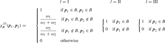
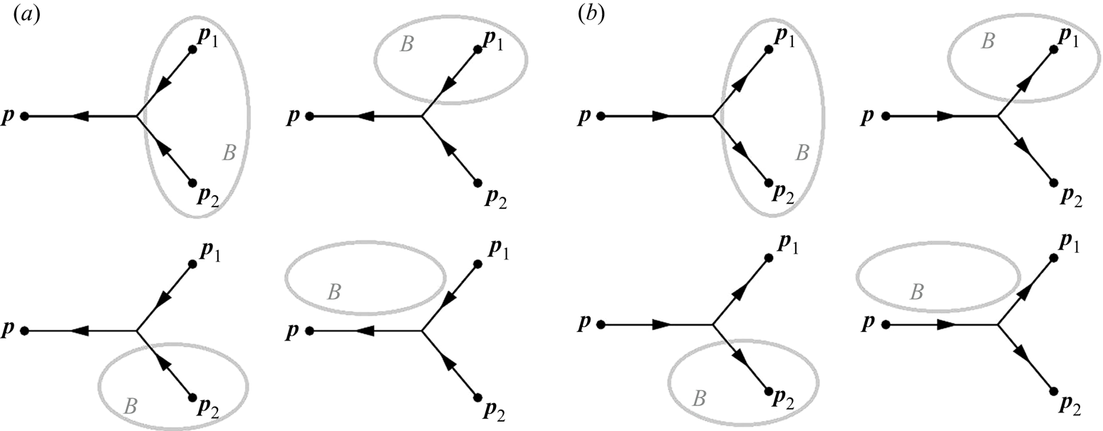
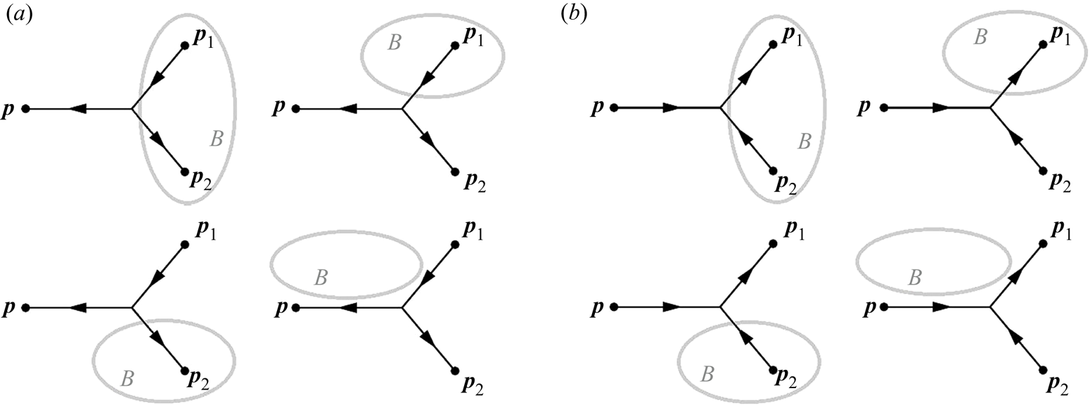
 $\chi _{B}^{(l)}(\boldsymbol {p}_1,\boldsymbol {p}_2)$ is a characteristic interaction weight defined in table 1.
Specification of the interaction weights in (2.1).

We give a sketch of the proof.
The structure of the collision integral can be interpreted as follows. Given any two wavenumbers  $\boldsymbol {p}_1$ and
 $\boldsymbol {p}_2$ in resonance of type
 $l$ with
 $\boldsymbol {p}$, the interaction kernel
 $\mathcal {J}^{(l)}(\boldsymbol {p},\boldsymbol {p}_1,\boldsymbol {p}_2)$ quantifies how much wave-action density (per unit time) is being transferred instantaneously to
 $\boldsymbol {p}$ by the three-wave interaction between the wavenumbers
 $\boldsymbol {p}$,
 $\boldsymbol {p}_1$ and
 $\boldsymbol {p}_2$. When the term is positive, contributing to an increment of
 $n_{\boldsymbol {p}}$, wavenumber
 $\boldsymbol {p}$ is generated as an output of the interaction. When the term is negative, contributing to a decrement of
 $n_{\boldsymbol {p}}$, wavenumber
 $\boldsymbol {p}$ is absorbed as an input of the interaction. The type of three-wave interaction (coded by
 $l$) and the sign of the contribution are enough information to ‘build’ the directed energy diagram associated with the triad. Then integrating over all possible combinations of
 $\boldsymbol {p}_1$ and
 $\boldsymbol {p}_2$ provides the net action increment per unit time for mode
 $\boldsymbol {p}$, i.e. the left-hand side
 $\dot n_{\boldsymbol {p}}$. Multiplying the contribution by
 $\omega _{\boldsymbol {p}}$ allows us to quantify the net energy increment per unit time for mode
 $\boldsymbol {p}$.
Thus a triad of wavenumbers  $\boldsymbol {p},\boldsymbol {p}_1,\boldsymbol {p}_2$ on the resonant manifold leads to an instantaneous change of
 $n_{\boldsymbol {p}}$ to
 $n_{\boldsymbol {p}}+\dot n_{\boldsymbol {p}}|_{012}\,\textrm {d}t$, where we define
 $\dot n_{\boldsymbol {p}}|_{012}:=\mathcal {J}(\boldsymbol {p};\boldsymbol {p}_1,\boldsymbol {p}_2)$ (index
 $0$ is used here to denote wavenumber
 $\boldsymbol {p}$). This increases the energy at
 $\boldsymbol {p}$ by a quantity
 $\dot e_{\boldsymbol {p}}|_{012}\,\textrm {d}t=\omega _{\boldsymbol {p}} \dot n_{\boldsymbol {p}}|_{012}\,\textrm {d}t$. The property of detailed energy conservation (1.5) can now be written equivalently as either of
 \begin{equation} \left. \begin{aligned} \omega_{\boldsymbol{p}}\dot n_{\boldsymbol{p}}|_{012} + \omega_1\dot n_1|_{012} + \omega_2\dot n_2|_{012} & = 0, \\ \dot e_{\boldsymbol{p}}|_{012} + \dot e_1|_{012} + \dot e_2|_{012} & = 0. \end{aligned} \right\} \end{equation}
The reasoning behind the result (2.1) is the following. First, we express  $\dot e_1|_{012}$ and
 $\dot e_2|_{012}$ as a function of
 $\dot e_0|_{012}$, quantifying how much of the energy transferred to wavenumber
 $\boldsymbol {p}$ comes from
 $\boldsymbol {p}_1$, and how much from
 $\boldsymbol {p}_2$. Second, we must consider all possible cases of whether
 $\boldsymbol {p}_1$ and
 $\boldsymbol {p}_2$ are or are not in set
 $B$ to quantify the energy transferred from set
 $B$ to a generic point
 $\boldsymbol {p}\in A$. The interaction weights
 $\chi _{B}^{(l)}(\boldsymbol {p}_1,\boldsymbol {p}_2)$ appear naturally as a result of this calculation. Third, an outer integration over all points
 $\boldsymbol {p}\in A$ yields the total energy transferred from set
 $B$ to set
 $A$ per unit time, i.e. an instantaneous power. The key to the proof, found in Appendix A, is the detailed energy conservation property (1.5).
3. Isotropic systems
3.1. Overview on the theory of energy fluxes
We start here by revisiting the classical arguments for the spectral energy fluxes in wave turbulence. These arguments appear in Zakharov et al. (Reference Zakharov, L'vov and Falkovich1992). Here, we revisit these arguments to prepare for additional insights into spectral energy transfers that are obtained by using our formalism. Our first application of (2.1) is to isotropic scale-invariant systems. We assume a power-law dispersion relation allowing for three-wave resonant interactions and scale-invariant matrix elements with homogeneity exponent  $m$,
 \begin{equation} \omega_p = \kappa p^\alpha,\ \alpha>1,\quad \left|V_{12}^0\right|^2=V_0^2 p^{2m}\, f\left(\frac{p_1}{p},\frac{p_2}{p}\right), \end{equation}
allowing us to look for general solutions to (1.1) of the form
 \begin{equation} n_p=A p^{{-}s}. \end{equation}
Let us start by reviewing some classical results for the energy fluxes in such systems, summarized in Chapter 3 of Zakharov et al. (Reference Zakharov, L'vov and Falkovich1992). In direct analogy with the local energy cascades in isotropic turbulence, it is assumed that the interactions are sufficiently local in Fourier space (Kolmogorov Reference Kolmogorov1941; Kraichnan Reference Kraichnan1959; Rose & Sulem Reference Rose and Sulem1978; Eyink Reference Eyink2005) so that one can assume a differential continuity equation for the 1-D spectral energy density
 \begin{equation} \frac{\partial e_p}{\partial t} = {\rm \pi}(2p)^{(d-1)}\omega_p I_p ={-}\frac{\partial F}{\partial p}, \end{equation}
where the right-hand side of the WKE is interpreted as minus the divergence of a flux  $F$. Here,
 $I_p$ is the collision integral, multiplied by the area of the
 $d$-dimensional sphere. Supposing that there are no energy sources or sinks in an inertial range
 $[\epsilon, M]$, taking
 $\epsilon \to 0$ and
 $M\to \infty$, and solving for the flux
 $F$, one obtains
 \begin{equation} F(p) ={-}{\rm \pi}\int_0^p{\rm d}p'\, (2p')^{(d-1)} \omega_p' I_{p'} . \end{equation}
Interpreting the collision integral as the divergence of a pointwise flux subtends the intuition that energy transfers happen locally in Fourier space. The underlying reasoning involves the following steps. Assume a partition of Fourier space into small boxes of width  $\Delta p$. Assume that the time variation of the energy contained in the box between
 $p$ and
 $p+\Delta p$, say
 $\dot e_{[p,p+\Delta p]}$ is due only to the energy exchanges with its two adjacent boxes. Call
 $F_p$ the net power exchanged at
 $p$, and
 $F_{p+\Delta p}$ the net power exchanged at
 $p+\Delta p$. Express energy conservation for the box under consideration as
 $\dot e_{[p,p+\Delta p]} = F_p - F_{p+\Delta p}.$ Now take
 $\Delta _p\to 0$, and obtain (3.3) by standard transition to a continuum representation. In turbulence, the conditions on how fast the correlations have to decay for the transfers to be sufficiently local are studied in Kraichnan (Reference Kraichnan1959) and Eyink (Reference Eyink1994). In wave turbulence, a transposition of the same arguments leads to the statement that if the collision integral is convergent, then the interactions are sufficiently local for the differential conservation picture (3.3) to hold. For this reason, the convergence conditions for the collision integral in (1.1) are named the ‘locality conditions’ (Zakharov et al. Reference Zakharov, L'vov and Falkovich1992). However, we are also not aware of a rigorous proof of this fact.
When locality holds, the expression for the instantaneous energy flux (3.4) is valid in general, in both stationary and non-stationary conditions. The wave turbulence theory of scale-invariant spectra (Zakharov et al. Reference Zakharov, L'vov and Falkovich1992) focuses on the stationary solutions to (1.1). These can be equilibrium ( $F=0$) or non-equilibrium (
 $F={\rm const}.$) solutions, i.e. the Rayleigh–Jeans (RJ) and the Kolmogorov–Zakharov (KZ) solutions, respectively. The KZ spectrum can be obtained dimensionally or via the Zakharov–Kraichnan conformal transformations (Zakharov & Filonenko Reference Zakharov and Filonenko1967a; Zakharov et al. Reference Zakharov1972), and we have
 \begin{equation} n_p^{RJ} =A p^{-\alpha},\quad n_p^{KZ}=A p^{{-}s_0},\quad \text{with}\ s_0=m+d. \end{equation}
A paradox (only apparent) has to be solved: a constant flux  $F\neq 0$ must result from integrating a vanishing integrand in (3.4)! It is convenient to switch to
 $\omega$ space using the dispersion relation as the change of variables, by defining
 \begin{equation} I_\omega={\rm \pi} (2p)^{d-1} \left(\frac{{\rm d}\omega}{{\rm d}p}\right)^{{-}1}I_p,\quad \text{so that }\ I_\omega = \omega^{\sigma-2}(V_0A)^2\,\mathcal{I}(s), \end{equation}
where  $\mathcal {I}(s)$ is a non-dimensional integral that vanishes in the stationary states, and
 $\sigma = 2(m+d-s)/\alpha$. Now (3.4) reads
 \begin{equation} F(\omega) ={-} \int_0^\omega {\rm d}\omega'\, \omega' I_{\omega'} ={-}\omega^\sigma (V_0A)^2\, \frac{\mathcal{I}(s)}{\sigma}. \end{equation}
At the KZ solution (3.5), we have  $\sigma =0$, and therefore an indeterminate form
 $0/0$. This indeterminate form is then regularized by Taylor-expanding
 $\mathcal {I}(s)$ to first order, or equivalently by using l'Hôpital's rule. We thus obtain
 \begin{equation} F ={-} (V_0A)^2 \left.\frac{{\rm d}\mathcal{I}}{{\rm d}s}\right|_{s=s_0}, \end{equation}
where the locality conditions ensure that  ${\textrm {d}\mathcal {I}}/{\textrm {d}s}|_{s=s_0}$ is finite, with the property that the flux is positive if
 $s_0>\alpha$, i.e. the KZ spectrum is steeper than the equilibrium spectrum. The solution does not exist if
 $s_0<\alpha$. Moreover, note that
 $F$ is independent of
 $\omega$, consistently with stationarity and corresponding to a constant downscale energy flux in the wave turbulence inertial range.
3.2. Application of the main statement (2.1) to isotropic systems
Using integration variables in  $\omega$ space, in isotropic conditions (1.1) simplifies to
 \begin{equation} \left. \begin{aligned} & \frac{\partial n_p}{\partial t} = \frac{v_p}{p^{d-1}}\int_{0}^\infty {\rm d}\omega_1 \left( J^{({\rm I})}(\omega_p;\omega_1,\omega_p-\omega_1)+2 J^{({\rm II})}(\omega_p;\omega_1,\omega_1-\omega_p)\right) ,\\ & \text{where}\quad J^{({\rm I})}(\omega_p;\omega_1,\omega_2) = R^0_{12},\quad J^{({\rm II})}(\omega_p;\omega_1,\omega_2) ={-} R^1_{02},\\ & \text{and}\quad\quad R^0_{12} = 4{\rm \pi} \kappa^{3(1-d)/\alpha} \frac{(\omega\omega_1\omega_2)^{({d-1})/{\alpha}}}{v_p v_1v_2}\,\frac{|V^0_{12}|^2\, f^0_{12}}{\Delta_d}. \end{aligned} \right\} \end{equation}
We have used the notation  $v_p = \partial \omega /\partial p$, and
 $\Delta _d$ is defined by angle integration of the wavenumber delta function given space isotropy, with the dimensions of a wavenumber to the
 $d$th power. We assume a scale-invariant solution
 \begin{equation} n_p = A \omega_p^{{-}x}. \end{equation}
Using these variables, saying that the interaction kernel  $J(\omega _p;\omega _1,\omega _2)$ has homogeneity exponent
 $\gamma _0-2x$, the KZ solution has exponent
 $x=(\gamma _0+3)/2$, and the RJ solution has exponent
 $x=1$.
By formula (2.1), given  $A$ and
 $B$ as two disjoint closed subsets of Fourier space (spanned by
 $\omega \in \mathbb {R}^+$), the instantaneous power delivered from
 $A$ to
 $B$ amounts to
 $$\begin{gather} \mathcal{P}_{A\rightarrow B} ={-}2^{d-1}{\rm \pi} \int_A {\rm d}\omega' \,\omega' \int_0^\infty {\rm d}\omega_1 \left(\chi_{B}^{({\rm I})}(\omega_1)\,J^{({\rm I})}(\omega';\omega_1,\omega'-\omega_1)\right.\nonumber\\ \left.{}+2 \chi_{B}^{({\rm II})}(\omega_1)\, J^{({\rm II})}(\omega';\omega_1,\omega_1-\omega')\right), \end{gather}$$
where the dependence on  $\omega _2$ in the interaction weight is constrained implicitly by
 $\omega _2=\omega '-\omega _1$ in the first line and by
 $\omega _2=\omega _1-\omega '$ in the second line. Let us choose
 $A=[0,\omega ]$,
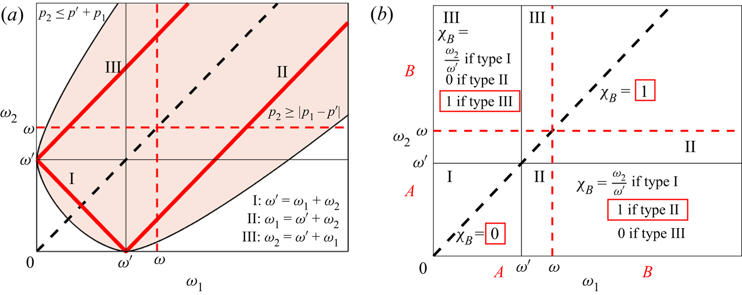
 $B=[\omega,+\infty ]$ to make a concrete calculation in a specific case, noting that in principle this corresponds to the computation in (3.7). As represented in figure 1(b), this choice of sets leads to the major simplification
 \begin{equation} \chi_{B}(\omega_1) = \varTheta(\omega_1-\omega), \end{equation}
where  $\varTheta ({\cdot })$ denotes the Heaviside step function. Moreover, as also shown in figure 1(a), the resonant manifold is such that
 $J^{(\textrm {I})}(\omega ;\omega _1,\omega _1-\omega ')=0$ for
 $\omega _1>\omega '$, and
 $J^{(\textrm {II})}(\omega _p;\omega _1,|\omega '-\omega _1|)=0$ for
 $\omega _1<\omega '$. Thus from (3.11) we obtain
 \begin{equation} \mathcal{P}_{[0,\omega]\rightarrow [\omega,+\infty)} ={-}2^{d}{\rm \pi} \int_0^\omega {\rm d}\omega' \,\omega' \int_\omega^{+\infty} {\rm d}\omega_1\,J^{({\rm II})}(\omega';\omega_1,\omega_1-\omega'). \end{equation}
We are going to derive (3.7) analytically from (3.13), showing that the main statement (2.1) in § 2 encompasses the standard theory of energy fluxes as a particular case. This proof relies on the detailed conservation property (1.5), from which we see that
 \begin{equation} \omega_a\,J(\omega_a;\omega_b,\omega_c) + \omega_b\,J(\omega_b;\omega_a,\omega_c) + \omega_c\, J(\omega_c;\omega_a,\omega_b) =0 \end{equation}
for any triad of wavenumbers  $\boldsymbol {p}, \boldsymbol {p}_1, \boldsymbol {p}_2$. An independent proof by construction for the isotropic case is given in Appendix B. We suggest that the reader examines this proof for an intuitive graphical interpretation of detailed conservation that relies on the symmetries of the resonant manifold.
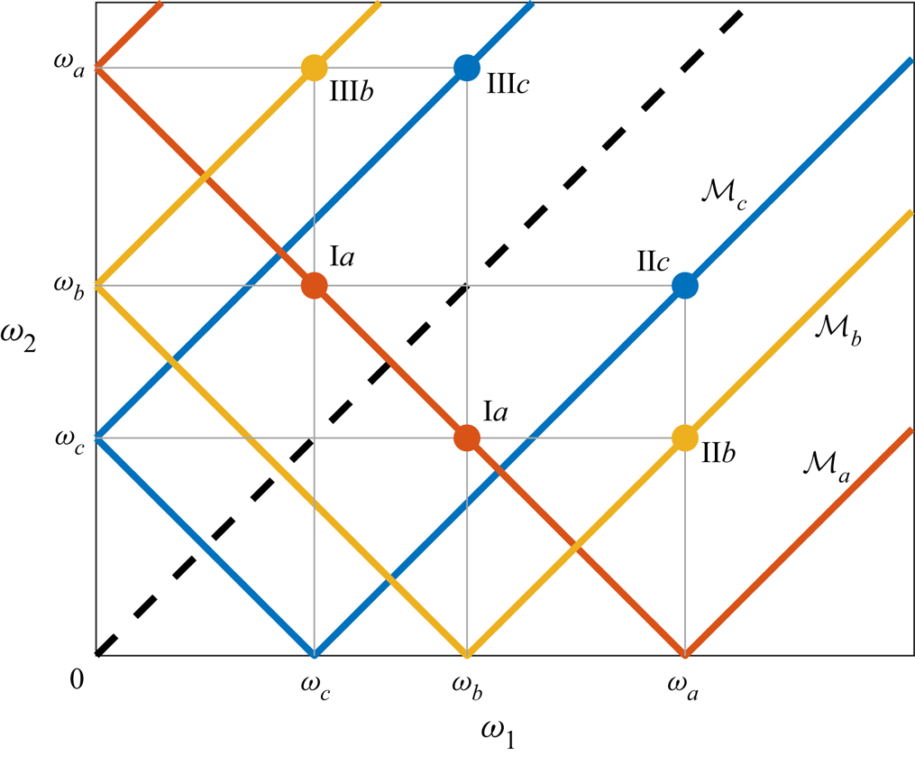
(a) Representation of the resonant manifold in the  $\omega _1\unicode{x2013} \omega _2$ space for triads involving wavenumbers
 $\omega '$,
 $\omega _1$,
 $\omega _2$. Here,
 $\omega$ demarcates the separation between sets
 $A$ and
 $B$ (dashed red lines). The three resonant branches are represented as the three solid red lines labelled I, II, III. The shaded area denotes the region satisfying the wavenumber delta function condition, for a value
 $\alpha >1$. (If
 $\alpha <1$, then this area becomes disjoint from the frequency condition lines, and there are no resonances.) (b) The values of the characteristic interaction weight
 $\chi _{B\rightarrow \omega '}$ in the different regions, as given by the main statement (2.1). Highlighted by a red rectangle are the relevant cases for each region, due to the interaction type present in that region. Exploiting the symmetry with respect to the main diagonal and considering only
 $\omega _2\le \omega _1$ (below the dashed black line), it is clear that
 $\chi _{B\rightarrow \omega '}=\varTheta (\omega _1-\omega )$.

3.3. Proof of the standard flux formula (3.7)
Property: vanishing self-interactions. The following property holds:
 \begin{equation} \int_0^\omega {\rm d}\omega'\int_0^\omega {\rm d}\omega_1 \, J(\omega',\omega_1, |\omega'-\omega_1|)=0, \end{equation}
This follows directly from detailed conservation, as shown in Appendix A.
The meaning of this property is that the integral (3.15) quantifies the flux from  $[0,\omega ]$ to
 $[0,\omega ]$, i.e. self-interactions that amount to no net transfer of energy. This leads to the following important corollary of the main statement (2.1).
Property: Retrieving the standard flux formula for isotropic systems. The standard flux formula (3.7) that is used to calculate the energy flux in isotropic wave turbulence is a direct consequence of (2.1) (main statement) and (3.15).
Proof. Equation (3.13) is derived directly from (2.1), in the particular case of isotropic systems and adjacent control intervals  $A=[0,\omega ]$,
 $B=[\omega,+\infty ]$. Exercising the freedom to add zero (i.e. (3.15)) to (3.13), we obtain
 \begin{align} \mathcal{P}_{[0,\omega]\rightarrow [\omega,+\infty)} &={-}2^{d-1}{\rm \pi} \int_0^\omega {\rm d}\omega'\, \omega'\left[\int_\omega^{+\infty} {\rm d}\omega_1\,J(\omega',\omega_1, |\omega'-\omega_1|) \right.\nonumber\\ & \quad \left. {}+ \int_0^\omega {\rm d}\omega_1\,J(\omega',\omega_1, |\omega'-\omega_1|) \right]\nonumber\\ & ={-}2^{d-1}{\rm \pi} \int_0^\omega {\rm d}\omega'\,\omega'\int_0^{+\infty} {\rm d}\omega_1\, J(\omega',\omega_1, |\omega'-\omega_1|)\nonumber\\ & = \int_0^\omega {\rm d}\omega' \, \omega' I_{\omega'} = F(\omega), \end{align}
which concludes the proof of validity of the usual flux formula (3.7) starting from the main statement (2.1).
As highlighted in (3.16), note that the classical flux expression  $F(\omega )$ (3.7) contains a self-interaction contribution in the interval
 $[0,\omega ]$. This contribution is vanishing due to (3.15). Moreover, (3.7) requires regularization at the KZ solution (see (3.8)). Equation (3.13) is free of such limitations. We elaborate on these points in § 4 by considering surface capillary waves.
3.4. Quantifying locality: the transfer integral
In order to explore the full potential of the main statement (2.1), let us introduce a slight generalization of (3.13). Performing the outer integration up to a smaller frequency  $\tilde \omega <\omega$ allows us to express the power that from the interval
 $[0,\tilde \omega ]$ is delivered instantaneously to
 $[\omega, +\infty )$:
 \begin{equation} \mathcal{P}_{[0,\tilde\omega]\rightarrow [\omega,+\infty)} ={-}2^{d}{\rm \pi} \int_0^{\tilde\omega} {\rm d}\omega' \,\omega' \int_\omega^{+\infty} {\rm d}\omega_1\, J^{({\rm II})}(\omega';\omega_1,\omega_1-\omega'). \end{equation}
This is the wave turbulence analogue of (6.4) in Kraichnan (Reference Kraichnan1959). Recalling that the collision kernel has homogeneity exponent  $\gamma _0-2x$, with a change of variables
 $\varOmega =\omega '/\omega$, we obtain
 \begin{equation} \mathcal{P}_{[0,\tilde\omega]\rightarrow [\omega,+\infty)} = (V_0A)^2 \,\omega^{y+1} \int_{0}^{\tilde\omega/\omega} {\rm d}\varOmega \,T(\varOmega), \end{equation}
where  $y=\gamma _0+2-2x$, with the following.
Definition: transfer integral.
 \begin{equation} T(\varOmega):={-}2^{d}{\rm \pi} (V_0A)^{{-}2}\;\varOmega^{y} \int_{\varOmega^{{-}1}}^{+\infty} {\rm d}\xi \, J^{({\rm II})}(1;\xi,\xi-1) \end{equation}
is the transfer integral of the problem.
The transfer integral is a non-dimensional function that captures the inter-scale ‘structure’ of the energy transfers between two disconnected regions of Fourier space. In particular, it quantifies the direct transfer by a given frequency (smaller than  $\omega$) to all frequencies larger than
 $\omega$. The integral of
 $T(\varOmega )$ up to
 $\tilde \omega /\omega$ gives the distant-transport power exchanged between the two regions
 $[0,\tilde \omega ]$ and
 $[\omega,+\infty )$. Because of the scale invariance of the problem,
 $T(\varOmega )$ is defined uniquely no matter the chosen values of
 $\tilde \omega$ and
 $\omega$. It has to be computed only once, and then the boundaries of the two sets enter the problem as the upper integration boundary and as the scaling factor in (3.18).
Using the power  $\mathcal {P}$ between adjacent sets, by using (3.10)–(3.18), we are able to express the Kolmogorov constant of the problem (Zakharov et al. Reference Zakharov, L'vov and Falkovich1992) as a function of the transfer integral itself, for the KZ solution:
 \begin{equation} n_p^{KZ} = \kappa_K \sqrt{\mathcal{P}} \omega^{{-}x_{KZ}},\quad \kappa_K = \left(V_0 \int_0^1T(\varOmega)\,{\rm d}\varOmega \right)^{{-}1}. \end{equation}
This inter-scale decomposition of the Kolmogorov constant is one of the important implications of the main statement (2.1).
How fast  $\mathcal {P}_{[0,\tilde \omega ]\rightarrow [\omega,+\infty )}$ tends to zero as
 $\tilde \omega /\omega \to 0$ describes how ‘local’ or ‘diffuse’ the energy cascade is (Kraichnan Reference Kraichnan1959). This scaling is going to be dictated by the asymptotics of
 $T(\varOmega )$, and allows us to improve the binary notion of locality (i.e. local/non-local) towards a more quantitative description. How wide should the separation between forcing and dissipation regions be in order to have an inertial range sufficiently disconnected from direct interaction with the boundaries? The transfer integral
 $T(\varOmega )$ provides a key perspective to tackle this type of question, as will be illustrated in the following sections.
4. Isotropic illustration: surface capillary waves
4.1. Application of the main statement (2.1): transfer integral and the Kolmogorov constant
Let us consider the problem of surface capillary waves in isotropic conditions (Pushkarev & Zakharov Reference Pushkarev and Zakharov2000), for which  $d=2$. This system has a dispersion relation with
 $\alpha =\tfrac 32$, allowing for three-wave resonances. After writing the equation in frequency variables and averaging over the angles in
 $\boldsymbol {p}$ space as in (3.9), the interaction kernel has homogeneity exponent
 $\gamma _0-2x$, with
 $\gamma _0=\tfrac 83$. Therefore, the stationary states of the system, in the form
 $n_{\boldsymbol {p}}=A\omega ^{-x}$, are the RJ equilibrium spectrum with
 $x=1$, and the KZ spectrum with
 $x=(\gamma _0+3)/2=\tfrac {17}{6}$. The convergence conditions of the collision integral determine the locality interval
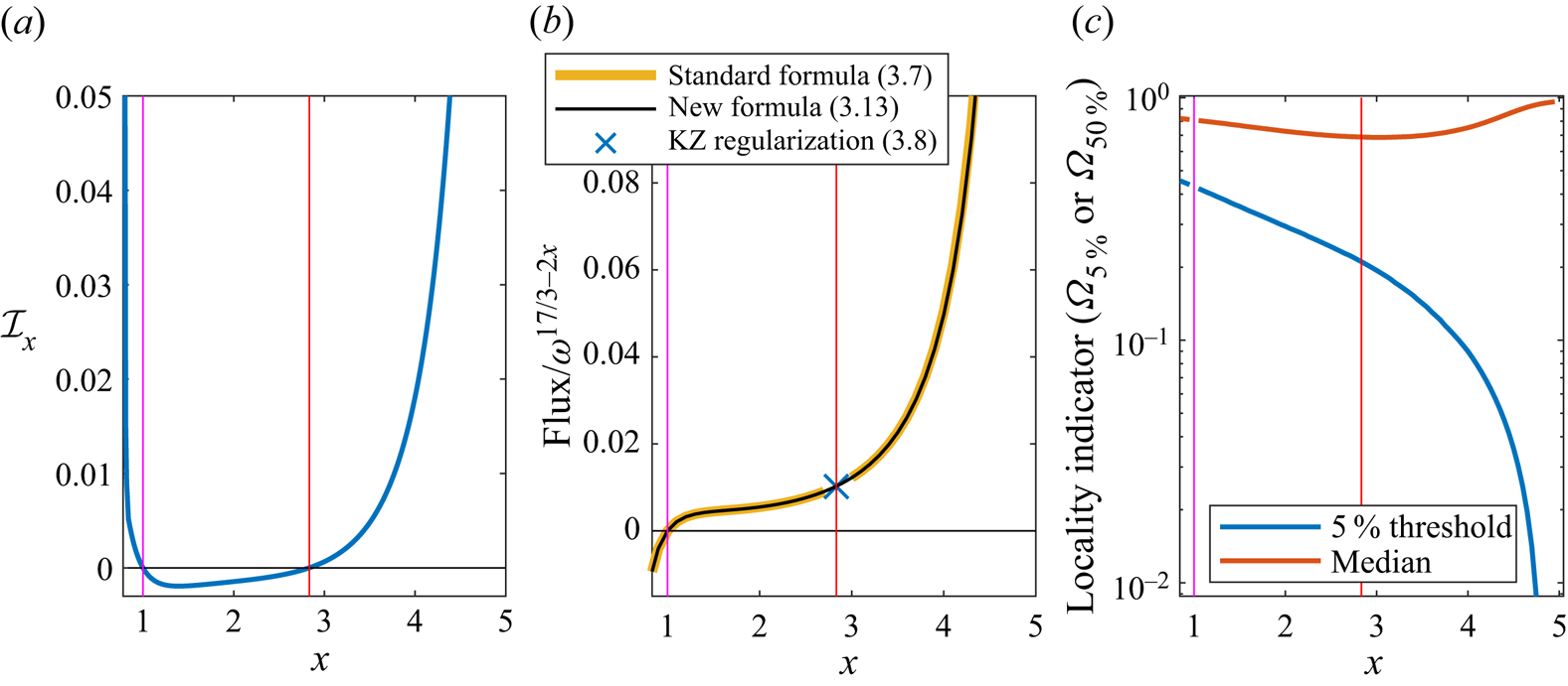
 $[\tfrac 56,5]$, which includes both stationary solutions. For the explicit form of the WKE, we refer the reader to Pushkarev & Zakharov (Reference Pushkarev and Zakharov2000). We perform the analytical calculations of the locality conditions in Appendix C. These calculations are not new per se, as they are implied in Pushkarev & Zakharov (Reference Pushkarev and Zakharov2000). Since we were not able to find these calculations in the literature, we included them here. In figure 2(a), we show a numerical evaluation of the non-dimensional collision integral
 $\mathcal {I}(x)$, vanishing in the two stationary states. In figure 2(b), we show the numerically calculated energy flux between two adjacent sets. This is done in two ways, according to (3.7) and (3.13), showing perfect agreement between the two as proven analytically in (3.16). With the precision adopted, the numerical value so obtained at the KZ solution via (3.13) is identical to the value from the regularization formula (3.8), up to a relative error of the order of
 $1/1000$. Via the inversion (3.20), this value relates directly to the Kolmogorov constant of the capillary wave problem (Pushkarev & Zakharov Reference Pushkarev and Zakharov2000). In the most up-to-date estimates, a direct comparison with the measured flux finds an agreement within a factor around 1.5–2 from numerical simulations of the equations of motion (Deike et al. Reference Deike, Fuster, Berhanu and Falcon2014b; Pan & Yue Reference Pan and Yue2014; Pan Reference Pan2017), and within a factor of approximately 3–4 from experiments (Deike, Berhanu & Falcon Reference Deike, Berhanu and Falcon2014a).
(a) Values of the non-dimensional collision integral  $\mathcal {I}(x)$ as a function of the spectral exponent
 $x$ in the locality interval. The two zeros are the RJ and KZ solutions, indicated by magenta and red vertical lines, respectively. (b) Energy flux normalized by its scaling in
 $\omega$, as a function of
 $x$. The plot shows perfect agreement between the numerical evaluation of the standard flux formula and our formula. Moreover, note that the latter does not need to be regularized at the KZ solution because it does not contain an indeterminate form
 $0/0$, and the result is identical to the regularization by l'Hôpital's rule. (c) We represent the metrics introduced in (4.1a,b) to characterize how local the energy transfers are. All solutions are local for
 $x\in [5/6,5]$, intended as having an integrable collision operator. However, locality as quantified by (4.1a,b) is stronger for small values of
 $x$, increasing as
 $x\to 5$ (where
 $\varOmega _{5\,\%}\to 0$).

Note that the new formula (3.13) can be applied throughout the locality interval, including at the KZ solution, because it does not contain an indeterminate form ‘ $0/0$’, as discussed above. Moreover, the decomposition of the power in terms of the transfer integral (3.19) is now available also for the KZ solution. We point out that the integrand of the regularization formula (3.8), containing a logarithmic function, is not equivalent to the transfer-integral decomposition (3.19). Indeed, only the latter can be used to quantify locality and distant-transport scalings.
4.2. Metrics of locality and distant transport
We next exploit the formalism of § 3.4 to decompose the energy flux based on the relative separation of the frequencies involved in the transport. We define the quantities  $\varOmega _{5\,\%}$ and
 $\varOmega _{50\,\%}$ as
 \begin{align} \int_{0}^{\varOmega_{5\,\%}} {\rm d}\varOmega \,T(\varOmega) := 0.05 \int_{0}^{1} {\rm d}\varOmega \,T(\varOmega) ,\quad \int_{0}^{\varOmega_{50\,\%}} {\rm d}\varOmega \,T(\varOmega) := 0.5 \int_{0}^{1} {\rm d}\varOmega \,T(\varOmega) . \end{align}
The first quantity measures the length of the tail of the transfer integral that contains 5 percent of the total energy transfer. This quantity therefore indicates how far apart two regions in Fourier space have to be for their mutual interactions to be negligible. We define ‘negligible’ to be five per cent of total flux of energy. The second quantity is the median threshold of the transfer integral: half of the energy flux is exchanged within this threshold range, and the other half is exchanged from further than this threshold. Figure 2(c) shows the dependence of  $\varOmega _{5\,\%}$ and
 $\varOmega _{50\,\%}$ on the spectral exponent
 $x$. The median
 $\varOmega _{50\,\%}$ is always quite close to
 $1$, with a minimum around the KZ solution where
 $\varOmega _{50\,\%}\simeq 0.7$. However, the tail metric
 $\varOmega _{5\,\%}$ is decreasing from a value around
 $0.5$ in the neighbourhood of the RJ solution, and tends to zero as
 $x\to 5$. In particular, at the KZ solution we have
 $\varOmega _{5\,\%}\simeq 0.2$. This means that frequencies that are separated by up to more than half a decade are still giving a relevant contribution to direct energy transport in the KZ stationary state!
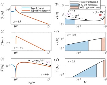
The details of the transfer integral calculations are shown in figure 3, for three different values of  $x$:
 $4.5$,
 $\tfrac {17}{6}$ and
 $0.9$. Figures 3(a,c,e) show the magnitude of the interaction kernel. In the first two cases, the type I contributions are positive and the type II negative, corresponding to a direct cascade. In the final case, the signs are exchanged, corresponding to inverse cascade for
 $x<1$.
Interaction kernel and transfer integral for three different values of  $x$. All plots are in log-log scale. The three solutions here represented are ‘local’: the interaction kernel is integrable. The limiting scalings of the three locality conditions IR, UV1 and UV2 (cf. § 7) are represented by the black dashed lines.

The singularity in  $1$ for large values of
 $x$ behaves like
 $|\omega _1/\omega -1|^{-x+3}$. With the two integrations in (3.17), the convergence condition must be
 $x<5$, retrieving the infrared (IR) locality condition. This implies that the transfer integral is dominated by an integrable singularity
 $T(\varOmega )\simeq (1-\varOmega )^{-x+4}$ for
 $\varOmega \to 1$, when
 $x>4$.
The scaling of the interaction kernel for  $\omega _1/\omega \gg 1$ is given by
 $(\omega _1/\omega )^{-x-1/6}$ for
 $x\simeq 1$, and by
 $(\omega _1/\omega )^{-x-1/3}$ for
 $x\gg 1$. For the transfer integral
 $T(\varOmega )$ to converge, it must have
 $-x-1/6<-1$, which gives the familiar ultraviolet (UV) locality condition
 $x>5/6$. Notice the proximity of the case
 $x=0.9$ to this limit scaling in figure 3(e). By (3.19), this implies an asymptotic scaling
 $T(\varOmega )\simeq {\varOmega ^{4-x}}$ for
 $\varOmega \ll 1$. This will be discussed further in § 7.
Let us use this result to estimate the asymptotic scaling of the distant-transport power:
 \begin{equation} \mathcal{P}_{[0,\tilde\omega]\rightarrow [\omega,+\infty)} = \int_0^{{\tilde\omega}/{\omega}} T(\varOmega)\,{\rm d}\varOmega \sim \left(\frac{\tilde\omega}{\omega}\right)^{5-x},\quad \text{as} \ \frac{\tilde\omega}{\omega} \to 0. \end{equation}
For the KZ solution,  $x=17/6$, this yields
 $\mathcal {P}_{[0,\tilde \omega ]\rightarrow [\omega,+\infty )} \sim ({\tilde \omega }/{\omega })^{13/6}$.
Thus the energy cascade at the KZ stationary solution of capillary waves can be considered quite strongly local; moreover, the energy transport for spectra that are steeper than KZ becomes more and more diffuse, while for whiter spectra, it becomes more and more local (cf. figure 2). Around equilibrium,  $x\simeq 1$, the scaling decay is
 $({\tilde \omega }/{\omega })^{23/6}$. The analysis presented here suggests a viable approach to quantifying how far from the dissipation and forcing regions one should be in order for direct energy transfers with the boundaries to be fairly negligible. Taking
 $\varOmega _{5\,\%}$ as a reasonable (albeit arbitrary) cutoff for a notion of ‘negligibility’, for KZ we would obtain at least a factor of
 $5$ of separation from each boundary. A criterion of this sort would exclude approximately
 $1.4$ orders of magnitude (half on each side) from being a part of an inertial range fairly independent of both the forcing and the dissipation regions. For surface capillary waves, which are constrained on scales from
 $0.5$ mm to
 $17$ mm, there are approximately
 $2.3$ orders of magnitude of available frequencies, which is not much larger than
 $1.4$. We refer the reader to § 7 for further discussion.
These and similar quantifications of fluxes and associated level of locality are applicable directly to any wave turbulence system. They open the possibility to an analysis of energy transfers that goes beyond the mere stationary states to explore transients, boundary effects and a scale-by-scale decomposition of the energy transfer contributions.
5. Anisotropic systems
5.1. Overview on the theory of energy fluxes
A direct extension to anisotropic systems of the theory of energy fluxes reviewed in § 3.1 is possible, in scale-invariant and stationary conditions. It consists of the use of generalized Zakharov–Kraichnan–Kuznetsov conformal transformations (Kuznetsov Reference Kuznetsov1972) to find generalized KZ solutions (Zakharov et al. Reference Zakharov, L'vov and Falkovich1992; Nazarenko Reference Nazarenko2011). Each of these solutions corresponds to the stationary cascade solution of one of the positive-definite conserved quantities of the WKE. In principle, each of these positive invariants also corresponds to an independent equilibrium solution. However, at variance from the isotropic case, these types of equilibrium and non-equilibrium stationary solutions are not the only possible stationary solutions, but only particular ones. In the case of 3-D systems with two effective independent dimensions, there are two families of an infinite number of equilibrium and non-equilibrium solutions, respectively represented by the points of two 1-D curves in the two-dimensional (2-D) plane of possible power-law exponents. Physical examples are the Rossby/drift waves, where there are three positive collision invariants and three KZ solutions (Balk, Zakharov & Nazarenko Reference Balk, Zakharov and Nazarenko1990; Nazarenko Reference Nazarenko2011), or the internal gravity waves, where there is one known collision invariant (the energy) and one corresponding KZ solution (Pelinovsky & Raevsky Reference Pelinovsky and Raevsky1977; Lvov & Tabak Reference Lvov and Tabak2001). Another remarkable recent application is found in Galtier (Reference Galtier2006) and in David & Galtier (Reference David and Galtier2022) to the problem of inertial electron magnetohydrodynamics in plasma physics. One subsequent necessary step in the theory is the verification that these stationary solutions correspond to a convergent collision integral, i.e. that they are local. For internal gravity waves, for instance, there is only one local stationary solution that is found numerically (Lvov et al. Reference Lvov, Tabak, Polzin and Yokoyama2010) and is different from the KZ solution.
The calculation of the fluxes for the anisotropic KZ solutions leads to a regularization similar to (3.7)–(3.8). Here, we make use of simple-minded dimensional analysis to illustrate its properties. For concreteness, we will use the example of horizontally isotropic internal gravity waves. In the hydrostatic approximation, the scale-invariant dispersion relation and matrix elements read (Olbers Reference Olbers1976; Lvov & Tabak Reference Lvov and Tabak2004)
 \begin{equation} \omega_{\boldsymbol{p}} = \gamma\,\frac{k}{m},\quad \left|V_{12}^0\right|^2=V_0^2 k^{2\mu_k}m^{2\mu_m}\, f\left(\frac{k_1}{k},\frac{k_2}{k},\frac{m_1}{m},\frac{m_2}{m}\right), \end{equation}
where  $\gamma$ and
 $V_0$ are dimensional constants, and
 $k$ and
 $m$ are the magnitudes of the (2-D) horizontal and (1-D) vertical wavenumbers, respectively. Moreover, we have
 $\mu _k=3/2$ and
 $\mu _m=-1/2$. In an inertial range where no external forcing or dissipation is present, we look for general stationary solutions for the action density of the form
 \begin{equation} n_{\boldsymbol{p}}=A k^{{-}a} m^{{-}b}. \end{equation}
Let us study energy propagation in the positive quadrant for  $k\unicode{x2013} m$, by defining the horizontally averaged wave action
 $n(k,m)= 4{\rm \pi} k n_{\boldsymbol {p}}$ and energy
 $e(k,m)=\omega _{\boldsymbol {p}} n(k,m)$. The standard use of the differential conservation equation for energy yields
 \begin{equation} \frac{\partial e(k,m)}{\partial t} = 4{\rm \pi} k \omega_{\boldsymbol{p}} I_{\boldsymbol{p}} ={-}\frac{\partial F_k(k,m)}{\partial k} - \frac{\partial F_m(k,m)}{\partial m}, \end{equation}
where the dependence on time is implicit,  $I_{\boldsymbol {p}}$ is the collision integral, and
 $F_k$ and
 $F_m$ are the horizontal and vertical components of the energy flux in
 $k\unicode{x2013} m$ space. Using (5.1)–(5.2), from dimensional analysis we obtain
 \begin{equation} k \omega_{\boldsymbol{p}} I_{\boldsymbol{p}} = (V_0 A)^2 k^{6-2a} m^{{-}2b}\,\mathcal{I}(a,b), \end{equation}
where  $\mathcal {I}(a,b)$ is the non-dimensional collision integral that vanishes in the stationary states. Let us plug this into the right-hand side of (5.3). We follow similar reasoning as for (3.7) in the isotropic case. Let us assume that
 $F_k=F_k(m)$ and
 $F_m=F_m(k)$ – a posteriori, the KZ solution is found to enjoy this property. Under this assumption, we integrate in
 $k$ from
 $0$ to
 $k$ to obtain the horizontal component of the flux, and in
 $m$ from
 $0$ to
 $m$ to obtain the vertical component. We obtain
 \begin{align} F_k ={-}4{\rm \pi}(V_0 A)^2\,\frac{k^{7-2a}m^{{-}2b}}{7-2a}\,\mathcal{I}(a,b),\quad F_m ={-}4{\rm \pi} (V_0 A)^2\,\frac{k^{6-2a}m^{1-2b}}{1-2b}\,\mathcal{I}(a,b). \end{align}
Using the generalized Zakharov–Kraichnan–Kuznetsov transformations, one finds that the generalized KZ solution is the particular one for which the above denominators vanish (Lvov & Tabak Reference Lvov and Tabak2001), setting  $a_{KZ}=7/2$,
 $b_{KZ}=1/2$, the Pelinovsky–Raevsky spectrum (Pelinovsky & Raevsky Reference Pelinovsky and Raevsky1977). Because for this solution also the numerators vanish, in analogy with (3.8), one can regularize the
 $0/0$ indeterminate form by l'Hôpital's rule to obtain (Zakharov et al. Reference Zakharov, L'vov and Falkovich1992)
 \begin{equation} F_k^{KZ} = 2{\rm \pi} (V_0A)^2{m^{{-}1}}\left.\frac{\partial\mathcal{I}}{\partial a}\right|_{(a_0,b_0)},\quad F_m^{KZ} =2{\rm \pi} (V_0A)^2{k^{{-}1}}\left.\frac{\partial \mathcal{I}}{\partial b}\right|_{(a_0,b_0)}. \end{equation}
Notice that the KZ solution is the particular case for which the  $k$-component is independent of
 $k$, i.e.
 $F_k=F_k(m)$, and the
 $m$-component is independent of
 $m$, i.e.
 $F_m=F_m(k)$. This spectrum is known to be non-local (Lvov et al. Reference Lvov, Tabak, Polzin and Yokoyama2010). In particular, the point
 $(\tfrac 72,\tfrac 12)$ in the
 $a\unicode{x2013} b$ plane exhibits divergences at both high and low wavenumbers. These divergences can also be seen from (5.6a,b): integrating the flux along any boundary in
 $k\unicode{x2013} m$ space yields a logarithmic divergence both at low wavenumbers (
 $k\to 0$,
 $m\to 0$) and at large wavenumbers (
 $k\to \infty$,
 $m\to \infty$). Thus (5.6a,b) can be written only in a formal way, but in practice they have no meaning. It was shown in Lvov et al. (Reference Lvov, Tabak, Polzin and Yokoyama2010) that there is only one stationary solution that is local, with spectral exponent values
 $a=3.69$,
 $b=0$. However, for this non-KZ stationary solution, (5.3) is merely stating that the divergence of the flux is zero. Therefore, it is possible to determine only the direction of the flux, but the magnitude of the flux of energy remains undetermined. This is shown in Appendix D.
6. Anisotropic illustration: internal gravity waves
6.1. Definition of the problem
Here, we illustrate an application of (2.1) to the anisotropic problem of internal gravity waves (Olbers Reference Olbers1976; Caillol & Zeitlin Reference Caillol and Zeitlin2000; Lvov & Tabak Reference Lvov and Tabak2004). This is non-trivial in several ways, involving: (i) physically motivated control volumes in Fourier space with a geometry that is more interesting than simple rectangles in  $k\unicode{x2013} m$ space; (ii) a relevant stationary spectrum that is not a KZ solution (the solution
 $a=3.69$,
 $b=0$); (iii) a renowned spectrum (the Garrett–Munk spectrum) that is not stationary under the wave kinetic equation evolution; (iv) decomposition of the fluxes in terms of transfer integrals allowing us to quantify the level of locality. Each of these points could not be analysed fully by the standard wave turbulence theory of energy fluxes summarized in § 5. These results were obtained intuitively in Dematteis & Lvov (Reference Dematteis and Lvov2021) and Dematteis, Polzin & Lvov (Reference Dematteis, Polzin and Lvov2022). Here, we provide firm mathematical justification for results of such a type, study locality of internal wave interactions, and analyse the celebrated Garrett–Munk spectrum.
The boundaries in spectral space are defined naturally for internal waves. The frequency  $\omega$ takes values in the interval
 $[f,N]$, where
 $f$ and
 $N$ are the inertial and buoyancy frequencies, respectively. These two frequencies give the minimal and maximal frequencies (
 $f\ll N$) of the problem, with the inertial range between them. The vertical wavenumber
 $m$ takes values in
 $[m_{min},m_{max}]$, where
 $m_{min}=2{\rm \pi} /H$,
 $m_{max}=2{\rm \pi} /h$, with
 $H$ and
 $h$ being the ocean depth and the vertical scale past which internal waves become unstable due to shear instability. Let us assume that the box
 $\mathcal {A}=[f,N]\times [m_{min},m_{max}]$ is the inertial range, and for
 $m>m_{min}$ and
 $\omega >N$, strong turbulence acts as an idealized sink. Suitable energy sources will indeed be necessary at the bottom and left boundaries of the ‘inertial box’
 $\mathcal {A}$, in order for an energy cascade to be sustained in time. The inertial box
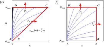
 $\mathcal {A}$ is shown in figure 4, in both
 $k\unicode{x2013} m$ space and
 $\omega \unicode{x2013} m$ space. The change of variables between the two spaces is prescribed by the dispersion relation (5.1). In figure 4, we also show the streamlines of the energy flux obtained by dimensional arguments in Appendix D, namely (D1a,b), for the stationary state with
 $a=3.69$,
 $b=0$. These lines give a sense of the need for a source at low frequencies and low wavenumbers for energy to be delivered to the whole inertial box. We use
 $\mathcal {A}$ as our input control volume. For the output control volume,
 $\mathcal {B}$, we consider two possibilities: either
 $\mathcal {B}_{h}=\{(\omega,m): \omega >N\}$ or
 $\mathcal {B}_{v}=\{(\omega,m): m>m_{max}\}$. In the first case, the power
 $\mathcal {P}_{\mathcal {A}\rightarrow \mathcal {B}}$ defines the quantity
 $\mathcal {P}_{h}$, the instantaneous power transferred ‘horizontally’ through the boundary denoted as
 $BC$ in figure 4. In the second case,
 $\mathcal {P}_{\mathcal {A}\rightarrow \mathcal {B}}$ defines the quantity
 $\mathcal {P}_{v}$, the instantaneous power transferred ‘vertically’ through the boundary denoted as
 $CD$. The powers
 $P_{h}$ and
 $P_{v}$ are calculated rigorously in the next subsection using the main statement (2.1).
Representation of the 2-D Fourier space for the anisotropic internal-wave problem: (a) in horizontal–vertical wavenumber  $k\unicode{x2013} m$ coordinates; (b) in frequency–vertical wavenumber
 $\omega \unicode{x2013} m$ coordinates. The streamlines represent the energy flux vector field and are drawn from (D1a,b) for the stationary solution
 $a=3.69$,
 $b=0$. Equation (D1a,b) is determined up to an arbitrary factor
 $C$, but this nonetheless allows us to know the flux direction (thus the streamlines). The change of coordinates from the
 $k\unicode{x2013} m$ to the
 $\omega \unicode{x2013} m$ representation is given by the dispersion relation (5.1). The quantities
 $P_{h}$ and
 $P_{v}$ are computed rigorously in (6.1a,b). The computations in this paper are performed in
 $k\unicode{x2013} m$ space, although the physical boundaries are defined naturally in
 $\omega \unicode{x2013} m$ space. This figure illustrates the equivalence between the two representations.

6.2. Application of the main statement (2.1) and transfer integrals
Applying (2.1), we obtain (Dematteis & Lvov Reference Dematteis and Lvov2021)
 \begin{equation} \mathcal{P}_{h} = \int_{m_{min}}^{m_{max}} {\rm d}m \,\mathcal{F}_{h}(m), \quad \mathcal{P}_{v} = \int_{({f}/{\gamma})m_{max}}^{({N}/{\gamma})m_{max}} {\rm d}k \,\mathcal{F}_{v}(m), \end{equation}
where
 \begin{gather} \mathcal{F}_{h}(m) =\frac{N^2}{g}\,(V_0A)^2 \left(\frac{N}{\gamma}\,m\right)^{7-2a}m^{{-}2b} \int_{{f}/{N}}^{1}{\rm d} K \,T_{h}(K), \end{gather}
 \begin{gather} T_{h}(K)={-}\frac{4{\rm \pi} }{ (V_0A)^{2}}\,K^{6-2a} \int {\rm d}\xi_1\,{\rm d}\xi_2 \sum_l \chi_{K}^{(l)}(\xi_1,\xi_2)\,J^{({ l})}(\xi=1, \mu=1;\xi_1,\xi_2) \end{gather}
and
 \begin{gather} \mathcal{F}_{v}(k) =\frac{N^2}{g}\,(V_0A)^2 k^{6-2a} m_{max}^{1-2b} \int_{{m_{min}}/{m_{max}}}^{1} {\rm d} M \,T_{v}(M), \end{gather}
 \begin{gather} T_{v}(M)={-}\frac{4{\rm \pi} }{(V_0A)^{2}}\,M^{{-}2b} \int {\rm d}\xi_1\,{\rm d}\xi_2 \sum_l \chi_{M}^{(l)}(\xi_1,\xi_2)\,J^{({ l})}(\xi=1, \mu=1;\xi_2,\xi_2). \end{gather}
Here,  $J^{({ l})}(\xi =1, \mu =1;\xi _1,\xi _2)$ denotes the six resonant branches of the interaction kernel corresponding to the triad of non-dimensional horizontal wavenumbers
 $\xi =1$,
 $\xi _1=k_1/k$,
 $\xi _2=k_2/k$, and vertical wavenumber
 $\mu =1$. The six resonant conditions determine the values of
 $\mu _1=m_1/m$ and
 $\mu _2=m_2/m$. The characteristic interaction weights
 $\chi _K^{({ l})}(\xi _1,\xi _2)$ are defined by the rules in table 1, taking
 $\mathcal {B}_{h}=\{\xi :\xi >K^{-1}\}$, with
 $K^{-1}>1$. The weights
 $\chi _M^{({ l})}(\xi _1,\xi _2)$ are defined likewise by taking
 $\mathcal {B}_{v}=\{\mu :\mu >M^{-1}\}$, with
 $M^{-1}>1$, where the condition
 $\mu >M^{-1}$ is applied to the non-dimensional vertical wavenumbers
 $\mu _1$ and
 $\mu _2$ found as solution of the
 $l$th resonant branch.
Using similar equations, it was shown in Dematteis & Lvov (Reference Dematteis and Lvov2021) and Dematteis et al. (Reference Dematteis, Polzin and Lvov2022) that both the scaling and the prefactor of the total calculated power are in order-of-magnitude agreement with the observational fine-scale parametrization of oceanic turbulent production (Polzin et al. Reference Polzin, Garabato, Huussen, Sloyan and Waterman2014), up to a factor  $1.5$ difference. In a loose sense, these calculations are equivalent to evaluating the Kolmogorov constant for the internal wave problem, i.e. expressing the explicit theoretical relationship between the energy flux and the spectral energy density.
6.3. Metrics of locality and distant transport
The methodology developed in this paper allows us not only to compute the fluxes of energy, but also to analyse the locality of interactions. In relation to their isotropic version (3.18)–(3.19), indeed the expressions (6.1a,b)–(6.5) feature one extra integration along the boundaries of the 2-D inertial box. The quantities  $\mathcal {F}_{v}(k)$ and
 $\mathcal {F}_{h}(m)$ are energy fluxes per unit of
 $k$ and
 $m$, respectively. Thanks to scale invariance, their dependence on
 $k$ and
 $m$ is given by the scaling relations in (6.2) and (6.4). Therefore, to study level of locality of the interactions, it is sufficient to study
 $\mathcal {F}_{v}(k=1)$ and
 $\mathcal {F}_{h}(m=1)$, whose structure is expressed in terms of the transfer integrals
 $T_{h}$ and
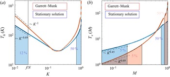
 $T_{v}$ in (6.3) and (6.5). This is represented in figure 5. For both
 $T_{h}$ and
 $T_{v}$, the further from the boundary at
 $K=1$ or
 $M=1$, the more non-local (i.e. with large-scale separation) the contribution to the energy transfer. The dashed coloured lines at the right of each plot indicate the analytical leading orders (integrable singularities) from the IR region of the resonant manifold. The scalings on the left side are given by the UV leading orders, multiplied by the factor in (6.3) and (6.5). The shaded areas indicate the leftmost and rightmost contributions to the total flux, in a percentage amount indicated in the figure. Two different spectra in the form (5.2) are studied below (Lvov et al. Reference Lvov, Tabak, Polzin and Yokoyama2010).
(i)
 $a=3.69$, $b=0$ (stationary state of the internal WKE).
For the horizontal transport, despite having the rightmost
$50\,\%$ coming from the $[0.7,1]$ interval (i.e. the median is approximately $0.7$), the heavy tail implies that approximately $12\,\%$ of the power $\mathcal {P}_{h}$ is transferred directly from modes that are smaller than the left boundary of the inertial box, i.e. $\omega < f$ – if we take $N/f=40$, then we obtain a realistic oceanic aspect ratio. Since there are no waves at $\omega < f$, this is not possible. Nevertheless, it indicates that the horizontal transfer is highly non-local – even though the spectrum is ‘local’ in terms of convergence of the collision integral. Even the lowest frequencies in the system are connected energetically with the dissipation region at high frequency in a non-negligible way.For the vertical transport, the situation is much more local. The median is around
$0.8$, and the rightmost $5\,\%$ of the energy transfer comes from the left of approximately $0.2$. Because a realistic range of vertical scales varies by a factor of the order of $200$, a factor $5$ of distance from the boundary at $m_{max}$ is relatively quite small. Thus the vertical transport is highly local.(ii)
$a=4$, $b=0$ (scale-invariant limit of the Garrett–Munk spectrum).The horizontal transport power is marginally divergent, due to a
$K^{-1}$ singularity as $K\to 0$. Therefore, it is not meaningful to indicate percentage metrics of the contribution.The vertical transport is highly local, more so than for the stationary spectrum. Approximately
$95\,\%$ of the total power $\mathcal {P}_{v}$ comes from the region within a factor $3$ from the dissipation boundary.


Let us exploit the transfer integrals to define the distant-transport fluxes, neglecting the dimensional prefactors
 \begin{equation} \left. \begin{aligned} & \mathcal{F}_{{h},[0,\tilde\omega]\rightarrow [\omega,+\infty)} \propto \int_{0}^{\tilde\omega/\omega} {\rm d}K \,T_{h}(K),\\ & \mathcal{F}_{{v},[0,\tilde m]\rightarrow [m,+\infty)} \propto \int_{0}^{\tilde m/m} {\rm d} M \,T_{v}(M). \end{aligned} \right\} \end{equation}
For horizontal transport, we know the analytical scaling  $T_{h}(K)\propto K^{3-a}$ as
 $K\to 0$ (cf. figure 5a). This means that we have
 $\mathcal {F}_{{h},[0,\tilde \omega ]\rightarrow [\omega,+\infty )}\propto ({\tilde \omega }/{\omega })^{4-a}$ as
 ${\tilde \omega }/{\omega }\to 0$. This shows that the flux for the Garrett–Munk spectrum is marginally divergent (logarithmic divergence), and that the stationary spectrum has a very weak decay with scaling
 $({\tilde \omega }/{\omega })^{0.31}$. For vertical transport, we use the numerical scalings shown in figure 5(b). These imply for
 $\mathcal {F}_{{v},[0,\tilde m]\rightarrow [m,+\infty )}$, a scaling
 $({\tilde m}/{m})^{1.69}$ for the Garrett–Munk spectrum, and a scaling
 $({\tilde m}/{m})^{1.45}$ for the stationary spectrum.
We end the section by showing that even when a solution is mathematically non-local, a regularization takes place if one considers physical cutoffs. For the high wavenumber limit of the Garrett–Munk spectrum, indeed a fairly plausible oceanic condition (Pollmann Reference Pollmann2020; Le Boyer & Alford Reference Le Boyer and Alford2021; Thakur et al. Reference Thakur, Arbic, Menemenlis, Momeni, Pan, Peltier, Skitka, Alford and Ma2022), the integral defining the horizontal energy flux has a logarithmic divergence (considering an idealized zero minimal frequency). However, real physical systems have boundaries and other constraints that imply natural lower and upper cutoffs in Fourier space. For instance, oceanic internal waves cannot oscillate at frequencies lower than the Coriolis frequency  $f$. Imposing this lower cutoff by hand, the horizontal flux in (6.6) is given by
 \begin{equation} \mathcal{F}_{{h},[f,\tilde\omega]\rightarrow [\omega,+\infty)} \propto \int_{f/\omega}^{\tilde\omega/\omega} {\rm d}K \,K^{3-a}\propto \frac{1}{4-a}\,\frac{\tilde\omega^{4-a} - f^{4-a}}{\omega^{4-a}}. \end{equation}
For a given frequency  $\tilde \omega >f$, the flux is finite and continuous in
 $a$, with
 $\lim _{a\to 4^{\pm }}\mathcal {F}_{{h},[f,\tilde \omega ]\rightarrow [\omega,+\infty )}=|{\log (f/\omega )}|$. For
 $a\ll 4$, the contribution to the flux from
 $[f,\tilde \omega ]$ is concentrated around
 $\tilde \omega$. As
 $a\to 4^-$, the contribution becomes less and less concentrated in
 $\tilde \omega$. For
 $a>4$, the contribution becomes more concentrated in
 $f$ than in
 $\tilde \omega$, and increasingly so as
 $a$ increases. Since the non-locality and boundary dependence are smooth functions of
 $a$, and the transition is continuous in
 $a=4$, it is clear that interpreting this threshold as a sharp definition of physical realizability/non-realizability is quite fictitious. For a physical system with a finite available range of scales, highly non-local spectra will indeed show strong dependence on the boundaries, as (6.7) demonstrates. If the forcing is varying strongly in time, for instance, this will correspond to transient forcing-driven conditions, with the system being influenced highly by the forcing variability at the lower boundary of Fourier space. However, it may still be of fundamental importance to quantify the associated energy fluxes: the energy fluxes associated with highly non-local and transient spectra of internal waves play a crucial role for the oceanic circulation and climate at large (Polzin et al. Reference Polzin, Garabato, Huussen, Sloyan and Waterman2014).
7. Integrability conditions and locality of energy transport
Here, we consider the conditions for a finite energy transfer and discuss their consistency with the standard locality conditions of wave turbulence (Zakharov et al. Reference Zakharov, L'vov and Falkovich1992). Moreover, we suggest a way to quantify the locality properties of a wave turbulence spectrum.
Consider a generic isotropic system with distant-transport power described by (3.18)–(3.19). Defining  $f(\xi )=J^{(\textrm {II})}(1;\xi,\xi -1)$, assume the following definitions for the scaling exponents
 $\gamma _0,\gamma _1,\gamma _2, y$:
 \begin{equation} \left. \begin{aligned} & J^{({\rm II})}(k;k_1,k_1-k) = k^{\gamma_0-2x}\,f\left(\frac{k_1}{k}\right),\quad y = \gamma_0+2-2x,\\ & f(\xi) \propto \xi^{\gamma_2-x} \ \text{as }\xi\to+\infty,\quad f(\xi)\propto (\xi-1)^{\gamma_1-x}\ \text{as }\xi\to1^+. \end{aligned} \right\} \end{equation}
For the distant-power (3.18) to be finite for any  $\tilde \omega \in [0,\omega ]$, we have to impose the integrability of
 $T(\varOmega )$ defined by (3.19), in the integration domain
 $[0,\omega ]$. Setting the prefactor to unity for simplicity, we recall that
 \begin{equation} \mathcal{P}_{[0,\omega]\rightarrow [\omega,+\infty)} = \omega^{y+1} \int_{0}^{1} {\rm d}\varOmega \,T(\varOmega), \quad T(\varOmega)= \varOmega^{y} \int_{\varOmega^{{-}1}}^{+\infty} {\rm d}\xi \, f(\xi). \end{equation}
Integrability for  $\varOmega \to 1$, due to double integration, gives the Zakharov et al. (Reference Zakharov, L'vov and Falkovich1992) IR condition
 \begin{equation} x<\gamma_1+2. \end{equation}
Integrability of  $f(\xi )$ for
 $\xi \to +\infty$ gives the Zakharov et al. (Reference Zakharov, L'vov and Falkovich1992) UV condition (UV1)
 \begin{equation} x>\gamma_2+1. \end{equation}
Now, we have a third condition from integrability of  $T(\varOmega )$ for
 $\varOmega \to 0$. This is also a UV condition (UV2), and reads
 \begin{equation} x<2+\gamma_0-\gamma_2. \end{equation}
For a scale-invariant spectrum  $n_{\boldsymbol {p}}=A\omega ^{-x}$, the instantaneous power exchanged between the sets
 $[0,\omega ]$ and
 $[\omega,+\infty )$ is finite if and only if the three conditions (7.3) (IR), (7.4) (UV1) and (7.5) (UV2) are fulfilled simultaneously. This result needs to be compared with the standard locality conditions of wave turbulence theory (Zakharov et al. Reference Zakharov, L'vov and Falkovich1992; Nazarenko Reference Nazarenko2011), which consist of (7.3) (IR) and (7.4) (UV1). Let us use the example of the capillary wave system, where we have
 $\gamma _1=3$,
 $\gamma _0=8/3$,
 $\gamma _2=-1/6$ for
 $x<1$, and
 $\gamma _2=-1/3$ for
 $x>1$. We provide a detailed calculation of these scalings in Appendix C. The three convergence conditions give
 $x<5$,
 $x>5/6$,
 $x<5$, respectively. The three conditions are represented by the three black dashed lines in figure 3. As we see, for the case of capillary waves, the third condition is identical to the first one, showing that the integrability interval computed by imposing a finite energy transport is fully consistent with the usual locality conditions. Therefore, for the wave turbulence spectrum of any wave turbulence system to be truly local, all of these three locality conditions need to be individually checked and verified.
Using the quantities defined in § 4.2, we propose the definition of a non-dimensional number that quantifies the width of direct energy transport in Fourier space:
 \begin{equation} w ={-}\log_{10}\varOmega_{5\,\%}, \end{equation}
in units of orders of magnitude. This quantity is a measure of the inter-scale width of the resonant interactions. If, for example, this quantity tends to zero, then it means that the interactions are highly local. If this quantity is comparable to the range of scales that are physically available, then there cannot exist an inertial range of scales where the interactions are sufficiently independent of the boundaries. This quantity diverges for spectra outside the locality interval. Using the power-law tail scaling  $T(\varOmega )\sim c\varOmega ^{1+\gamma _0-\gamma _2-x}$ as
 $\varOmega \to 0$, and the definition (4.1a,b), we obtain the estimate
 \begin{equation} w = (x-2-\gamma_0+\gamma_2) \log_{10}\left(\frac{0.05}{c}(2+\gamma_0-\gamma_2-x)\int_0^1 T(\varOmega)\,{\rm d}\varOmega\right). \end{equation}
In the examples illustrated in this paper (cf. figures 3 and 5), we have  $w\simeq 0.3$ near equilibrium, and
 $w\simeq 0.7$ at the KZ solution of surface capillary waves. For the horizontal transport of internal waves, we have
 $w\simeq 2.1$ for the stationary solution, and
 $w\to \infty$ for the Garrett–Munk scale-invariant limit (logarithmic divergence). For vertical transport, we have
 $w\simeq 0.7$ for the stationary solution and
 $w\simeq 0.5$ for the Garrett–Munk spectrum of internal waves. We can see that
 $w$ is finite if
 $x$ is in the locality interval. However, its value can vary from close to zero, when transport is highly local, to fairly large values, even if the spectrum is ‘local’ (see e.g. horizontal transport for internal waves in § 6). The estimate of
 $w$ can be important for understanding how wide the inertial range of wave turbulence must be in the experiments, in order to become independent of the boundaries.
8. Discussion
We introduced (2.1) for systematic computation of any inter-scale energy transfers in a system governed by a WKE with three-wave resonances. For isotropic systems, in § 3 we showed rigorously that the formula encompasses the standard formula (3.7) for the energy flux as a particular case of adjacent control volumes in Fourier space (cf. (3.16)). Using the property of detailed energy conservation (3.14), we showed that the standard flux formula contains a vanishing part corresponding to self-interactions (cf. (3.15)). The new formula always allows us to compute inter-scale energy fluxes as integrals of non-zero quantities, also in the stationary states – except, naturally, for equilibrium states for which the interaction kernel is vanishing. This provides a general way to obtain the Kolmogorov constant for a three-wave system. In the isotropic case, it is an alternative route to the KZ regularization (3.8) (cf. figure 2). For anisotropic systems, this paves the way to the computation of energy fluxes, including their prefactors, as shown in § 6.2.
We have formalized the theoretical framework that descends from (2.1) with particular emphasis on the definition of the transfer integral (cf. (3.19), (6.3) and (6.5)). The transfer integral is a decomposition with respect to the scale separation of the instantaneous energy transfers between a mode and a control volume in Fourier space. Using this formalism, we reframed the so-called locality conditions of wave turbulence explicitly in terms of convergence conditions of the energy transfer. In § 7, we showed that the IR and UV convergence conditions for the collision integral, (7.3)–(7.4), are not sufficient to ensure convergence of the energy flux. A third condition (7.5) must be imposed. For the capillary wave turbulence, the third condition appears to be redundant.
Via the transfer integral, we are able to express the power exchanged between distant control volumes in Fourier space and the scaling of the power as a function of the scale separation (cf. (4.2) and (6.6)). This is an important effective metric for the quantification of the locality level of energy transport (Kraichnan Reference Kraichnan1959), which goes beyond establishing a binary local/non-local status of the system. To this end, we have defined a non-dimensional number  $w$, the interaction width in Fourier space. Given a closed set of modes
 $B$ in Fourier space, the number
 $w$ quantifies how far away from set
 $B$ one has to move in order to include the
 $95\,\%$ fraction of the total power transferred to
 $B$ via resonant interactions. Equivalently,
 $w$ quantifies the distance in Fourier space past which the farthest (i.e. most scale-separated)
 $5\,\%$ of the contribution to the energy transfer to
 $B$ is confined. The width
 $w$ is thus defined naturally in terms of a definite integral of the transfer integral. The
 $5\,\%$ threshold is chosen arbitrarily as a means to roughly establish a negligibility threshold. Moreover, to emphasize the meaning of scale separation of the energy transfer, we defined
 $w$ in logarithmic scale. As an example, consider
 $B$ as the set of all the modes larger than a value
 $k$. A value
 $w=1$ would mean that
 $95\,\%$ of the energy transferred to
 $B$ from modes smaller than
 $k$ comes from the interval
 $[k/10,k]$, and
 $5\,\%$ comes from
 $[0,k/10]$. According to our definition, the ‘width’ of the energy transfer would then be of one order of magnitude, or a factor of
 $10$.
We have also shown that the link between  $w$ and the standard notion of locality and non-locality is quite direct: for a local spectrum
 $w$ is finite, whereas for a non-local spectrum,
 $w$ is infinite. For local spectra, the value of
 $w$ gives an indication on the range of scales that is necessary if one hopes to observe a wave turbulence cascade. This opens the possibility of estimating theoretically the width of the transition region between the inertial range and the dissipation and forcing regions (cf. §§ 4.2 and 6.2), improving the current understanding of the realizability conditions of KZ spectra. We believe quantifications in this vein to be relevant for experiments of wave turbulence, where the range of available scales is limited, and it is important to evaluate whether the scale separation between the forcing and the dissipation regions is sufficiently large for the onset of an in-between inertial range (Deike et al. Reference Deike, Berhanu and Falcon2014a; Hassaini et al. Reference Hassaini, Mordant, Miquel, Krstulovic and Düring2019; Davis et al. Reference Davis, Jamin, Deleuze, Joubaud and Dauxois2020; Monsalve et al. Reference Monsalve, Brunet, Gallet and Cortet2020; Rodda et al. Reference Rodda, Savaro, Davis, Reneuve, Augier, Sommeria, Valran, Viboud and Mordant2022). In the examples considered in this paper, we have obtained values of
 $w$ of approximately
 $0.3$ near equilibrium and
 $0.7$ at the KZ solution for the surface capillary waves. For internal waves, there are two directions for energy transfers: horizontally, we have
 $w\simeq 2.1$ for the stationary solution and
 $w\to \infty$ for the Garrett–Munk scale-invariant limit (logarithmic divergence); vertically, we have
 $w\simeq 0.7$ for the stationary solution and
 $w\simeq 0.5$ for the Garrett–Munk spectrum of internal waves.
For the isotropic example of surface capillary waves, where there are approximately two orders of magnitude of total available frequencies, our results imply that for the KZ solution, an independent inertial range should have approximately a factor of  $5$ separation between both the forcing and the dissipation regions. Therefore, one is likely to observe a proper wave turbulence solution associated with the KZ solution over a window of less than a decade of width in the frequency domain.
Then the more complex anisotropic example of oceanic internal waves was chosen to show the potential of applicability of our method based on the main statement (2.1). In particular, the method expands our capability to calculate energy fluxes in several ways: (i) for stationary solutions that differ from the KZ solution (as shown for the solution  $a=3.69$,
 $b=0$); (ii) for non-stationary transient solutions (as shown for the scale-invariant regime of the Garrett–Munk spectrum); (iii) for solutions that are mathematically non-local, but after regularization by a physical cutoff are associated with a finite energy flux that is important to quantify (albeit with strong dependence on the cutoff itself; this was also shown for the Garrett–Munk spectrum); (iv) the method applies also to systems that do not satisfy scale invariance.
In summary, we have the following.
(i) We have calculated the amount of energy exchanged between two disjoint sets of wavenumbers in Fourier space. This amount is given by the main statement in § 2 and (2.1).
(ii) We have re-derived the classical formula (3.7) for the flux of energy in scale-invariant isotropic systems. The classical formula needs to be regularized for the KZ stationary state by l’Hôpital's rule, as it has a
$0/0$ indeterminacy.(iii) Our formalism applies to a more general case: non-scale-invariant, not isotropic, not necessarily stationary cases. The formula for the energy fluxes does not need to be regularized as it is a well defined integral of a non-zero quantity.
(iv) Our formalism allows us to characterize the level of locality of a system, by use of what we defined as the transfer integral.
(v) We therefore introduced the number
$w$, (7.6), which characterizes how many orders of magnitude of separation in Fourier space are necessary for two sets of modes to not be exchanging energy directly.(vi) The values of
$w$ calculated in this paper show that a fair amount of ‘teleportation’ in Fourier space is present also in applications where the transport is traditionally considered fully local. We believe that the estimate of $w$ is important for the interpretation of wave turbulence experiments.(vii) The example of surface capillary waves was used to illustrate the application of the main statement (2.1) and the formalism of the transfer integral to a well-known wave turbulence problem.
(viii) We have shown how the transfer integral relates to the Kolmogorov constants of wave turbulence (cf. (3.20)). This equation reveals the ‘inter-scale structure’ of the Kolmogorov constant.
(ix) We have applied our formalism to the anisotropic problem of the internal waves in the ocean.


In conclusion, the formalism presented here allows quantification of instantaneous energy fluxes for wave turbulence systems dominated by three-wave resonant interactions. Our formalism does not require stationarity, scale invariance, or strict fulfillment of the locality conditions. The possible applications of our formalism include the improvement and development of a first-principles understanding of many geophysical wave systems, with possible far-reaching implications for weather and climate prediction.
Acknowledgements
Discussions with Kurt Polzin and Nick Salvatore are gratefully acknowledged. We are thankful to Sergey Nazarenko and two anonymous reviewers for their insightful comments, which helped us to improve significantly the clarity of the paper.
Funding
This research was supported by the NSF DMS award 2009418 and by the ONR grant N00014-17-1-2852.
Declaration of interests
The authors report no conflict of interest.
Appendix A
A.1. Proof of the detailed energy conservation property (1.5)
Using the definition in (1.1), we have
 \begin{align} {\mathcal{Z}}(\boldsymbol{p}_{a},\boldsymbol{p}_b,\boldsymbol{p}_c)&= \omega_a\,(\mathcal{R}^a_{bc} - \mathcal{R}^b_{ca} - \mathcal{R}^c_{ab}) + \omega_b\, (\mathcal{R}^b_{ca} - \mathcal{R}^c_{ab} - \mathcal{R}^a_{bc}) + \omega_c\,(\mathcal{R}^c_{ab} - \mathcal{R}^a_{bc} - \mathcal{R}^b_{ca})\nonumber\\ & =(\omega_a-\omega_b-\omega_c) \mathcal{R}^a_{bc} + (\omega_b-\omega_c-\omega_a) \mathcal{R}^b_{ca} + (\omega_c-\omega_a-\omega_b) \mathcal{R}^c_{ab} . \end{align}
Since  $\mathcal {R}^a_{bc}$ contains
 $\delta (\omega _a-\omega _b-\omega _c)$,
 $\mathcal {R}^b_{ca}$ contains
 $\delta (\omega _b-\omega _c-\omega _a)$ and
 $\mathcal {R}^c_{ab}$ contains
 $\delta (\omega _c-\omega _a-\omega _b)$, each of the three terms vanishes identically (indeed, in the sense of distributions), proving (1.5).
A.2. Proof of the main statement (2.1)
In the following, we provide a proof of the main statement (2.1) in three steps.
A.2.1. Step 1
Consider a triad of type I with two wavenumbers  $\boldsymbol {p}_1$ and
 $\boldsymbol {p}_2$ interacting to generate
 $\boldsymbol {p}$, for which (2.2) holds. This relation has a meaning of energy conservation restricted to the particular triad
 $\boldsymbol {p}, \boldsymbol {p}_1,\boldsymbol {p}_2$ (or detailed energy conservation). Note that for the action rate of wavenumber
 $\boldsymbol {p}$ we have
 \begin{equation} \dot n_{\boldsymbol{p}}|_{012}= \mathcal{J}(\boldsymbol{p};\boldsymbol{p}_1,\boldsymbol{p}_2)=\mathcal{R}^0_{12}-\mathcal{R}^1_{02}-\mathcal{R}^2_{01}=\mathcal{R}^0_{12}, \end{equation}
since  $\mathcal {R}^1_{02}$ and
 $\mathcal {R}^2_{01}$ are vanishing for
 $\omega _{\boldsymbol {p}}=\omega _1+\omega _2$. For the action rate of wavenumber
 $\boldsymbol {p}_1$ we have
 \begin{equation} \dot n_1|_{012}= \mathcal{J}(\boldsymbol{p}_1;\boldsymbol{p},\boldsymbol{p}_2)=\mathcal{R}^1_{02}-\mathcal{R}^0_{12}-\mathcal{R}^2_{01}={-}\mathcal{R}^0_{12}={-}\dot n_{\boldsymbol{p}}|_{012}. \end{equation}
Finally, for the action rate of wavenumber  $\boldsymbol {p}_2$, we have
 \begin{equation} \dot n_2|_{012}= \mathcal{J}(\boldsymbol{p}_2;\boldsymbol{p},\boldsymbol{p}_1)=\mathcal{R}^2_{01}-\mathcal{R}^0_{12}-\mathcal{R}^1_{02}={-}\mathcal{R}^0_{12}={-}\dot n_{\boldsymbol{p}}|_{012}. \end{equation}
Therefore,  $x$ amount of action with energy
 $\omega _1x$ interacts with
 $x$ amount of action with energy
 $\omega _2x$, producing
 $x$ amount of action with energy
 $\omega _{\boldsymbol {p}} x = (\omega _1+\omega _2)x$. Equivalently, of the energy supplied to wavenumber
 $\boldsymbol {p}$, a fraction
 $\omega _1/\omega _{\boldsymbol {p}}$ comes from wavenumber
 $\boldsymbol {p}_1$, and a fraction
 $\omega _2/\omega _{\boldsymbol {p}}$ comes from wavenumber
 $\boldsymbol {p}_2$.
A.2.2. Step 2
In order to quantify how much of the fraction of the energy being transferred to wavenumber  $\boldsymbol {p}$ through a resonant triad
 $(\boldsymbol {p},\boldsymbol {p}_1,\boldsymbol {p}_2)$ comes directly from set
 $B$, we introduce the weight function
 $\chi _{B\rightarrow \boldsymbol {p}}^{(l)}(\boldsymbol {p}_1,\boldsymbol {p}_2)$. We need to classify all of the possible interactions and define the weight function
 $\chi _{B\rightarrow \boldsymbol {p}}^{(l)}(\boldsymbol {p}_1,\boldsymbol {p}_2)$ consistently with detailed energy conservation.
(i) Type I (
$\boldsymbol {p}=\boldsymbol {p}_1+\boldsymbol {p}_2$)
(a)
$\mathcal {J}^{(\textrm {I})}(\boldsymbol {p},\boldsymbol {p}_1,\boldsymbol {p}_2)>0$The four possible configurations analysed below are depicted in figure 6(a). The weight quantifies what fraction of the energy transferred to
$\boldsymbol {p}$ comes from set $B$.
i.
$\boldsymbol {p}_1\in B$, $\boldsymbol {p}_2\in B$: all of the energy going to $\boldsymbol {p}$ comes from $B$, and therefore $\chi _{B\rightarrow \boldsymbol {p}}^{(\textrm {I})}(\boldsymbol {p}_1,\boldsymbol {p}_2)=1$.ii.
$\boldsymbol {p}_1\in B$, $\boldsymbol {p}_2\notin B$: of the energy going to $\boldsymbol {p}$, only the fraction contained in $\boldsymbol {p}_1$ comes from $B$, and therefore $\chi _{B\rightarrow \boldsymbol {p}}^{(\textrm {I})}(\boldsymbol {p}_1,\boldsymbol {p}_2)=\omega _1/\omega _{\boldsymbol {p}} = \omega _1/(\omega _1+\omega _2)$.iii.
$\boldsymbol {p}_1\notin B$, $\boldsymbol {p}_2\in B$: as in the previous case, but exchanging the indices $1$ and $2$, therefore $\chi _{B\rightarrow \boldsymbol {p}}^{(\textrm {I})}(\boldsymbol {p}_1,\boldsymbol {p}_2)=\omega _2/\omega _{\boldsymbol {p}} = \omega _2/(\omega _1+\omega _2)$.iv.
$\boldsymbol {p}_1\notin B$, $\boldsymbol {p}_2\notin B$: none of the energy going to $\boldsymbol {p}$ comes from $B$, and therefore $\chi _{B\rightarrow \boldsymbol {p}}^{(\textrm {I})}(\boldsymbol {p}_1,\boldsymbol {p}_2)=0$.
(b)
$\mathcal {J}^{(\textrm {I})}(\boldsymbol {p},\boldsymbol {p}_1,\boldsymbol {p}_2)<0$
Figure 6.Diagrams associated with the triadic type I ‘sum’ interactions (
$\boldsymbol {p}=\boldsymbol {p}_1+\boldsymbol {p}_2$) for a point $\boldsymbol {p}\in A$, depending on the sign of the contribution and on whether $\boldsymbol {p}_1$ and $\boldsymbol {p}_2$ are in set $B$: (a) $\mathcal {J}^{(\textrm {I})}(\boldsymbol {p},\boldsymbol {p}_1,\boldsymbol {p}_2)>0$, (b) $\mathcal {J}^{(\textrm {I})}(\boldsymbol {p},\boldsymbol {p}_1,\boldsymbol {p}_2)<0$.The four possible configurations analysed below are depicted in figure 6(b). Since the resulting contribution to
$n_p$ is negative, the weight quantifies what fraction of the energy lost from wavenumber $\boldsymbol {p}$ is transferred to set $B$.
i.
$\boldsymbol {p}_1\in B$, $\boldsymbol {p}_2\in B$: all of the energy lost from $\boldsymbol {p}$ is transferred to $B$, and therefore $\chi _{B\rightarrow \boldsymbol {p}}^{(\textrm {I})}(\boldsymbol {p}_1,\boldsymbol {p}_2)=1$.ii.
$\boldsymbol {p}_1\in B$, $\boldsymbol {p}_2\notin B$: of the energy lost from $\boldsymbol {p}$, only the fraction contained in $\boldsymbol {p}_1$ is transferred to $B$, and therefore $\chi _{B\rightarrow \boldsymbol {p}}^{(\textrm {I})}(\boldsymbol {p}_1,\boldsymbol {p}_2)=\omega _1/\omega _{\boldsymbol {p}} = \omega _1/(\omega _1+\omega _2)$.iii.
$\boldsymbol {p}_1\notin B$, $\boldsymbol {p}_2\in B$: as in the previous case, but exchanging the indices $1$ and $2$, therefore $\chi _{B\rightarrow \boldsymbol {p}}^{{(I)}}(\boldsymbol {p}_1,\boldsymbol {p}_2)=\omega _2/\omega _{\boldsymbol {p}} = \omega _2/(\omega _1+\omega _2)$.iv.
$\boldsymbol {p}_1\notin B$, $\boldsymbol {p}_2\notin B$: none of the energy lost from $\boldsymbol {p}$ is transferred to $B$, and therefore $\chi _{B\rightarrow \boldsymbol {p}}^{(\textrm {I})}(\boldsymbol {p}_1,\boldsymbol {p}_2)=0$.
Note that in cases (a) and (b), the values taken by the weight in the four sub-cases i, ii, iii, iv are respectively the same, independent of whether the contribution is positive or negative. These weights are summarized in table 1.
(ii) Type II (
$\boldsymbol {p}=\boldsymbol {p}_1-\boldsymbol {p}_2$)
(a)
$\mathcal {J}^{(\textrm {II})}(\boldsymbol {p},\boldsymbol {p}_1,\boldsymbol {p}_2)>0$The four possible configurations analysed below are depicted in figure 7(a). The weight quantifies what fraction of the energy transferred to
$\boldsymbol {p}$ comes from set $B$. Notice that wavenumbers $\boldsymbol {p}$ and $\boldsymbol {p}_2$ are ‘generated’ by a decay of wavenumber $\boldsymbol {p}_1$, but there is no net energy exchange between $\boldsymbol {p}$ and $\boldsymbol {p}_2$.
i.
$\boldsymbol {p}_1\in B$, $\boldsymbol {p}_2\in B$: all of the energy going to $\boldsymbol {p}$ originates from point $\boldsymbol {p}_1$, which is in set $B$, and therefore $\chi _{B\rightarrow \boldsymbol {p}}^{(\textrm {II})}(\boldsymbol {p}_1,\boldsymbol {p}_2)=1$.ii.
$\boldsymbol {p}_1\in B$, $\boldsymbol {p}_2\notin B$: as above, again all of the energy that is transferred to $\boldsymbol {p}$ originates from point $\boldsymbol {p}_1\in B$, and therefore $\chi _{B\rightarrow \boldsymbol {p}}^{(\textrm {II})}(\boldsymbol {p}_1,\boldsymbol {p}_2)=1$.iii.
$\boldsymbol {p}_1\notin B$, $\boldsymbol {p}_2\in B$: all of the energy that is transferred to $\boldsymbol {p}$ originates from point $\boldsymbol {p}_1\notin B$, and therefore $\chi _{B\rightarrow \boldsymbol {p}}^{(\textrm {II})}(\boldsymbol {p}_1,\boldsymbol {p}_2)=0$.iv.
$\boldsymbol {p}_1\notin B$, $\boldsymbol {p}_2\notin B$: none of the energy going to $\boldsymbol {p}$ comes from $B$, and therefore $\chi _{B\rightarrow \boldsymbol {p}}^{(\textrm {II})}(\boldsymbol {p}_1,\boldsymbol {p}_2)=0$.
(b)
$\mathcal {J}^{(\textrm {II})}(\boldsymbol {p},\boldsymbol {p}_1,\boldsymbol {p}_2)<0$
Figure 7.Diagrams associated with the triadic type II ‘difference’ interactions (
$\boldsymbol {p}=\boldsymbol {p}_1-\boldsymbol {p}_2$) for a point $\boldsymbol {p}\in A$, depending on the sign of the contribution and on whether $\boldsymbol {p}_1$ and $\boldsymbol {p}_2$ are in set $B$ or not: (a) $\mathcal {J}^{(\textrm {II})}(\boldsymbol {p},\boldsymbol {p}_1,\boldsymbol {p}_2)>0$, (b) $\mathcal {J}^{(\textrm {II})}(\boldsymbol {p},\boldsymbol {p}_1,\boldsymbol {p}_2)<0$.The four possible configurations analysed below are depicted in figure 7(b). Since the contribution is negative, the weight quantifies what fraction of the energy lost from wavenumber
$\boldsymbol {p}$ is transferred to set $B$. Again, notice that wavenumbers $\boldsymbol {p}$ and $\boldsymbol {p}_2$ interact together to ‘generate a wave’ of wavenumber $\boldsymbol {p}_1$, but there is no net energy exchange between $\boldsymbol {p}$ and $\boldsymbol {p}_2$.
i.
$\boldsymbol {p}_1\in B$, $\boldsymbol {p}_2\in B$: all of the energy lost from $\boldsymbol {p}$ ends up being transferred to $\boldsymbol {p}_1$, which is in set $B$, and therefore $\chi _{B\rightarrow \boldsymbol {p}}^{(\textrm {II})}(\boldsymbol {p}_1,\boldsymbol {p}_2)=1$.ii.
$\boldsymbol {p}_1\in B$, $\boldsymbol {p}_2\notin B$: as above, again all of the energy lost from $\boldsymbol {p}$ ends up being transferred to $\boldsymbol {p}_1\in B$, and therefore $\chi _{B\rightarrow \boldsymbol {p}}^{(\textrm {II})}(\boldsymbol {p}_1,\boldsymbol {p}_2)=1$.iii.
$\boldsymbol {p}_1\notin B$, $\boldsymbol {p}_2\in B$: all of the energy that is lost from $\boldsymbol {p}$ is transferred to $\boldsymbol {p}_1\notin B$, and therefore $\chi _{B\rightarrow \boldsymbol {p}}^{(\textrm {II})}(\boldsymbol {p}_1,\boldsymbol {p}_2)=0$.iv.
$\boldsymbol {p}_1\notin B$, $\boldsymbol {p}_2\notin B$: none of the energy lost from $\boldsymbol {p}$ is transferred to $B$, and therefore $\chi _{B\rightarrow \boldsymbol {p}}^{(\textrm {II})}(\boldsymbol {p}_1,\boldsymbol {p}_2)=0$.
Again, in cases (a) and (b), the values taken by the weight in the four sub-cases i, ii, iii, iv are respectively the same, independent of the contribution being positive or negative. In particular, the weight is independent of the location of wavenumber
$\boldsymbol {p}_2$, as summarized in table 1.(iii) Type III (
$\boldsymbol {p}=\boldsymbol {p}_2-\boldsymbol {p}_1$)Upon permutation of the indices
$1$ and $2$, the situation is identical to type II resonances, as summarized in table 1.


In all cases, the weight  $\chi _{B\rightarrow \boldsymbol {p}}^{(l)}(\boldsymbol {p}_1,\boldsymbol {p}_2)$ is expressed solely as a function of
 $\boldsymbol {p}_1$ and
 $\boldsymbol {p}_2$, independent of
 $\boldsymbol {p}$. Thus the dependence on
 $\boldsymbol {p}$ can be dropped from the notation, indicating the characteristic interaction weight simply by
 $\chi _{B}^{(l)}(\boldsymbol {p}_1,\boldsymbol {p}_2)$ in table 1.
A.2.3. Step 3
Integrating the interaction kernel multiplied by the weighting function  $\chi _B$ over all possible combinations of
 $\boldsymbol {p}_1$ and
 $\boldsymbol {p}_2$, we obtain the total energy density time increment of wavenumber
 $\boldsymbol {p}$ corresponding to direct outflow of energy from set
 $B$:
 \begin{equation} \mathcal{P}_{B\rightarrow \boldsymbol{p}} = \omega_{\boldsymbol{p}} \int_{\mathbb{R}^d\times \mathbb{R}^d}{\rm d}\boldsymbol{p}_1 \,{\rm d}\boldsymbol{p}_2 \sum_l \chi_{B\rightarrow \boldsymbol{p}}^{(l)} (\boldsymbol{p}_1,\boldsymbol{p}_2)\,\mathcal{J}^{(l)}(\boldsymbol{p},\boldsymbol{p}_1,\boldsymbol{p}_2). \end{equation}
This expression is valid for all  $\boldsymbol {p}\in A$, for a given closed set
 $A$ such that
 $A\cap B=\emptyset$. Performing an outer integration over all
 $\boldsymbol {p}\in A$, we obtain the total instantaneous net flow of spectral energy density per unit time (in short, the power) from
 $B$ to
 $A$:
 \begin{equation} \mathcal{P}_{B\rightarrow A} = \int_A {\rm d}\boldsymbol{p} \,\mathcal{P}_{B\rightarrow \boldsymbol{p}}. \end{equation}
By energy conservation, this equals the opposite of the power from  $A$ to
 $B$:
 \begin{equation} \mathcal{P}_{A\rightarrow B} ={-} \mathcal{P}_{B\rightarrow A} ={-}\int_A {\rm d}\boldsymbol{p} \,\mathcal{P}_{B\rightarrow \boldsymbol{p}}. \end{equation}
A.3. Proof of (3.15) (vanishing self-interactions)
Consider any three given frequency values  $\omega _a$,
 $\omega _b$,
 $\omega _c$, such that
 $\omega _c<\omega _b<\omega _a<\omega$, with
 $\omega _a=\omega _b+\omega _c$. In the double integration (3.15),
 $\omega '$ and
 $\omega _1$ can take the three values
 $\omega _a$,
 $\omega _b$ and
 $\omega _c$ in six different combinations:
(i)
$\omega ' =\omega _a$, $\omega _1 =\omega _b$ and $\omega ' =\omega _a$, $\omega _1 =\omega _c$, giving $2\omega _a\,J(\omega _a;\omega _b,\omega _c)$;(ii)
$\omega ' =\omega _b$, $\omega _1 =\omega _a$ and $\omega ' =\omega _b$, $\omega _1 =\omega _c$, giving $2\omega _b\,J(\omega _b;\omega _a,\omega _c)$;(iii)
$\omega ' =\omega _c$, $\omega _1 =\omega _a$ and $\omega ' =\omega _c$, $\omega _1 =\omega _b$, giving $2\omega _c\,J(\omega _c;\omega _a,\omega _b)$.


Thus the contribution to the integral (3.15) from the triad  $\omega _a,\omega _b, \omega _c$ is given by
 \begin{equation} 2\left[\omega_a\,J(\omega_a;\omega_b,\omega_c) + \omega_b\,J(\omega_b;\omega_a,\omega_c) + \omega_c\, J(\omega_c;\omega_a,\omega_b)\right] = 0, \end{equation}
a vanishing contribution by the detailed conservation property (3.14). Since this is true for any arbitrary choice of  $\omega _a,\omega _b,\omega _c$, (3.15) follows.
Appendix B. Detailed conservation for isotropic systems
Property: detailed conservation for isotropic wave turbulence. Any triad of wavenumbers  $\boldsymbol {p}, \boldsymbol {p}_1, \boldsymbol {p}_2$ on the resonant manifold is internally conservative, i.e. it satisfies
 \begin{equation} \omega_a\,J(\omega_a;\omega_b,\omega_c) + \omega_b\,J(\omega_b;\omega_a,\omega_c) + \omega_c\, J(\omega_c;\omega_a,\omega_b) =0. \end{equation}
Proof. Consider three fixed values of frequencies  $\omega _a>\omega _b>\omega _c$ satisfying the resonance condition – because they are positive, the only possibility is that
 $\omega _a=\omega _b+\omega _c$. Since
 $\omega _a$ is the largest frequency, we have
 $\omega _a\,J(\omega _a;\omega _b,\omega _c) = \omega _a\,J^{(\textrm {I})}(\omega _a;\omega _b,\omega _c)=\omega _aR^a_{bc}$, using the definitions in (3.9). Graphically, this condition is shown in figure 8 as the red points on branch I of the resonant manifold
 $\mathcal {M}_a$ built on
 $\omega _a$. One point has horizontal coordinate
 $\omega _1=\omega _b$ and vertical coordinate
 $\omega _2=\omega _c$, and the other is symmetric with respect to the main diagonal. The same solutions can be represented as the yellow points on branches II and III of the resonant manifold
 $\mathcal {M}_b$ built on
 $\omega _b$. Because of symmetry, for each of these points we have
 $\omega _b\,J(\omega _b;\omega _a,\omega _c)=\omega _b\, J^{(\textrm {II})}(\omega _b;\omega _a,\omega _c)=-\omega _b R^a_{bc}$. Analogous reasoning allows us to express the contribution from the two resonant solutions on
 $\mathcal {M}_c$ as
 $\omega _c\, J(\omega _c;\omega _a,\omega _b)= \omega _c\,J^{(\textrm {III})}(\omega _c;\omega _a,\omega _b)=-\omega _c R^a_{bc}$. Notice that all three cases have two independent solutions, which can be accounted for as the same solution (in the region
 $\omega _1>\omega _2$) by reflection along the main diagonal and multiplication by factor
 $2$.
Representation of the resonant solutions of wavenumbers  $\boldsymbol {p}_a,\boldsymbol {p}_b,\boldsymbol {p}_c$, such that
 $\boldsymbol {p}_a=\boldsymbol {p}_b+\boldsymbol {p}_c$ and
 $\omega _a=\omega _b+\omega _c$. In the
 $\omega _1\unicode{x2013} \omega _2$ space, there are six solutions, two for each of the resonant manifolds corresponding to
 $\omega =\omega _a$,
 $\omega =\omega _b$ and
 $\omega =\omega _c$.

Putting the above expressions together, we obtain
 $$\begin{gather} \omega_a\,J(\omega_a;\omega_b,\omega_c) + \omega_b\,J(\omega_b;\omega_a,\omega_c) + \omega_c\, J(\omega_c;\omega_a,\omega_b)\nonumber\\ = \left( \omega_a - \omega_b - \omega_c \right) R^a_{b,c} = \left( \omega_a - \omega_a \right) R^a_{b,c} = 0, \end{gather}$$
which proves detailed conservation for isotropic systems.
Appendix C. Ultraviolet and infrared integrability conditions for capillary waves
Starting from the expression (27) in Pushkarev & Zakharov (Reference Pushkarev and Zakharov2000), and assuming a power-law solution  $n(\omega )=\omega ^{-x}$, we write the non-dimensional collision operator of the isotropic (after angle-averaging) capillary wave problem as
 \begin{equation} \mathcal{I}(x) = \int_0^{1} S^0_{12} f^0_{12}/\Delta_2 \,{\rm d}\xi - 2 \int_1^{+\infty} S^1_{02} f^1_{02} /\Delta_2 \,{\rm d}\xi, \end{equation}
where
 \begin{equation} \left. \begin{aligned} & S^0_{12} = (\xi (1-\xi))^{4/3}\left[ \left( 1+\frac{1-\xi^{4/3}-(1-\xi)^{4/3}}{2\xi^{2/3}(1-\xi)^{2/3}} \right)(\xi(1-\xi))^{1/3}\right.\\ & \left.\quad -\left( 1-\frac{1+\xi^{4/3}-(1-\xi)^{4/3}}{2\xi^{2/3}} \right)\frac{\xi^{1/3}}{(1-\xi)^{2/3}} - \left( 1-\frac{1-\xi^{4/3}+(1-\xi)^{4/3}}{2(1-\xi)^{2/3}} \right)\frac{(1-\xi)^{1/3}}{\xi^{2/3}} \right],\\ & S^1_{02} = (\xi (\xi-1))^{4/3}\left[ \left( 1+\frac{-1+\xi^{4/3}-(\xi-1)^{4/3}}{2(\xi-1)^{2/3}} \right)\frac{\xi^{1/3}}{(\xi-1)^{2/3}}\right.\\ & \left.\quad -\left( 1-\frac{1+\xi^{4/3}-(\xi-1)^{4/3}}{2\xi^{2/3}} \right)\frac{\xi^{1/3}}{(\xi-1)^{2/3}} - \left( 1-\frac{-1+\xi^{4/3}+(\xi-1)^{4/3}}{2\xi^{2/3}(\xi-1)^{2/3}} \right)(\xi(\xi-1))^{1/3} \right], \end{aligned} \right\} \end{equation}
 \begin{equation} \Delta_2 = \frac{1}{2}\sqrt{4\xi^{4/3} |\xi-1|^{4/3} - (1-\xi^{4/3} - |\xi-1|^{4/3})^2} \end{equation}
and
 \begin{equation} \left. \begin{aligned} & f^0_{12} = (\xi(1-\xi))^{{-}x} - (\xi^{{-}x} + (1-\xi)^{{-}x}),\\ & f^1_{02} = (\xi-1)^{{-}x} - \xi^{{-}x}(1 + (\xi-1)^{{-}x}). \end{aligned} \right\} \end{equation}
C.1. Ultraviolet condition
We first consider integrability of (C1) as  $\xi \to \infty$. One can check the following asymptotics as
 $\xi \to \infty$:
 $S^1_{02}\sim \tfrac {25}{36}\xi ^{4/3}$,
 $\Delta _2\sim \xi ^{2/3}$. Moreover, for
 $x<1$ and
 $x\simeq 1$, we have that
 $f^1_{02}\sim 3(1-x)\xi ^{-x-5/6}$. Using these results, we obtain
 \begin{equation} S^1_{02}f^1_{02}/\Delta_2 \sim \frac{25}{12} \xi^{{-}x-1/6},\quad \text{as} \ \xi\to+\infty, \end{equation}
which is integrable at  $+\infty$ if
 $x>5/6$. This determines the value
 $\gamma _2=-1/6$ that we use in (7.4) in § 7. However, for
 $x>1$, the correct asymptotic scaling for the spectrum-dependent term is
 $f^1_{02}\sim x\xi ^{-x-1}$, resulting in a different value
 $\gamma _2=-1/3$ that has to be used in (7.5).
C.2. Infrared condition
Let us now consider the limit as  $\xi \to 1$. We notice that the integrand enjoys reflection symmetry in the interval
 $[0,1]$ with respect to its centre
 $1/2$. Therefore, we can equivalently consider integration in the interval
 $[1/2,1]$, multiplying the first integral in (C1) by a factor
 $2$. As
 $\xi \to 1^-$, we pose
 $t=1-\xi$, and we have as
 $t\to 0^+$ that
 \begin{equation} 2S^0_{12}f^0_{12}/\Delta_2 \simeq 2\left(\frac{25}{36}\,t^{8/3} -\frac{35}{27}\,t^{10/3} - \frac{25}{54}\,t^{11/3}\right)t^{{-}x}\left(x t + \frac12\,x(x+1) t^2\right) t^{{-}2/3}. \end{equation}
Likewise, as  $\xi \to 1^+$, we pose
 $t=\xi -1$, and we have as
 $t\to 0^+$ that
 \begin{align} -2S^1_{02}f^1_{02}/\Delta_2 \simeq{-}2\left(\frac{25}{36}\,t^{8/3} -\frac{35}{27}\,t^{10/3} + \frac{25}{54}\,t^{11/3}\right)t^{{-}x}\left(x t - \frac12\,x(x+1) t^2\right) t^{{-}2/3}. \end{align}
Both expressions have to be integrated in the  $t\to 0^+$ limit. There are exact cancellations between the two, and the lowest-order terms that do not cancel exactly provide the finite-point singularity
 \begin{equation} 2S^0_{12}f^0_{12}/\Delta_2 -2S^1_{02}f^1_{02}/\Delta_2 \simeq \frac{25}{108}\,x (3x-1) t^{4-x}, \quad \text{as}\ t\to0. \end{equation}
The corresponding infrared integrability condition is  $x<5$. Notice that if we are looking at the scaling of the singularity as
 $\xi \to 1^+$, as it is done in (7.2a,b), then there is no cancellation and the leading order is
 $O(t^{3-x})$, resulting in the value
 $\gamma _1=3$ to be used in (7.3). Because of double integration in the alternative method of § 7, this leads to the same infrared integrability condition
 $x<5$.
Appendix D. Limitations of the dimensional approach in anisotropic systems
Notice that the KZ solution is the particular case for which the  $k$-component is independent of
 $k$, i.e.
 $F_k=F_k(m)$, and the
 $m$-component is independent of
 $m$, i.e.
 $F_m=F_m(k)$. However, for a general stationary solution for which
 $F_k=F_k(k,m)$,
 $F_m=F_m(k,m)$, (5.3) is merely stating that the divergence of the flux is zero. Therefore, this approach determines the direction of the flux. The magnitude of the flux of energy remains undetermined. Expanding on ideas from Dematteis et al. (Reference Dematteis, Polzin and Lvov2022), we use (5.3)–(5.4) and stationarity, with the same dimensional ansatz in (5.5a,b), to find a self-consistent closure for the energy flux. For any stationary solution with power law determined by
 $(a,b)$, the energy flux inherits the following form (Dematteis et al. Reference Dematteis, Polzin and Lvov2022):
 \begin{equation} F_k(k,m)= (1-2b)C k^{7-2a}m^{{-}2b},\quad F_m(k,m)=(2a-7)C k^{6-2a}m^{1-2b}, \end{equation}
for an arbitrary constant  $C$. One can check directly that the energy flux (D1a,b) is divergence-free and satisfies the dimensional constraints of (5.3)–(5.4). However, the value of
 $C$ cannot be determined by (5.3). (Notice that the KZ spectrum is the only case for which (D1a,b) is singular, i.e. identically zero, and must be replaced by (5.6a,b) instead.)
The above calculation illustrates the need to quantify the energy flux for stationary spectra that are not a KZ solution, such as the stationary solution  $a=3.69$,
 $b=0$, since the constant
 $C$ remains to be determined.