PRIMARY CONCERN: USE OF POST-STRATIFICATION WEIGHTS IN A DEMOGRAPHICALLY UNREPRESENTATIVE CONVENIENCE SAMPLE

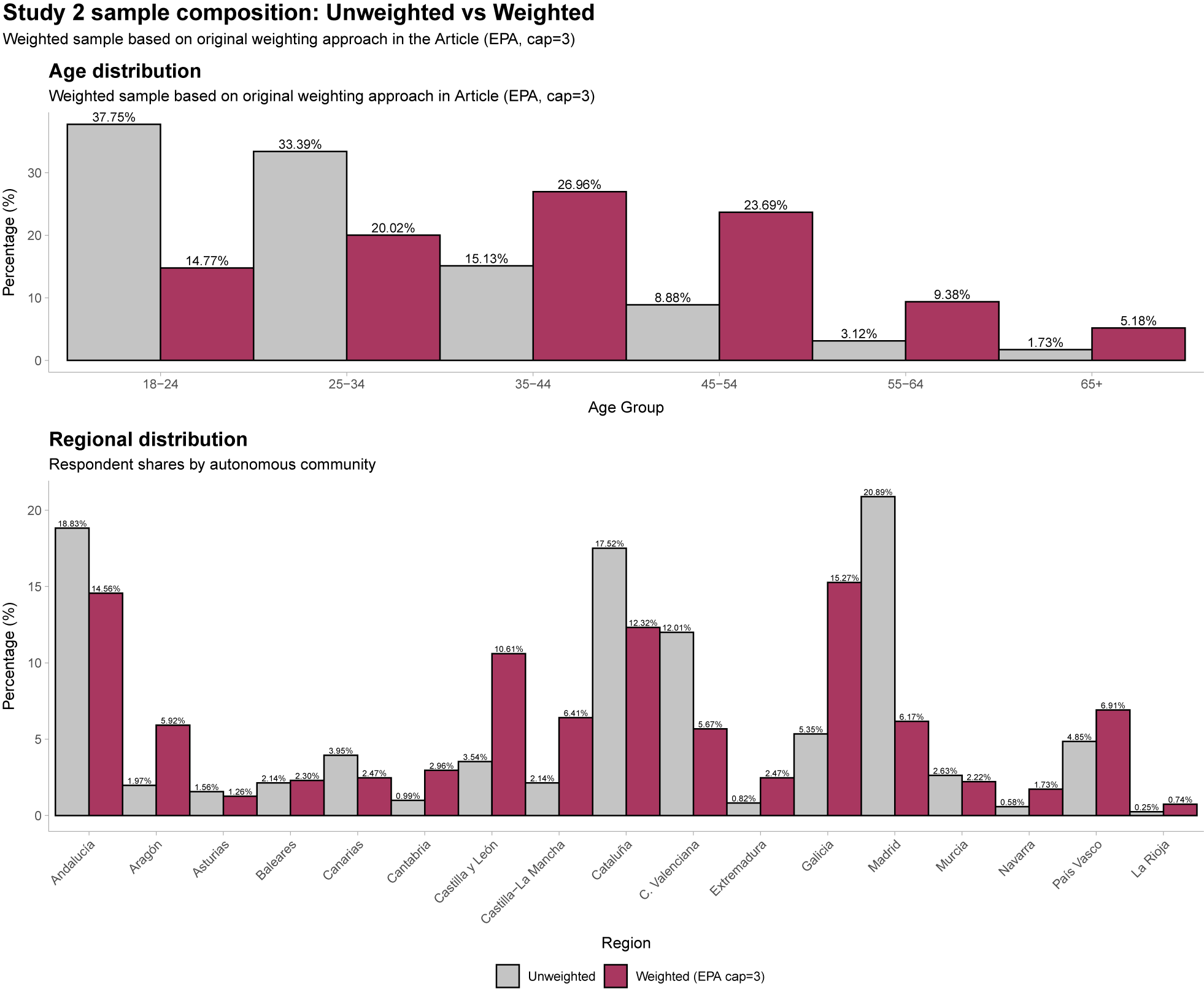
The weighting dispute in the Comment rests on a prior question: what is the appropriate estimand for Study 2? Our theory concerns the political psychology of adults in Spain and, given our expectation of subgroup variation, differences between those with more positive or negative views toward immigration. The target of inference is therefore a population average treatment effect (PATE), not a sample average treatment effect (SATE) that describes only those who happened to take part in our survey. Miratrix et al. (Reference Miratrix, Sekhon, Theodoridis and Campos2018) are explicit that when the goal is PATE estimation, post-stratification weighting of a convenience sample is not merely permissible but methodologically required; unweighted estimates are only equivalent to weighted ones when the sample is already broadly representative of population parameters—a condition that, as Figure 1 makes plain, the sample for Study 2 decisively fails to meet. The Comment’s preferred unweighted analysis recovers a SATE for a sample dominated by young, urban respondents. That is a legitimate quantity, but it is not the one our theory predicts nor the one our Article claims to estimate.

Figure 1.

Demographic Skew in Unweighted Sample and Correction with Weights

Note: Comparison of age and regional distribution in the unweighted crowd-sourced sample from Prolific against the Spanish adult population (EPA 2022 targets) and the post-stratification weighted sample. Full distribution statistics are reported in Table A1 in the Supplementary Material.

Figure 1. Long description

The figure consists of two vertical bar charts. A legend at the bottom indicates grey bars represent Unweighted data and pink bars represent Weighted E P A cap=3 data.

Top Panel: Age distribution. The y-axis is Percentage % from 0 to 30. The x-axis shows Age Group.

* 18-24: Unweighted 37.75% vs Weighted 14.77%.

* 25-34: Unweighted 33.39% vs Weighted 20.02%.

* 35-44: Unweighted 15.13% vs Weighted 26.96%.

* 45-54: Unweighted 8.88% vs Weighted 23.69%.

* 55-64: Unweighted 3.12% vs Weighted 9.38%.

* 65+: Unweighted 1.73% vs Weighted 5.18%.

Bottom Panel: Regional distribution. The y-axis is Percentage % from 0 to 20. The x-axis lists Spanish regions. Significant discrepancies include:

* Andalucía: Unweighted 18.83% vs Weighted 14.56%.

* Cataluña: Unweighted 17.52% vs Weighted 12.32%.

* Madrid: Unweighted 20.89% vs Weighted 15.27%.

* Other regions like Castilla y León, Galicia, and País Vasco show higher weighted percentages compared to unweighted samples.

The Comment suggests that applying post-stratification weights to a convenience sample is, in itself, problematic and generally discouraged. This claim is not supported by a consensus in the methodological literature. Franco et al. (Reference Franco, Malhotra, Simonovits and Zigerell2017) recommend reporting both weighted and unweighted estimates when possible, but at no point do they argue against weighting convenience samples as the Comment claims. As Franco et al. (Reference Franco, Malhotra, Simonovits and Zigerell2017) highlight, it is not uncommon in political science research to apply post-stratification weights to demographically skewed convenience samples where the aim is to approximate population parameters. A quick search among the replication files of recent publications in high-ranking political science journals reveals that post-stratification weighting is commonplace. See, for example, Baisley and Albaugh (Reference Baisley and Albaugh2025), Barari, Lucas, and Munger (Reference Barari, Lucas and Munger2025), Broockman and Kalla (Reference Broockman and Kalla2025), Culpepper, Jung, and Lee (Reference Culpepper, Jung and Lee2024), Grose, Malhotra, and Van Houweling (Reference Grose, Malhotra and Van Houweling2015), Hainmueller and Hopkins (Reference Hainmueller and Hopkins2015), Marsh and Peterson (Reference Marsh and Peterson2026), Matanock and García-Sánchez (Reference Matanock and García-Sánchez2018), Mikkelborg (Reference Mikkelborg2025), Schaeffer, Krakowski, and Olsen (Reference Schaeffer, Krakowski and Olsen2024), and Wittenberg et al. (Reference Wittenberg, Baum, Berinsky, De Benedictis-Kessner and Yamamoto2023) for a non-exhaustive list.

The Comment describes the decision to use weights in Study 2 as “inconsistent with the analysis of Study 1, and this inconsistency is not explained or justified.” This is a mischaracterization: the Article clearly states that Study 1 data are based on a representative sample (Article, 1366) and that Study 2 is based on a crowd-sourced sample that we weight to approximate the population (Article, 1370). This difference reflects different sampling designs that are explicitly detailed in the Article, not an ad hoc choice. Had we been able to finance the recruitment of a representative sample for our replication Study 2, this would have been our preferred approach to replicating Study 1. As that was not the case, we corrected the sub-optimal sample with weights, a standard methodological approach in political science survey experiments (Broockman and Kalla Reference Broockman and Kalla2025; Hainmueller and Hopkins Reference Hainmueller and Hopkins2015; Mikkelborg Reference Mikkelborg2025), and explicitly stated doing so in the Article. Given resource constraints, we relied on a crowd-sourced sample for Study 2 sourced from Prolific. While Prolific can provide representative samples for the United Kingdom and the United States, it does not, currently, do so for other countries. The sample of respondents in Study 2 was severely skewed toward younger individuals and those based in Spain’s capital Madrid. As openly stated in the Article (1370), we applied post-stratification weights to correct for the demographic skew of the data.

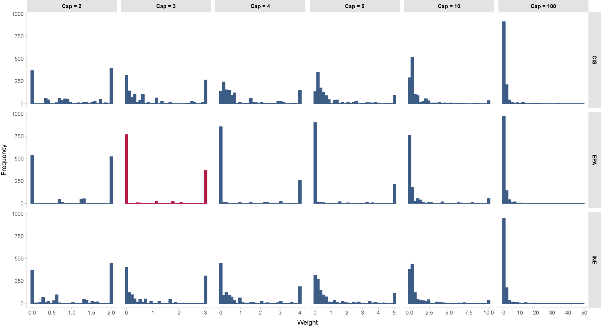
The Comment characterises the bimodal shape of our weight distribution as “peculiar.” In fact, this pattern is a predictable and direct consequence of applying standard weighting procedures to a sample where large subgroups in the raw sample are far from population targets (e.g., under-representation of older respondents and under-representations of regions outside of Madrid) and when weights are capped. In this instance, a bimodal weighting distribution naturally occurs: those over-represented will receive essentially no weight whereas those severely underrepresented will receive the maximum weight. Despite the Comment’s pointed insinuations, and the description of the weight distribution used as “highly unusual,” the Comment made a clear decision not to (i) demonstrate what a usual weighting distribution should look like given the sample and how those used in the Article deviates from it and (ii) create original weights from different population parameters in Spain and compare them to those used in the Article. As we demonstrate in what follows, any simple comparison of the weights used in the Article to a diverse slate of alternative weighting approaches results in comparable results and consistent inferences to those original reported.

Testing the Stability of Results across Alternative Population Weighting Schemes

Given potential concerns about the sensitivity of our findings to population weighting decisions, we conducted a comprehensive robustness analysis using three different Spanish population benchmarks and six different weight capping values. As weighting decisions may represent an additional researcher degree of freedom (Franco et al. Reference Franco, Malhotra, Simonovits and Zigerell2017), our goal here is to verify whether the treatment effects reported in the Article remain stable across multiple alternative weighting approaches and if those reported differ systematically from those that might be observed via the research forking path. They do not: the point estimates reported in the Article are smaller than the median point estimate produced by alternative specifications.

We constructed three separate weighting schemes drawing from authoritative Spanish sources. The first uses the Spanish Labour Force Survey (Encuesta de Población Activa, EPA) from the first quarter of 2022, which provides quarterly employment and demographic data for the Spanish population. This is the weighting procedure applied in the Article. The second employs official population figures from the National Statistics Institute (Instituto Nacional de Estadística, INE) as of July 2022, representing the most authoritative census-based population estimates. The third relies on the Center for Sociological Research (Centro de Investigaciones Sociológicas, CIS) Barometer Survey No. 3366 from June 2022, a major nationally representative political attitudes survey. Each weighting scheme adjusts our sample to match population distributions across gender, six age categories, and Spain’s 17 autonomous communities. Beyond varying population benchmarks, we also tested the sensitivity of results to the weight truncation decision. While our primary analysis employed the default cap of 3 (following standard practice in anesrake), we varied this constraint, testing caps of 2 (most restrictive), 3 (default), and 4, 5, 10, and 100 (effectively uncapped). This yields 18 distinct weight-specification combinations (3 benchmarks × 6 caps), allowing us to assess whether our findings depend on particular weighting choices.

Figure 2 illustrates how weight distributions evolve across these alternative population benchmark sources and weighting caps. The bimodal pattern (with concentrations near 0 and at the cap value, 3) reveals the fundamental challenge of our crowd-sourced sample. Young respondents, who dominate our sample, receive minimal weights (often below 0.01) to down-weight their over representation, while the few older respondents receive maximum weights at the cap threshold. This pattern persists across all three population benchmarks, confirming that the weight distribution is driven by the underlying sample composition rather than the choice of the demographic reference target. As the cap increases from 2 to 100, the distributions become progressively more dispersed. With cap $ =2 $ , weights are tightly constrained between 0 and 2, creating relatively uniform influence across observations but limiting demographic correction. With cap $ =100 $ , the EPA and INE distributions appear nearly identical, while CIS weights show slightly different patterns, particularly in the right tail, reflecting its distinct population profile.

Figure 2.

Distribution of Survey Weights by Reference Scheme and Cap Value

Note: Each panel displays the distribution of survey weights for one of 18 weighting specifications—three population benchmarks (EPA, INE, and CIS) crossed with six weight caps (2, 3, 4, 5, 10, and 100). The bimodal pattern reflects the severe under-representation of certain respondents in the crowd-sourced sample. The highlight panel, EPA at Cap=3 indicates that used in the Article.

Figure 2. Long description

The grid consists of three rows and six columns. The y-axis for all panels represents Frequency from 0 to 1000. The x-axis represents Weight, with scales varying by column based on the cap value.

* Row 1 (C I S): Shows a bimodal distribution at Cap equals 2, which gradually shifts toward a single dominant peak at the lower bound as the cap increases to 100.

* Row 2 (E P A): Displays similar bimodal patterns. The second panel (Cap equals 3) is highlighted in red, showing a high frequency peak near 0 and a secondary peak at 3. As the cap increases to 100, the distribution becomes heavily skewed toward 0.

* Row 3 (I N E): Follows the same trend as the previous rows, with the most extreme right-skewness appearing at Cap equals 100.

Across all panels, the bimodal pattern is most pronounced at lower caps (2, 3, and 4), where significant frequency counts appear at both the minimum and maximum weight values. At higher caps (10, 100), the data concentrates almost entirely at the lower end of the weight scale.

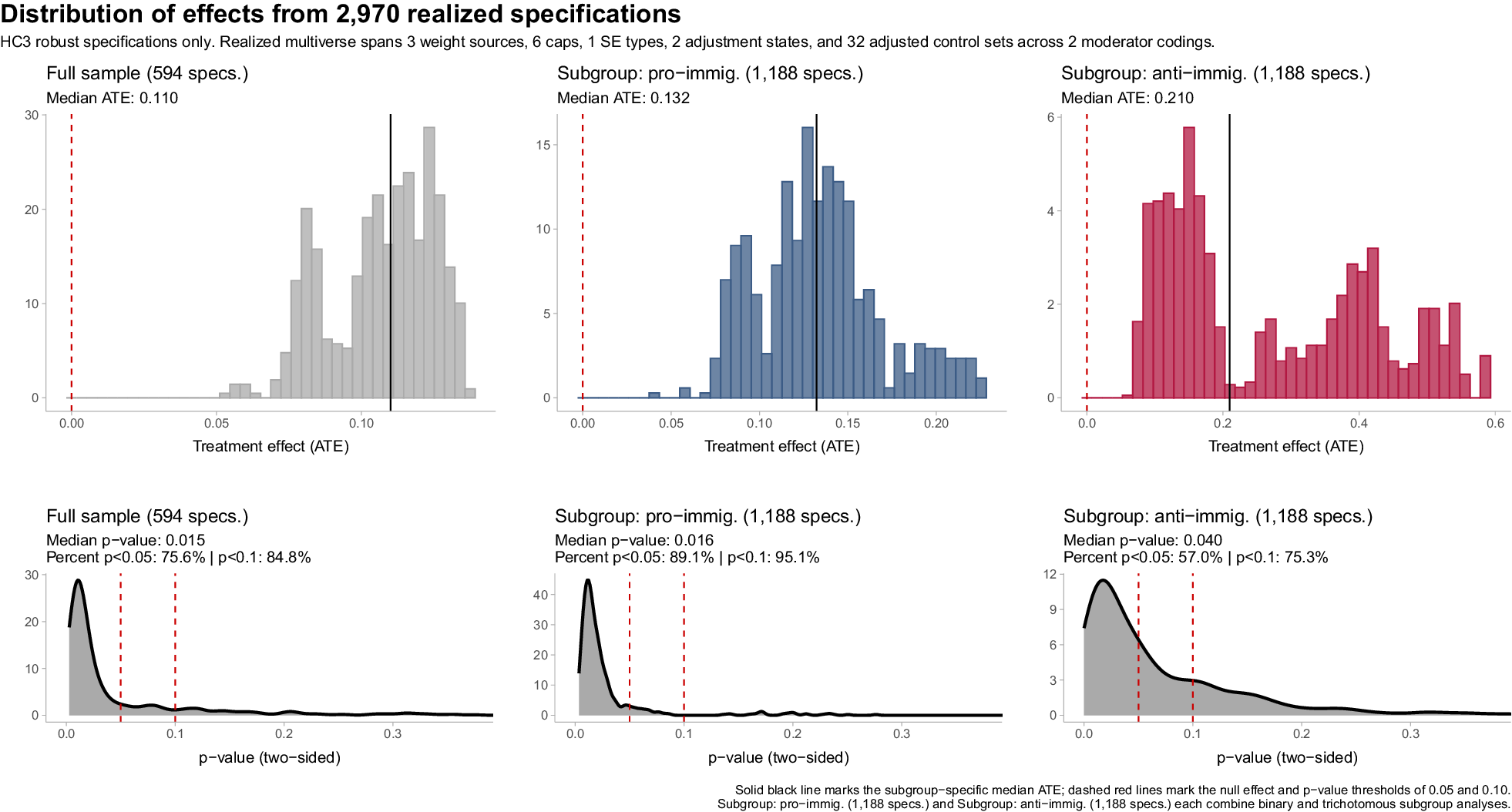
In Figure 3, we demonstrate that treatment effects are stable across weighting alternatives (see also Appendices A.1 and A.3 of the Supplementary Material). Figure 3 reports treatment effects, with robust (HC3) standard errors, that vary the 18 different weighting approaches alongside diverse means of covariate adjustment.Footnote ² The Comment’s primary concern is that the conclusions depend on “ad hoc” weighting choices. We empirically refute this: any sensible approach to demographic adjustment yields consistent conclusions about the instrumental nature of LGBT+ support in response to out-group cues. Our weighting procedure, regardless of its specific implementation, corrects this bias and approximates the treatment effect we could anticipate in a demographically balanced sample. It is also worth highlighting that the distributional position of the Article’s estimates are inconsistent with Comment’s charge of selective analysis. Cherry-picking, the deliberate choice of specifications that favor one’s preferred conclusion, would predict that the reported estimates sit at the upper tail of the distribution of plausible alternatives. The opposite is true. As Figure 3 shows, the originally reported point estimates belong to the lower end of the distribution of estimates generated by the 2,970 alternative specifications. The Article’s estimates are, if anything, conservative relative to the space of defensible analytical choices.

Figure 3.

Treatment Effects and p-Values from 2,970 Alternative Means of Testing the Hypotheses

Note: Summary of 2,970 specifications testing the treatment effect in Study 2 across the full sample and subgroups stratified by pretreatment immigration attitudes (both dichotomous and trichotomous), varying weights applied and covariate adjustment. Each point represents one specification.

Figure 3. Long description

The top row contains three histograms showing the distribution of Treatment effect (A T E). Each plot includes a vertical dashed red line at 0.00 representing the null effect and a solid black line marking the median A T E.

* Top-left: Full sample (594 specs) with a median A T E of 0.110. The data is clustered between 0.05 and 0.15.

* Top-center: Subgroup: pro-immig. (1,188 specs) with a median A T E of 0.132. The distribution is centered around 0.13.

* Top-right: Subgroup: anti-immig. (1,188 specs) with a median A T E of 0.210. The distribution is wider, spanning from 0.1 to 0.6.

The bottom row contains three density plots showing the distribution of p-value (two-sided). Each plot includes vertical dashed red lines at 0.05 and 0.1.

* Bottom-left: Full sample (594 specs). Median p-value: 0.015. Percent p < 0.05: 75.6 percent. Percent p < 0.1: 84.8 percent. The curve peaks sharply near 0.

* Bottom-center: Subgroup: pro-immig. (1,188 specs). Median p-value: 0.016. Percent p < 0.05: 89.1 percent. Percent p < 0.1: 95.1 percent. The curve is highly concentrated near 0.

* Bottom-right: Subgroup: anti-immig. (1,188 specs). Median p-value: 0.040. Percent p < 0.05: 57.0 percent. Percent p < 0.1: 75.3 percent. The curve is broader with a longer tail toward higher p-values.

SECONDARY CONCERNS

In addition to the issue related to the use of weights in a demographically skewed crowd-sourced sample, the Comment raises a number of adjacent concerns. We interpret these concerns as threefold. First, the Comment identifies an incorrect description of the estimations visualized in Figures 3 and 6 in the Article. These figures are erroneously described as being based on an ordinary least squares (OLS) regression. While the corresponding tables referenced within each figure (Article, Tables A7 and A9, respectively) do indeed rely on OLS, the visualizations themselves are based on logistic regression models. This was a coding mistake that likely emerged during revision processes and updating analyses to reflect OLS-versus-logistic regression discussions with reviewers and we regret not updating the figure accordingly to match the tables. Whilst this is obviously an error worth correcting that should not have happened, we also view it as irrelevant to changing the empirical or theoretical conclusions: the error has no bearing on the results and our in-text discussion of the point estimates in the Article reflects those reported in the OLS models.

Second, the Comment identifies that some of the reported coefficients rely on classical standard errors and not robust standard errors. This was a coding error that we did not recognize in the audit of our code.Footnote ³ The Comment correctly identifies some instances where robust standard errors were erroneously not called. This was a mistake and one that could have been avoided had we relied on the estimatr package (Blair et al. Reference Blair, Cooper, Coppock, Humphreys and Sonnet2025) and the corresponding lm_robust function as standard.

We disagree with the Comment, however, when it comes to whether this mistake influences the findings. Our original interpretation of the results from Study 2 in the Article was that treatment induced a positive effect on the outcome (scaled 0–1) among both pro-immigration respondents (CATE $ =0.112 $ ) and anti-immigration respondents (CATE $ =0.102 $ ) but there was no significant difference between the two when the sample was stratified dichotomously. In other words, the effect of treatment was statistically symmetrical for both subgroups (Gelman and Stern Reference Gelman and Stern2006).Footnote ⁴ Based on a trichotomous split, we observed significantly larger effects for the most anti-immigration respondents (CATE $ =0.32 $ ) compared to the most pro-immigration respondents (CATE $ =0.11 $ ). 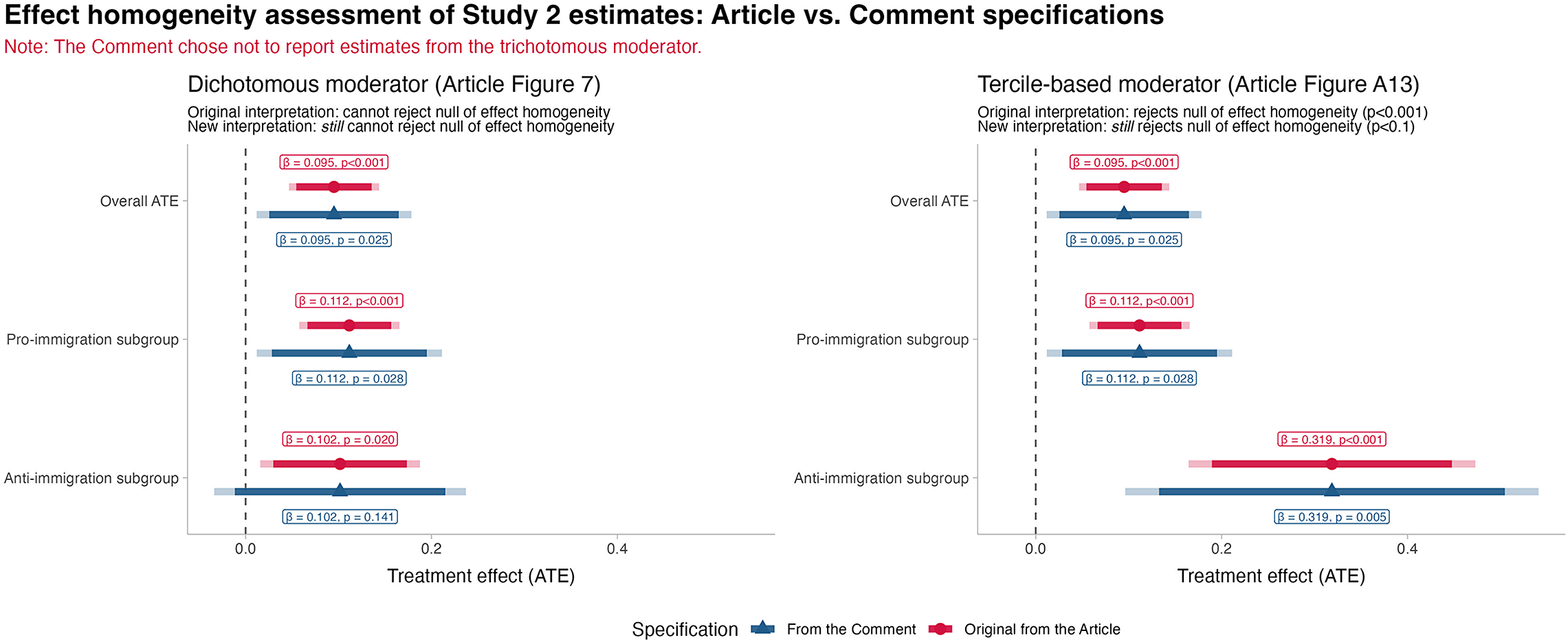The Comment’s claim that “in none of the alternative specifications is the interaction term between treatment and anti-immigration sentiment statistically significant, despite this being the authors’ key theoretical prediction” is flawed. Not only does it mischaracterize our own conclusion of Study 2 as showing no consistent evidence of effect homogeneity (i.e., we transparently stated that the evidence went against our expectations in the original Article), it also actively ignores instances where estimations did observe significant heterogeneous effects. Our interpretation remains the same regardless of standard error choice as we demonstrate in Figure 4.

Figure 4.

Comparing Article and Comment Estimates

Note: Point estimates with 95% and 90% confidence intervals. Original weighting scheme applied. Article: Classical OLS SE. Comment: HC3 robust SE. Null hypothesis of effect homogeneity: CATE (Anti) = CATE (Pro).

Figure 4. Long description

A two-panel forest plot comparing statistical estimates. The x-axis for both panels represents Treatment effect A T E ranging from 0.0 to 0.6. A vertical dashed line marks the zero point. Red markers represent the Original from the Article using Classical O L S S E, while blue markers represent estimates From the Comment using H C 3 robust S E. Each point includes 95% and 90% confidence intervals.

Left Panel: Dichotomous moderator.

- Overall A T E: Both red and blue markers align at beta = 0.095.

- Pro-immigration subgroup: Both markers align at beta = 0.112.

- Anti-immigration subgroup: Both markers align at beta = 0.102.

The interpretation notes that both original and new interpretations cannot reject the null of effect homogeneity.

Right Panel: Tercile-based moderator.

- Overall A T E: Both markers align at beta = 0.095.

- Pro-immigration subgroup: Both markers align at beta = 0.112.

- Anti-immigration subgroup: Both markers align at beta = 0.319, showing a significant shift to the right compared to the left panel.

The interpretation notes that the original rejected the null p < 0.001, while the new interpretation still rejects the null p < 0.1.

Correcting for robust standard errors (the appropriate variance estimator) does not influence the magnitude of our identified effects for each group, nor the difference between the two, across alternative means of stratification. The Comment interprets the reduced significance for the anti-immigration group using the dichotomous stratification as indicative of evidence against our theory. We do not, however, interpret the point estimate of 0.102 for the dichotomous anti-immigration group (representing a 21% increase relative to the control group baseline) on a 0–1 scale as having no effect. P-values on either side of the selected significance threshold allow us to make a claim about whether an effect is statistically distinguishable from zero, but do not indicate that the effect itself is null (Altman and Bland Reference Altman and Martin Bland1995; Rainey Reference Rainey2014). The 0.102 point estimate remains statistically symmetrical to that observed among the full sample, and the dichotomous pro-immigration subgroup. In other words, the effect of treatment for the dichotomous anti-immigration subgroup is qualitatively and statistically symmetrical to that of the dichotomous pro-immigration subgroup even if the former may be, under some specifications, indistinguishable from zero (Gelman and Stern Reference Gelman and Stern2006). The point-estimate from all three models—full sample, anti-immigration, and pro-immigration—are also of a sizeable magnitude that is very unlikely to be observed under the null and the effect among the most anti-immigration tercile subgroup is even stronger at 0.32 ( $ p<0.001 $ ).

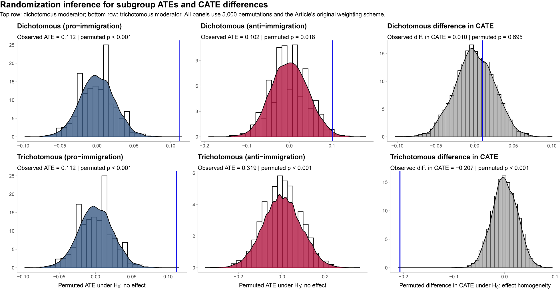
In Figure 5, we empirically demonstrate that the observed point estimate for the dichotomized anti-immigration subgroup, rather than being an effect of zero, is a statistically improbable effect under the null of no effect. Using the ritest package (McDermott Reference McDermott2022), we conducted randomization inference to assess the probability of obtaining the observed point estimates under the null of no treatment effect. For each model (full sample and each subgroup in Study 2), we generated 5,000 permutations of the treatment assignment and re-estimated the effect to form an empirical null distribution. The resulting permutation p-values indicate that the observed effects are statistically rare under the null. For the anti-immigration subgroup (the subgroup analysis where the Comment is concerned with a null effect), the permutation p-value was $ 0.018 $ , meaning that in fewer than 1.8% of shuffled datasets did the effect size meet or exceed the observed value in absolute terms. The permuted 95% confidence interval for this p-value ranged from 0.0145 to 0.022, reinforcing that the result remains unlikely to arise from chance even when accounting for simulation uncertainty.Footnote ⁵

Figure 5.

Comparing the Identified CATE Distribution under (i) the Null of No Effect and (ii) the Null of Effect of Homogeneity

Note: Recall that the Comment chose not to report the results of the tercile-based heterogeneity tests. ATE panels show permutation distributions for subgroup treatment effects. Vertical reference line indicates identified estimate. Table output in Appendix B1 of the Supplementary Material.

Figure 5. Long description

A multi-panel figure with two rows and three columns. The top row represents a dichotomous moderator and the bottom row represents a trichotomous moderator. All panels display a histogram of permuted values with an overlaid density curve and a vertical blue line representing the observed estimate.

Top Row (Dichotomous):

* Left: Dichotomous pro-immigration. Blue distribution centered at 0. Observed A T E equals 0.112, permuted p is less than 0.001. The blue line is far to the right of the distribution.

* Middle: Dichotomous anti-immigration. Red distribution centered at 0. Observed A T E equals 0.102, permuted p equals 0.018. The blue line is on the right tail of the distribution.

* Right: Dichotomous difference in C A T E. Grey distribution centered at 0. Observed diff. in C A T E equals 0.010, permuted p equals 0.695. The blue line is near the center of the distribution.

Bottom Row (Trichotomous):

* Left: Trichotomous pro-immigration. Blue distribution centered at 0. Observed A T E equals 0.112, permuted p is less than 0.001. The blue line is far to the right.

* Middle: Trichotomous anti-immigration. Red distribution centered at 0. Observed A T E equals 0.319, permuted p is less than 0.001. The blue line is far to the right, outside the visible distribution range.

* Right: Trichotomous difference in C A T E. Grey distribution centered at 0. Observed diff. in C A T E equals minus 0.207, permuted p is less than 0.001. The blue line is far to the left of the distribution.

The x-axes for the first two columns are labeled Permuted A T E under H sub 0 no effect. The x-axis for the third column is labeled Permuted difference in C A T E under H sub 0 effect homogeneity.

As shown in Appendix B of the Supplementary Material, where we consider the trichotomous operationalization of the moderator reported in the Article (Figure A13) but absent in the Comment’s reanalysis, permutations reveal that the probability of observing the identified effect under the null is less than 1 in 5,000 (permutation p-value of 0.0002). The Comment’s empirical contribution is that, under some specifications, the identified point estimate is not distinguishable from zero at conventional thresholds. We would highlight, however, that the robustness and sensitivity analyses reported in the Article’s original supplementary material, including multiverse specification curves, also transparently indicated instances where this was the case (see Article, Appendix G).Footnote ⁶ The claim made in the Comment that the inferences made are sensitive to ad hoc selection of standard errors is not supported by the data.

Third and finally, the Comment expresses some taste-based concerns related to the data visualizations. Specifically, the Comment does not agree with the choice not to report confidence intervals for the predicted outcomes even when the average marginal effects are reported with confidence intervals; and the Comment disagrees with the overlaid jittered plot of predicted outcomes and instead would have preferred to observe the overlaid underlying data. These are reasonable stylistic preferences but they are, ultimately, preferences rather than errors and at no point do our visualizations incorrectly label what is displayed beyond the logistic-versus-OLS error already acknowledged. In all figures, estimand uncertainty is reported, and readers are directly pointed toward the corresponding table where standard errors, and p-values are reported. The in-text description of point estimates also explicitly refers to statistical significance where appropriate.