2. RETINA

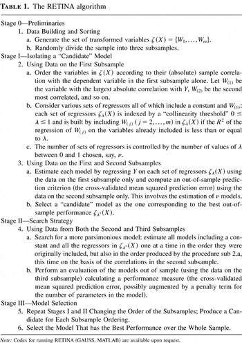
The rationale behind the RETINA procedure is a predictive modeling effort guided by the data structure. In general there is no theory required apart from some guidance in selecting an information set of potential predictive usefulness. The key principles that have inspired the construction of the algorithm are flexibility, selective search, control of collinearity, and out-of-sample predictive ability. The procedure is described in detail in Table 1 (cf. also the original paper by Perez-Amaral, Gallo, and White, 2003); here it is helpful to sketch the motivations for these basic features of RETINA.

The RETINA algorithm

Flexibility: Flexibility is required to handle the lack of information about the functional form of the conditional mean of the dependent variable Y given “inputs” X that is common in economics. To attain this flexibility, one may use a set of transformations of the input variables, say, ζ(X) = {ζ_j(X), j = 1,…,m}, that embodies both nonlinearities and interactions.

Selective Search: The task of evaluating all 2^m possible models arising when we have m candidate regressors in the set of transformed variables ζ(X) and then of applying some form of model selection becomes impossible for even a moderate value of m. Rather, following the ideas in White (1998), we can select from a judiciously chosen subset of all possible models (of order proportional to m), admitting (transformed) predictor variables on the basis of their relevance for the problem at hand. For example, one may rank the candidate regressors according to their correlation in absolute value with the dependent variable and include them in the model sequentially in rank order.

Collinearity: To control the degree of dependency among the variables of the model, one can require that the amount of collinearity between the included predictors and any candidate predictor considered for sequential inclusion must lie below a threshold parameter λ chosen by the experimenter (as λ approaches 0 new regressors approach orthogonality; as λ approaches 1 new regressors may be highly collinear).

Out-of-Sample Forecasting Ability: Although flexibility is desirable, it creates the danger of overfitting the sample data. To avoid this, we use disjoint subsamples for estimation and cross-validation and an out-of-sample prediction performance criterion for model selection as important features of the procedure.

Some comments on the RETINA algorithm are in order.

• Division of the entire sample into three subsamples. This is done to cross-validate using truly out-of-sample data.
• Safeguards against spurious correlations. This is achieved by three features of RETINA. One is the scrambling of the regressors by their correlation in the second subsample, another is the use of the parameter λ to control for collinearity, and a third is the repetition of the whole procedure on the different orderings of the sample.
• Information criteria. To select the final model associated with a specific ordering of the subsamples we apply an information criterion; RETINA uses the out-of-sample Akaike information criterion (AIC).

3. PcGets VERSUS RETINA

In this section we sketch similarities and differences between PcGets and RETINA. For clarity and brevity, we omit details that can be found in the references. We start by comparing the objectives, strategies, and general characteristics of the two procedures, continue with some more specific details, and finally outline certain parallel aspects of the two methods.

In many practical applications, the general-to-specific approach often proceeds as if the DGP is nested within the GUM (or, equivalently, as if the GUM is an overparameterization of the DGP), so that the DGP can be discovered by eliminating the irrelevant variables (this is not an explicit assumption of PcGets, though). RETINA is less ambitious. It tries to approximate an unknown predictive relationship using a model that is not necessarily correctly specified, using transforms of the attributes to the extent that they contribute to out-of-sample prediction and are not too collinear with each other.

The modeling strategies are quite different: PcGets proceeds from general to specific; it starts from a general model and reduces it. RETINA starts from a model with just a constant and augments it by including additional transforms only when they help forecast out of sample and are not too collinear with previously included variables (no specific hypothesis testing is performed).

The role of the GUM is crucial in PcGets, but there is no automatic procedure for specifying the GUM, although there are useful guidelines. On the other hand, RETINA constructs several base models (GUMs in PcGets parlance) in an automatic fashion and then uses a strategy to reduce them using out-of-sample performance criteria.

A priority within the RETINA procedure is the control of collinearity among the variables as represented in the initial information set and after subsequent nonlinear transformations. (Note that linear transformations are excluded from consideration as candidate regressors.) Collinearity is not as central a concern for PcGets, although Hendry often advocates reparameterizations of the GUM so as to strive for orthogonal regressors.

In PcGets two overlapping subsamples are used for postchoice evaluation, but not for model selection. They are used to check for in-sample goodness of fit. However, the model building and selection mechanism of RETINA is directed toward out-of-sample predictive ability. That is why it is necessary to use disjoint subsamples for performing out-of-sample forecasts and carrying out truly out-of-sample forecast evaluations.

The linearity or nonlinearity in the underlying variables afforded by PcGets is specified by the GUM. The nonlinearity in the underlying variables of the model selected by RETINA is chosen by the procedure. Linearity in the parameters ensures simple computation.

The functional form of the model suggested by PcGets is embedded in the GUM. The functional form of the model suggested by RETINA is given by the original inputs and the transforms allowed by the procedure.

Undoubtedly, the two procedures have certain parallel features. Both apply repeated testing: PcGets reduces the GUM from the top down with in-sample tests, whereas RETINA builds from the bottom up by adding regressors one by one, in the order suggested by a saliency feature, controlling for collinearity, and then repeatedly using out-of-sample tests and an information criterion, the out-of-sample AIC, for trimming the model down.

Despite these parallel features, especially in the mechanics, PcGets and RETINA are nevertheless distinct in terms of objectives, general strategy, selection criterion, the base model, flexibility of the model, treatment of collinearity, and the use of the subsamples.

The procedures can be seen as different but far from incompatible ways of providing insights into a set of data. Different emphases are at work, and, in particular applications, one may be more useful than the other, depending on prior knowledge, the intended use of the model, and the ability of the researcher.

4. RETINA AND PcGets: AN APPLICATION

The aim of this section is to illustrate the performance of RETINA and PcGets using a real data set. The comparison is necessarily limited in scope, because the GUM is crucial for PcGets, and its specification is crucial for a proper comparison with other methods. We do not have clear indications as to what might be legitimate GUMs in our particular application, so we use simple models to start with and feed the same inputs to the linear regression model, RETINA and PcGets. By the same token, not having strong hypotheses about the function linking the available information is a fundamental basis for the use of RETINA.

For our application we use a cross-section of U.S. firms. The data were obtained from PNR, a subsidiary of Indetec International. The data set includes variables related to the demand for business toll telephone services in 1997. Our main interest is the duration of “intra-lata” calls. (LATA stands for “local access and transport area.”) A toll call from one point within a LATA to another point within the same LATA is an intra-lata or short distance toll call. Possible explanatory variables of intra-lata duration are business lines (Bus), the number of hunting lines (Hun), the sales (Sales) of the company expressed in dollars, the number of employees working locally (Emh), the total number of employees for the business (Emt), the physical extension of the business, proxied by the square footage of its premises (Sqft), and population (Pop), that is, the size of the business area location.

Our sample has 1,217 observations. Prior to the analysis, the data were rescaled to avoid the eventual negative impact on computations of large differences in orders of magnitudes of the variables. Given our purposes here, we focus on the performance of RETINA with respect to the more traditional use of a linear model. We do not consider prior transformations of the original variables, although a log transform of the dependent variable or its ratio by the number of employees (which is common in the Telecom demand literature) could also be considered (which also raises the issue of what transformation for the dependent variable should be considered). We model intra-lata minutes as a function of the number of business lines, the number of hunting lines, employees here, employees total, sales, square footage, and population habitat size.

To evaluate the candidate models, we use two criteria. The first is based on an information criterion; specifically, we choose the model with the lowest AIC. The second is the out-of-sample performance, measured by cross-validated mean square prediction error (CMSPE), which we expect to be lower for models suggested by RETINA. To compute a consistent measure of CMSPE, we used the following strategy, motivated by the fact that CMSPE depends on the specific subsample split considered, in terms of its size and characteristics.

We randomly assigned each observation to three disjoint subsamples, each including approximately one-third of the observations in the sample. Then the proposed models were cross-validated using two of the three subsamples for estimation and the third for cross-validation. We considered all three possible rotations and then summed the CMSPEs obtained in each rotation.

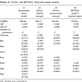
In Table 2, we compare several model estimations. In column 1, we report the estimation of a usual linear model (by ordinary least squares [OLS]) without using an automatic model selection strategy. The signs of the coefficients are as expected, except for Sales and Population, which are not statistically significant. The results suggest that the number of business lines (Bus), labor force (Emh, Emt), and physical extension of the business (Sqft) should be important for explaining the duration of intra-lata calls.

PcGets and RETINA: Selected simple models

In columns 2 and 3 we report the results of PcGets taking the standard linear model as the GUM. The liberal strategy drops the two insignificant variables of the basic linear model and obtains a slightly lower AIC and a better CMSPE, providing an improvement over the basic model. The conservative strategy drops an additional variable, hunting lines [Hun], with a slight increase in AIC and worsening of the CMSPE. In terms of prediction, it is still better than the basic model of column 1.

In column 4, we report the model suggested by RETINA without allowing any transformation of the inputs. We do this to obtain a direct comparison with the basic linear model and with the models suggested by PcGets. We observe that the first model suggested by RETINA, model 1, is very similar to the conservative PcGets model. The difference is that it substitutes [Hun] for [Emt].

The comparison of columns 2 and 4 illustrates how RETINA has improved out-of-sample predictive ability (corresponding to an improvement of the CMSPE from 896.11 to 770.86) by dropping the variable Emt even if it is highly significant in sample, with a t-statistic of 5.07, a result that parallels the outcomes in the simpler models seen in Table 2. If one had a strong prior on the theoretical relevance of such a variable, the indications provided by the automated procedure should definitely be taken into account.

In this case, RETINA chooses just one of the two variables related to Employees in the model, as the number of workers locally and in the whole business is highly correlated (Pearson's correlation = 0.86). On the other hand, it excludes more descriptive and nonsignificant variables such as Sales and Population.

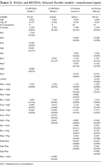
A distinguishing feature of RETINA is its use of nonlinear and interactive transforms of the underlying predictors. Accordingly, in Table 3—columns 1 and 2—we report the results obtained by RETINA, permitting it the use of nonlinear transforms and interactions created by taking all squares, cross-products, and cross-ratios. For brevity, we do not explicitly reference all such ratios as most of these are never selected. As a result the out-of-sample (and also the in-sample) performance improves significantly relative to the results of Table 2, while at the same time being only slightly less parsimonious than the simple linear model of Table 2. RETINA model 2 (column 1) was chosen using a minimum AIC criterion and RETINA model 3 (column 2) considering the minimum CMSPE.

PcGets and RETINA: Selected flexible models—transformed inputs

The total variation explained by these models is noticeably higher than models with the original inputs, whereas the CMPSEs for models 2 and 3 are respectively 37% and 43% lower than that of the first basic model (column 1).

The transformations suggested by RETINA for both models 2 and 3, in particular the interaction terms, are interesting. The negative constant terms in Table 2, columns 1–4, become positive in Table 3, columns 1 and 2, in which RETINA allows for transformed inputs. These models are not necessarily correctly specified, and we emphasize that this implies that the coefficients thus do not necessarily have the standard ceteris paribus interpretation.

Although PcGets is designed to identify a theory-congruent parsimonious model corresponding to the true DGP, it may nevertheless have value in obtaining forecasts. To investigate the properties of PcGets in this regard in a manner directly comparable to our RETINA results, we apply PcGets by specifying a GUM that contains all the transforms accessible to RETINA. Strictly speaking, this is a nonstandard approach to PcGets, as we have no theory justifying this specification of the GUM, nor a guarantee that the result may be theoretically plausible. We may be placing theory congruence at risk, and we make no attempt to specify relatively orthogonal regressors. Nevertheless, we see from columns 3 and 4 of Table 3 that both conservative and liberal versions of PcGets not only provide noticeable improvements in CMSPE and AIC relative to all the models of Table 2 but also improvements relative to the RETINA results of columns 1 and 2 of Table 3 (CMSPE of column 3 of PcGets is 3.7% lower than column 2 of RETINA).

That PcGets is useful in this context should not, however, be surprising, considering that (as is plausibly true here) even when the GUM does not include the DGP (the ideal forecasting tool), PcGets should identify an approximation to the DGP that has certain optimality properties and that may thus be useful in forecasting. Interestingly, although PcGets is designed to deliver parsimonious models, it achieves its modest gains relative to RETINA with models that are twice as complex.

We emphasize the strictly limited scope of the preceding comparison. Nevertheless, our example illustrates that RETINA may help the researcher not only to arrive at useful forecasting models but also to consider relevant transformations of the inputs that, when used as regressors, yield models with improved forecasting ability relative to the basic regression model. Further, we see that PcGets has value in obtaining useful forecasts. It is an interesting question to investigate whether the use of PcGets for this purpose generically results in less parsimonious models than RETINA or whether this is only a feature of our present example.