1. Introduction
While economic growth in developing countries is a desirable goal, its side effects of rising energy demand and greenhouse gas emissions are problematic in light of global warming. The controversial discussions during the Bali climate policy conference in 2007 showed that including the developing countries in a post-Kyoto agreement in a fair way is a challenge, and it was emphasized that the industrialized countries need to support the developing countries by technical, financial, and educational measures.
One possibility to slow down rising emissions is energy-saving technology transfer to developing countries, since energy use is strongly related to carbon emissions. It is thus important to detect how international technology transfer occurs and how it affects energy supply and demand. Foreign direct investment (FDI) is regarded as one important channel for technology transfer in general (e.g., Keller, Reference Keller2004). Empirical evidence on energy-saving international technology transfer could answer the question whether more FDI flows to developing countries can effectively help to restrain energy use and thus greenhouse gas emissions. In this paper we use a large macro-level panel dataset and investigate empirically whether FDI inflows have a significant effect on energy intensities of developing countries.
Despite the relevance of the topic, little empirical evidence exists regarding the transfer of energy-saving technologies. Some case studies and microeconometric work using firm-level data indicate that foreign-owned firms in specific developing countries indeed use less energy than their indigenous counterparts (Eskeland and Harrison, Reference Eskeland and Harrison2003; Fisher-Vanden et al., Reference Fisher-Vanden, Jefferson, Liu and Tao2004). However, comprehensive studies on an aggregate level with cross-country data are missing. This is unfortunate, since they can potentially give a broader picture of the issue at hand and can answer the question whether the findings from specific plant-level studies can be generalized on a global scale. The question of generalization is important in light of recent worldwide initiatives to reduce energy use and emissions. Mielnik and Goldemberg (Reference Mielnik and Goldemberg2002) have used data from 20 developing countries and found a negative effect of FDI on energy intensity. However, this analysis controls for no other influences on energy intensity and does not take the unit root behavior of the variables into account. Hence, rather than providing general evidence, the results by Mielnik and Goldemberg (Reference Mielnik and Goldemberg2002) open a promising way for further research.
In this paper we use a large macro-level panel dataset and an extended econometric model in order to broaden the analysis and to investigate whether FDI has a general impact on energy intensity. The dataset includes 60 developing countries for the years 1975–2004. In contrast to the hypothesis proposed by Mielnik and Goldemberg (Reference Mielnik and Goldemberg2002), we find no robust energy-reducing effect of FDI inflows in developing countries. The interactions of FDI inflows with country-specific characteristics yield no significant results, either. For policy makers who seek to achieve energy reductions in developing countries, our results imply that a general support of FDI inflows is not enough; it is rather necessary to explicitly encourage the kind of FDI that brings about energy-reducing technology transfer. Issue linkage, as for example the clean development mechanism in the Kyoto Protocol, might be a way to achieve this objective.
Our paper is structured as follows: Section 2 explains the theoretical background and reviews related empirical evidence in the literature. We furthermore replicate a simplified regression analysis as in Mielnik and Goldemberg (Reference Mielnik and Goldemberg2002) and show why an extended empirical approach is needed to generate meaningful results. In section 3, we first derive our empirical model based on the insights from the theoretical considerations. We then specify our estimating equations, apply regression analyses, and discuss the results. Section 4 presents our robustness checks using a modified database. Section 5 concludes.
2. The influence of FDI inflows on energy use
In this section we first present the conceptual background for the hypothesis that FDI has an energy-reducing effect in the destination country. Then we give an overview of the empirical literature examining the evidence on energy-reducing technology transfer via FDI and discuss in more detail the analysis by Mielnik and Goldemberg (Reference Mielnik and Goldemberg2002).
2.1. Theoretical background
In the literature on trade and the environment, it has become common to decompose the effects of economic activity and trade on pollution into a scale, a composition, and a technique effect. This decomposition was introduced by Grossman and Krueger (Reference Grossman, Krueger and Garber1993), who examined data on concentrations of sulfur dioxide and suspended particulate matter. It was later on backed up with formal theory by Antweiler et al. (Reference Antweiler, Copeland and Taylor2001) and further elaborated by Copeland and Taylor (Reference Copeland and Taylor2003). As argued by Cole (Reference Cole2006), the framework from the trade and environment literature is also applicable to energy use, since energy use is the principal cause of most air pollutants. In our analysis, we adapt the concept developed by Antweiler et al. (Reference Antweiler, Copeland and Taylor2001) and examine how scale, composition, and technique effects influence total energy use.
For simplicity, we split up total economic activity into two sectors with different energy intensities: industry and non-industry. Energy use in the non-industry sector relative to its output value is defined by e(A) with the properties e(A) > 0 and e’(A) < 0, where A is a proxy for the average technology in use. We assume that the energy intensity in the industry sector is always μ times higher than e(A). Measuring total output by gross domestic product (GDP) and denoting the share of industrial value added in output by IND, total energy use can be written as

It follows from (1) that total energy use in a country can be decomposed into three factors: the scale of overall economic activity (GDP), the relative importance of energy-intensive sectors in economic activity (IND), and the energy intensity of the technology in use (e(A)). In analogy to Antweiler et al. (Reference Antweiler, Copeland and Taylor2001), changes in these factors can be interpreted in the following way: The first term is obviously the scale effect and reflects the impact of increasing or decreasing economic activity on total energy use when holding constant the mix of sectors as well as the technology. The second term is the composition effect; holding scale and technology constant and producing relatively more energy-intensive goods due to a sectoral shift leads to an increase in energy use. The last term captures the technique effect resulting from the implementation of a more energy-efficient technology A that reduces the input of energy into the production process.
Having set out the fundamental factors affecting energy use, we can now identify the variables that influence these factors. In this context, we pay special attention to the effects of FDI inflows.
The scale effect can be directly measured by changes in the observable variable GDP. For constant returns to scale of production functions, an output increase leads to a proportional increase in energy inputs. This means that energy intensity, defined as energy use divided by GDP, remains constant.Footnote 1 FDI can influence the scale effect indirectly: since FDI inflows are assumed to stimulate economic growth and since expanded economic activity is related to higher energy use, the scale effect resulting from FDI inflows is positive, and its extent depends on the magnitude of the influence of FDI on GDP.
Changes in the relative importance of the production of energy-intensive goods, i.e., the composition effect, are determined by changes in the sectoral structure of an economy. A typical empirical observation is that in the early stages of a country's economic development, economic activity shifts from the agricultural to the industrial sector. Since the latter is more energy intensive than the former, this implies a positive composition effect. Later in the development process, activity moves typically from the industry to the service sector or from the heavy to the lighter industry. This implies a negative composition effect in this stage, as the service sector and the light industry are less energy intensive (Stern, Reference Stern2004). One reason for such a development pattern can be changes in the comparative advantage of an open economy in the world market. The comparative advantage can be influenced by variables like the capital-to-labor ratio, environmental regulations, or the share of skilled labor. FDI inflows contribute to the composition effect if they change the sectoral structure of an economy. In equation (1) we measure sectoral shifts directly by changes in the share of industrial value added in GDP. This means that all the indirect influences on the sectoral structure, including the composition effect of FDI, are already captured by the inclusion of this variable.
The technique effect covers the impact of employing new technologies or management practices on energy use. We hypothesize that novel technologies developed with a higher level of knowledge are more productive and hence more energy efficient than old technologies. In analogy to Arrow (Reference Arrow1962), we propose that learning is a function of cumulated gross investment, which we denote by GI .Footnote 2 This means that accumulated knowledge increases with every new capital good being available. The hypothesis brought forward by Mielnik and Goldemberg (Reference Mielnik and Goldemberg2002) is that imported investments via FDI in developing countries have a stronger energy-reducing effect than new domestic investments. This can be the case through technology transfer via FDI so that developing countries are able to ‘leapfrog’ over traditional technologies in use. In order to test this hypothesis, we explicitly consider the accumulated FDI inflows G FDI as a determinant of energy intensity, which represents a source of accumulated knowledge that might differ from accumulated domestic investment in its strength. We furthermore add the accumulated import value G IM and the accumulated foreign aid value G AID as further potential sources of technology transfer. All three variables are expressed as shares relative to overall cumulative gross investment GI , since the shares of foreign capital (embodied in FDI, imports, or aid) in total capital represent the relative importance of transferred knowledge in the economy (similar to Aitken and Harrison, Reference Aitken and Harrison1999). A different driver of the energy-saving technique effect can be income per capita, which can be explained by a political economy mechanism: Since environmental quality is assumed to be a normal good, rising per-capita income leads to higher public appreciation of a clean environment. The rising demand for environmental quality may then result in the adoption of stricter environmental regulation that typically also provides incentives to reduce energy use.Footnote 3 Firms react to the regulation by the introduction of cleaner and more energy-efficient technologies. This effect, which is related to the so-called environmental Kuznets curve (EKC), is in the following referred to as income-induced technique effect.Footnote 4 Summing up, we expect that the energy intensity of a country's technology, e(A), depends negatively on accumulated gross investment, GI , and might be reduced further by the extent of the respective shares of accumulated FDI, imports and aid in accumulated investment. Furthermore, the income level per capita (YPC) might reduce energy intensity so that e(A) is a function of

With regard to FDI, it is also possible to establish an indirect link to the income-induced technique effect, namely, under the assumption that openness to trade and FDI enhances growth and hence per-capita income. Grossman and Krueger (Reference Grossman, Krueger and Garber1993) emphasized especially this indirect effect when they analyzed the technique effect of trade liberalization. In the theoretical model by Antweiler et al. (Reference Antweiler, Copeland and Taylor2001), the income-induced technique effect is the only technique effect resulting from increasing openness.Footnote 5 While the literature on trade and the environment has mainly focused on the income-induced technique effect, the broader literature on technological change has recently expanded with numerous studies on technology transfer resulting from openness to trade and FDI (for an overview, see Keller, Reference Keller2004). Technology transfer via FDI, which potentially also reduces energy use, can occur in two ways: first, directly via more efficient foreign firms operating in the host country and, second, indirectly through technological spillovers from foreign firms to indigenous firms. For these mechanisms to be effective, we make the assumption that the technology used by foreign investors is typically superior to the technology that is currently in place in developing countries. The direct effect implies that the foreign-owned firm, compared to a similar indigenous firm, uses less energy and hence contributes to the technique effect. Regarding the technological spillovers, the literature suggests three potential channels: demonstration effects, which stand for imitation and reverse engineering by local firms; labor turnover, which implies the transfer of knowledge by workers who change their employer; and vertical linkages, which involve that multinationals transfer technology to their suppliers or customers (Saggi, Reference Saggi2002). Additionally, higher exports and imports as well as FDI inflows are likely lead to increased competition. Firms need to become more productive in order to stay competitive in the export market or to compete with imports and new foreign companies in the domestic market. For instance, Corcos et al. (Reference Corcos, Del Gatto, Mion and Ottaviano2007) applied a theoretical model with heterogeneous firms and assumed that international trade increases aggregate productivity through a selection effect: the least productive firms leave the market under increased pressure from competition. One can expect that higher productivity also implies more efficient energy use in production.
Though we identified several indirect influences of FDI inflows on energy use through scale, composition, and technique effects, note that all the indirect effects are implicitly included in the variables GDP (scale effect), IND (composition effect), and YPC (income-induced technique effect). We therefore propose that any remaining direct influence of FDI can be attributed to technology transfer, and the main contribution of our analysis is to identify and quantify this influence empirically.
2.2. Empirical literature on energy-saving technology transfer via FDI
There is a large and growing empirical strand of literature on productivity-improving technology transfer and spillovers through FDI. The evidence is mixed, but Keller (Reference Keller2004: 771) notes in his survey paper that ‘recent micro productivity studies tend to estimate positive, and in some cases also economically large spillovers associated with FDI’.Footnote 6 Among other studies, Tybout (Reference Tybout, Choi and Harrigan2003) found evidence for efficiency improvements due to higher exposure to foreign competition as predicted by the New Trade Theory. However, he pointed out that it is not clear according to the related literature whether international activities cause the improved efficiency or vice versa. Furthermore, none of these empirical studies sheds light on the effects of spillovers and productivity gains on energy efficiency.
In the following, we focus specifically on energy-saving technology transfer via FDI. Peterson (Reference Peterson2008) reviewed the existing evidence and remarked that although there may be a large potential for such technology transfer, there is a lack of knowledge about its empirical magnitude and its drivers, and the topic remains insufficiently researched. The hypothesis that foreign-owned companies use less energy than their indigenous counterparts in developing countries is confirmed by studies based on firm-level data. In their analysis of manufacturing plants in Cote d'Ivoire, Mexico, and Venezuela, Eskeland and Harrison (Reference Eskeland and Harrison2003) found that foreign ownership is associated with less energy use. A similar result has been documented by Fisher-Vanden et al. (Reference Fisher-Vanden, Jefferson, Liu and Tao2004), who found a negative impact of foreign ownership on the energy intensity of Chinese companies. These examples suggest that the more efficient technologies of foreign firms can indeed contribute to an energy-reducing technique effect via technology transfer.
On an aggregate level, only very few studies link openness and FDI to energy-saving technology transfer. Cole (Reference Cole2006) used a variation of the model developed by Antweiler et al. (Reference Antweiler, Copeland and Taylor2001) to examine the impact of trade intensity (while not explicitly including FDI) on energy use in 32 developed and developing countries. His panel estimation yielded that the effect of liberalization is country specific and can be positive or negative, depending on whether the country is importing or exporting the energy-intensive good.
Mielnik and Goldemberg (Reference Mielnik and Goldemberg2002) carried out a simplified regression as a starting point for further research on the basis of previous evidence that developing and industrialized countries are converging to a common pattern of energy use (Mielnik and Goldemberg, Reference Mielnik and Goldemberg2000). Their results indicate that the quantity of FDI inflows has a negative influence on energy intensity. They used a sample of 20 developing countriesFootnote 7 for the years 1987–1998, aggregating all countries to one time series, and estimated the regression:

The dependent variable EI t is energy intensity in year t, i.e., the sum of total energy use in all 20 countries divided by their GDP, which is measured in purchasing-power parity. The explanatory variable FDI t /It represents inflows of FDI as a fraction of total gross investment in all countries; ϵt is the error term.
First, we reproduce the regression by Mielnik and Goldemberg (Reference Mielnik and Goldemberg2002) with the same 20 countries but for an extended time span. Complete data on gross fixed capital formation (gross investment) is available for each of the 20 countries from 1979 to 2003. We evaluate our dataset with the same regression model as Mielnik and Goldemberg (Reference Mielnik and Goldemberg2002) and find a similar result, which supports the view of a strong energy-reducing impact of FDI: FDI t /It has a negative coefficient β 1 equal to −0.774; the constant β 0 is 0.320; and R 2 is 0.818. However, the result of this ordinary least squares (OLS) estimation relies critically on the stationarity assumption of the involved variables.Footnote 8 If at least one variable is instead integrated, which implies non-stationarity, standard OLS regression analysis is not appropriate and can result in a spurious regression (compare Granger and Newbold, Reference Granger and Newbold1974).
We check the variables for the stationarity property via the augmented Dickey–Fuller (ADF) test for unit roots. According to obvious trends in the data, we test both variables against stationarity around a deterministic trend.Footnote 9 The null hypothesis of a unit root cannot be rejected in all tests of the variables in levels but can be rejected in case of first differences. Thus, the variables energy intensity and FDI as a fraction of total investment are both integrated of order one. Furthermore, we employ the Johansen cointegration test. Using the variables EI t and FDI t /It and examining three possible model specifications, no cointegration can be found in any case. The results of the preceding tests show that the estimation results obtained from the classical OLS regression are likely to be misleading, and we need to treat a simplified regression analysis with caution.
3. Panel data analysis
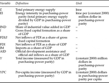
In order to find robust empirical evidence for energy-saving international technology transfer via FDI, we use aggregated country-level data for 60 developing countries in the period 1975–2004. Thereby we refer to all Non-Annex I Parties of the Kyoto Protocol as developing countries. Excluding the countries with insufficient data availability (among them all countries that have emerged from the former Soviet Union) results in our sample of 60 countries.Footnote 10 Data on total primary energy supply are taken from the International Energy Agency (2007). Data on all other variables are found in the World Development Indicators by the World Bank (2007) and, if not available there for specific countries, from the Balance of Payments Statistics and the International Financial Statistics of the International Monetary Fund (2007a, b). An exact definition of the variables and units used in the regressions is presented in table 1.Footnote 11
Definition of variables

In our extended empirical specifications we take potential non-stationarity of the time series into account and use several control variables derived from our theoretical framework. Moreover, we account for the heterogeneity of countries by applying panel data methods. This is recommendable, since the aggregation of all countries would eliminate heterogeneity, which is obviously present in our sample of 60 countries.
3.1. Derivation of the empirical model
We derive our empirical model for energy use from the theoretical framework and the variables presented in section 2.1. Hence, we need to add up the scale effect, the composition effect, and the technique effect. In the case of constant returns to scale, the absolute size of an economy measured by GDP has no influence on energy intensity. We therefore leave the scale effect aside and analyze energy intensity EI as the dependent variable, i.e., total primary energy supply divided by GDP (as in Mielnik and Goldemberg, Reference Mielnik and Goldemberg2002; Cole, Reference Cole2006), where GDP is measured in purchasing-power parities.Footnote 12 Furthermore using a multiplicative form for equation (2), inserting it in (1), and taking logs, the energy intensity of developing country i at time t can be expressed as

We are not able to include all the various influences on energy use, since many of them are determined on the micro level and the necessary micro data is not available for most developing countries. Examples are the detailed sectoral structure of the industry, local economic and environmental regulations, and energy prices. The way in which we will implicitly capture country- or time-specific effects in the estimation is to use panel data models with cross-section fixed effects or random effects and time fixed effects.
We test the available variables for the presence of a stochastic trend and thus on stationarity. We apply several unit root tests for panel data and allow for individual trends and intercepts.Footnote 13 Not surprisingly, we find unit roots for total primary energy supply, GDP, and GDP per capita (as confirmed in other empirical studies, e.g., Perman and Stern, Reference Perman and Stern2003).Footnote 14 Regarding energy intensity (primary energy supply divided by GDP) the unit root hypothesis is rejected. However, the probability of error in this case is close to 5 per cent, which indicates some uncertainties about the properties of this variable. As a consequence of the unit root tests’ results, we transform our estimation model into first differences, where according to the test statistics all variables are stationary without doubt.
Approximating ln (μ · INDit + 1 − INDit) in equation (4) by (μ − 1) · INDit and taking first time differences leads to

Note that Δln can also be expressed by relative changes; for instance, I it/G I it means gross investment flow in year t over cumulative gross investment up to year t. We now assume for reasons of data availability that accumulated flows of investment, FDI, imports, and aid are proportional to the GDP of the respective economy in year t, for example, G FDIit = σ2 Yit. Equation (5) then reads

Writing the coefficients in a more comprehensive way and, for convenience, denoting the shares of investment, FDI, import, and aid flows in GDP by Iit, FDIit, IMit, and AIDit respectively, leads to our empirical model:

Linking the model to our conceptual framework, the coefficients of FDIit, IMit, and AIDit encompass international technology transfer, while the coefficient of Iit also includes a domestic vintage capital effect that may contribute to a reduction of energy intensity. The composition effect is captured by ΔINDit, the change in the share of industrial value added in GDP. The income-induced technique effect, which FDI may also bring about via rising incomes, is accounted for by the relative change in per-capita income ΔlnYPCit. The scale effect is implicitly included, since we examine energy use relative to the size of the economy represented by GDP.
Our hypothesis of energy savings via FDI implies that β 3 is negative. The interpretation is straightforward: FDI inflows in a certain year decrease energy intensity in relative terms, whereas ceteris paribus energy intensity stays constant if there is no FDI inflow. The higher the FDI inflow intensity, the higher the relative reduction of energy intensity. This is consistent with the notion that FDI inflows continuously bring about technology transfer that can reduce energy intensity. The coefficients of imports and aid can be interpreted in the same way.
3.2. The estimating equations
Since there is considerable heterogeneity in the development of energy intensities among countries, we allow for unobserved effects in the estimation. To check the need for country-specific effects we carry out likelihood ratio tests (LR-tests) and F-tests on poolability. (Note that country-specific effects in the differenced equation imply country-specific time trends in the equation in levels.) The tests reject the null hypothesis that fixed effects are redundant in all cases. We then carry out Hausman tests for choosing between fixed and random effects, which show that random effects are consistent only in model specification A given below. In principle, changes in the relative price of energy should be considered, since they have an effect on the technology and the relative employment of input factors. Unfortunately, we were not able to obtain energy prices over the sample period for most of the developing countries. Nevertheless, it is possible to include worldwide changes in energy prices indirectly via time-specific fixed effects. These effects are furthermore able to capture any other time-specific influence that affects all countries in the sample in a similar way.
In our parsimonious model specification A, we follow Mielnik and Goldemberg (Reference Mielnik and Goldemberg2002) and explain energy intensity by the variable FDIit/I it, i.e., FDI relative to total investment:

where α is the overall constant; χi are country-specific effects; and θt are period-specific effects. The error terms are denoted by ϵ it. Following the Hausman test result, we start with cross-section random effects in regression A1 (without period-specific effects, because we cannot use both cross-section and period random effects in our unbalanced panel). Since we would also like to capture time-dependent effects and since the F-/LR-tests reject the redundancy of time-dependent effects, we turn to specification A2 with both country and time fixed effects. As in Mielnik and Goldemberg (Reference Mielnik and Goldemberg2002), we do not include further control variables in these specifications.
This estimation, however, will suffer from an omitted variable bias if other determinants of energy intensity are partially correlated with FDI and not captured by the country- or time-specific effects. Therefore we turn to specification B that directly follows from equation (7) and additionally includes a constant plus country- and time-specific effects. For the exact definition of the variables see table 1.

Throughout specification B, we apply cross-section and time fixed effects, since, on the one hand, the F-test rejects the hypotheses of redundant cross-section as well as period fixed effects and, on the other hand, the result of the Hausman test suggests that random effects are inconsistent. The pairwise correlations between the explanatory variables are all low, so that multicollinearity should not be a problem.Footnote 15 The highest correlation of FDI with another variable is found regarding imports with 0.35. To be on the safe side, we always complement each regression by first omitting imports and then omitting FDI. In these additional regressions, we find no significantly different results than the results we present for the full spectrum of variables.
It is furthermore noteworthy that due to the estimation in first differences, the regression is not able to capture those technological spillovers that occur only with a time lag after the FDI inflow has been recorded. Knowledge transferred from abroad is likely to diffuse further within the country with a time delay. We also notice that GDP is part of the dependent variable and several explanatory variables. This is appropriate as long as the resulting intensity variables develop independently of GDP over time. If GDP fluctuates in the short run while energy supply, FDI, imports, aid, the investment share, and the industry share all adjust sluggishly, we can possibly detect a resulting correlation between energy intensity and the regressors, since they are all influenced by GDP fluctuations. Especially, if energy intensity is strongly affected by short-term GDP fluctuations, the effect of income, measured by GDP per capita, on energy intensity might be caused by the design of the variables.Footnote 16 In order to remedy the potential problems, we employ specification B2, where we replace the values of all explanatory variables by their one-period lagged counterparts (B1 is the variant without time lags). This means that FDI inflows affect energy intensity in the year after the actual inflow.Footnote 17 In order to explicitly allow for a longer time lag in spillover effects, we furthermore employ specification B3, where we use moving averages of the past three years for the variables FDI, imports, and aid inflows.
In the alternative specification, specification C, we use total primary energy supply E as the dependent variable and replace income per capita (YPC) by total GDP (Y) as an explanatory variable. In this case, Y captures both the income-induced technique effect and the scale effect without imposing the restriction of constant returns to scale.Footnote 18 An advantage compared with model B is that GDP is no longer part of the dependent variable, therefore reducing distortions caused by short-term GDP fluctuations.

Nevertheless, there is still the possibility of an endogeneity bias, since the change in energy use might itself affect GDP or even FDI. Therefore, we again employ a second specification, specification C2, where we replace the values of all explanatory variables by their one-year lagged counterparts, while C1 is without time lags. To furthermore test for delayed spillover effects in technology transfer, we employ specification C3 with moving averages of the past three years for FDI, imports, and aid. Note that specifications C2 and C3, in contrast with all other specifications, do not control for contemporary changes in real GDP so that the scale effect of FDI is implicitly included in the coefficient of FDI.Footnote 19
3.3. Regression results
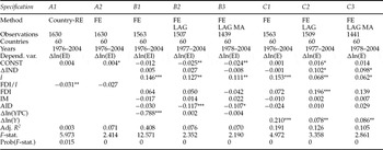
The results referring to specifications A, B, and C are reported in table 2.Footnote 20 Due to potential endogeneity in specification B1, we favor specifications B2 and B3. When computing significance levels, we always use heteroscedasticity-consistent covariances, since heteroscedasticity tests (Szroeter, Reference Szroeter1978; White, Reference White1980; Cook and Weisberg, Reference Cook and Weisberg1983) indicate heteroscedasticity in all cases. Testing for autocorrelation in panel data (Wooldridge, Reference Wooldridge2002; Drukker, Reference Drukker2003) on the other hand yields no clear indication for serial correlation in the residuals. However, since in some cases autocorrelation problems become obvious when regressing residuals on preceding residuals, we also use heteroscedasticity- and autocorrelation-consistent standard errors (Newey–West).
Estimation results for specifications A, B, and C

Notes: Heteroscedasticity and autocorrelation consistent standard errors; Δ = first time differences; Country-RE = country-specific random effects; FE = country- and time-specific fixed effects; LAG = lagged regressors; MA = the regressors FDI, IM, AID are moving averages of the past three years.
*Significant at the 10% level.
**Significant at the 5% level.
***Significant at the 1% level.
The F-tests for all coefficients jointly being zero reject the null hypothesis in all cases. However, the reported (adjusted) R 2 values are relatively low. One reason for the low explanatory power is that we estimate in first differences. The examination of the residuals’ distributions reveals in all cases very high Jarque–Bera statistics mainly stemming from high kurtosis values. Since this finding rejects the normal distribution assumption of the residuals, the reported significance levels should be interpreted with some caution. We could not remedy this problem by redefining the estimation model, changing the sample size, or eliminating outliers.
The coefficient of the variable of main interest, FDI inflows, is significant and negative in specification A1, which confirms the finding by Mielnik and Goldemberg (Reference Mielnik and Goldemberg2002). After slightly modifying specification A1 with time- and country-specific fixed effects to specification A2, the probability that the coefficient is different from zero already falls below any common significance level while the coefficient stays negative. In specification C2, where changes in total energy use are examined, the coefficient of lagged FDI inflows is positive and highly significant. According to the estimate, an increase of one percentage point in FDI intensity raises total energy supply by about 0.2 per cent. This finding is likely to stem from the scale effect: FDI inflows in the previous year induce increasing economic activity in the current year, which results in higher energy use. All other regressions do not confirm any significant effect of FDI on energy intensity. Using our theoretical background, the results imply that it is not possible to identify a robust energy-reducing effect of technology transfer via FDI in this macro panel.
We now compare the results for FDI with those for IM, AID and I. While imports do not show a significant effect in any regression, AID is significant and negative in specifications B2 and B3. This energy-intensity reduction by aid inflows is in line with the expectations that industrialized donor countries promote energy-saving technologies in developing countries. According to the results of B2, aid inflows amounting to 1 per cent of GDP of the recipient country reduce the country's energy intensity by about 0.1 per cent. On the contrary, the investment share in GDP labeled I is significantly positive in all specifications. Gross investment of 1 per cent of GDP increases energy intensity or total primary energy supply by about 0.1 per cent. The hypothesis that new capital investment brings about energy-saving technical progress is therefore challenged. It is on the other hand possible that the investment variable absorbs part of the composition effect: Since energy-intensive sectors are typically also capital intensive, a strong increase in investment may reflect an expansion of the energy intensive sectors and could therefore lead to an increase in energy intensity. This view is supported by the fact that our existing measure of the composition effect, namely, the share of industrial value added in GDP, is rather crude and cannot capture all sectoral changes in the economy.
Regarding the remaining control variables, income per-capita growth, Δln(YPC), is highly significant and negative in specification B1, but not in specifications B2 and B3 where it appears as a lagged variable. According to B1, a 1 per cent increase in per-capita income would reduce energy intensity by 0.79 per cent. This strong effect is likely to stem from short-term GDP fluctuations, where energy intensity, defined as energy supply over GDP, typically moves to the direction opposite that of GDP. If a longer-term influence really existed, we would find a significant result in specifications B2 or B3, but this is not the case. Furthermore, the significance of GDP per capita disappears also in specification B1 when the variable is instrumented by lagged GDP per capita as a robustness check. In models C1, C2, and C3, the change in total income, Δln(Y), has a significantly positive influence on total energy supply as expected (scale effect). The coefficient varies between 0.21 in C1 and 0.08 in C2. Concerning the share of industrial value added in GDP, we always find a positive sign, but the coefficient is significant only in specifications C2 and C3. It is likely that the sectoral change between the industry sector on the one hand and agriculture or services on the other hand is less important than sectoral changes within the industry sector. Unfortunately, no such detailed data are available for the countries in our sample; it is therefore possible that part of the composition effect is implicitly included in the coefficient of FDI.
We also extend the basic model (specification B) in order to investigate the interaction of FDI with country-specific characteristics. We add interaction terms of the aggregate FDI inflow intensity with changes in the share of industrial value added in GDP, with the import intensity and with shares of energy sources in total primary energy supply (particularly coal, oil, gas, nuclear power, and hydro power). The interaction of the FDI inflow intensity with the industry share in GDP examines whether FDI inflows coming along with changes in the sectoral composition influence the energy intensity in a country differently. Note that this interaction term includes the composition effect of FDI in the case of a systematic influence of FDI inflows on the industry share. The interaction of the FDI inflow intensity with the import intensity examines whether FDI and imports jointly affect the energy intensity due to increasing intra-firm imports by multinational enterprises. The interaction of the FDI inflow intensity with shares of energy sources determines whether the potential of FDI to affect energy intensity is related to the energy mix of a country. We run several regressions, including only one interaction term at the same time.Footnote 21 We find no evidence for an energy-reducing effect of the aggregate FDI inflow intensity, and none of the interaction terms leads to significant results. Nevertheless, the interaction term analyses show a way for further research, focusing more on the interactions of FDI with other economic indicators.
4. Robustness checks
In the robustness checks we address the following concerns: Technological improvements can foremost be expected from greenfield investment, i.e., installations of new production facilities and machinery, and not so much from pure ownership changes. Hence we correct our FDI data by subtracting mergers and acquisitions (M&A) in section 4.1. It would also be interesting to distinguish market-seeking horizontal FDI from low-production-cost-seeking vertical FDI, but such an empirical analysis is not possible due to a lack of data. Another reason for the inability to find any robust influence of FDI on energy intensity might be the fact that we use aggregated data without a distinction between sectors and between source countries of FDI. While FDI flows into energy-intensive sectors might have a significant potential for reducing economy-wide energy use, this might not be the case for FDI flows into other sectors. Furthermore, FDI from the United States might embody different technologies than FDI from Germany or Japan and therefore lead to other effects on energy use. In order to address these issues, we introduce new sectoral data for the United States as a source country of FDI in developing countries in section 4.2. Unfortunately, the robustness checks cannot be scrutinized with the full original data sample because of insufficient data availability. The price we have to pay is a reduced or modified sample in both robustness checks.
4.1. M&A correction of FDI
To get an approximation for greenfield investment, we subtract values of M&A from the FDI values we used before.Footnote 22 The M&A data are taken from UNCTAD (2008); the other data are the same as before. Due to a lack of data in the M&A database, the original sample is now reduced to the time frame of 1987–2004 and to 58 countries.Footnote 23
In general, the results confirm those found before (see table A5 in the online appendix at http://www.journals.cambridge.org/EDE). None of the specifications shows a significant energy-reducing effect of FDI. As with the original dataset, we find a significantly positive effect of the FDI intensity on the growth rate of total energy use in specification C2, which arises from the scale effect of FDI. The reduction of the growth rate of energy intensity via aid inflows can be confirmed in specifications B1, B2, and B3. Aid inflows of 1 per cent of GDP reduce energy intensity by about 0.06–0.19 per cent. The coefficient of aid is also significantly negative in C1 and C3. In contrast to the former regressions with the larger dataset, imports turn out to increase energy intensity in specifications B2 and B3. However, this effect is only weakly significant, both statistically and economically.
4.2. Sectoral data for the United States as a source country
Finally, we look specifically at FDI outflows from the United States and apply data from the Bureau of Economic Analysis (2008). Due to restricted data availability for the recipient countries we need to narrow the sample to 10 developing countriesFootnote 24 and four sectorsFootnote 25 from 1982 to 2003. Sectoral value-added data are taken from UNIDO (2006), and energy data are the International Energy Agency data as before. Both energy intensity and FDI in each country's sector are measured relative to the value added in the respective sector. In order to obtain consistent estimates for energy intensity, the value-added data are converted into constant purchasing-power parity values using the Penn World Table (Heston et al., Reference Heston, Summers and Aten2006) and a US consumer price index (International Monetary Fund, 2007b). We employ a parsimonious model specification in first time differences with the logarithm of energy intensity as the dependent variable and FDI as the only explanatory variable. In the second specification, we employ one-year lagged FDI values as the explanatory variable. We estimate a system of four equations, one for each sector, and apply the technique of seemingly unrelated regressions (SUR). This technique has the advantage that we gain separate results for each of the sectors. At the same time, it exploits the common information in the residuals across sectors and is therefore potentially more efficient than four separate regressions. We include a constant and estimate a pooled regression without fixed effects since the F-/LR-tests do not reject the null hypothesis of redundant fixed effects.
In the results (see table A6 in the online appendix at http://www.journals.cambridge.org/EDE), the coefficient of FDI inflows is not statistically significant in any of the sectors, and once again, the hypothesis of energy-saving technology transfer via FDI is not supported. Note that one reason for the inability to identify an energy-reducing technology effect might be a composition effect of FDI toward more energy-intensive products within the still aggregated sectors, i.e.,chemicals, food, machinery, and metals.
5. Conclusion
Referring to the hypothesis of energy-saving technology transfer proposed by Mielnik and Goldemberg (Reference Mielnik and Goldemberg2002), this paper examines whether FDI inflows reduce energy intensities of developing countries. Such reductions are desirable against the background of climate change mitigation, since energy use is strongly related to emissions of carbon dioxide. Theoretically, the impact of FDI inflows can be decomposed into a scale, a composition, and a technique effect (Grossman and Krueger, Reference Grossman, Krueger and Garber1993). Using the theoretical principles provided by Antweiler et al. (Reference Antweiler, Copeland and Taylor2001) and applying the concept to energy use, we set up an empirical macro-level model in order to identify the effects of technology transfer via FDI on energy intensities in developing countries.
We investigate cross-country panel data on 60 developing countries for the years 1975–2004. In the results, we find no energy-reducing effect of FDI inflows. Thus we cannot confirm the hypothesis of energy-saving technology transfer via FDI by Mielnik and Goldemberg (Reference Mielnik and Goldemberg2002) in general. Regarding the influence of foreign aid inflows on energy intensity, we find a significantly negative effect in several specifications. In order to take country-specific characteristics into account, we also examine the interaction of FDI inflows with changes in the industry share, with imports, and with shares of energy sources (particularly coal, oil, gas, nuclear power, and hydro power). We find no evidence for a significant joint effect of FDI inflows together with the other determinants on energy intensity. Finally, we carry out robustness checks with modified and new datasets. Correcting FDI inflow values by data on M&A as an approximation for greenfield investment confirms in general the original results. While energy savings via FDI cannot be found, the energy efficiency gains from foreign aid are confirmed. Focusing on the United States as a single source country and using sectorally disaggregated data, we find again no indication for energy savings via FDI.
However, there are caveats when interpreting the regression results. At first, the explanatory power of our model is low. On the one hand, this is caused by the loss of information due to differencing the estimating equation; on the other hand, the energy intensity of a country is determined by many technical, infrastructural, economic, and political factors that cannot all be captured in a macro model because the necessary data are not available. To consider as many unobservable effects as possible, we use panel data models with time- and country-specific effects. The second caveat is the high kurtosis of the residual distribution that biases the standard errors and consequently the significance levels. Reducing outliers from the sample and employing different model variants could not remedy this problem. If we restrict the study on time series of single countries, the vast heterogeneity in the sample would be reduced, and the properties of the residual distribution would be more favorable. Then, however, it would no longer be possible to derive general results. Finally, it is possible that while some FDI might reduce energy intensity via technology transfer, other FDI might induce a shift toward more energy-intensive production via a change in the sectoral composition of production. The significance of the results thus possibly suffers from the fact that we cannot fully disentangle technology transfer from the composition effect.
Nevertheless, our results suggest that energy efficiency gains in developing countries via FDI do not occur automatically and without climate or energy policy. Thus, it is sensible to make use of issue linkage, as for instance intended by the Clean Development Mechanism (CDM) of the Kyoto Protocol (for technology transfer in CDM projects, see Seres, Reference Seres2008) or international energy technology collaboration (Justus and Philibert, 2004), to explicitly encourage FDI that brings along energy-reducing technology transfer. A technology fund governed by the World Bank may also help to direct investment into energy-saving projects in developing countries. Note furthermore that our results could change in the presence of a carbon price in the countries under scrutiny, since pricing carbon creates an incentive to invest into energy-saving technologies.
A challenge for further research is to identify country-specific characteristics that enhance technology transfer via FDI. This can be accomplished by using interaction terms of FDI and country-specific variables. Departing from the panel analysis, it can be helpful to use data on specific countries in order to analyze whether FDI inflows reduce energy intensity in these specific cases. There is a broad literature on technology spillovers in general, but technology spillovers affecting energy intensity have not been investigated in depth. One can include long-run effects to examine whether spillovers from FDI decrease energy intensity with a time delay. Where sectoral data is available, the analysis can be performed in a more detailed way, and one can try to distinguish explicitly the composition effect from the technology transfer. A better understanding of international technology diffusion in the context of climate change is highly important for supporting developing countries in achieving lower energy and carbon intensities than the industrialized countries did in the past.