1 Introduction
The flow of a low-viscosity fluid through a permeable network composed of a more viscous fluid exists in a variety of geophysical contexts. Past studies of flow in viscously deformable porous media (VDPM) have tended to focus narrowly on constant-density, buoyancy-driven flows such as melt percolation in the upper mantle (McKenzie Reference McKenzie1984; Scott & Stevenson Reference Scott and Stevenson1984, Reference Scott and Stevenson1986; Spiegelman Reference Spiegelman1993a
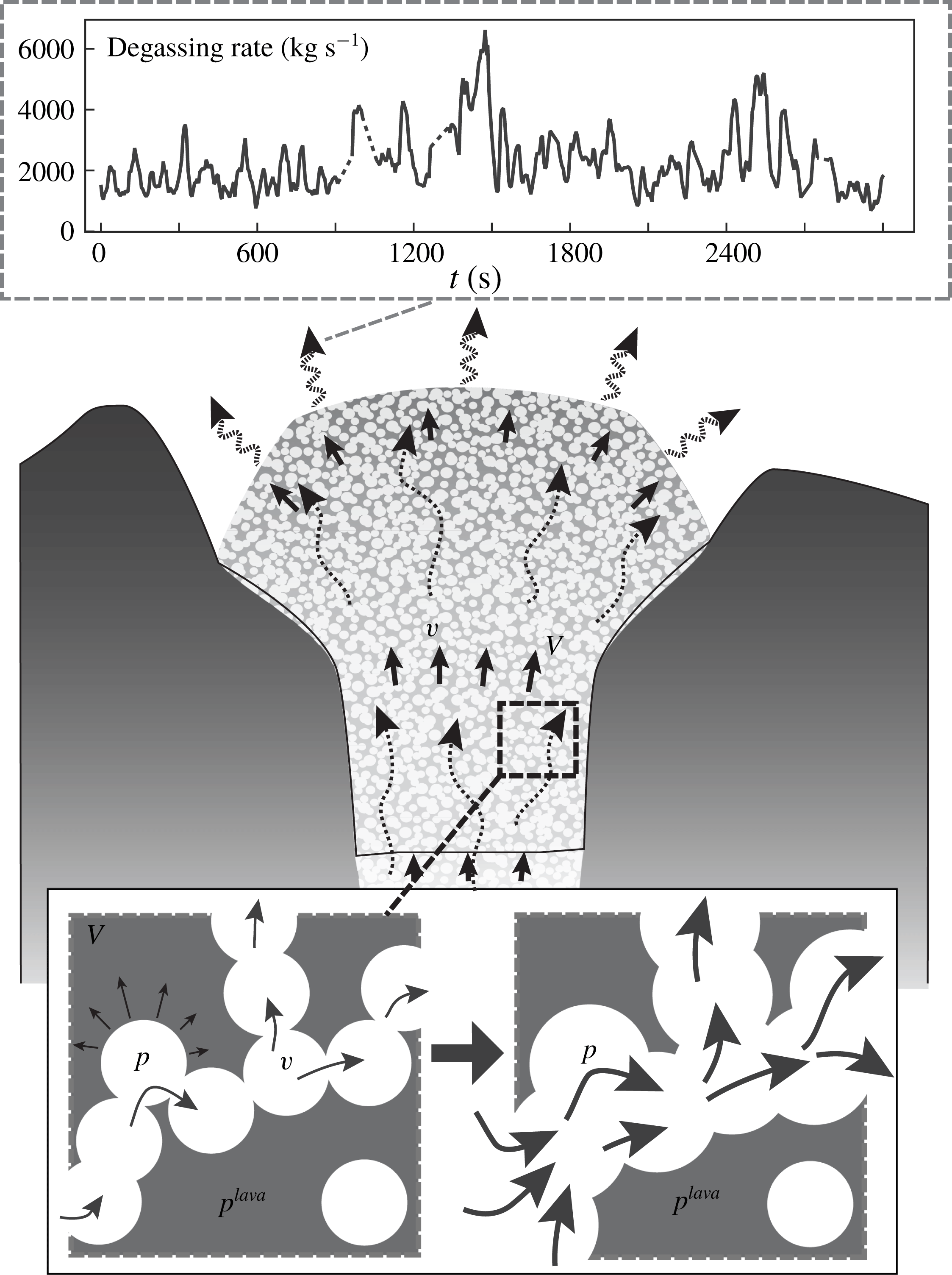
; Lowman & Hoefer Reference Lowman and Hoefer2013). However, pressure-driven compressible pore-fluid flows in VDPM comprise many important problems among geophysical flows including volatile hydrocarbon extraction from compacting sedimentary beds, the flow of gases and mud slurries in mud volcanoes and flow of magmatic gases and lava in a variety of volcanic settings. In particular, lava domes – highly viscous extrusions of lava which build up above a volcanic conduit – represent a type of pressure-driven gas flow in a VDPM with particular properties convenient for analysis. These are the flows analysed in this study (figure 1). It is clear from observations of passive, diffuse degassing (e.g. Delgado-Granados et al.
Reference Delgado-Granados, Cardenas-Gonzalez and Piedad-Sanchez2001) that growing lava domes typically host networks of microcracks and bubbles which allow some pressure to relax by porous flow. Indeed, by the time gas-rich magma reaches the surface to form a lava dome, it has long since passed the transition between bubble-dominated flow and permeable flow (Kozono & Koyaguchi Reference Kozono and Koyaguchi2010). This results in an effective porous network which may deform and is sufficiently viscous to resist significant buoyancy-driven bubble rise. Analyses of gas bubbles in lava based on percolation theory in these media suggest the use of a power law in relating porosity (
 $\unicode[STIX]{x1D719}$
) to permeability (
 $k$
) with a percolation threshold below which the medium becomes impermeable (Blower Reference Blower2001; Mueller et al.
Reference Mueller, Melnik, Spieler, Scheu and Dingwell2005; Vasseur & Wadsworth Reference Vasseur and Wadsworth2017). To study permeability breakdown in these flows we adopt the percolation relationship between the permeability (
 $k$
) and porosity (
 $\unicode[STIX]{x1D719}$
) suggested by Blower (Reference Blower2001):
 $$\begin{eqnarray}\displaystyle k(\unicode[STIX]{x1D719})=k_{0}(\unicode[STIX]{x1D719}-\unicode[STIX]{x1D719}_{c})_{+}^{b}:=\left\{\begin{array}{@{}ll@{}}k_{0}(\unicode[STIX]{x1D719}-\unicode[STIX]{x1D719}_{c})^{b}\quad & \unicode[STIX]{x1D719}_{c}<\unicode[STIX]{x1D719}<1\\ 0\quad & \text{otherwise},\end{array}\right. & & \displaystyle\end{eqnarray}$$
where
 $k_{0}$
is a coefficient related to the mean bubble radius (
 $r_{b}$
) by
 $k_{0}\approx 0.13\,r_{b}^{2}$
,
 $\unicode[STIX]{x1D719}_{c}$
is the percolation threshold which is typically taken as 0.3 and
 $b$
is an empirical exponent taken as 2.1. The presence of a percolation threshold will have critical implications for the development of shock waves where the matrix becomes impermeable. Above the percolation threshold, the specific parameter values in this model are not expected to influence the broad behaviour of the system as long as
 $\text{d}k/\text{d}\unicode[STIX]{x1D719}>0$
(Spiegelman Reference Spiegelman1993a
). In this context, the gases flowing through the lava are driven mainly by large pressure gradients imposed by the ambient atmospheric pressure condition at the surface. As a result, lava domes represent an important boundary layer at the surface of many volcanic systems. In general, many volcanic hazards including lava dome collapse, the generation of dense pyroclastic currents, or sudden explosions may be attributed to the breakdown of this boundary layer.
Conceptual model of the two-phase flow of gas and lava in a lava dome. Main figure shows a schematic representation of volcanic gases flowing through a permeable lava dome which is itself slowly flowing. Magnified figure is a schematic representation of the connection between local pore pressurization, matrix flow and porosity increase. Inset figure shows the short-term periodicity of degassing measured with forward-looking infrared (FLIR) images at Volcán Popocatépetl over
 ${\sim}50$
minutes (Hyman et al.
Reference Hyman, Bursik and Legorreta Paulin2018).

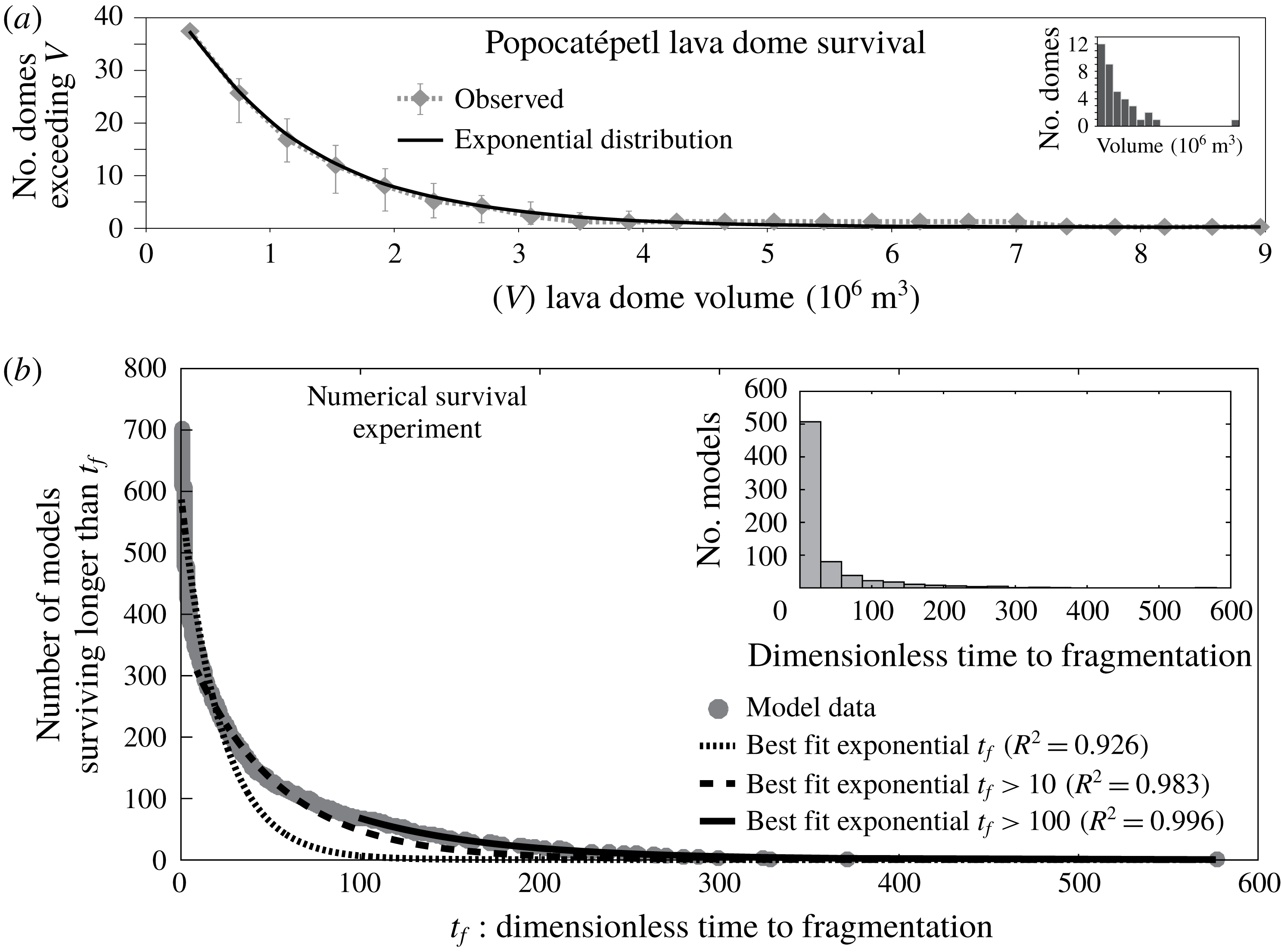
Periods of lava dome growth are very common and typically consist of one or more cycles of dome growth, collapse and explosive destruction (Yokoyama Reference Yokoyama2005). Because the strength of the dome is a function of the overburden, the pore pressure required to fracture the porous medium is smaller for smaller domes. Consequently, smaller domes pose less resistance to explosive breakup for a given pore pressure, which may explain the observation that rapid cycling of dome building and explosion tends to characterize the early phases of lava dome eruptions (Boudon et al. Reference Boudon, Balcone-Boissard, Villemant and Morgan2015). In the past two decades, Volcán Popocatépetl, Mexico has become a type example for this behaviour, having extruded and destroyed at least 38 small lava domes between 1996 and 2016 (Gómez-Vazquez, De la Cruz-Reyna & Mendoza-Rosas Reference Gómez-Vazquez, De la Cruz-Reyna and Mendoza-Rosas2016). Recent analysis of the sizes and residence times of these domes has led to the generation of a ‘survival curve’ for the ongoing lava dome eruptive period at Popocatépetl showing that the number of domes surviving to a given size decays exponentially with increasing lava dome volume, that is, domes are more likely to be destroyed by explosions early in their extrusion, limiting the number of domes that can survive to a large size (Gómez-Vazquez et al. Reference Gómez-Vazquez, De la Cruz-Reyna and Mendoza-Rosas2016). Given that the uncertainty in lava parameters such as viscosity and permeability varies over several orders of magnitude at Popocatépetl and other volcanoes, any attempt to model the long-time behaviour of lava dome eruptions should sample over many orders of magnitude and should show a consistent ensemble model behaviour. Because of the availability of dome survival data from Popocatépetl, this work seeks to construct an adequate numerical experiment of dome survival, the results of which may be combined and compared with these data to explain patterns in the long term cyclicity of lava dome extrusion and destruction. Owing to this cyclic behaviour, Popocatépetl provides an excellent natural example for comparison with the theory developed here.
Recent studies of magmatic degassing have shown that gas flow has significant periodicity with dominant oscillation periods in the range
 $O(10^{2}){-}O(10^{3}~\text{s})$
across a wide variety of volcanic settings representing a range of lava compositions and physical parameterizations. These include periods of 40–250 s and 500–1200 s at Mt. Etna, Italy (Tamburello et al.
Reference Tamburello, Aiuppa, McGonigle, Allard, Cannata, Giudice, Kantzas and Pering2013),
 ${\sim}600$
s at the Mt. Erebus lava lake, Antarctica (Sweeney et al.
Reference Sweeney, Kyle and Oppenheimer2008), 300–600 s at Santiaguito lava dome complex, Guatemala (Holland et al.
Reference Holland, Watson, Phillips, Caricchi and Dalton2011), 100–2000 s at Mayon Volcano, Philippines (Girona et al.
Reference Girona, Costa, Taisne, Aggangan and Ildefonso2015) and
 ${\sim}100$
–1000 s at Volcán Popocatépetl, Mexico (figure 1 inset, Hyman et al. (Reference Hyman, Bursik and Legorreta Paulin2018)). Overall, these measurements suggest that the flux of gas through a lava dome is oscillatory, providing a natural time scale with which to study the dynamics of lava dome gas flow. The short duration of this natural time scale with respect to viscous relaxation time scales in the matrix will allow for important simplifications in the governing equations including an approximately stationary matrix phase.
As in previous studies of VDPM, the compaction length of these flows exerts a strong control on the dynamics of the system. Generally, the compaction length is a combination of the matrix permeability, the matrix viscosity and the pore-fluid viscosity which together form a natural length scale in these problems. As originally defined by McKenzie (Reference McKenzie1984), the compaction length is a natural length scale in the simplified problem of a saturated porous medium compacting onto an impermeable lower boundary. In that context, McKenzie (Reference McKenzie1984) defined the compaction length
 $\unicode[STIX]{x1D6FF}$
as the distance from the impermeable boundary over which the compaction rate decays by a factor of
 $e$
. Despite the simplicity of this problem, the compaction length as a combination of model parameters is widely used as a natural length scale in studies of compacting porous media outside the bounds of this specific mathematical definition. Although studies of melt percolation in the upper mantle have considered compaction and expansion due to isotropic and shear stresses, in this study, we consider only isotropic compaction and expansion of a free-surface VDPM in one dimension, effectively ignoring the effects of shear near the crater walls. Because of this simplification and the form of the
 $k-\unicode[STIX]{x1D719}$
relationship used here, we define the compaction length in this study as
 $\unicode[STIX]{x1D6FF}=\sqrt{k_{0}\unicode[STIX]{x1D701}/\unicode[STIX]{x1D707}}$
, where
 $\unicode[STIX]{x1D707}$
is the pore-fluid dynamic viscosity and
 $\unicode[STIX]{x1D701}$
is the bulk viscosity of the matrix. Owing to the lack of data for this parameter in a volcanic context, we take this to be the same order of magnitude as the matrix shear viscosity. In the study of a free-surface VDPM, the role of the compaction length in the flow dynamics will be affected by the thickness of the flow. In the present study, that thickness is the dome height above the top of the conduit. As a result, there are two natural length scales of the problem: the dome thickness and compaction length. This will generate a parameterization of the flow with small differences from previous studies of VDPM where the relationship between compaction length and dome thickness will control the flow behaviour. The most important simplification arising in this study of gas flow in VDPM applied to lava domes is that these domes may be treated as slow-moving gravity currents and thus the lava matrix phase pressure is approximated as magmastatic, yielding space-dependent source terms in the resulting governing equations.
In the present study, we show that consideration of a compressible pore fluid leads directly to a two-equation mixed hyperbolic–parabolic system describing a diverse suite of behaviours including nonlinear wave-diffusion behaviour.
Previous studies of flow in VDPM have focused on cases where the pore and matrix fluids are incompressible, which has generally led to nonlinear equations governing the pore fluid fraction or porosity. Despite the dominance of viscous processes and thus low Reynolds number in these flows, the governing equations derived in previous studies describe non-dissipative flow phenomena such as dispersive and non-dispersive shock waves (Spiegelman Reference Spiegelman1993a ,Reference Spiegelman b ; Lowman & Hoefer Reference Lowman and Hoefer2013). In particular, the problem of upper-mantle melt percolation has led to the development of a single governing equation for the porosity describing nonlinear dispersive wave phenomena and is typically called the ‘magma equation’ (Lowman & Hoefer Reference Lowman and Hoefer2013). In this context, buoyancy of the percolating phase with respect to the matrix phase drives the flow. In previous studies of compressible pore-fluid flows in VDPM, the focus has typically been two-phase gas–lava flows. In this application, the lava–gas viscosity ratio has typically been significantly lower than the mantle rock–magma viscosity ratio in classical VDPM theory. As a result, the fluid dynamics of the matrix phase has played a significant role in studies of gas–lava VDPM flows (Melnik & Sparks Reference Melnik and Sparks1999; Costa et al. Reference Costa, Melnik, Sparks and Voight2007; Michaut et al. Reference Michaut, Ricard, Bercovici and Sparks2013). In particular, Michaut et al. (Reference Michaut, Ricard, Bercovici and Sparks2013) in studying wave dynamics of the system, derived governing equations for the flow of gas in permeable lava in a volcanic conduit which described the behaviour of the gas density, lava porosity, gas velocity and variable lava velocity. However, that study failed to produce an equilibrium solution to the derived equations and instead constructed a non-equilibrium background state. Consequently, upon performing a linearization, the background states considered led to linear equations with variable coefficients into which an unjustified plane-wave ansatz was substituted despite such equations requiring alternative methods of linear stability analysis. Despite this, the authors suggested that the resulting dispersion relation showed that the flow of gas and lava is unstable and that the excited gas wave periodicity compared well with observations of lava dome growth and instability from Soufrière Hills volcano, Montserrat. Overall, the good agreement between that model and natural data, despite the mathematical errors, has made the study of the wave dynamics of gas flow in viscous lavas less clear.
The purpose of this study is to extend and adapt VDPM theory to the pressure gradient-driven flow of compressible pore fluids with specific application to understanding gas flow in lava domes. This is presented as follows: we begin with the general equations of motion in VDPM and introduce various simplifying assumptions related to the specific problem of gas flow in lava domes including that of an isothermal ideal gas and the magmastatic lava pressure condition. In doing so, we show that the isothermal pore-fluid compressibility generates a parabolic partial differential equation (PDE) governing nonlinear diffusion of pore pressure which is modulated by compaction due to porosity wave motion. We then present several solutions to limiting cases in one dimension including spatially variable steady-state pressure and porosity profiles and show that these steady states are conditionally stable dependent on several physical parameters of the flow. From this analysis we show that numerical solutions contain both diffusion-type and nonlinear wave-type behaviour. In particular, we highlight the formation of shock waves in connection to the development of permeable–impermeable transitions. Lastly, we perform a numerical experiment showing that lava dome fragmentation is predicted in agreement with natural lava dome survival data from Volcán Popocatépetl, Mexico.
2 Governing equations for gas flow in a deforming lava dome
In the following, we consider a simplified model of lava dome gas flow in which the gas is assumed to percolate by permeable flow through the deforming pore network of the lava dome at constant temperature with negligible mass exchange between lava and gas. In this model, we assume that the bulk compressibility of the lava–gas mixture is due to changes in porosity and gas pressure and that the liquid phase is incompressible. The governing equations can then be written after Spiegelman (Reference Spiegelman1993a ), Blower (Reference Blower2001) as
 $$\begin{eqnarray}\displaystyle & \displaystyle \unicode[STIX]{x2202}_{t}(\unicode[STIX]{x1D719}\unicode[STIX]{x1D70C}^{gas})+\unicode[STIX]{x1D735}\boldsymbol{\cdot }(\unicode[STIX]{x1D719}\unicode[STIX]{x1D70C}^{gas}\boldsymbol{v})=0 & \displaystyle\end{eqnarray}$$
 $$\begin{eqnarray}\displaystyle & \displaystyle \unicode[STIX]{x1D70C}^{lava}\,\unicode[STIX]{x2202}_{t}(1-\unicode[STIX]{x1D719})+\unicode[STIX]{x1D70C}^{lava}\unicode[STIX]{x1D735}\boldsymbol{\cdot }((1-\unicode[STIX]{x1D719})\boldsymbol{V})=0 & \displaystyle\end{eqnarray}$$
 $$\begin{eqnarray}\displaystyle & \displaystyle \unicode[STIX]{x1D719}(\boldsymbol{v}-\boldsymbol{V})=-\frac{k(\unicode[STIX]{x1D719})}{\unicode[STIX]{x1D707}}\unicode[STIX]{x1D735}p & \displaystyle\end{eqnarray}$$
 $$\begin{eqnarray}\displaystyle & \displaystyle k(\unicode[STIX]{x1D719})=k_{0}(\unicode[STIX]{x1D719}-\unicode[STIX]{x1D719}_{c})_{+}^{b} & \displaystyle\end{eqnarray}$$
 $$\begin{eqnarray}\displaystyle & \displaystyle \unicode[STIX]{x1D70C}^{gas}=p/RT^{dome}, & \displaystyle\end{eqnarray}$$
 $\unicode[STIX]{x1D719}$
is the porosity of the dome lava,
 $\unicode[STIX]{x1D70C}^{()}$
is the phase density,
 $\boldsymbol{v}$
and
 $\boldsymbol{V}$
are respectively the gas and lava velocities,
 $k$
is the lava permeability,
 $\unicode[STIX]{x1D707}$
is the gas viscosity,
 $p$
is the gas pressure,
 $R$
is the specific gas constant and
 $T^{dome}$
is the temperature of the dome, assumed to be constant and equal for the gas and lava. Equations (2.1a
) and (2.1b
) express conservation of mass for the gas and lava phases respectively. Equation (2.1c
) is a co-moving form of Darcy’s law which constitutes an equation for the conservation of momentum of the gas.
For momentum conservation in the lava, we take the lava pressure to be magmastatic, given by
 $p^{lava}=p_{a}+\unicode[STIX]{x1D70C}^{lava}g(h-z)$
, where
 $p_{a}$
is atmospheric pressure at the lava dome surface and
 $z=h$
is the surface of the dome, which may vary horizontally. Furthermore, we simplify the compressibility of the bulk lava with a linear rheological assumption. This is expressed as
 $$\begin{eqnarray}\displaystyle \unicode[STIX]{x1D701}\unicode[STIX]{x1D735}\boldsymbol{\cdot }\boldsymbol{V}=p-p^{lava} & & \displaystyle\end{eqnarray}$$
after Scott & Stevenson (Reference Scott and Stevenson1986), where
 $\unicode[STIX]{x1D701}$
is the bulk viscosity of the lava medium, typically estimated as the same order of magnitude as the dynamic viscosity. This relation couples the lava and gas pressures and describes compression and expansion of the lava–gas mixture (figure 1).
2.1 Combined equations
We combine all of the above equations into a set of two governing equations:
 $$\begin{eqnarray}\displaystyle & \displaystyle \unicode[STIX]{x1D719}\frac{\text{D}p}{\text{D}t}=\frac{k_{0}}{\unicode[STIX]{x1D707}}\unicode[STIX]{x1D735}\boldsymbol{\cdot }[(\unicode[STIX]{x1D719}-\unicode[STIX]{x1D719}_{c})_{+}^{b}p\unicode[STIX]{x1D735}p]-\frac{1}{\unicode[STIX]{x1D701}}p(p-p^{lava}) & \displaystyle\end{eqnarray}$$
 $$\begin{eqnarray}\displaystyle & \displaystyle \frac{\text{D}\unicode[STIX]{x1D719}}{\text{D}t}=\frac{1}{\unicode[STIX]{x1D701}}(1-\unicode[STIX]{x1D719})(p-p^{lava}), & \displaystyle\end{eqnarray}$$
 $\text{D}/\text{D}t=\unicode[STIX]{x2202}/\unicode[STIX]{x2202}t+\boldsymbol{V}\boldsymbol{\cdot }\unicode[STIX]{x1D735}$
is the Lagrangian derivative. Apart from advection, which will be shown to be negligible, the system consists of a nonlinear diffusion–reaction type PDE coupled to a first-order ordinary differential equation (ODE) describing evolution of the porosity field.
To non-dimensionalize this system, we use the transformation
 $$\begin{eqnarray}\displaystyle \left.\begin{array}{@{}c@{}}p^{\ast }=p/p_{0};\quad \boldsymbol{V}^{\ast }=\boldsymbol{V}/V_{c};\quad \boldsymbol{x}^{\ast }=\boldsymbol{x}/h_{0};\quad t^{\ast }=t/t_{c};\\ h^{\ast }=h/h_{0};\quad f=p^{lava}/p_{0}=f_{a}+h^{\ast }-z^{\ast },\end{array}\right\} & & \displaystyle\end{eqnarray}$$
where
 $h_{0}$
is the maximum dome height,
 $p_{0}=\unicode[STIX]{x1D70C}^{lava}gh_{0}$
is the maximum lava pressure at the base of the dome,
 $f_{a}=p_{a}/p_{0}$
is the non-dimensional ambient air pressure,
 $f$
represents the non-dimensional lava pressure and
 $V_{c}$
and
 $t_{c}$
are scale factors for the lava velocity and time respectively. This yields a non-dimensional system (with stars dropped) where
 $p$
,
 $\unicode[STIX]{x1D719}$
,
 $\boldsymbol{x}$
,
 $t$
,
 $\boldsymbol{V}$
and
 $f$
are now
 $O(1)$
dimensionless variables:
 $$\begin{eqnarray}\displaystyle & \displaystyle \unicode[STIX]{x1D719}(\unicode[STIX]{x2202}_{t}p+\unicode[STIX]{x1D712}\boldsymbol{V}\boldsymbol{\cdot }\unicode[STIX]{x1D735}p)=\unicode[STIX]{x1D6FC}\unicode[STIX]{x1D735}\boldsymbol{\cdot }[(\unicode[STIX]{x1D719}-\unicode[STIX]{x1D719}_{c})_{+}^{b}p\unicode[STIX]{x1D735}p]-\unicode[STIX]{x1D6FD}p(p-f) & \displaystyle\end{eqnarray}$$
 $$\begin{eqnarray}\displaystyle & \displaystyle \unicode[STIX]{x2202}_{t}\unicode[STIX]{x1D719}+\unicode[STIX]{x1D712}\boldsymbol{V}\boldsymbol{\cdot }\unicode[STIX]{x1D735}\unicode[STIX]{x1D719}=\unicode[STIX]{x1D6FD}(1-\unicode[STIX]{x1D719})(p-f) & \displaystyle\end{eqnarray}$$
 $$\begin{eqnarray}\displaystyle \unicode[STIX]{x1D712}=\frac{V_{c}t_{c}}{h_{0}};\quad \unicode[STIX]{x1D6FC}=\frac{k_{0}p_{0}t_{c}}{\unicode[STIX]{x1D707}h_{0}^{2}};\quad \unicode[STIX]{x1D6FD}=\frac{p_{0}t_{c}}{\unicode[STIX]{x1D701}}. & & \displaystyle\end{eqnarray}$$
Typical lava dome volumetric flow rates are
 ${\sim}1{-}10~\text{m}^{3}~\text{s}^{-1}$
, implying that for typical lava dome volumes (
 $O(10^{6}){-}O(10^{8})~\text{m}^{3}$
), the mean velocity throughout a dome is only
 $O(10^{-5}){-}O(10^{-4})~\text{m}~\text{s}^{-1}$
(Sheldrake et al.
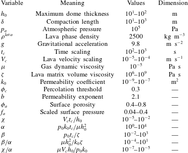
Reference Sheldrake, Sparks, Cashman, Wadge and Aspinall2016). For typical values of the parameters in
 $\unicode[STIX]{x1D712}$
,
 $\unicode[STIX]{x1D6FC}$
and
 $\unicode[STIX]{x1D6FD}$
the diffusion and compaction terms are much stronger than the advection term (table 1). Therefore we neglect the advection and take the limit
 $\unicode[STIX]{x1D712}\rightarrow 0$
throughout the present study. This limit simplifies (2.5a
) and (2.5b
) to a system of two equations for two unknown fields: the pressure
 $p$
and porosity
 $\unicode[STIX]{x1D719}$
.
Values of parameters used including ranges where uncertain.

2.2 One-dimensional analysis
We will consider a simplified version of these combined equations: purely vertical gas flow, casting the equations over only the vertical coordinate and time as
 $$\begin{eqnarray}\displaystyle & \displaystyle \unicode[STIX]{x1D719}\,\unicode[STIX]{x2202}_{t}p=\unicode[STIX]{x1D6FC}\,\unicode[STIX]{x2202}_{z}[K(\unicode[STIX]{x1D719})p\,\unicode[STIX]{x2202}_{z}p]-\unicode[STIX]{x1D6FD}p(p-f) & \displaystyle\end{eqnarray}$$
 $$\begin{eqnarray}\displaystyle & \displaystyle \unicode[STIX]{x2202}_{t}\unicode[STIX]{x1D719}=\unicode[STIX]{x1D6FD}(1-\unicode[STIX]{x1D719})(p-f), & \displaystyle\end{eqnarray}$$
 $K(\unicode[STIX]{x1D719})=(\unicode[STIX]{x1D719}-\unicode[STIX]{x1D719}_{c})_{+}^{b}$
is the non-dimensional permeability. In addition to these governing equations, we implement the following boundary conditions:
 $$\begin{eqnarray}\displaystyle & \displaystyle p=f_{a}\quad \text{on }\{z=1\}\times [0,\infty ] & \displaystyle\end{eqnarray}$$
 $$\begin{eqnarray}\displaystyle & \displaystyle K(\unicode[STIX]{x1D719})p\,\unicode[STIX]{x2202}_{z}p=-\unicode[STIX]{x1D6EC}_{s}Q(t)\quad \text{on }\{z=0\}\times [0,\infty ], & \displaystyle\end{eqnarray}$$
 $$\begin{eqnarray}\displaystyle \unicode[STIX]{x1D6EC}_{s}=\frac{{\dot{m}}_{s}\unicode[STIX]{x1D707}RT^{dome}}{\unicode[STIX]{x1D70C}^{2}g^{2}h_{0}k_{0}A}, & & \displaystyle\end{eqnarray}$$
which represent a constant ambient pressure at the dome surface and some flux of gas from the lower boundary (volcanic conduit) which is
 $\unicode[STIX]{x1D6EC}_{s}$
during steady-state conditions and varies from steady state according to
 $Q(t)$
. The lower boundary condition is given here in a general form to be detailed later. These simplified equations represent a coupled system in which the diffusion of gas pressure is modified by changes in the porosity and permeability due to expansion and compression of the porous lava medium. This compaction is itself dependent on the gas–lava pressure difference. Equation (2.7a
) is a nonlinear parabolic PDE which becomes singular in both of the limits
 $p\rightarrow 0^{+}$
and
 $\unicode[STIX]{x1D719}\rightarrow \unicode[STIX]{x1D719}_{c}^{+}$
. The first limit is a common degeneracy and is related to the similarity between (2.7a
) and the equation governing porous flow of gases in a rigid network, the so-called porous medium equation (PME). Generally, the PME yields nonlinear diffusion due to pressure-proportional diffusivity resulting in steeper pressure gradients than linear diffusion and finite propagation speed (Vazquez Reference Vazquez2007). In the present context, the
 $p\rightarrow 0$
limit is unphysical; however, porosities below the percolation threshold are found widely in lava dome samples (Boudon et al.
Reference Boudon, Balcone-Boissard, Villemant and Morgan2015) and so the second limit (
 $\unicode[STIX]{x1D719}\rightarrow \unicode[STIX]{x1D719}_{c}$
) is physically relevant. If
 $\unicode[STIX]{x1D719}\leqslant \unicode[STIX]{x1D719}_{c}$
, equations (2.7a
) and (2.7b
) can be combined as
 $$\begin{eqnarray}\displaystyle \frac{\unicode[STIX]{x2202}_{t}p}{p}=\frac{\unicode[STIX]{x2202}_{t}\unicode[STIX]{x1D719}}{\unicode[STIX]{x1D719}(1-\unicode[STIX]{x1D719})} & & \displaystyle\end{eqnarray}$$
and integrated to find a phase-plane solution:
 $$\begin{eqnarray}\displaystyle p(z,t)=p_{c}(z)\frac{\unicode[STIX]{x1D719}_{c}}{1-\unicode[STIX]{x1D719}_{c}}\left[\frac{1-\unicode[STIX]{x1D719}(z,t)}{\unicode[STIX]{x1D719}(z,t)}\right], & & \displaystyle\end{eqnarray}$$
where
 $p_{c}(z)$
is the local pore pressure when the porosity drops below the percolation threshold or
 $p_{c}(z)=p(z;\unicode[STIX]{x1D719}=\unicode[STIX]{x1D719}_{c})$
. Although there is no closed-form solution for
 $p$
and
 $\unicode[STIX]{x1D719}$
in terms of
 $z$
and
 $t$
only, this relation indicates that in a hydraulically unconnected region, the pressure and porosity are inversely related, that is, when the porosity drops below the percolation threshold due to a negative pressure anomaly (
 $p-f<0$
), the porosity will continue to contract, causing the pressure to rise back to
 $p=f$
.
Additionally, equations (2.7a
) and (2.7b
) have three steady-state solutions (
 $p_{s}(z)$
,
 $\unicode[STIX]{x1D719}_{s}(z)$
), although only one is physical and allows porous gas flow:
 $$\begin{eqnarray}\displaystyle & \displaystyle p_{s}(z)=f(z)=f_{a}+1-z & \displaystyle\end{eqnarray}$$
 $$\begin{eqnarray}\displaystyle & \displaystyle \unicode[STIX]{x1D719}_{s}(z)=\unicode[STIX]{x1D719}_{c}+\left[\frac{\unicode[STIX]{x1D6EC}_{s}}{f(z)}\right]^{1/b}, & \displaystyle\end{eqnarray}$$
 $\unicode[STIX]{x1D6EC}_{s}$
is the dimensionless Darcy flux,
 ${\dot{m}}_{s}$
is the steady-state mass flow rate of gas through the dome and
 $A$
is the dome cross-sectional area. The values of the parameters in
 $\unicode[STIX]{x1D6EC}_{s}$
are restricted in the sense that the porosity must remain physically bounded (
 $0\leqslant \unicode[STIX]{x1D719}\leqslant 1$
). Because the steady-state porosity profile increases towards the surface, we define an additional parameter (
 $\unicode[STIX]{x1D719}_{a}$
), the ‘surface porosity’ of the lava dome as
 $$\begin{eqnarray}\displaystyle \unicode[STIX]{x1D719}_{a}=\unicode[STIX]{x1D719}_{c}+\left(\frac{\unicode[STIX]{x1D6EC}_{s}}{f_{a}}\right)^{1/b}=\unicode[STIX]{x1D719}_{c}+\left(\frac{{\dot{m}}_{s}\unicode[STIX]{x1D707}RT^{dome}}{p_{a}\unicode[STIX]{x1D70C}^{lava}gk_{0}A}\right)^{1/b}. & & \displaystyle\end{eqnarray}$$
To find physically reasonable values of the flux
 $\unicode[STIX]{x1D6EC}_{s}$
, the parameters must be constrained such that
 $\unicode[STIX]{x1D719}_{c}<\unicode[STIX]{x1D719}_{a}(\unicode[STIX]{x1D6EC}_{s})<1$
.
The exact form of the porosity steady-state solution is governed by the
 $k-\unicode[STIX]{x1D719}$
relationship. Although
 $K(\unicode[STIX]{x1D719}_{s})\propto 1/f$
in general, the exact form of
 $\unicode[STIX]{x1D719}_{s}(z)$
will depend upon inverting the particular
 $K(\unicode[STIX]{x1D719})$
for the problem. Consideration of other porosity–permeability relationships is beyond the scope of this work.
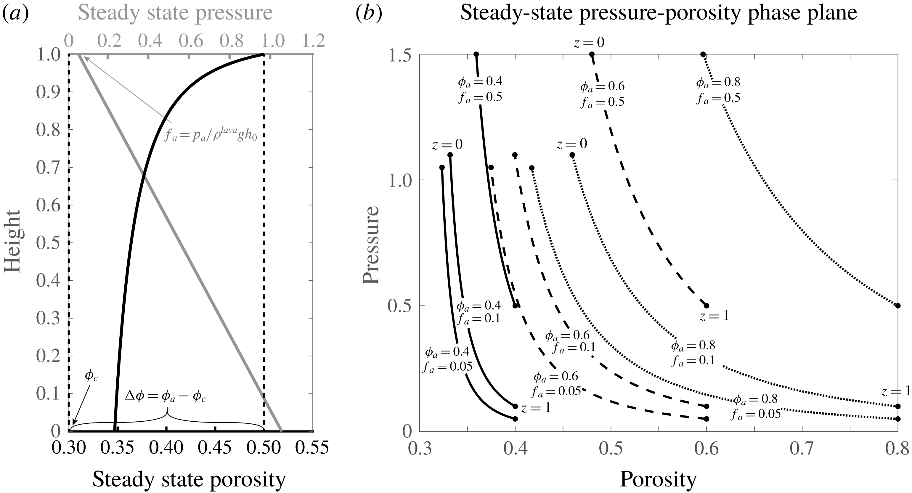
These solutions indicate a magmastatic steady-state pore gas pressure and that the steady-state porosity profile accommodates this linear pressure increase by increased compaction with depth (figure 2
a). Furthermore, the dimensionless pressure gradient is always normalized as
 $\text{d}f/\text{d}z=-1$
regardless of the choice of the parameters
 $f_{a}$
and
 $\unicode[STIX]{x1D719}_{a}$
; however, the porosity profile changes significantly for different choices of these parameters (figure 2
b). Indeed, for small
 $f_{a}$
, the porosity profiles are most heavily curved, which can be seen as phase plane curves with the lowest values of
 $\text{d}p/\text{d}\unicode[STIX]{x1D719}$
(figure 2). The steady-state pressure plays a particularly important role for understanding how the transient equations evolve since the expansion and compaction terms of (2.7a
) and (2.7b
) are functions of the deviation from steady-state pressure, that is, perfect gas–lava pressure coupling.
(a) One-dimensional steady-state (equilibrium) profiles for gas pressure (non-dimensional) (grey) and porosity (black). (b) Variation of these profiles for different parameter values represented in the
 $p-\unicode[STIX]{x1D719}$
phase plane.
 $\unicode[STIX]{x1D719}_{a}=0.4$
(solid),
 $\unicode[STIX]{x1D719}_{a}=0.6$
(dashed),
 $\unicode[STIX]{x1D719}_{a}=0.8$
(dotted).

3 Linearization and wave growth analysis
We linearize
 $p,\unicode[STIX]{x1D719}$
around the steady-state profiles, now introducing two additional shorthand notations: the porosity contrast between the surface of the matrix and percolation threshold (
 $\unicode[STIX]{x0394}\unicode[STIX]{x1D719}=\unicode[STIX]{x1D719}_{a}-\unicode[STIX]{x1D719}_{c}$
) and the steady-state permeability
 $k_{s}(z)=\unicode[STIX]{x0394}\unicode[STIX]{x1D719}^{b}f_{a}/f(z)$
. For a small parameter
 $\unicode[STIX]{x1D716}$
, we substitute the ansatz
 $$\begin{eqnarray}\displaystyle \binom{p(z,t)}{\unicode[STIX]{x1D719}(z,t)}=\binom{p_{s}(z)}{\unicode[STIX]{x1D719}_{s}(z)}+\unicode[STIX]{x1D716}\binom{p^{(1)}(z,t)}{\unicode[STIX]{x1D719}^{(1)}(z,t)}+O(\unicode[STIX]{x1D716}^{2}) & & \displaystyle\end{eqnarray}$$
into (2.7a
) and (2.7b
) and take the limit
 $\unicode[STIX]{x1D716}\rightarrow 0$
.
3.1 Uniform background state
To examine the effects of the background state on the behaviour of perturbations, we first consider the assumption of a uniform background state that has typically been used in linear stability analyses (LSA) of similar gas–lava mixtures (Manga Reference Manga1996; Jellinek & Bercovici Reference Jellinek and Bercovici2011; Yarushina et al.
Reference Yarushina, Bercovici and Michaut2015). In this formulation,
 $f$
,
 $\unicode[STIX]{x1D719}_{s}$
and
 $k_{s}$
are taken as constants. This implies either of the unphysical conditions: depth-invariant lava pressure or zero lava dome thickness. However, we make this assumption to simplify the analysis and give insight into the contrast between the behaviour of the system under uniform and non-uniform background states which we examine in greater detail below. Following the linearization procedure yields
 $$\begin{eqnarray}\displaystyle & \displaystyle \unicode[STIX]{x1D719}_{s}\,\unicode[STIX]{x2202}_{t}p^{(1)}=\unicode[STIX]{x1D6FC}\unicode[STIX]{x0394}\unicode[STIX]{x1D719}^{b}f_{a}\,\unicode[STIX]{x2202}_{zz}p^{(1)}-\unicode[STIX]{x1D6FD}fp^{(1)} & \displaystyle\end{eqnarray}$$
 $$\begin{eqnarray}\displaystyle & \displaystyle \unicode[STIX]{x2202}_{t}\unicode[STIX]{x1D719}^{(1)}=\unicode[STIX]{x1D6FD}(1-\unicode[STIX]{x1D719}_{s})p^{(1)}, & \displaystyle\end{eqnarray}$$
 $p^{(1)},\unicode[STIX]{x1D719}^{(1)}$
are the scaled perturbations. A classical LSA for a parabolic system typically makes the ansatz of a plane-wave solution
 $(p^{(1)},\unicode[STIX]{x1D719}^{(1)})=\exp [\text{i}\unicode[STIX]{x1D705}z+\unicode[STIX]{x1D706}(\unicode[STIX]{x1D705})t]$
with constant wavenumber (
 $\unicode[STIX]{x1D705}$
) and then examines the form of the dispersion relation
 $\unicode[STIX]{x1D706}(\unicode[STIX]{x1D705})$
:
 $$\begin{eqnarray}\displaystyle \unicode[STIX]{x1D706}(\unicode[STIX]{x1D705})=-\frac{f}{\unicode[STIX]{x1D719}_{s}}(\unicode[STIX]{x1D6FC}k_{s}\unicode[STIX]{x1D705}^{2}+\unicode[STIX]{x1D6FD})\leqslant 0, & & \displaystyle\end{eqnarray}$$
which implies that for all physical values of the parameters, the background state is stable and perturbations will decay. Additionally, because
 $\unicode[STIX]{x1D706}$
is purely real, perturbations decay in place, eliminating any wave motion. However, the simplicity of a constant background state does not capture the reality of background gradients present in the steady-state solutions.
3.2 Non-uniform background state
Using the properties of the steady states (2.12a ), (2.12b ), the linearization ansatz yields (after much simplification)
 $$\begin{eqnarray}\displaystyle & \displaystyle \frac{1}{\unicode[STIX]{x1D6FC}}\,\unicode[STIX]{x2202}_{t}p^{(1)}=w_{p}\,\unicode[STIX]{x2202}_{z}p^{(1)}+w_{\unicode[STIX]{x1D719}}\,\unicode[STIX]{x2202}_{z}\unicode[STIX]{x1D719}^{(1)}+D_{p}\,\unicode[STIX]{x2202}_{zz}p^{(1)}+R_{pp}p^{(1)}+R_{p\unicode[STIX]{x1D719}}\unicode[STIX]{x1D719}^{(1)} & \displaystyle\end{eqnarray}$$
 $$\begin{eqnarray}\displaystyle & \displaystyle \frac{1}{\unicode[STIX]{x1D6FC}}\,\unicode[STIX]{x2202}_{t}\unicode[STIX]{x1D719}^{(1)}=R_{\unicode[STIX]{x1D719}p}p^{(1)}, & \displaystyle\end{eqnarray}$$
 $$\begin{eqnarray}\displaystyle & \displaystyle \unicode[STIX]{x2202}_{z}p^{(1)}=0\quad \text{on }\{z=0\}\times [0,\infty ] & \displaystyle\end{eqnarray}$$
 $$\begin{eqnarray}\displaystyle & \displaystyle p^{(1)}=0\quad \text{on }\{z=1\}\times [0,\infty ] & \displaystyle\end{eqnarray}$$
 $$\begin{eqnarray}\displaystyle & \displaystyle w_{p}(z)=-k_{s}(z){\unicode[STIX]{x1D719}_{s}(z)}^{-1} & \displaystyle\end{eqnarray}$$
 $$\begin{eqnarray}\displaystyle & \displaystyle w_{\unicode[STIX]{x1D719}}(z)=-b\unicode[STIX]{x0394}\unicode[STIX]{x1D719}^{b-1}f_{a}^{(b-1)/b}f(z)^{1/b}{\unicode[STIX]{x1D719}_{s}(z)}^{-1} & \displaystyle\end{eqnarray}$$
 $$\begin{eqnarray}\displaystyle & \displaystyle D_{p}(z)=\unicode[STIX]{x0394}\unicode[STIX]{x1D719}^{b}f_{a}{\unicode[STIX]{x1D719}_{s}(z)}^{-1} & \displaystyle\end{eqnarray}$$
 $$\begin{eqnarray}\displaystyle & \displaystyle R_{pp}(z)=-[k_{s}(z)f(z)^{-1}+\unicode[STIX]{x1D6FE}f(z)]{\unicode[STIX]{x1D719}_{s}(z)}^{-1} & \displaystyle\end{eqnarray}$$
 $$\begin{eqnarray}\displaystyle & \displaystyle R_{p\unicode[STIX]{x1D719}}(z)=-k_{s}(z)^{(b-1)/b}{\unicode[STIX]{x1D719}_{s}(z)}^{-1} & \displaystyle\end{eqnarray}$$
 $$\begin{eqnarray}\displaystyle & \displaystyle R_{\unicode[STIX]{x1D719}p}(z)=\unicode[STIX]{x1D6FE}[1-\unicode[STIX]{x1D719}_{s}(z)], & \displaystyle\end{eqnarray}$$
 $$\begin{eqnarray}\displaystyle \unicode[STIX]{x1D6FE}=\frac{\unicode[STIX]{x1D6FD}}{\unicode[STIX]{x1D6FC}}=\frac{\unicode[STIX]{x1D707}h_{0}^{2}}{k_{0}\unicode[STIX]{x1D701}}=\frac{h_{0}^{2}}{\unicode[STIX]{x1D6FF}^{2}}. & & \displaystyle\end{eqnarray}$$
For a particular dome height
 $h_{0}$
, the parameter
 $\unicode[STIX]{x1D6FE}$
balances the permeability
 $k_{0}$
and volume viscosity
 $\unicode[STIX]{x1D701}$
of the lava medium or alternately, it represents a comparison of the dome thickness and compaction length. Additionally, we define a new scaled time
 $t_{\unicode[STIX]{x1D6FC}}=\unicode[STIX]{x1D6FC}t$
and write the system as a matrix equation:
 $$\begin{eqnarray}\displaystyle \unicode[STIX]{x2202}_{t_{\unicode[STIX]{x1D6FC}}}\boldsymbol{u}=\unicode[STIX]{x1D652}\,\unicode[STIX]{x2202}_{z}\boldsymbol{u}+\unicode[STIX]{x1D63F}\,\unicode[STIX]{x2202}_{zz}\boldsymbol{u}+\unicode[STIX]{x1D64D}\boldsymbol{u}, & & \displaystyle\end{eqnarray}$$
where
 $\boldsymbol{u}=(p^{(1)},\unicode[STIX]{x1D719}^{(1)})^{\intercal }$
,
 $\unicode[STIX]{x1D652}=\binom{w_{p}\;\;w_{\unicode[STIX]{x1D719}}}{0\;\;\;\;0}$
,
 $\unicode[STIX]{x1D63F}=\binom{D_{p}\;\;\;0}{0\;\;\;\;0}$
and
 $\unicode[STIX]{x1D64D}=\binom{R_{pp}\;\;R_{p\unicode[STIX]{x1D719}}}{R_{\unicode[STIX]{x1D719}p}\;\;\;\;0}$
. In this case, the plane-wave ansatz is unjustified because all of the coefficients in (3.8) depend on position as the waves are propagating through a non-uniform background. Here, we are concerned mainly with the growth or decay of waves and so we convert this problem to an eigenvalue problem for the wave growth rates.
3.2.1 LSA as an eigenproblem
We seek a separated solution of the form:
 $\boldsymbol{u}(z,t)=\text{e}^{\unicode[STIX]{x1D706}t_{\unicode[STIX]{x1D6FC}}}\hat{\boldsymbol{u}}(z)$
, where the growth constant for the unscaled non-dimensional time can be obtained from the solution as
 $\boldsymbol{u}(z,t)=\text{e}^{\unicode[STIX]{x1D706}\unicode[STIX]{x1D6FC}t}\hat{\boldsymbol{u}}(z)$
. This leads to the generalized eigenvalue problem
 $$\begin{eqnarray}\displaystyle \unicode[STIX]{x1D706}\hat{\boldsymbol{u}}(z)={\mathcal{L}}\hat{\boldsymbol{u}}(z), & & \displaystyle\end{eqnarray}$$
where the linear operator
 ${\mathcal{L}}=\unicode[STIX]{x1D652}(z)\,\unicode[STIX]{x2202}_{z}+\unicode[STIX]{x1D63F}(z)\,\unicode[STIX]{x2202}_{zz}+\unicode[STIX]{x1D64D}(z)$
. We solve this eigenproblem numerically because of the variable coefficients on all derivatives, meaning that the eigenfunctions (
 $\hat{\boldsymbol{u}}(z)$
) will not be plane waves. Instability of the steady-state flow (wave growth) is given if any eigenvalues exist with
 $\text{Re}\{\unicode[STIX]{x1D706}\}>0$
, whereas linear stability is given if no such eigenvalues exist.
3.2.2 Numerical solution to eigenvalue problem
The above eigenvalue problem is solved numerically by discretizing the linear operator with central finite differences (FD) and the coefficients are evaluated at
 $z=j\unicode[STIX]{x0394}z$
:
 $$\begin{eqnarray}\displaystyle \unicode[STIX]{x1D706}\hat{\boldsymbol{u}}_{j}=\frac{1}{2\unicode[STIX]{x0394}z}\unicode[STIX]{x1D652}_{j}(\hat{\boldsymbol{u}}_{j+1}-\hat{\boldsymbol{u}}_{j-1})+\frac{1}{(\unicode[STIX]{x0394}z)^{2}}\unicode[STIX]{x1D63F}_{j}(\hat{\boldsymbol{u}}_{j+1}-2\hat{\boldsymbol{u}}_{j}+\hat{\boldsymbol{u}}_{j-1})+\unicode[STIX]{x1D64D}_{j}\hat{\boldsymbol{u}}_{j}, & & \displaystyle\end{eqnarray}$$
with boundary conditions at
 $z=0$
(
 $j=1$
) and
 $z=1$
(
 $j=J$
) as specified by (3.5a
) and (3.5b
). Because the discrete representation of
 ${\mathcal{L}}$
is a
 $2(J-2)\times 2(J-2)$
block-tridiagonal matrix, there will be
 $J-2$
pairs of eigenvalues corresponding to the growth rates of the discretized eigenfunctions.
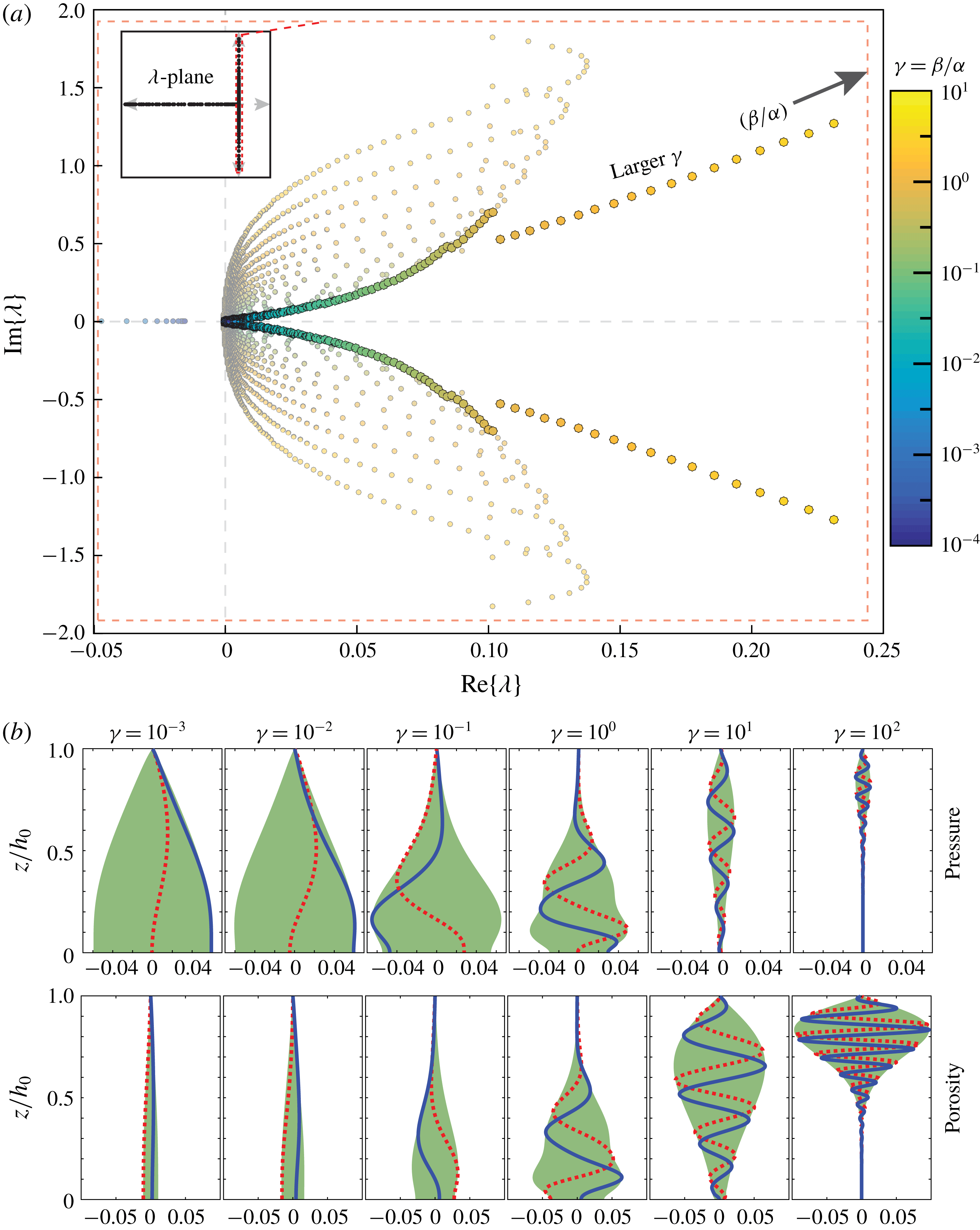
(a) Distribution of a subset of eigenvalues (growth parameters) in the complex plane for
 $f_{a}=0.05,\unicode[STIX]{x1D719}_{a}=0.5$
. The colours represent different values of
 $\unicode[STIX]{x1D6FE}$
. The eigenvalue with largest real part at each value of
 $\unicode[STIX]{x1D6FE}$
is represented by a larger, brighter circle, corresponding to the dominant wave that will grow for that particular
 $\unicode[STIX]{x1D6FE}$
. Inset figure shows the distribution of all of the eigenvalues from which those in the main figure are subset. The approximate range of the inset figure is
 $-2500<\text{Re}\{\unicode[STIX]{x1D706}\}<1,-2<\text{Im}\{\unicode[STIX]{x1D706}\}<2$
. (b) Eigenfunctions associated with the dominant eigenvalues over six values of
 $\unicode[STIX]{x1D6FE}$
showing the real part (blue, solid), imaginary part (red, dotted) and the region bounded by the modulus (green).

3.2.3 Distribution and variation of eigenvalues and eigenfunctions
For a given set of free parameters in the eigenvalue problem
 $(\unicode[STIX]{x1D6FE},f_{a},\unicode[STIX]{x1D719}_{a})$
, the eigenvalues (
 $\unicode[STIX]{x1D706}_{j}\in \mathbb{C}$
) are mainly distributed along the negative half –
 $\text{Re}\{\unicode[STIX]{x1D706}\}$
line; however, a small fraction have non-zero imaginary part (
 $\text{Im}\{\unicode[STIX]{x1D706}_{j}\}\neq 0$
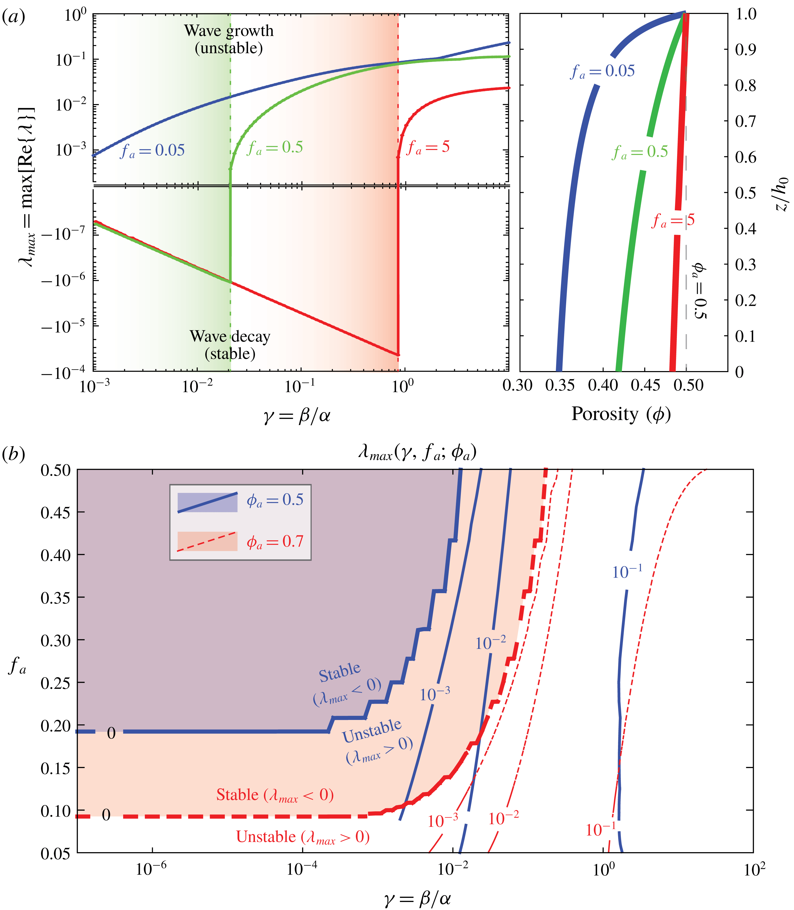
) and are near the stability–instability threshold (figure 3). For some ranges of the parameters, there exists eigenvalues with
 $\text{Re}\{\unicode[STIX]{x1D706}_{j}\}>0$
. Focusing on these positive eigenvalues, for a given value of
 $\unicode[STIX]{x1D6FE}$
, they are distributed in two symmetric branches (in the upper and lower half-planes) each of which generally begin near the origin and increase in imaginary and real parts (figure 3
a). In many cases, there is one eigenvalue on each branch with
 $\text{Re}\{\unicode[STIX]{x1D706}_{j}\}$
significantly larger than nearby eigenvalues. This larger positive eigenvalue corresponds to a dominating growth rate of its associated eigenfunction wave profiles. Because of this, these scenarios represent unstable flow regimes, causing particular excited oscillation to grow with time.
Varying the ratio of expansion rate to diffusion rate (
 $\unicode[STIX]{x1D6FE}$
) and examining the eigenvalues with largest real parts (
 $\unicode[STIX]{x1D706}_{max}$
), it is clear that
 $\unicode[STIX]{x1D706}_{max}(\unicode[STIX]{x1D6FE})$
increases with
 $\unicode[STIX]{x1D6FE}$
, meaning that for greater expansion and contraction and lesser diffusion, waves grow more quickly and the instability is stronger (figure 3). Stated in terms of physical parameters, less viscous or less permeable lavas allow greater wave growth than more viscous or permeable lavas. Where permeability is relatively low, pressure anomalies cannot relax sufficiently quickly by porous flow and as a consequence, the porosity will expand or contract as the pressure anomaly grows. Inversely, very permeable lavas allow efficient gas escape, smoothing out steep pressure gradients, limiting the growth of high and low pressure anomalies. Similarly, if the matrix viscosity is relatively low, even a small pressure anomaly will cause a significant change in porosity since over-pressurized regions are allowed to expand and under-pressurized regions allowed to contract against a weaker viscous resisting force in the matrix. These effects become self-reinforcing since the waves travel (
 $\text{Im}\{\unicode[STIX]{x1D706}\}\neq 0$
). In particular, the porosity governing equation predicts that a travelling pressure wave will induce a porosity wave that lags behind as it travels. As a result, the negative phase of a pressure wave lowers the porosity and permeability of the lava and the next arriving positive pressure wave phase will not diffuse through the low-permeability region easily, causing the pressure to rise behind the constriction, resulting in overall wave growth.
(a, left) The variation of
 $\unicode[STIX]{x1D706}_{max}(\unicode[STIX]{x1D6FE})$
for different values of
 $f_{a}$
showing the dependence of the stability–instability threshold on
 $\unicode[STIX]{x1D6FE}$
and (a, right) the associated steady-state porosity profile corresponding to each value of
 $f_{a}$
. (b) Contours of
 $\unicode[STIX]{x1D706}_{max}(\unicode[STIX]{x1D6FE},f_{a})$
for two values of
 $\unicode[STIX]{x1D719}_{a}$
showing the modification of the instability threshold (bold lines) with surface porosity.

The dominant eigenfunctions at each value of
 $\unicode[STIX]{x1D6FE}$
show that the maxima of the eigenfunction moduli or the location of the most principally excited waves gets closer to the surface for increasing
 $\unicode[STIX]{x1D6FE}$
(figure 3
b). Additionally, as
 $\unicode[STIX]{x1D6FE}$
increases, the pressure and porosity eigenfunctions have the same general shape; however, for the pressure, the maximum of the modulus decreases whereas for the porosity, the maximum increases, meaning that for larger
 $\unicode[STIX]{x1D6FE}$
, excited pressure waves are proportionally smaller in magnitude than their associated porosity waves. The structure of these eigenfunctions shows that the number of waves in the domain also increases, that is, the mean wavelength of the excited waves decreases with increasing
 $\unicode[STIX]{x1D6FE}$
. This trend corresponds with the notion that for small
 $\unicode[STIX]{x1D6FE}$
, the system is diffusion dominated, resulting in larger wavelengths and smoother gradients; however, for larger
 $\unicode[STIX]{x1D6FE}$
, the system experiences very little diffusion and so high frequency waves are allowed to grow. This instability is not universal for all values of
 $f_{a}$
and
 $\unicode[STIX]{x1D719}_{a}$
. For increasing values of
 $f_{a}$
and smaller
 $\unicode[STIX]{x1D6FE}$
,
 $\text{Re}\{\unicode[STIX]{x1D706}_{max}\}$
decreases until all even the largest eigenvalue becomes negative, implying linear stability of the steady state for those parameters (figure 4
a). For each set of stable
 $f_{a}$
and
 $\unicode[STIX]{x1D719}_{a}$
, there are stable and unstable values of
 $\unicode[STIX]{x1D6FE}$
. The critical value at which this threshold occurs (
 $\unicode[STIX]{x1D6FE}_{c}$
) increases with both
 $f_{a}$
and
 $\unicode[STIX]{x1D719}_{a}$
(figure 4
b). The complexity of this bifurcation contrasts with the unconditional stability predicted from the assumption of a uniform background state. An important consideration is the fact that as
 $f_{a}$
increases, the pressure and porosity background states become more approximately uniform and linear stability is predicted over a wider range of
 $\unicode[STIX]{x1D6FE}$
(figure 4
b). This mirrors the conditions of the LSA for a uniform background and agrees with that analysis. Critically, when
 $f_{a}$
is small, significant gradients form in the steady-state porosity field resulting from gravitational compaction of the column (figure 4
b). When
 $f_{a}$
is large, the dome is short and there is less overburden on the base of the dome which experiences less gravitational compaction. From these considerations, it is clear that increased dome height causes the porous lava to compact more, creating larger gradients in the dome’s porosity, which in turn initiate instability onset. Although this generalized eigenvalue problem yields insight into the generation of fluid instabilities in this system, significant simplifications have been made in reducing the highly nonlinear governing equations to a linear form. Consequently, the LSA above does not provide insight into higher-order processes which may limit the initial wave growth nor does it yield any insight into the dynamics near the
 $\unicode[STIX]{x1D719}\rightarrow \unicode[STIX]{x1D719}_{c}^{+}$
limit. Building from these simple analyses, we will next solve the one-dimensional (1-D) system ((2.7a
) and (2.7b
)) numerically to study the nonlinear effects that follow from the linear wave growth analysed here and gain insight into general characteristics of solutions.
4 Numerical solution of governing equations
In order to extend the above analysis of small amplitude pressure and porosity waves to determine the behaviour of these waves as they grow, we solve the 1-D system numerically given physically realistic boundary and initial conditions and examine some characteristic features of the solutions. The goal of this effort is to observe the behaviour of the system after it has evolved out of the regime of small amplitude waves which were studied in the LSA. Boundary data for the problem are estimable due to the constant ambient pressure at the dome surface and the inference of a pulsing flux of gas from depth based on observations of short-period (
 ${\sim}100$
–1000 s) oscillations in system-scale degassing observed across a variety of volcanic systems including lava dome systems (e.g. Tamburello et al.
Reference Tamburello, Aiuppa, McGonigle, Allard, Cannata, Giudice, Kantzas and Pering2013; Hyman et al.
Reference Hyman, Bursik and Legorreta Paulin2018).
We numerically solve an initial-boundary value problem (IVBP) for (2.7a ) and (2.7b ) taking the steady-state pressure and porosity profiles as initial conditions and specifying boundary data for (2.7a ) only. The system to be solved may be stated:
 $$\begin{eqnarray}\displaystyle & \displaystyle \unicode[STIX]{x1D719}\,\unicode[STIX]{x2202}_{t}p=\unicode[STIX]{x1D6FC}\,\unicode[STIX]{x2202}_{z}F-\unicode[STIX]{x1D6FD}p(p-f) & \displaystyle\end{eqnarray}$$
 $$\begin{eqnarray}\displaystyle & \displaystyle \unicode[STIX]{x2202}_{t}\unicode[STIX]{x1D719}=\unicode[STIX]{x1D6FD}(1-\unicode[STIX]{x1D719})(p-f) & \displaystyle\end{eqnarray}$$
 $$\begin{eqnarray}\displaystyle & \displaystyle p(z,0)=f(z) & \displaystyle\end{eqnarray}$$
 $$\begin{eqnarray}\displaystyle & \displaystyle \unicode[STIX]{x1D719}(z,0)=\unicode[STIX]{x1D719}_{s}(z) & \displaystyle\end{eqnarray}$$
 $$\begin{eqnarray}\displaystyle & \displaystyle F(0,t)=-\unicode[STIX]{x1D6EC}_{s}Q(t) & \displaystyle\end{eqnarray}$$
 $$\begin{eqnarray}\displaystyle & \displaystyle p(1,t)=f_{a}, & \displaystyle\end{eqnarray}$$
 $F=K(\unicode[STIX]{x1D719})p\,\unicode[STIX]{x2202}_{z}p$
,
 $\unicode[STIX]{x1D6EC}_{s}$
is the steady-state flux and
 $Q(t)$
is the temporal behaviour of gas flux into the dome base. To test the response of the dome pressure and porosity to oscillatory gas supply, we consider the dimensionless function
 $$\begin{eqnarray}\displaystyle Q(t)=1+q\sin (2\unicode[STIX]{x03C0}t) & & \displaystyle\end{eqnarray}$$
in which there is one oscillation of relative amplitude
 $q$
per dimensionless time unit, that is, time for the solution is measured in the number of flux oscillations elapsed. This included boundary flux is intended to incorporate the oscillatory degassing flux observed at many volcanic systems including dome systems (Holland et al.
Reference Holland, Watson, Phillips, Caricchi and Dalton2011; Girona et al.
Reference Girona, Costa, Taisne, Aggangan and Ildefonso2015; Hyman et al.
Reference Hyman, Bursik and Legorreta Paulin2018). Although an unstable (
 $f_{a},\unicode[STIX]{x1D719}_{a}$
) pair would produce instability without an added boundary flux, in nature the instability is initiated in a gas flow setting that includes these
 $O(\unicode[STIX]{x1D716})$
to
 $O(1)$
oscillations. Consequently the boundary flux data are included in a simplified manner – unimodal oscillations – to capture the basic aspects of this reality.
4.1 Finite-difference scheme
In solving this system numerically, we employ a modified backward Euler finite-difference (BEFD) scheme based on the well-established methods of Huyakorn & Pinder (Reference Huyakorn and Pinder1983) for modelling multiphase subsurface flow problems. To solve the coupled equations for pressure and porosity, equations (4.1a
) and (4.1b
) are discretized on a staggered, uniform grid where the pressures are located at the nodes (
 $z=j\unicode[STIX]{x0394}z$
) and the porosity and fluxes evaluated between the nodes (
 $z=(j\pm 1/2)\unicode[STIX]{x0394}z$
) on the interval
 $z\in [0,1]=\unicode[STIX]{x0394}z\{1,\ldots ,J\}$
. This approach respects the fact that variables like permeability and porosity control the flux of gas through the dome and thus should be located between nodes. Consequently, all pressure terms in the porosity equation are necessarily averaged between the two nearest nodes to the porosity half-node sites. For the pressure equation, since the flux is evaluated at the half-nodes, the pressure in the flux is similarly averaged. This local averaging in the numerical scheme can be thought of as a local volume element averaging as in Whitaker (Reference Whitaker1999). Using the staggered grid and local volume element averaging ensures that in simulating of the steady-state conditions, the diffusivity in the pressure equation (
 $K(\unicode[STIX]{x1D719})p$
) remains constant and reproduces the steady state upon updating.
The main modifications to the BEFD scheme is that the compaction terms are evolved according to forward differencing and the time steps are dynamic and are performed with a mid-time predictor–corrector step. The dynamic time stepping is based on the Jacobian of the compaction term in (4.1a ) at the last time step, that is
 $$\begin{eqnarray}\displaystyle t^{n+1}-t^{n}=\unicode[STIX]{x0394}t^{n+1}=0.1\left[\max _{j\in \{2,\ldots ,J-1\}}|(J_{p})_{j}^{n}|\right]^{-1},\quad \text{where }(J_{p})_{j}^{n}=\unicode[STIX]{x1D6FD}\frac{f_{j}-2p_{j}^{n}}{\unicode[STIX]{x1D719}_{j}^{n}}. & & \displaystyle\end{eqnarray}$$
Due to the nonlinearity in the diffusion term, for numerical solution to be tractable, this scheme is partially linearized by evaluating the non-constant diffusivity (
 $K(\unicode[STIX]{x1D719})p$
) at the previous time step. In the discretization of (4.1a
), the derivatives of the fluxes are evaluated as the difference across the edges of the cells:
 $$\begin{eqnarray}\displaystyle & \displaystyle \langle \unicode[STIX]{x1D719}_{j+1/2}^{\ast }\rangle _{-}\frac{p_{j}^{n+1}-p_{j}^{n}}{\unicode[STIX]{x0394}t^{n+1}}=\frac{\unicode[STIX]{x1D6FC}}{\unicode[STIX]{x0394}z}(F_{j+1/2}^{n+1}-F_{j-1/2}^{n+1})-\unicode[STIX]{x1D6FD}p_{j}^{\ast }(p_{j}^{\ast }-f_{j}) & \displaystyle\end{eqnarray}$$
 $$\begin{eqnarray}\displaystyle & \displaystyle \frac{\unicode[STIX]{x1D719}_{j\pm 1/2}^{n+1}-\unicode[STIX]{x1D719}_{j\pm 1/2}^{n}}{\unicode[STIX]{x0394}t^{n+1}}=\unicode[STIX]{x1D6FD}(1-\unicode[STIX]{x1D719}_{j\pm 1/2}^{\ast })\langle p_{j}^{\ast }-f_{j}\rangle _{\pm }, & \displaystyle\end{eqnarray}$$
 $$\begin{eqnarray}\displaystyle F_{j\pm 1/2}^{n+1}=K_{j\pm 1/2}^{\ast }\langle p_{j}^{\ast }\rangle _{\pm }\left(\pm \frac{p_{j\pm 1}^{n+1}-p_{j}^{n+1}}{\unicode[STIX]{x0394}z}\right) & & \displaystyle\end{eqnarray}$$
and the local volume averages are
 $\langle (\cdot )_{j}\rangle _{\pm }=1/2[(\cdot )_{j}+(\cdot )_{j\pm 1}]$
, centred at
 $z=(j\pm 1/2)\unicode[STIX]{x0394}z$
. Boundary values for (4.4a
) are discretized as
 $$\begin{eqnarray}\displaystyle & \displaystyle \frac{p_{2}^{n+1}-p_{1}^{n+1}}{\unicode[STIX]{x0394}z}=-\frac{\unicode[STIX]{x1D6EC}_{s}}{K_{1+1/2}^{\ast }\langle p_{1}^{\ast }\rangle _{+}}[1+q\sin (2\unicode[STIX]{x03C0}t^{n+1})] & \displaystyle\end{eqnarray}$$
 $$\begin{eqnarray}\displaystyle & \displaystyle p_{J}^{n+1}=f_{a}. & \displaystyle\end{eqnarray}$$
 $\ast =n$
(predictor at
 $n+1/2$
). In the second stage, the predicted values (
 $p_{j}^{n+1/2}$
and
 $\unicode[STIX]{x1D719}_{j\pm 1/2}^{n+1/2}$
) are substituted for the starred quantities and the equations are solved again for the full time step with updated estimates of the nonlinear coefficients (corrector).
4.2 Wave-diffusion behaviour
Solutions of (4.4a
) and (4.4b
) oscillate around the steady-state solutions
 $p_{s}(z)$
and
 $\unicode[STIX]{x1D719}_{s}(z)$
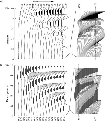
in a series of diffusive waves propagating toward the surface. As pressure waves pass, there are concordant porosity waves that lag just behind the pressure pulses (figure 5). Early in simulations, waves grow in a manner similar to the eigenfunctions of the LSA above; however, if the solution is continued, these waves grow and steepen as they propagate toward the surface (figure 5). This is an indication that nonlinear processes in the diffusion term of the pressure equation are dominating the simple linear wave growth predicted by the LSA. In general, the propagating pressure waves are steepest in the deepest troughs of the porosity waves. The amplitude of these waves continues to grow until
 $\unicode[STIX]{x1D719}=\unicode[STIX]{x1D719}_{c}$
, where the next arriving pressure wave steepens into a discontinuity (shock) (figure 5). In the regions of
 $\unicode[STIX]{x1D719}\leqslant \unicode[STIX]{x1D719}_{c}$
, the pressure and porosity evolve as predicted by (2.11), with the pressure increasing asymptotically back to the local magmastatic pressure (
 $f(z)$
) from
 $p=p_{c}(z)$
. Once multiple shocks develop, the excess pressure (
 $p-f$
) takes the form of a series of ‘N-waves’ separated by regions of magmastatic pressure in which
 $\unicode[STIX]{x1D719}<\unicode[STIX]{x1D719}_{c}$
(figure 5). The shocks generally slow and decay slightly as they propagate to shallower levels in the domain. Because the N-waves are separated by regions which are impermeable, there is no flow from one shock-bounded region to the next. Although no systematic study of the Rankine–Hugoniot relations for shock propagation speed has been made here owing to the complexity of the flux term, it is noted that in the simulations, successive N-waves rarely interact. These rare interactions always result in the up-gradient N-wave quickly diffusing into the down-gradient N-wave as the impermeable region separating the converging shocks becomes narrower until it vanishes (figure 5
a,b (right panels)). This behaviour is merely a consequence of the sudden hydraulic connection of two isolated permeable domains with different mean pressures. Although shock development is common across a wide set of free parameters in the problem, this wave behaviour is not universal. Still, in cases without shock development, waves steepen as they propagate toward the atmospheric boundary.
Numerical solution
 $(f_{a}=0.05,\unicode[STIX]{x1D719}_{a}=0.5,\unicode[STIX]{x1D6FC}=\unicode[STIX]{x1D6FD}=10,q=0.1)$
showing wave propagation, steepening and shock formation for porosity (a) and pressure (b) profiles. (a, left) Dashed lines on first and last porosity profiles represent steady-state porosity, the dotted line on first profile represents the percolation threshold
 $\unicode[STIX]{x1D719}_{c}$
, and the black regions represent the areas with
 $\unicode[STIX]{x1D719}<\unicode[STIX]{x1D719}_{c}$
. (b, left) Light and dark grey shaded regions represent positive and negative pressure anomalies respectively. (a, right) and (b, right) show the behaviour of the porosity and pressure respectively late in the simulation during an interaction of two shocks between
 $0\leqslant z/h_{0}\leqslant 0.25$
.

5 Lava dome survival experiment
Following from the study of wave growth in the LSA and the observation of nonlinear wave growth and development of shocks in the direct numerical simulation, we are interested in how these characteristics affect the pressurization and destruction of lava domes. Particularly, we are interested in the sudden explosion of lava domes undergoing the type of oscillatory degassing observed at many volcanoes. As mentioned above, to simulate the overall behaviour of a long period of lava dome extrusion and destruction cycles, the space of lava properties must be sampled widely, resulting in a set of
 $\unicode[STIX]{x1D6FC}$
and
 $\unicode[STIX]{x1D6FD}$
that vary over many orders of magnitude. Using the result of the LSA as a guide, we choose a representative pair of
 $f_{a}$
and
 $\unicode[STIX]{x1D719}_{a}$
(
 $f_{a}=0.05$
,
 $\unicode[STIX]{x1D719}_{a}=0.5$
) which initiate instability for a wide range of
 $\unicode[STIX]{x1D6FE}$
and sample
 $\unicode[STIX]{x1D6FC}$
and
 $\unicode[STIX]{x1D6FD}$
to test how long the given sample will survive until fragmentation. To assess this, a fragmentation criterion must be established.
5.1 Porosity-dependent fragmentation threshold
From experimental studies of lava fragmentation, Spieler et al. (Reference Spieler, Kennedy, Kueppers, Dingwell, Scheu and Taddeucci2004) determined an empirical fragmentation threshold relationship that relates the pressure difference required to fragment a sample (
 $\unicode[STIX]{x0394}p$
) to the sample porosity as
 $$\begin{eqnarray}\displaystyle \unicode[STIX]{x0394}p=\frac{\unicode[STIX]{x1D70E}_{m}}{\unicode[STIX]{x1D719}}, & & \displaystyle\end{eqnarray}$$
where
 $\unicode[STIX]{x1D70E}_{m}$
is taken as 1 MPa, which they noted should not be expected to hold for highly porous rocks. This relationship is an alternative to earlier studies which had concluded that porosity was the main control on fragmentation, considering fragmentation thresholds of porosities between 65 and 85 % (Sparks Reference Sparks1978; Sparks et al.
Reference Sparks, Barclay, Jaupart, Mader and Phillips1994). As a result we modify the threshold of Spieler et al. (Reference Spieler, Kennedy, Kueppers, Dingwell, Scheu and Taddeucci2004) to respect the failure of this relationship for large porosity:
 $$\begin{eqnarray}\displaystyle \unicode[STIX]{x0394}p(\unicode[STIX]{x1D719})=\left\{\begin{array}{@{}ll@{}}\displaystyle \frac{1~\text{MPa}}{\unicode[STIX]{x1D719}}\quad & \unicode[STIX]{x1D719}<0.8\\ 0\quad & \unicode[STIX]{x1D719}\geqslant 0.8.\end{array}\right. & & \displaystyle\end{eqnarray}$$
We incorporate this threshold into the numerical model presented above by predicting failure at time
 $t_{f}=t^{n+1}$
if
 $$\begin{eqnarray}\displaystyle p_{j}^{n+1}-f_{j}\geqslant \unicode[STIX]{x0394}p(\langle \unicode[STIX]{x1D719}_{j+1/2}^{n+1}\rangle _{-}). & & \displaystyle\end{eqnarray}$$
In doing so, we can examine the predicted failure times across a range of representative parameters for intermediate-composition lava domes (table 1).
In the development of the LSA, we showed that for initial wave growth, the diffusion rate parameter
 $\unicode[STIX]{x1D6FC}$
mainly scales time during wave growth whereas the ratio of expansion rate to diffusion rate (
 $\unicode[STIX]{x1D6FE}$
) controls the behaviour of these waves. In the nonlinear case,
 $\unicode[STIX]{x1D6FC}$
is expected to not only scale time, but also control some nonlinear effects due to the severe nonlinearity of the diffusion in (2.7a
) and so
 $\unicode[STIX]{x1D6FC}$
and
 $\unicode[STIX]{x1D6FD}$
are varied independently in the ranges
 $0\leqslant \log (\unicode[STIX]{x1D6FC})\leqslant 4$
and
 $-1\leqslant \log (\unicode[STIX]{x1D6FD})\leqslant 2$
. Additionally, the boundary flux oscillation strength is varied in the range
 $0.1\leqslant q\leqslant 1$
. As a result, we consider the failure time as a function of the three-dimensional sample space:
 $t_{f}:S\subset \mathbb{R}^{3}\rightarrow \mathbb{R}$
.
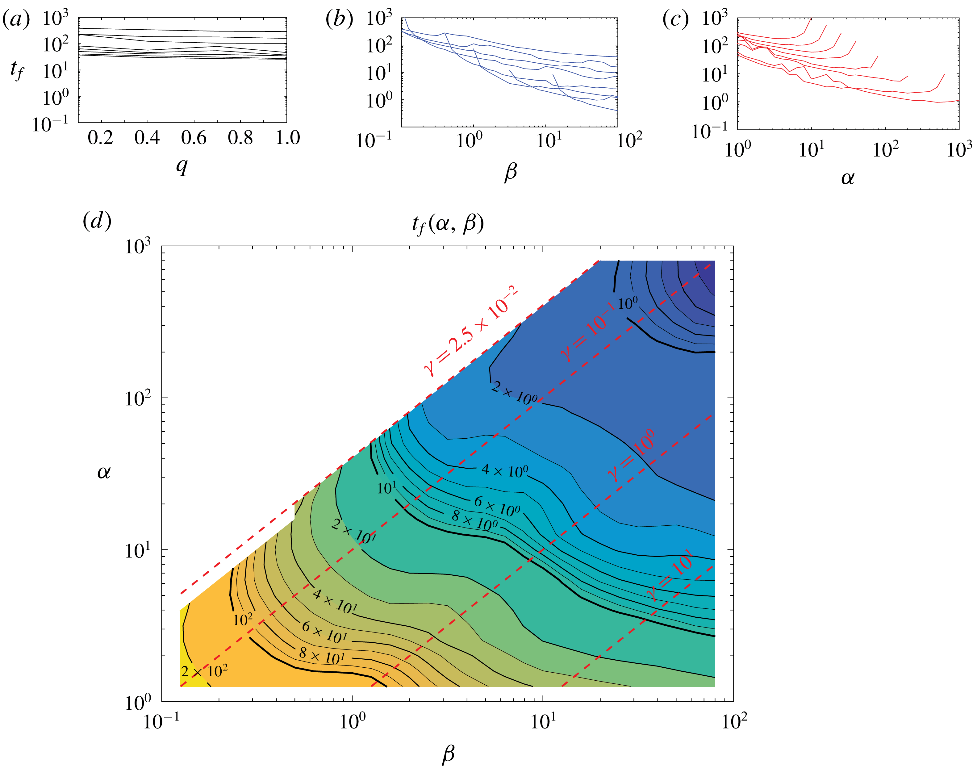
(a–c) The variation of
 $t_{f}$
with
 $\unicode[STIX]{x1D6FC}$
,
 $\unicode[STIX]{x1D6FD}$
and
 $q$
for several values of the other two parameters. (d) Logarithmic contour plot of
 $t_{f}(\unicode[STIX]{x1D6FC},\unicode[STIX]{x1D6FD})$
generated by averaging values of
 $t_{f}(\unicode[STIX]{x1D6FC},\unicode[STIX]{x1D6FD},q)$
through
 $q$
and a single convolution with a
 $3\times 3$
running average filter. Red dotted contours represent values of
 $\unicode[STIX]{x1D6FE}$
.

5.2 Parametric dependence of dome failure times
As anticipated by the derivation of the LSA, the diffusion rate parameter
 $\unicode[STIX]{x1D6FC}$
has the strongest control on the failure time followed by the compaction rate parameter
 $\unicode[STIX]{x1D6FD}$
and relative boundary oscillation amplitude
 $q$
. Although
 $q\neq 0$
is the only condition generating the non-equilibrium conditions, variation of
 $q$
explains almost none of the variability in computed survival times (
 $t_{f}$
) compared with
 $\unicode[STIX]{x1D6FC}$
and
 $\unicode[STIX]{x1D6FD}$
(figure 6
a–c). For example, the full domain of
 $q$
is only able to change
 $t_{f}(q)$
by less than one order of magnitude (figure 6
a) compared with
 ${\sim}2$
orders of magnitude for
 $\unicode[STIX]{x1D6FD}$
(figure 6
b) and
 $1-2$
orders of magnitude for
 $\unicode[STIX]{x1D6FC}$
(figure 6
c). Because of this, we principally analyse the variation of
 $t_{f}$
through the parameter space of
 $\{\unicode[STIX]{x1D6FC}\}\times \{\unicode[STIX]{x1D6FD}\}$
only, averaging
 $t_{f}$
through the full space along
 $q$
(figure 6
d). The computed function
 $t_{f}(\unicode[STIX]{x1D6FC},\unicode[STIX]{x1D6FD})$
is only defined on a subset of the parameter space approximately where
 $\unicode[STIX]{x1D6FE}\geqslant O(10^{-2})$
(figure 6
d). The excluded region includes parameter values for which initial instability causes wave growth as predicted by the LSA; however, higher order terms limit the growth and the pressure and porosity waves are bounded below the fragmentation threshold. Analysis of these solutions is beyond the scope of the present work. Within the domain of finite fragmentation times, increased
 $\unicode[STIX]{x1D6FD}$
decreases the survival time with an approximately exponential decay. By contrast, increasing
 $\unicode[STIX]{x1D6FC}$
decreases
 $t_{f}$
on approximately
 $\unicode[STIX]{x1D6FC}<10\unicode[STIX]{x1D6FD}$
; however, with higher
 $\unicode[STIX]{x1D6FC}$
, the survival time grows quickly until it meets the undefined region in which the higher-order effects prevent fragmentation. Although the value of
 $\unicode[STIX]{x1D6FE}$
plays a large role in the initial wave growth and in the behaviour of the excited waves, it does not seem to exert a strong control over the timing of failure by itself.
6 Discussion
6.1 Transition between stability and instability
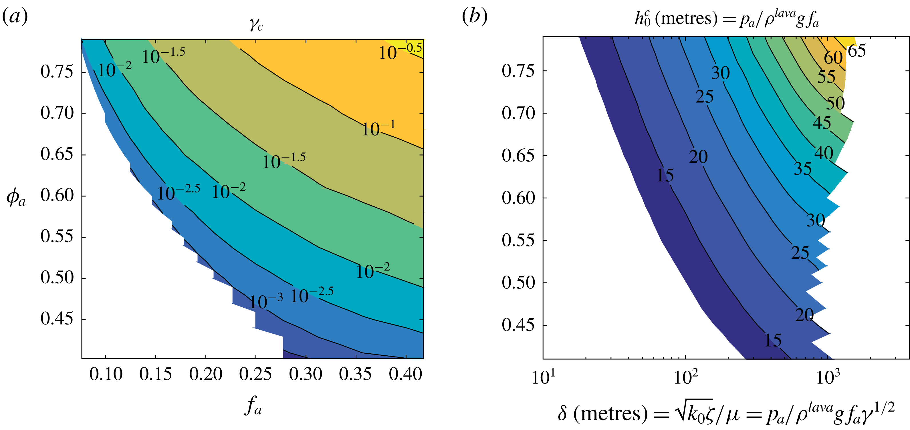
(a) Non-dimensional and (b) dimensional contour plots of the threshold functions (a)
 $\unicode[STIX]{x1D6FE}_{c}(f_{a},\unicode[STIX]{x1D719}_{a})$
and (b)
 $h_{0}^{c}(\unicode[STIX]{x1D6FF},\unicode[STIX]{x1D719}_{a})$
showing the threshold for stability versus instability. (a) Values of
 $\unicode[STIX]{x1D6FE}$
larger than
 $\unicode[STIX]{x1D6FE}_{c}(f_{a},\unicode[STIX]{x1D719}_{a})$
yield instability. (b) Values of
 $h_{0}$
larger than
 $h_{0}^{c}(\unicode[STIX]{x1D6FF},\unicode[STIX]{x1D719}_{a})$
yield instability. White space indicates regions without data coverage.

From the numerical LSA for non-constant background conditions, it is clear that varying the dome height and the surface porosity causes growth rates to transition from stable
 $\text{Re}\{\unicode[STIX]{x1D706}_{max}\}<0$
to unstable
 $\text{Re}\{\unicode[STIX]{x1D706}_{max}\}>0$
for some critical value of the ratio of diffusion and compaction rates (
 $\unicode[STIX]{x1D6FE}_{c}$
). In determining the onset of instability, we are mainly interested in determining the relationships between the most uncertain or variable physical parameters:
 $k_{0}$
,
 $\unicode[STIX]{x1D701}$
,
 ${\dot{m}}_{s}$
,
 $T^{dome}$
,
 $A$
and
 $h_{0}$
. Because of the nonlinear transformation of these physical parameters into
 $\unicode[STIX]{x1D6FE}$
,
 $f_{a}$
and
 $\unicode[STIX]{x1D719}_{a}$
, which governing the underlying physics of instability onset, the effects of the different physical parameters cannot be fully decoupled. However, by fixing the values of the better constrained physical parameters
 $p_{a}$
,
 $\unicode[STIX]{x1D70C}^{lava}$
, and
 $g$
(table 1) and rewriting
 $h_{0}$
and
 $\unicode[STIX]{x1D6FF}$
in terms of
 $f_{a}$
,
 $\unicode[STIX]{x1D6FE}$
gives
 $$\begin{eqnarray}\displaystyle h_{0}=\frac{p_{a}}{\unicode[STIX]{x1D70C}^{lava}gf_{a}}\quad \text{and}\quad \unicode[STIX]{x1D6FF}=\sqrt{\frac{k_{0}\unicode[STIX]{x1D701}}{\unicode[STIX]{x1D707}}}=\frac{p_{a}}{\unicode[STIX]{x1D70C}^{lava}gf_{a}\sqrt{\unicode[STIX]{x1D6FE}}}. & & \displaystyle\end{eqnarray}$$
Consequently, the relationship between
 $f_{a}$
and the critical value of
 $\unicode[STIX]{x1D6FE}$
for instability onset can be mapped onto a similar relationship between the compaction length
 $\unicode[STIX]{x1D6FF}$
and the threshold value of dome thickness for instability onset (
 $h_{0}^{c}$
) (figure 7). The dome thickness required to trigger instability onset increases with both
 $\unicode[STIX]{x1D6FF}$
and
 $\unicode[STIX]{x1D719}_{a}$
(figure 7). This suggests that more permeable, more viscous lavas can support thicker domes before the onset of flow instability. Similarly, the critical dome thickness
 $h_{0}^{c}$
increases with surface porosity, which is related to higher mean gas flux (
 ${\dot{m}}_{s}/A$
, equation (2.13)).
Although the background pressure gradient is unchanged by variations in dome thickness or surface porosity, the porosity field is affected by the dome thickness and the surface porosity or gas flux. Increased dome thickness gives a smaller background porosity gradient and higher porosities throughout whereas increased
 $\unicode[STIX]{x1D719}_{a}$
increases the porosity gradient and values near the surface with very minor increases in porosity away from the surface. Because gas flow becomes unstable when domes cross a thickness threshold, the likelihood of flow instability grows the longer lava dome extrusion takes place. This in turn increases the likelihood of lava dome overpressurization and destruction.
Survival distribution for (a) lava dome volumes measured by (Gómez-Vazquez et al. Reference Gómez-Vazquez, De la Cruz-Reyna and Mendoza-Rosas2016) at Volcán Popocatépetl, Mexico and (b) time to fragmentation as computed for the model in this study.

6.2 Survival time distribution
To make an ensemble model of the above numerical experiment, the above parametric survival function
 $t_{f}(\unicode[STIX]{x1D6FC},\unicode[STIX]{x1D6FD})$
is sampled uniformly in
 $\log \unicode[STIX]{x1D6FC}$
and
 $\log \unicode[STIX]{x1D6FD}$
where parameters such as lava viscosity and permeability may vary over many orders of magnitude as could be reasonably expected in a volcanic system like Popocatépetl. The distribution of survival times generated by the numerical experiment show a significant decrease in frequency with survival time (figure 8
b). The number of domes surviving longer than a given time – the survival distribution – can be modelled as a decaying exponential over different domains of the distribution (figure 8
b). In general, successive lava dome eruptions may be expected to extrude lavas with more uniform properties than were sampled here and as a result would be expected to show significantly less total dispersion in survival times. Because different exponentials fit different segments of the survival distribution, narrower parameter sampling would likely result in a distribution which conforms better to one particular exponential survival distribution. Although the numerical solutions generating this distribution were generated from a specific set of
 $f_{a}$
and
 $\unicode[STIX]{x1D719}_{a}$
, survival distributions constructed from different (
 $f_{a},\unicode[STIX]{x1D719}_{a}$
) pairs (figure 7
a) are expected to have similarities with the distribution shown in figure 8.
Because of the natural scaling of time to measure the number of boundary flux oscillations, the survival times record the number of such oscillations between when the dome grows to the thickness
 $h_{0}$
and when fragmentation begins. Although this is not a perfect representation of time since instability onset, we consider it a useful approximation. Consequently, the modelled survival times are expected to relate to the volume of lava extruded at the time of explosion because of the slow, approximately continuous growth of lava domes over the considered time scales. In this context, the basic characteristics of the survival time distribution generated here appears to compare favourably with the survival volume distribution measured at Popocatépetl, Mexico from 1996–2016 (figure 8
a) (Gómez-Vazquez et al.
Reference Gómez-Vazquez, De la Cruz-Reyna and Mendoza-Rosas2016). Because of the large uncertainty in extrusion rates, lava properties, and the fact that dome thicknesses at explosion were not consistent at Popocatépetl during this period, the theoretical survival distribution can only be compared to the natural data qualitatively. Despite this, the apparent agreement suggests that lava dome growth and explosion cycles may be governed by the dynamics of gas–lava VDPM flows described here and that despite the unpredictability of individual lava dome explosion cycles at similar volcanoes, the variation in survival volumes of lava domes is the product of random variation in the underlying parameters governing the flow such as the lava viscosity and permeability. Because the permeability coefficient used in the present study is related to the mean bubble radius (
 $r_{b}$
) by
 $k_{0}\approx 0.13\,r_{b}^{2}$
, some of the properties of these flows could be reconstructed from detailed study of bubble sizes in cooled lava dome remnants or the fragmental products of lava dome explosions.
7 Conclusions
(i) The pressure-driven flow of compressible pore fluids in viscously deformable porous media as applied to gas in lava domes is governed by nonlinear parabolic differential equations describing pressure and porosity diffusion and wave motion. In this formulation, equilibrium solutions exist which balance the pressure and porosity where increased equilibrium pressure compresses the medium, lowering the porosity. However, under non-steady conditions, positive pressure anomalies cause an increase in the porosity and permeability of the medium which in turn accelerates the flux of gas.
(ii) Linear stability analysis of the governing equations suggests that the flow of gas and lava is stable for very thin domes, but as a dome grows, a thickness threshold is exceeded and instability is generated causing the growth of pressure and porosity waves. This instability is principally caused by the increased gravitational compaction of the bulk medium due to the vertical nature of the problem and the compressibility of the pore fluid. Because of the gradients present in the equilibrium solutions, particularly that of the porosity, the growth of these waves is not uniform throughout the lava dome thickness and the distribution of growth constants in the complex plane is difficult to characterize. However, the onset of instability (
 $\unicode[STIX]{x1D706}_{max}>0$
) is governed both by properties of the equilibrium solution including the dome thickness
 $h_{0}$
, the surface porosity
 $\unicode[STIX]{x1D719}_{a}$
(a measure of the mean gas flux), and the compaction length, itself a measure of the permeability and viscosities of the lava dome and gas. In particular, less permeable, less viscous domes are more unstable for a given dome thickness than domes with higher permeability or lava viscosity since more efficient gas escape (higher permeability) and a more rigid medium (higher lava viscosity) hinder the growth of pressure and porosity waves.
(iii) In general, the flow of gas and lava approaches and eventually exceeds the critical thickness for instability as a particular lava dome grows over time. Above this height threshold, the steady flow of gas through the lava medium is unstable, producing growth of pressure and porosity waves which may cause pressurization-induced destruction of the lava dome. Because lava domes thicken over the duration of an eruption, the likelihood of instability onset and dome destruction increases over time, even without specific knowledge of the lava viscosity and permeability.
(iv) Direct numerical experimentation across a wide range of lava parameters confirms this inference from the study of linear stability, suggesting that pressure and porosity waves grow sufficiently large to cause fragmentation of the lava medium, which would in turn initiate dome destruction. Qualitative agreement between the distribution of survival times generated by random sampling in the numerical experiment with the natural dome volume survival distribution generated by Gómez-Vazquez et al. (Reference Gómez-Vazquez, De la Cruz-Reyna and Mendoza-Rosas2016) from lava dome extrusions at Volcán Popocatépetl, Mexico from 1996 to 2016 suggests that the dome thickening-induced instability may drive the cycles of lava dome growth and destruction at Popocatépetl and perhaps other lava dome-producing volcanoes.
Acknowledgements
The present work was funded by private donations to the University at Buffalo Foundation, NASA grant NNX12AQ10G, and by a Center for Geohazards Studies Student Research Award. The views expressed in the present contribution are those of the authors alone. We thank the Associate Editor and three anonymous reviewers for their help in improving the manuscript.