NOMENCLATURE
- LSB
laminar separation bubble
- L, R
discretised linear operators
- N
disturbance wave amplification factor
- q
vector of fluid variables
- PSE
parabolised stability equations
- p
pressure
- Stθ
Strouhal number based on the momentum thickness at separation
- x, y, z
streamwise, wall-normal, and spanwise co-ordinates
- u, v, w
streamwise, wall-normal, and spanwise velocity components
- u rev
peak reversed flow
Superscripts
- –
base flow
- '
fluctuation
- ̆
fourier mode
- ∼
PSE shape function
- ^
Eigenfunction
Greek symbol
- α
streamwise wavenumber
- β
spanwise wavenumber
- βc
critical spanwise wavenumber for the primary instability
 $${\rm \bar{\rdelta }}_{{{\rm max}}} $$
peak displacement thickness in boundary-layer units
- φ
obliqueness angle of waves with respect to the x-axis
- λx
streamwise wavelength
- λz
spanwise wavelength
- μ
transformed eigenvalue
- σ
shift parameter
- θs
momentum thickness at separation
- ω
circular frequency
- ωz
spanwise vorticity
- Ω
cross-stream computational domain

1.0 INTRODUCTION
The formation of laminar separation bubbles (LSBs) is an usual phenomenon on aerodynamic surfaces that takes place when strong enough adverse-pressure-gradients are present. They are associated with a potentially severe detrimental impact on the lift, drag and pitching momentum, reason that has motivated continuous research since the works of Gault(Reference Gault1) and McCullough and Gault(Reference McCullough and Gault2). The characteristics of the flow after separation, the eventual reattachment and its effect on the aerodynamics are governed primarily by the laminar-turbulent transition process and the details of the flow instabilities triggering it.
Laminar separation bubbles have the potential to amplify external disturbances in a dramatic manner: the orders-of-magnitude amplitude growth resulting from convective instability mechanisms typically leads to strong non-linear phenomena and transition to turbulence even at low excitation levels(Reference Alam and Sandham3–Reference Marxen, Lang and Rist6). Most works agree that the fundamental mechanism is the amplification of Tollmien–Schlichting (T–S) waves pre-existing within the boundary-layer upstream of the separation, by the inflectional instability within the separated shear layer. Spanwise vortices are then formed and shed. Some researchers investigated the origin of three-dimensionality under these circumstances, attributing it to secondary instabilities of the spanwise vortices(Reference Marxen, Lang and Rist6, Reference Rist and Maucher7). On the other hand, Rist and Maucher(Reference Rist and Maucher8) investigated the non-linear interactions occurring when two oblique T–S waves were excited, finding that the transition occurred in an abrupt manner (which they termed oblique breakdown) more similar to the experimental observations of unforced LSBs, than under other forcing conditions in which the dominant component was 2D and very coherent spanwise vortices were realised.
The prominent amplifier behaviour manifested by LSBs does not suffice, however, to explain the very rich and involved physics observed both in experiments and numerical simulations, suggesting that other instability mechanisms must be at play. In this context, Rodríguez et al.(Reference Rodríguez, Gennaro and Juniper9) considered theoretically the instability of LSBs in the absence of externally imposed disturbances. It was demonstrated that a 3D global instability of centrifugal nature, first found by Theofilis et al.(Reference Theofilis, Hein and Dallmann10) becomes active for LSBs that are significantly weaker than required for the onset of self-sustained two-dimensional oscillations. The strength of the LSBs was quantified using the percentage of the peak reversed flow over the free-stream velocity, u rev, and it was shown that u rev∼7–8% was enough for 3D instability to set in. This value contrasts with the generally accepted threshold for the self-sustain oscillator, which requires u rev∼16–20%(Reference Alam and Sandham3, Reference Rist and Maucher7). As a consequence of the centrifugal instability, LSBs develop a spanwise modulation of their properties (recirculation, streamwise and wall-normal extent). The ensuing non-linear evolution leads to the saturation of this primary centrifugal instability and results in fully three-dimensional flow fields(Reference Rodríguez, Gennaro and Souza11, Reference Rodríguez and Theofilis12).
This paper considers the possible situation in which the two instability mechanisms, namely the self-excited centrifugal instability and the convective amplification of disturbance waves originated upstream in the boundary layer, co-exist. The spanwise velocity gradients associated with the centrifugal instability increase remarkably the peak recirculation at some locations and introduce cross-plane shear components, which is known to have the potential to enhance the inviscid instability of the separated shear layer(Reference Kawahara, Jimémez, Uhlmann and Pinelli13, Reference Saxena, Leibovich and Berkooz14). Additionally, the LSB three-dimensionality can distort the disturbance waves by introducing streamwise vorticity, replacing the formation of spanwise vortices by more involved three-dimensional vortical structures. In this respect, it is worth noting that experimental and numerical studies observed the spontaneous appearance of stationary streamwise streaks(Reference Spalart and Strelets15, Reference Watmuff16) or three-dimensionality(Reference Diwan and Ramesh4) underlying the dominant convective instability and without explicitly imposing them. Incidentally, recent experimental visualisations using particle image velocimetry reported the formation and shedding of spanwise-modulated vortices from separation bubbles without the application of any explicit forcing.
The rest of the paper is organised as follows. Section 2 recapitulates the precedent studies on the self-excited instability and describes the resulting steady three-dimensional LSBs. These flow fields will be subject to linear stability analysis in the subsequent sections. An extension of the parabolised stability equations (PSE), sometimes referred to as 3D-PSE(Reference Broadhurst and Sherwin17, Reference Herbert18), that considers three-dimensional base flows with a strong dependence on the cross-stream plane and slowly divergent on the streamwise direction, is described in Section 3. Subsequently 3D-PSE is used to study the linear amplification of initially plane T–S waves by the LSBs. The results of the analyses are described in Section 4. Finally, some concluding remarks are given in Section 5.
2.0 THREE-DIMENSIONAL LAMINAR SEPARATION BUBBLES RESULTING FROM THE SELF-EXCITED PRIMARY INSTABILITY
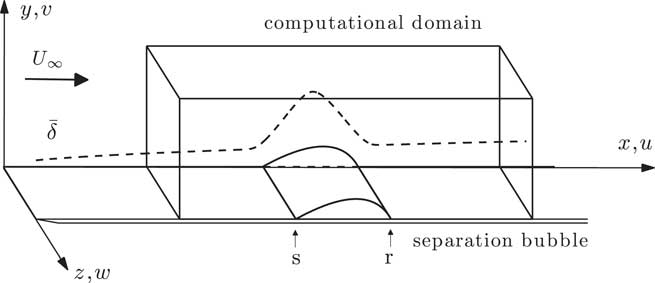
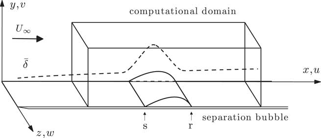
Figure 1 illustrates the problem geometry. The streamwise, wall-normal and spanwise co-ordinates are denoted by x, y and z, respectively, and the corresponding velocity components by u, v and w. Following our previous works(Reference Rodríguez, Gennaro and Juniper9, Reference Rodríguez, Gennaro and Souza11, Reference Rodríguez and Theofilis12), a family of LSBs on a flat-plate boundary layer is considered. Baseline LSBs are computed using an inverse non-similar boundary-layer formulation in which a streamwise distribution of the displacement thickness is prescribed, circumventing Goldstein’s singularity and allowing for the recovery of separated flows. For a bounded streamwise extent, the displacement thickness is smoothly increased over the corresponding value for a zero-pressure-gradient boundary layer. The streamwise extent of the displacement thickness increase is fixed, and different decelerated flows are computed by varying the peak displacement thickness  $${\rm \bar{\rdelta }}_{{{\rm max}}} $$. Fully laminar, two-dimensional and steady flows with a closed recirculation region are computed in this manner, and are subject to analysis and denoted by q0=(u 0, v0, 0, p 0)T in what follows. The main characteristics of these baseline LSBs make them comparable to other LSBs reported in the literature: the Reynolds number based on free-stream velocity and length of the separated region is ReL=37,000–40,500; the Reynolds number based on momentum thickness and free-stream velocity at the separation location is
 $${\rm Re}_{{{\rm \rtheta }_{{\rm s}} }} {\equals}208{\minus}212$$; and the peak reversed flow u 0,rev=5–12%.
Problem geometry and computational domain.
The dimensionless form used in this work is defined with the free-stream velocity at the inlet section. The boundary-layer displacement thickness at a location upstream of the deceleration, where the flow corresponds to a zero-pressure-gradient, is used to scale distances. The Reynolds number based on this displacement thickness is 450, and the corresponding streamwise co-ordinate is x=152. This choice of non-dimensionalisation is done to ease the computations, as it remains the same for all the baseline LSBs.
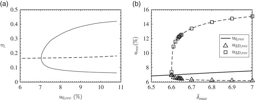
Global eigenmode analyses, considering modal perturbations of the form  $$\widehat{{\bf q}}(x,y)\,\exp [\:i\,\:({\rm \rbeta }z{\minus}{\rm \romega }t)]$$, show that the three-dimensional centrifugal instability is the only self-excited linear mechanism active in the present baseline LSBs. Figure 2(a) shows the neutral curve (solid line) and the dominant spanwise wavenumber β (dashed line) as a function of u 0, rev. The main characteristics of this instability are (i) its frequency ω=0; (ii) it is not active for two-dimensional perturbations; (iii) it has a preferential wavenumber βc≈0.166 for the present LSBs, corresponding to a spanwise wavenumber λz/θs≈76, where θs is the momentum thickness at separation and λz=2π/βc; and (iv) it becomes active for reversed flow larger than u 0,rev≈6.98% (
 $${\rm \bar{\rdelta }}_{{{\rm max}}} \,\approx\,6.6$$). Detailed information on the primary instability analyses can be found elsewhere(Reference Rodríguez, Gennaro and Juniper9).
(a) Neutral curve for the primary instability eigenmode (solid line) and spanwise wavenumber of maximum growth rate (dashed line). (b) Bifurcation diagram of the primary instability, corresponding to the saturation of the three-dimensional instability. Peak reversed flow of the baseline LSB (u 0,rev, solid line without symbols), the saturated three-dimensional flow (u 3D,rev, squares) and the spanwise-averaged saturated flow (u 2D,rev, circles).
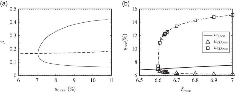
Rodríguez et al(Reference Rodríguez, Gennaro and Souza11). studied the non-linear evolution subsequent to the onset of the three-dimensional instability using direct numerical simulations, and determined that it corresponds to a supercritical pitchfork bifurcation: the non-linear interactions involving the fundamental wavenumber βc, its harmonics and the “mean flow distortion” (in this case the spanwise-uniform component β=0) result in the saturation of the disturbance growth and the formation of fully three-dimensional yet steady flows. The three-dimensional flows at saturated conditions are denoted by q3D in what follows, while q2D refers to their spanwise average. Figure 2(b) shows the bifurcation diagram: the peak reversed flow in the undisturbed baseline LSB u 0,rev, the three-dimensional saturated flow u 3D,rev and its spanwise average u 2D,rev, as a function of the peak displacement thickness in boundary-layer units,  $${\rm \bar{\rdelta }}_{{{\rm max}}} $$. While the centrifugal instability reduces the mean bubble recirculation, the spanwise modulation of the separated shear layer results in localised peak reversed flow greater than u 3D,rev=10%. As shown by Saxena et al.(Reference Saxena, Leibovich and Berkooz14) and Kawahara et al.(Reference Kawahara, Jimémez, Uhlmann and Pinelli13), the spanwise modulation of shear layers can enhance the inviscid Kelvin–Helmholtz instability mechanism. This is of particular interest to the LSBs, because it can impact the convective amplification of T–S waves within the boundary layer as they travel through the separated shear layer.
3.0 METHODOLOGY
3.1 Three-dimensional PSEs
The total flow field is separated into a time-independent base flow and temporal fluctuations q(x,t)= $${\bf \bar{q}}$$(x)+q′(x,t), where x=(x,y,z)T is the vector of co-ordinates in a Cartesian reference system, t is the time and q=(u,v,w,p)T is a vector comprising the velocity components and pressure p. The time-independence of the base flow allows for the introduction of Fourier modes for the circular frequency ω, as
 $${\bf q'}({\bf x},t){\equals}\mathop{\sum}\limits_{\rm \romega } {\bf \mathord{\buildrel{\lower3pt\hbox{$\scriptscriptstyle\smile$}}\over q} }_{{\rm \romega }} ({\bf x})\:e\:^{{{\minus}\:{\bf i}{\rm \romega }t}} {\plus}c.c$$
where c.c. stands for the complex conjugate.
Based on the multiple-scales approach and originally devised for the study of Tollmien–Schlichting waves on transitional boundary layers, PSE accounts for a slow divergence of the mean flow properties and has been shown to deliver results comparable to direct numerical simulations for convectively unstable laminar and transitional flows(Reference Bertolotti, Herbert and Spalart19, Reference Chang, Malik, Erlenbacher and Hussaini20). The fluctuations  $${\bf \mathord{\buildrel{\lower3pt\hbox{$\scriptscriptstyle\smile$}}\over q} }_{\romega } \left( {\bf x} \right)$$ are decomposed into a shape function
 $${\bf \mathord{\buildrel{\lower3pt\hbox{$\scriptscriptstyle\smile$}}\over q} }_{\romega } $$, which is also slowly varying along the streamwise direction x, and a rapidly varying wave-like part
 $${\bf \mathord{\buildrel{\lower3pt\hbox{$\scriptscriptstyle\smile$}}\over q} }_{{\rm \romega }} {\equals}A_{{\rm \romega }} (x)\,{\tilde {\bf q}}_{{\rm \romega }} (x,y,z){\equals}A_{{\rm \romega }} (x_{0} )\,{\rm exp}\left( {\:i\:{\int}_{x_{0} }^x \ralpha _{{\rm \romega }} ({\rm \rxi })\:d\:{\rm \rxi }} \right){\tilde {\bf q}}_{{\rm \romega }} (x,y,z)$$
The complex quantity αω=αr+iαi is a streamwise wavenumber, for which a slow variation with x is assumed as well. The streamwise co-ordinate x 0 is the location where the PSE integration is initialised. Upon substitution of (2) in the linearised incompressible Navier–Stokes and continuity equations, and neglecting terms involving second-order derivatives of the fluctuations on x, one arrives at the system of equations
 $${\bf L}{{\partial {\tilde {\bf q}}_{{\rm \romega }} } \over {\partial x}}{\equals}{R\tilde{\bf q}}_{{\rm \romega }} ,...$$
where the linear operators L and R depend on the mean flow quantities and their first spatial derivatives, wavenumber α, frequency ω, Reynolds number Re and spatial differentiation operators on the cross-stream directions:  $${\cal D}_{y} ,{\cal D}_{z} ,{\cal D}_{{yy}} $$, and
 $${\cal D}_{{zz}} $$.
The decomposition (2) and the governing equations (3) do not define uniquely the solution, as the spatial wave growth can be absorbed into the shape function or the complex amplitude. Following Herbert(Reference Herbert18), the following normalisation condition is imposed in order to eliminate the exponential dependence from  $${\tilde {\bf q}}_{\romega } $$:
 $$\mathop{\int\int}\limits_{\Omega } {}{\bf v}_{{\rm \romega }}^{{\asterisk}} {{\partial {\tilde {\bf v}}_{{\rm \romega }} } \over {\partial x}}\:{\rm d}y\:{\rm d}z{\equals}0,...$$
where * denotes complex conjugation and Ω is the cross-stream domain.
PSEs (3) constitute a downstream-marching problem. Consequently, they require conditions for the shape functions  $${\tilde {\bf q}}_{{\rm \romega }} $$ and wavenumber αω at some inlet location x 0. Common practice is to derive a locally parallel linear stability analysis, consistent with the PSE matrices, and employ its results in the determination of the inlet conditions.
3.2 Locally parallel linear stability analysis
A locally parallel stability eigenvalue problem (EVP) is obtained from the matrix operators in the PSE approximation by simply setting dα/dx=0 and  $$\partial {\bf \mathord{\buildrel{\lower3pt\hbox{$\scriptscriptstyle\smile$}}\over q} }_{w} \,/\,\partial x{\equals}i{\rm \alpha }{\bf \mathord{\buildrel{\lower3pt\hbox{$\scriptscriptstyle\smile$}}\over q} }_{{\rm \romega }} $$(Reference Rodríguez, Sinha, Brès and Colonius21). From this approximation, one arrives at the following EVP:
 $$\:i\:{\rm \alpha }{\hat {\bf q}_{{\rm \romega }} {\equals}{\bf R}{\hat {\bf q}_{{\rm \romega }} $$
Operators R and L are the same as in (3) but particularised for α=dα/dx=0. For a given cross-stream plane x 0 and real frequency ω, the solution of (5) delivers a set of complex eigenvalues αn and their corresponding eigenfunctions  $${\hat {\bf q}{\bf }}_{n} \left( {y,z} \right)$$. For boundary layer flows like the present ones, classical theory(Reference Mack22, Reference Tumin23) shows the existence of continuous branches, related to the uniform flow outside the boundary layer, in addition to an indefinite number of discrete eigenmodes associated with the localised base flow shear. The least stable/most unstable discrete eigenmodes correspond to Tollmien–Schlichting waves.
3.3 Numerical methods
Numerical solution of both the PSE (3) and local stability EVP (5) requires the spatial discretisation of the two-dimensional linear operators R and L in the cross-stream (y,z) planes. It is well known that the computational cost associated with the memory storage and the operational time of these multi-dimensional operators becomes prohibitive if standard methods for one-dimensional problems are used(Reference Rodríguez and Theofilis24). Based on our own previous experiences(Reference Gennaro, Rodríguez, Medeiros and Theofilis25), we developed a new stability code that combines variable-stencil high-order finite differences and sparse algebra, exploiting the banded structure of the differentiation matrices. In this work, a 7-points stencil is used, which results in the optimal balance between convergence of results and computational cost(Reference Rodríguez and Gennaro26).
A rectangular domain is considered for the cross-stream planes Ω=[0,y ∞]×[−L z/2,L z/2]. A co-ordinate transformation is used to concentrate points at the wall. The Cartesian co-ordinate system allows for the use of standard finite differences for the independent differentiation on y and z, resulting in the differentiation matrices  $${\cal D}_{y} $$ and
 $${\cal D}_{z} $$ for first-order derivatives and
 $${\cal D}_{{yy}} $$ and
 $${\cal D}_{{zz}} $$ for second-order derivatives. The same stencil is used for first- and second-order differentiation matrices, which allows for the control of the matrix structure, improving the efficiency of the sparse implementation.
After discretisation of the linear operators, the EVP (5) is solved using a sparse in-house implementation of the shift-and-invert Arnoldi’s algorithm(Reference Arnoldi27). First, the EVP is formally transformed into
 $$({\bf R}{\minus}i\:{\rm \rsigma }{\bf L})^{{{\minus}1}} {\bf L}{\hat {\bf q}{\equals}{\rm \rmu }{{\hat {\bf q}},...$$
where μ=−i(α−σ)−1 and the subscript ω dropped for simplicity of notation. The shift parameter σ is used to control the center of the eigenvalue window, such that the eigenvalues closer to σ are the first to converge. Arnoldi’s algorithm requires the solution of a number of linear problems, which is done using the package MUMPS(Reference Amestoy, Duff, L’Excellent and Koster28).
The spatial discretisation of the linear operators describing the PSE (3) is identical to the one for the EVP. PSE are integrated along the streamwise direction using an implicit Euler scheme. This solution technique is known to present convergence problems due to the residual ellipticity of PSE, associated with the upstream-propagating wave solutions in the operators(Reference Li and Malik29). In practice, this limits the minimum step size that can be used to obtain stable solutions. The stabilisation procedure proposed by Andersson et al.(Reference Andersson, Henningson and Hanifi30) is used here to overcome this difficulty, and a fixed step size Δx is used for the computations for all frequencies.
The solution  $${\tilde {\bf q}}_{i} _{{{\plus}1}} $$ at the axial step x i + 1 is obtained from the solution at a previous station
 $${\tilde {\bf q}}_{i} $$ by solving the linear system
 $${\bf L}_{{i{\plus}1}} \left( {{{{\tilde {\bf q}}_{{i{\plus}1}} {\minus}{\tilde {\bf q}}_{i} } \over {\Delta x}}} \right){\equals}{\bf R}_{{i{\plus}1}} \,{\tilde {\bf q}}_{{i{\plus}1}} ,...$$
where Δx=x i+1−x i. Since operators R and L depend on the mean flow quantities, they also depend on the streamwise station. The linear systems (7) are also solved using MUMPS. In order to adjust the value of αi+1 so that the normalization condition (4) is satisfied, the solution of the linear system is iterated together with
 $${\rm \alpha }_{{i{\plus}1}}^{{(k{\plus}1)}} {\equals}{\rm \alpha }_{{i{\plus}1}}^{{(k)}} {\minus}{{\:i\:} \over {\Delta x}}{{\mathop{\int\int}\limits_{{\rm \Omega }} {}{\tilde {\bf v}}_{{i{\plus}1}}^{{\asterisk}} ({\tilde {\bf v}}_{{i{\plus}1}} {\minus}{\tilde {\bf v}}_{i} )\:{\rm d}y\:{\rm d}z} \over {\mathop{\int\int}\limits_{{\rm \Omega }} {}{\tilde {\bf v}}_{{i{\plus}1}}^{{\asterisk}} {\tilde {\bf v}}_{{i{\plus}1}} \:{\rm d}y\:{\rm d}z}},...$$
where k is the iteration index, until α is converged up to a tolerance of 10−5.
4.0 RESULTS
Three-dimensional PSE computations are carried out to study the amplification of externally imposed boundary-layer disturbances by laminar separation bubbles. The three-dimensional separation bubbles q3D resulting from the saturation of the primary self-excited instability described in Section 2, and the baseline two-dimensional LSBs q0 are taken as the base flows  $$\overline{{\bf q}} $$ in the analyses. A relatively narrow range of reversed flow magnitudes around the critical conditions for the self-excited primary instability is considered: u 0,rev≈6.85–7.55%,
 $${\rm \bar{\rdelta }}_{{{\rm max}}} {\equals}6.5{\minus}7.0$$ (cf. Fig. 2). For higher reversed flows, an absolute instability of Kelvin–Helmholtz waves gives rise to self-excited oscillations for the three-dimensional LSBs(Reference Rodríguez, Gennaro and Souza11), and analysing the convective instability is no longer meaningful. These base flows have boundary-layer separation at x s≈220–222 and reattachment at x r≈320–325, which corresponds to ReL≈37,600–38,200.
The spanwise domain size is adjusted to be one wavelength of the primary instability, i.e. L z=λz=2π/βc, and periodicity is imposed on this direction. The maximum wall-normal co-ordinate is fixed as y ∞=70, and a mapping is used that clusters the discretisation points towards the wall. Half of the discretisation points are contained in the 0≤y≤5 interval. No-slip boundary conditions are prescribed at the wall, while vanishing of the disturbances is imposed at y=y ∞. The cross plane is discretised using N y×N z=201×100 points. This spatial discretisation is found to be enough to converge the spatial growth rates up to four significant decimal places.
The spatial local stability EVP described in Section 3.2 is applied to determine the initial conditions for the PSE integration. The arbitrary cross-section x 0=100 is chosen as inlet, which is located in the zero-pressure-gradient region well upstream of the separation. The complex wavenumber α and shape function  $${\hat {\bf q}}$$ corresponding to the plane (β=0) T–S wave for each ω are imposed as inlet conditions. Streamwise marching of the equations is done with a fixed step size Δx=3.5 until x=450, a cross-plane downstream of the reattachment.
The convective amplification of the disturbance waves is quantified by the N-factor
 $$N(x,{\rm \romega }){\equals}\ln \left( {\left| {{{A(x)_{{\rm \romega }} } \over {A(x_{n} )_{{\rm \romega }} }}} \right|} \right){\equals}{\minus}\mathop{\int}\limits_{x_{n} }^x {\rm \alpha }_{i} (\rxi ,{\rm \romega })\:{\rm d}\:{\rm \rxi },...$$
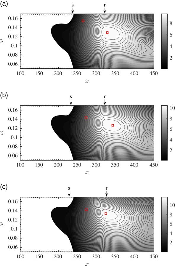
where x n is the co-ordinate for the neutral conditions (αi=0), different for each frequency ω. Figure 3 shows contours of the N-factor as a function of the streamwise co-ordinate and the frequency for three representative cases. The first of them corresponds to the two-dimensional LSB q0 with u 0,rev=6.99%, for which the primary instability is already active. The second case corresponds to the three-dimensional LSB q3D for the same reversed flow. The third case is the three-dimensional LSB corresponding to u 0,rev=7.14%. As the PSE marching is initiated in the region of zero-pressure-gradient at sub-critical conditions for T–S waves, all disturbances are initially damped. Neutral conditions are identified by the left-most boundary of the black region in the figure. The range of amplified frequencies broadens remarkably in the separated flow region, a behaviour typical of Kelvin–Helmholtz instability consistently observed in the literature(Reference Dovgal, Kozlov and Michalke5, Reference Rist and Maucher8, Reference Theofilis, Hein and Dallmann10). The figures also show the location of the maximum spatial growth rate (i.e. minimum αi, denoted by circles in the figures), that takes place upstream and at higher frequencies than the maximum amplitude (maximum N-factor, denoted by a square).
(Colour online) Convective amplification of plane T–S waves: contours of the N-factor on the (x,ω) plane. White regions correspond to stable waves. The circles correspond to the location of the maximum growth rate and the squares to the maximum amplitude. Base flows are (a) and (b) baseline LSB q0 and three-dimensional LSB q3D for u 0,rev=6.99%; and (c) three-dimensional LSB q3D for u 0,rev=7.14%. The arrows show the spanwise-averaged location of the separation and reattachement points.
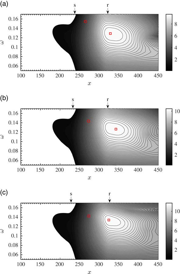
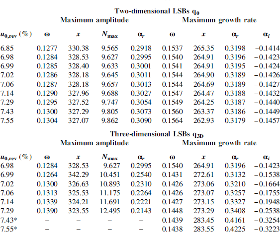
Table 1 summarises the 3D PSE computations. For each base flow considered, the conditions for the maximum amplitude and maximum growth rates are given, comprising the frequency ω, the streamwise location x and the streamwise wavenumber αr, and their respective N max and αi. PSE computations diverged towards large negative values of αi for the three-dimensional LSBs with larger reversed flows, for the range of frequencies ω≈0.14–0.15, indicating the proximity of an absolute instability. The table shows the conditions for zero group velocity, identified as saddle points in the complex α-plane(Reference Huerre and Monkewitz31). These saddle points correspond to small-amplitude negative values of ωi (not shown), denoting absolutely stable conditions but close to the critical conditions for absolute instability. As a consequence of this, the PSE integration ‘jumps’ from the downstream propagating disturbance wave to the upstream propagating one as it marches towards the saddle-point, and the results are meaningless. For u 0,rev≥7.75%, the three-dimensional LSBs become absolutely unstable giving rise to self-sustained oscillations;(Reference Rodríguez, Gennaro and Souza11) those cases are not of relevance for the present study. In the rest of the paper, only convectively unstable cases are discussed.
Conditions for the maximum amplitude and growth rate for the different two- and three-dimensional LSBs analysed using 3D PSE: frequency ω, streamwise location x and real part of the wavenumber αr, for the conditions of maximum amplitude (N max), and for maximum growth rate (−αi). The cases denoted by * correspond to conditions near absolute instability in which the PSE integration fails; the values given correspond to the saddle-point location for these cases

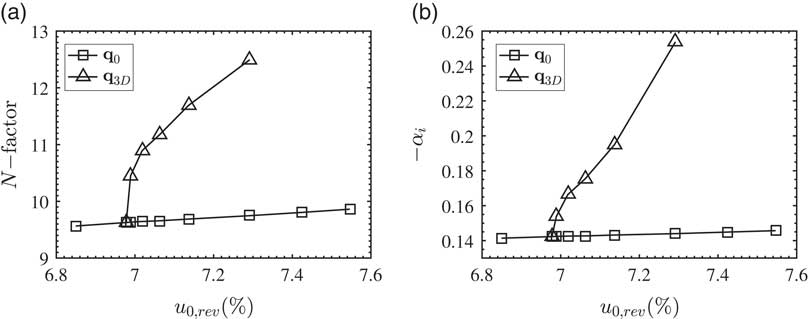
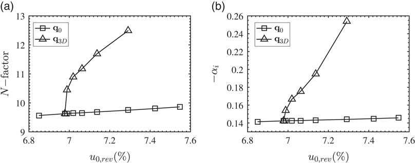
The maximum N-factor computed for each separation bubble is shown in Fig. 4(a). The maximum amplification for the two-dimensional bubbles rises moderately from N=9.57 (u 0, rev=6.85%) to N=9.86 (u 0,rev=7.55%). Conversely, a remarkable increase in the maximum amplification follows from the three-dimensionality of the separation bubble, reaching values N≈12.5 for the base flow q3D corresponding to u 0,rev=7.29%. This amounts to a 18-fold enhancement of the total disturbance amplification compared to the baseline two-dimensional bubble. Figure 4(b) shows the dependence of the maximum growth rate on the reversed flow for two- and three-dimensional base flows. Similar to the N-factors, the moderate increase in the growth rate for the two-dimensional LSBs contrasts with the strong increase in the growth rate for three-dimensional bubbles.
(a) Maximum N-factor and (b) maximum growth rate −αi for baseline LSBs q0 and three-dimensional LSBs q3D, as a function of u 0,rev.
The linear approach employed here does not provide conclusive information on the development of non-linear interactions, but they should be expected on account of the relative high N-factors, even for the two-dimensional bubbles. It is reasonable to assume that important non-linear effects will set in within the parameter range between the maximum growth rate and the maximum amplitude. Table 1 compares the streamwise location, frequency and streamwise wavenumber corresponding to the maximum growth rate and maximum amplitude, for the two-dimensional and three-dimensional LSBs. The frequency for the maximum amplitude is always lower than that of the maximum growth rate. The streamwise wavenumber is also lower; however, the difference is relatively small for two-dimensional flows. Three-dimensional LSBs present streamwise wavenumbers significantly lower for the maximum amplitude conditions, while they remain comparable to those of the two-dimensional LSBs for the maximum growth rate conditions. On the other hand, the frequencies for maximum growth rate and amplitude are significantly closer than for the two-dimensional bubbles. This seems to be a result of the reduction of the frequency for the maximum growth rate conditions on account of flow three-dimensionality.
The spatial structure of the disturbance waves corresponding to the maximum amplitude conditions is discussed next. Three-dimensional bubbles with u 0,rev=6.99–7.29% and the two-dimensional LSB with higher reversed flow, u 0,rev=7.55% ( $${\rm \bar{\rdelta }}_{{{\rm max}}} {\equals}7$$), are shown in Fig. 5. The disturbance field q′ corresponding to an individual frequency is reconstructed from the PSE computations using Equations (1) and (2). The PSE formulation used considers the velocity components, from which the spanwise disturbance vorticity field ω′z is computed and then normalised with its maximum value. The figures show instantaneous realisations of the ω′z=±0.1 surfaces. Three spanwise periods are shown in the figure, to ease the visualisation of the peak and valley structures. Note that, as a result of the large spatial amplification, disturbance waves are not visible upstream of the separation bubble with the present choice of surface level. Figure 5 also shows the u 0=0 and 0.5 streamwise velocity contours of the respective base flows.
(Colour online) Baseline LSB and eigenmode corresponding to the primary instability. Grey surfaces correspond to u 0=0 and 0.5. The surfaces correspond to instantaneous realisations of the disturbance’s spanwise vorticity field ω′z, as computed by PSE. The frequency for the maximum N-factor is considered for each case. The disturbance field is normalized so that  $$\left\Vert {{\rm \omega }'_{z} } \right\Vert_{\infty} {\equals}1$$. The surfaces shown correspond to ω′z=±0.1. Three-dimensional LSBs for u 0,rev (a) 6.99%, (b) 7.02%, (c) 7.06%, (d) 7.14%, (e) 7.29%; and (f) two-dimensional LSB for u 0,rev 7.55%.
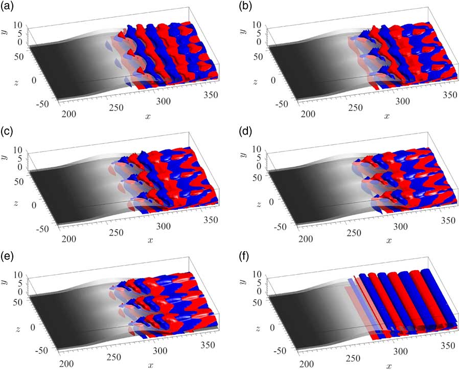
Disturbance waves, spanwise-homogeneous at introduction and upstream of separation, are distorted by the spanwise-varying separation bubble. Disturbance amplitude peaks are aligned with the spanwise planes of higher reversed flow, while the minimum disturbance amplitudes are aligned with the spanwise planes of lesser reversed flow. In the three-dimensional steady LSBs q3D, a positive streamwise streak follows downstream of the reversed-flow peak, which distorts the relative phases of the disturbance waves along the spanwise direction. The result resembles pairs of oblique waves, that seemingly arise from the peak reversed-flow locations in the figures.
Visual inspection of the 3D-PSE results indicates that the disturbance’s streamwise wavelength changes abruptly around the reattachment location for the three-dimensional LSBs. The maximum amplitudes are attained slightly downstream of reattachment, where the wavelengths are longer and typical of the attached boundary layer. These wavelengths correspond to the wavenumbers compiled in Table 1 for maximum N-factor conditions. Within the reversed flow region, wavelengths are shorter and the corresponding wavenumbers approximate the one with the maximum growth rate for each frequency. Table 2 shows the real part of the wavenumber αr inside the reversed flow region and after reattachment for the three-dimensional LSBs at their corresponding maximum amplitude frequency. The aspect ratio between the spanwise and streamwise periodicity lengths, λz/λx=αr/βc, and the obliqueness angle  $$\rphi {\equals}{\tan }^{{\minus}1} ({\rm \lambda }_{x} \,/\,{\rm \lambda }_{z} )$$ are also shown for each case. The streamwise wavelength in the reattached boundary layer increases with the baseline LSB’s reversed flow, consequently reducing the aspect ratio of the oblique waves. Conversely, in the reversed flow region downstream of the maximum wall-normal extent of the bubble, the streamwise wavenumber only a slight variation with u 0,rev, and the aspect ratio λz/λx≈1.93–2.1. These values are in excellent agreement with experimental visualisations using particle image velocimetry on LSBs formed on a flat plate(Reference Michelis, Yarusevych and Kotsonis32) and on the lee-side of an aerofoil(Reference Kurelek, Lambert and Yarusevych33), in which spanwise-modulated vortical structures were found to appear in the absence of explicit forcing.
Streamwise wavenumber, aspect ratio λz/λx=αr/βc and obliqueness angle  $$\phi {\equals}{\tan }^{{\minus}1} ({\rm \lambda }_{x} \,/\,{\rm \lambda }_{z} )$$ of the oblique disturbance waves in the reversed flow region and just after reattachment, for the frequencies of maximum total amplitude. The frequency is also given in terms of the Strouhal number Stθ.

Finally, Table 2 also shows the frequencies corresponding to maximum amplitudes in terms of the Strouhal number defined using the momentum thickness and free-stream velocity at separation, in order to allow for comparison with other results in literature. This scaling was first introduced in the context of LSBs by Pauley et al.(Reference Pauley, Moin and Reynolds34), and has been used subsequently to characterise the vortex shedding frequency. The Strouhal numbers for which the maximum amplitudes are attained lie in the range Stθ=0.0094–0.0104, which agrees well with the reported experimental measurements on unforced flat-plate LSBs(Reference Michelis, Yarusevych and Kotsonis32, Reference Henk, Reynolds and Reed35–Reference Serna and Lázaro37).
Present results show differences between the linear disturbance waves in the reversed-flow region and downstream of reattachment, where the external flow acceleration increases the phase speed, leading to a reduction in the streamwise wavelength and an increase in the obliqueness angle. Linear instability results downstream of the reattachment are of limited physical relevance, and only shown for completeness. The reason is that, following from the large convective amplifications, non-linear effects are likely to become dominant already in the reversed-flow region and give rise to intense vortical structures and turbulent transition. These vortical structures may be expected to present, initially, the characteristics of the linear waves in the reversed-flow region.
5.0 CONCLUSIONS
The convective amplification of disturbance waves by laminar separation bubbles under the influence of a three-dimensional primary deformation is addressed in this paper. Specifically, the impact of the three-dimensionalisation exerted by the self-excited primary instability of flows with recirculation on plane Tollmien–Schlichting waves is studied by means of PSE-3D computations. The necessity of using this relatively novel technique is dictated by the strong coupling between velocity components in the cross-planes, while a mild dependence of the base flow properties is allowed on the streamwise direction. Direct numerical simulations could have been applied alternatively, but their higher computational cost would have compromised the parametric study performed herein.
The primary instability sets in at reversed flows higher than u 0,rev≈6.98% and induces a spanwise-periodic modulation of the separation bubble in terms of size and recirculation intensity: while the spanwise-averaged reverse flow decreases on account of non-linearity and establishes around 6–7%, regions of increased recirculation reach peak reversed flows over 10%, which are accompanied by strong spanwise velocity gradients in the downstream half of the bubble. The three-dimensionality of the separated shear layer impacts on the amplification of disturbance waves originated upstream. The most amplified disturbances are shifted slightly to higher frequencies. In terms of the Strouhal number defined with the boundary-layer momentum thickness and free-stream velocity at separation, it changes from  $${\rm S}{\rm t}_{{{\rm \rtheta }_{{\rm s}} }} {\equals}0.0097$$ for the undisturbed baseline LSB q0 corresponding to u 0,rev=7.29%, to
 $${\rm S}{\rm t}_{{{\rm \rtheta }_{{\rm s}} }} {\equals}0.0104$$ for its corresponding three-dimensional LSB. On the other hand, the total amplification is also increased, with the maximum N-factor shifting from N=9.747 to N=12.495 for the same conditions. These results are in agreement with local instability analyses of spanwise-modulated shear layers(Reference Kawahara, Jimémez, Uhlmann and Pinelli13, Reference Saxena, Leibovich and Berkooz14).
Even more relevant than the enhancement of the linear amplification are the changes in the flow structure of the disturbance waves introduced by the three-dimensional shear-layer. The bubble’s streamwise vorticity distorts the initially two-dimensional T–S waves periodically along the spanwise direction resulting in an arrangement that resembles pairs of oblique waves with spanwise wavenumber ±βc. The location of the crests and troughs is determined by the z-co-ordinates of the recirculation minima and maxima in the steady three-dimensional LSBs, which in turn depend on the dominant spanwise wavenumber of the primary instability. The corresponding wavelength is λz/θs≈76. It should be stressed that this spanwise spacing is determined by the zero-frequency self-excited instability of the steady LSB flows(Reference Rodríguez, Gennaro and Juniper9, Reference Theofilis, Hein and Dallmann10, Reference Rodríguez and Theofilis12) and not by a secondary instability of spanwise vortices resulting from the K–H instability, as described by most experiments and simulations(Reference Diwan and Ramesh4–Reference Rist and Maucher7), or from the preferred amplification of oblique T–S waves in the pre-separated boundary layer as suggested by Michelis et al.(Reference Michelis, Yarusevych and Kotsonis32). Interestingly, similar spanwise wavenumbers have been reported in experiments considering LSBs without explicit forcing(Reference Michelis, Yarusevych and Kotsonis32, Reference Kurelek, Lambert and Yarusevych33). Finally, the combination of the dominant streamwise wavenumber, determined by the convective instability of disturbance waves, and the spanwise wavenumber associated with the self-excited centrifugal instability, define an aspect ratio of the wavy disturbances in the aft portion of the separation bubble λz/λx≈1.934–2.131, corresponding to an obliqueness angle φ≈25–27°, which again agree well with those observed in unforced experiments(Reference Watmuff16, Reference Michelis, Yarusevych and Kotsonis32, Reference Kurelek, Lambert and Yarusevych33).
The organised oblique wave pattern together with the strong spatial amplification suggests an oblique transition scenario akin to that proposed by Rist & Maucher(Reference Rist and Maucher8). They studied the non-linear interaction of a pair of oblique waves introduced upstream of an otherwise two-dimensional separation bubble, and observed that a very abrupt transition occurs. Present results show that the spanwise modulation resulting from a self-excited instability present in laminar separation bubbles has the potential of distorting initially plane T–S waves into oblique waves, promoting the same abrupt transition scenario. Here the obliqueness angle is determined by (i) the self-excited primary instability and (ii) the streamwise wavenumber corresponding to the plane T–S wave most amplified by the 3D LSB. Direct numerical simulations are currently underway to study the non-linear regimes and transition associated with this scenario.
ACKNOWLEDGEMENTS
The authors acknowledge funding from CNPq (Grants 405144/2016-4, 305512/2016-1 and 423846/2016-7), FAPESP (Grants 2014/24782-0 and 2017/01586-0) and FAPERJ (Grants 223669 and 233386).