A. BE-PFM imaging

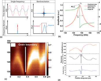
One method to overcome the difficulties with single-frequency methods is to acquire the response over the entire spectrum in parallel, the concept realized in BE family of SPMs. BE is implemented by generating a waveform consisting of multiple frequencies using a digital synthesizer. This amounts to generating a square wave with pre-defined amplitude in Fourier space, as shown in Fig. 1(a). An inverse Fourier transform is then used to generate time-domain signal that is used as an excitation to be sent to the tip. Simultaneous monitoring of the signal (over time) will give the response of the system, which can then be Fourier transformed to yield the system response over the frequency spectrum at each pixel. An example of the typical BE response at a single point is graphed in Fig. 1(b), with the raw data plotted as open circles. This can then be fit to a simple harmonic oscillator model [SHO, solid lines in Fig. 1(b)] to yield the response amplitude, phase, resonance and Q-factor at that pixel. Utilizing this method, it then becomes possible to generate BE-PFM images on time scales comparable with standard PFM.

Figure 1.

BE-PFM imaging. (a) The concept of the BE-waveform, as opposed to a single frequency measurement, in the time domain and in Fourier space. (b) Example of a single-point measurement, with raw data plotted as open circles and fitted data as solid lines. (c) A single line scan across a grain boundary, with the y-axis representing the measurement frequency. (d) Extracted profiles of amplitude, resonance frequency, and quality factor (obtained after fitting) of this line. (Images taken with the Asylum Research MFP-3D™ AFM.)

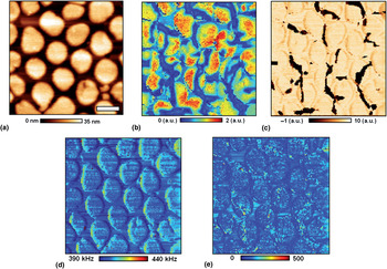
An example of BE-PFM method is illustrated in Fig. 1.^[Reference Jesse, Kumar, Kalinin, Gannepali and Proksch^80] A response along a single line scan on a sample with a grain boundary is shown in Fig. 1(c). The change in resonance across the surface is readily apparent, with a significant decrease in resonance of the order of 10 kHz in the vicinity of the grain boundary, highlighting the utility of this technique in avoiding topographical cross-talk. After SHO fitting, the amplitude, resonance frequency and quality factor profiles for this line can be extracted [Fig. 1(d)]. By collecting the response across each point in a 256 × 256 point grid, a BE-PFM image can be produced, as demonstrated in the topography, vertical BE-amplitude and phase images, as well as resonance and Q-factor of BiFeO₃ nanocapacitors in Figs. 2(a)–2(e), respectively. In this manner, the BE method decouples the cantilever transfer function related to the local mechanical properties of the material, dissipation, and total electromechanical response. The latter provides the high-veracity measure of local piezo- and ferroelectric activity.

Figure 2.

Demonstration of BE-PFM is shown in (a–c), with (a) topography, (b) BE-PFM vertical amplitude and (c) phase, along with (d) resonance, and (e) Q-factor for a collection of BFO nanocapacitors. Scale bar is 400 nm. Reprinted (adapted) with permission from Kim et al.^[Reference Kim, Kumar, Tselev, Kravchenko, Han, Vrejoiu, Lee, Hesse, Alexe, Kalinin and Jesse^81] Copyright (2011) American Chemical Society.

B. Overview of PFM spectroscopies

The characteristic aspect of BE is the rapid data acquisition rate that allows response in the frequency band to be collected at the same rate as for single frequency in classical lock-in techniques. This allows BE-PFM to be extended to a variety of different voltage and time-based spectroscopies addressing thermodynamics and kinetic aspects of polarization switching and domain wall dynamics. The necessity for complex multidimensional spectroscopic methods can be demonstrated as follows:

• • The spatially resolved measurements necessitate data acquisition over 2D dense grid of points.

• • The probing of local bias-induced transformations requires sweeping tip bias while measuring the response.

• • All first-order phase transitions (polarization switching) or wall dynamics in pinning potential are hysteretic and hence are dependent on history. This necessitates first-order reversal curve-type studies, effectively increasing dimensionality of the data (e.g., probing 2D Preisach densities).

• • First-order phase transition often possess slow time dynamics, necessitating probing kinetic hysteresis (and differentiating it from thermodynamic one) by measuring response as a function of time.

• • The detection of force-based SPMs necessitates probing response in a frequency band around resonance (since resonant frequency can be position dependent and single-frequency methods fail to capture these changes).

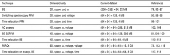
These simple physical arguments illustrate that complete PFM spectroscopies necessitate 6D [space × frequency × (stimulus × stimulus) × time] detection scheme, as compared with e.g., 1D molecular unfolding spectroscopy. To date, several 3D, 4D, and 5D detection schemes have been realized, as referenced in Table 1.

Table 1.

Development of multidimensional PFM spectroscopies.

We now proceed to discuss the 3D and higher-dimensional spectroscopies listed in the table, utilizing some examples of their applications to multiferroic materials.

C. 3D PFM spectroscopies

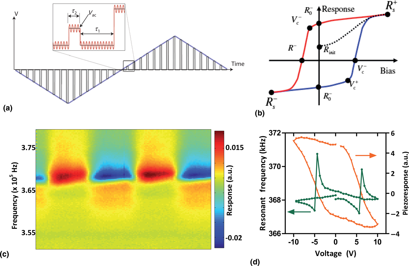
3D PFM spectroscopies are now relatively routine, and can be performed on commercially available systems. Two examples pertaining to ferroelectrics are hysteresis loop acquisition, to gauge local switching properties, and nonlinear response measurements to decipher energy loss mechanisms. The method of combining the BE method with voltage spectroscopy is shown graphically in Fig. 3(a). A step DC waveform is applied to the tip, with the BE response simultaneously applied and measured in either the on-state (τ ₂) or the off-state (τ ₁). Plotting the response as a function of the DC bias will then yield the polarization loop, from which switching parameters can be easily extracted [Fig. 3(b)].

Figure 3.

BE piezoforce spectroscopy (BEPS). (a) The general DC waveform for a measurement, with the probing AC waveform shown in inset (overlaid). The measurement can be off-field (τ ₁) or on-field (τ ₂). (b) Schematic of various fitting parameters that can be derived from a hysteresis loop. (c) A typical response from a single-point BEPS measurement. (d) Extracted piezoresponse and cantilever resonance loops from the single-point measurement in (c). Part (a) is adapted by permission from Macmillan Publishers Ltd.: Nature Materials (Jesse et al.^[Reference Jesse, Rodriguez, Choudhury, Baddorf, Vrejoiu, Hesse, Alexe, Eliseev, Morozovska, Zhang, Chen and Kalinin^91]), copyright (2008).

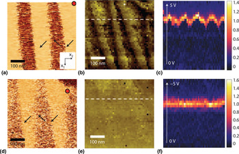
An example is shown in the spectrogram in Fig. 3(c), where the piezoresponse for a single-point measurement in a tetragonal PZT thin film is plotted. Here, the y-axis is the frequency spectrum acquired, while the x-axis corresponds to the time step (of the DC voltage sweep). The spectrogram shows that as the DC waveform is applied, the piezoresponse switches between positive (yellow, red) and negative (green, blue) multiple times, indicating polarization switching. Fitting the response to an SHO function and plotting as a function of DC voltage provides the classic ferroelectric loop, shown in Fig. 3(d). The resonance is also plotted on the same graph, for comparison. Interestingly, the resonance appears different on either side of the switching event, indicative of local strain changes as a result of ferroelastic switching. This local measurement can then be repeated across a grid of points, as shown in an example by Balke et al.^[Reference Balke, Choudhury, Jesse, Huijben, Chu, Baddorf, Chen, Ramesh and Kalinin^119] in Figs. 4(a)–4(f). In-plane (single frequency) PFM of a striped domain pattern exhibiting 71° in-plane domain walls in BiFeO₃ is shown in Figs. 4(a) and 4(d) before and after a switching spectroscopy measurement, respectively. A 50 × 50 grid of points was used with the local hysteresis loop captured at each point, and subsequently fitted to a model ferroelectric loop to yield the switching coefficients as defined in Fig. 3(b). The positive nucleation bias (V _c⁺) and negative nucleation bias (V _c⁻) were then mapped spatially in Figs. 4(b) and 4(e), respectively. It is immediately apparent that in this case, spatial variability of the nucleation bias is found only in the positive branch of the hysteresis loop. To better correlate the switching behavior with the location to the domain wall, it is useful to explore the derivative of the response with respect to voltage, along a white dashed line [Figs. 4(b) and 4(e)], i.e., we plot the line profile of ∂PR/∂V. Since the data have been collected across a voltage range, then this derivative can be plotted as a function of both voltage and spatial position, for both positive and negative branches of the loop, to yield the maps in Figs. 4(c) and 4(f). The plot confirms the influence of the domain wall in lowering the positive nucleation bias significantly. At the same time, the negative nucleation bias is entirely unaffected by the presence of the domain wall. These local insights are invaluable in determining fundamental switching mechanisms in nanoscale ferroelectrics.

Figure 4.

BEPS mapping. An example of this technique used in a mapping experiment is shown in (a–f). The in-plane PFM image (a) before and (b) after the experiment (the red dot signifies the drift of the scanner). The extracted (b) positive and (e) negative nucleation bias maps in this region. The dataset was further analyzed along the dotted white lines, with plots of ∂PR/∂V for (c) positive and (f) negative voltages along the line. Reprinted by permission from Macmillan Publishers Ltd.: Nature Nanotechnology^[Reference Balke, Choudhury, Jesse, Huijben, Chu, Baddorf, Chen, Ramesh and Kalinin^119], copyright (2009).

Voltage spectroscopy is a useful tool to study the nonlinear hysteretic behavior of ferroelectrics associated with polarization switching. However, the nonlinear response of these systems at low-to-medium driving fields (which do not cause complete polarization switching) is also of particular interest. Traditionally, these have been studied in terms of the phenomenological Rayleigh Law,^[Reference Rayleigh^25] which was shown to be near-universal for disordered ferroics.^[Reference Xu, Trolier-McKinstry, Ren, Xu, Xie and Hemker^15, Reference Damjanovic^120, Reference Damjanovic^121] The Rayleigh Law states that the susceptibility, χ, = χ_init + α _DE, where E is the applied field, and α _D is the irreversible Rayleigh constant. For ferroelectrics this law translates to a linear dependence of the piezoelectric constant on the applied field, and thus a quadratic dependence of the strain. Experiments suggested that this increase in susceptibility could be the result of motion of domain walls in the material, comprising the ‘extrinsic’ component of the piezoelectric (and dielectric) constants. The phenomenological relationship was first studied physically by Néel,^[Reference Néel^122] and then extended by Kronmüller.^[Reference Kronmüller^123, Reference Kronmüller^124] Néel assumed that the domain wall's potential energy is a statistical function of position. He determined that an interface moving through a medium with randomly distributed pinning centers would undergo reversible displacement within potential wells, as well as irreversible motion between two potential minima. The cycling between pinning and depinning of the domain wall then leads directly to a nonlinear Rayleigh response, and is the source of energy loss in the system. The theory also provides a direct physical link between the Rayleigh constant α _D and the pinning sites in the material. However, the Rayleigh model was developed for macroscopic systems, while basic questions about the nonlinear response at the microscale have remained unanswered, due to instrumental limitations.

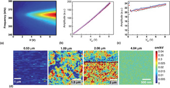
Recently, however, using the BE approach, Bintachitt et al.^[Reference Bintachitt, Jesse, Damjanovic, Han, Reaney, Trolier-McKinstry and Kalinin^102] have shown that the nonlinear response can be successfully studied with high precision at the nanoscale, which they performed on PZT thin-film capacitors of differing thickness. The technique, a 3D PFM spectroscopy, involves monitoring the BE response as a function of V _AC in the sub-switching regime, as shown in the spectrogram in Fig. 5(a). Note here that the use of BE allows monitoring of the resonance, and thus determination of material property changes (e.g., softening) as a result of the AC bias. Furthermore, it has been shown that through judicious selection of an excitation function, cantilever dynamics can be kept mostly linear,^[Reference Griggio, Jesse, Kumar, Marincel, Tinberg, Kalinin and Trolier-McKinstry^103] so that nonlinearity of the tip–surface junction can be successfully decoupled from sample piezoelectric nonlinearity. The response as a function of V _AC after fitting is shown in Fig. 5(b), with the derivative (which amounts to piezoelectric coefficient, d ₃₃ as a function of V _AC) plotted in Fig. 5(c). Remarkably, the linear dependence of the d ₃₃ on the driving field is maintained even at the nanoscale, despite the fact that the probed volume is ~10⁶ times smaller than a traditional measurement. By studying the response of PZT films of various thicknesses, it was shown that the nonlinearity appears to stem from distinct clusters of the order of 0.5–1 µm diameter in the material, which begin to appear in the 1 µm-thick sample, and grow with increasing film thickness to eventually cover the sample, as shown in Fig. 5(d). The appearance of spatial clusters of nonlinearity which grow with increasing film thickness is suggestive that Rayleigh behavior in disordered ferroelectrics is likely the result of collective dynamics, with length scales of the order of ~μm, as opposed to the motion of individual walls. The authors also found no link between d _init (the d ₃₃ at zero field) and the local nonlinearity, further suggesting that intrinsic nonlinearity cannot be the cause of Rayleigh behavior. Future studies of domain wall dynamics at the local level enabled by these BE techniques could further address 100-year-old paradigms in the field.

Figure 5.

Using BE methods to decipher collective interactions at the nanoscale. (a) 2D spectrogram of cantilever response at a single point as a function of AC bias. (b) Extracted amplitude versus bias curve. (c) The derivative is plotted, showing a linear dependence characteristic of the Rayleigh Law, for several datasets. (d) Nonlinearity maps for four PZT capacitor samples which differ in thickness (green and red colors indicate regions of high nonlinearity). It can be seen that as the thickness of the sample increases, clusters displaying nonlinear amplitude response increase in size. Adapted and reprinted with permission from Bintachitt et al.^[Reference Bintachitt, Jesse, Damjanovic, Han, Reaney, Trolier-McKinstry and Kalinin^102] Copyright National Academy of Sciences (2010).

D. 4D spectroscopy

The limitation of the standard hysteresis loop measurement is that the response is dependent on the previous state of the system, i.e., the loop is a nonanalytical function of the local control variable. Furthermore, relaxor-like responses and phenomena such as ionic diffusion tend to be associated with slow time dynamics, necessitating acquisition of datasets with multiple dimensions beyond the standard BE spectroscopic measurements. These pose instrumental challenges, in terms of fast acquisition of very large datasets, and also in methods to visualize, analyze, and interpret the data to extract the necessary parameters and their spatial variation. Here, we discuss recently developed multidimensional spectroscopies, and investigate frameworks that can be used to reduce and simplify large datasets to visualize spatial variance of the defining parameters.

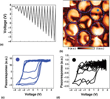
For relatively simple systems, the problem of a history-dependent response can be studied through Preisach's formalism,^[Reference Preisach^125, Reference Ge and Jouaneh^126] where hysteresis loops are modeled as a superposition of individual bi-stable switching elements (termed hysterons), with characteristic switching fields E ₁ and E ₂. The distribution of these switching fields then defines the Preisach density, which can be used to reproduce the system response to stress for any arbitrary history. Traditionally, these have been achieved on the macroscopic scale through first-order reversal curve (FORC) measurements, as shown in Fig. 6(a). Using the BE approach, we extend this concept to the microscale. In this measurement, a triangular waveform of increasing amplitude is applied and the BE response is simultaneously measured. When carried out across a grid of points, a 4D dataset is formed: the data are a function of the FORC sweep number as well as the applied bias, and the spatial coordinate (x, y). To illustrate the spatial variability in the FORC data, results from two different regions [marked by the black and blue dots in Fig. 6(b)] are shown in Figs. 6(c) and 6(d) for data captured on BFO nanocapacitors by Kim et al.^[Reference Kim, Kumar, Ovchinnikov, Jesse, Han, Pantel, Vrejoiu, Lee, Hesse, Alexe and Kalinin^127]

Figure 6.

FORC measurements using BE. (a) A triangular waveform of increasing amplitude is applied to the tip, with the BE response measured. (b) Vertical PFM amplitude of BFO nanoislands. The FORC data from the two areas marked in (b) by (c) blue and (d) black dots are shown. Reprinted (adapted) with permission from Kim et al.^[Reference Kim, Kumar, Ovchinnikov, Jesse, Han, Pantel, Vrejoiu, Lee, Hesse, Alexe and Kalinin^127] Copyright (2011) American Chemical Society.

The FORC data show that regions of downward polarization in the film show full switching [Fig. 6(c)], whereas regions of upward polarization sometimes showed incomplete switching [Fig. 6(d)]. Furthermore, it appears that all of the forward segments of the loops align, whereas the reverse segments do not, highlighting the fact that switching can proceed along many different pathways, thus necessitating a FORC-type measurement for complete characterization. By calculating the switching fields, the Preisach densities can be plotted and used to determine the system response for any history. The form of the density map can also provide an insight into the level of disorder present in the system.

E. 5D spectroscopy: dynamic PFM

The spectroscopic techniques and examples presented until now have largely ignored kinetics in the measured response. While this is appropriate in cases where thermodynamics of the switching process is the only determining factor, there exist a wide range of phenomena ranging from ionic redistribution^[Reference Kumar, Ciucci, Morozovska, Kalinin and Jesse^118, Reference Bouwmeester, Kruidhof and Burggraaf^128] in mixed ionic/electronic conductors to polarization dynamics in relaxor ferroelectrics,^[Reference Vugmeister^129] which exhibit strong time-dependent properties. Recently, Kumar et al.^[Reference Kumar, Ovchinnikov, Funakubo, Jesse and Kalinin^117] demonstrated a technique, termed as dynamic switching spectroscopy PFM (D-SSPFM) in which the thermodynamic and kinetic effects in local bias measurements can be separated.

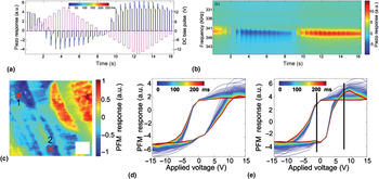
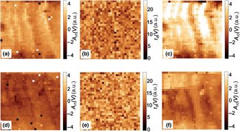
The basis of the technique is similar to the traditional BEPS measurement, in that the BE response is probed while a triangular DC waveform is applied to the material. However, in this technique, the response is measured at distinct time steps after application of each pulse, effectively adding an extra dimension to the acquired dataset. The principle is shown in Fig. 7(a), with the DC waveform shown in pink, and the response plotted after each bias pulse (as a function of t) at a single location. The corresponding spectrogram for this measurement is shown in Fig. 7(b). As can be seen, the single-point measurement takes ~17 s in total. The dataset is thus a 5D one: spatial position (x), spatial position (y), voltage, time step, and frequency bins. To illustrate the usefulness of the technique, D-SSPFM was carried out on a 2 µm-thick PZT film, shown in the out-of-plane PFM in Fig. 7(c). The response as a function of voltage and time at two locations is marked by the X in Fig. 7(c) is shown in Figs. 7(d) and 7(e), respectively. The figures indicate that there is a clear relaxation of the loop over the time scale (500 ms). However, comparing the relaxation behaviors spatially requires a reduction in the data dimensionality, which can be achieved using fitting function approaches. The relaxation data at each point can be fit to an exponential decay function, which is of the form A _r(t) = A _r0 + A _r1 exp(−t/τ_D) and thus plots of the fitting parameters can yield useful insight into spatial variances in the relaxation of the response. The plots of A _r0 (V), τ _D (V), and A _r1 (V) for the region studied are plotted in Figs. 8(f)–8(k) for V = −1 V [Figs. 8(a)–8(c)] and V = 8 V [Figs. 8(d)–8(f)]. The plots immediately reveal that the characteristic decay constant τ does not appear to have any spatial correlation, suggesting homogeneity in the relaxation mechanism. The relaxing amplitude A _r1 appears to increase with applied bias, and appears somewhat correlated with the domain structure, but not the domain walls in particular, suggesting that domain wall dynamics are not the source of the relaxation. Instead the relaxation may be related to charge injection by the tip, or bias-induced polarization rotations. These studies show the ability to separate the thermodynamic from kinetic effects, at the nanoscale, in a host of systems.

Figure 7.

Demonstration of dynamic SS-PFM. (a) The DC waveform (pink) and the response of the system (plotted in multicolor, as a function of time after the pulse). (b) The spectrogram response for a complete waveform at a single point. (c) OP-PFM image of a PZT film, with loops at (d) point 1 and (e) point 2. Reprinted with permission from Kumar et al.^[Reference Kumar, Ovchinnikov, Funakubo, Jesse and Kalinin^117] Copyright 2011, American Institute of Physics.

Figure 8.

Relaxation mapping example. Fitting maps for parameters A _r1, τ _D, and A _r0 for the region in Fig. 8 at (a–c) V = −1 V and (d–f) V = 8 V. Reprinted with permission from Kumar et al.^[Reference Kumar, Ovchinnikov, Funakubo, Jesse and Kalinin^117] Copyright 2011, American Institute of Physics.

F. Outlook

In the near future, 6D dataset acquisition will become a possibility. This will allow investigation of thermodynamics and kinetics of history-dependent systems, with nanometer precision. Additionally, more complex coupling between polarization and strain (for instance, flexoelectric effects^[Reference Kalinin, Jesse, Liu and Balandin^130, Reference Lu, Bark, Esque de los Ojos, Alcala, Eom, Catalan and Gruverman^131]) could also be studied, by e.g., measuring the responses as a function of force applied by the tip. Furthermore, we note that strong coupling between bias and strain is ubiquitous in nature and is the case for ionic solids, strongly correlated oxides, and many other systems. Correspondingly, the knowledge of dynamic processes at the nanoscale will be crucial in solving many of our current energy-related challenges. Deciphering fundamental mechanisms of reversible and irreversible transformations associated with electrochemical phenomena, such as charge ordering, bias-induced electrochemical strain, and vacancy ordering in energy materials has gained considerable attention recently with the increased research into battery technologies. Such studies are also pertinent to multiferroics, because electrochemical phenomena often appear alongside traditional polarization switching, rendering data interpretation more complex. BE techniques, and extensions such as electrochemical strain microscopy, will allow these effects to be better explored. Combining with higher dimensional spectroscopies, in which kinetic and thermodynamics information can be separated, should allow for paradigm-altering breakthroughs in energy materials.