1 Introduction
An understanding of the fate of fluid contaminants in porous geological formations is necessary in order to ensure the safe exploitation of our natural environment. The long-term transport of fluids through the subsurface is of concern in many applications of major humanitarian significance. These include the geological disposal of radioactive waste, the spoiling of freshwater reservoirs by inputs containing dissolved contaminants, the fate of fluids injected for industrial processes such as enhanced oil recovery and hydraulic fracture, and the long-term fate of supercritical
 $\text{CO}_{2}$
sequestered for geological carbon storage (Bickle Reference Bickle2009; Orr Reference Orr2009). The potential for waste products to leak and migrate from their disposal location poses major risks to maintaining environmental standards. Of particular importance is the long-term migration of
 $\text{CO}_{2}$
injected during geological carbon storage, which is key to assessing the viability of this emerging technology. To date, the analysis of fluid releases in porous media or aquifers has concentrated on cases where the medium or rock is either unsaturated or saturated with a quiescent fluid (Barenblatt Reference Barenblatt1952; Bear Reference Bear1988; Huppert & Woods Reference Huppert and Woods1995; Lyle et al.
Reference Lyle, Huppert, Hallworth, Bickle and Chadwick2005; Nordbotten, Celia & Bachu Reference Nordbotten, Celia and Bachu2005; Nordbotten & Celia Reference Nordbotten and Celia2006; Vella & Huppert Reference Vella and Huppert2006; Hesse et al.
Reference Hesse, Tchelepi, Cantwell and Orr2007; MacMinn & Juanes Reference MacMinn and Juanes2009; Golding & Huppert Reference Golding and Huppert2010; Gunn & Woods Reference Gunn and Woods2011; de Loubens & Ramakrishnan Reference de Loubens and Ramakrishnan2011a
; Pegler, Huppert & Neufeld Reference Pegler, Huppert and Neufeld2013a
, Reference Pegler, Huppert and Neufeld2014a
; Zheng et al.
Reference Zheng, Guo, Christov, Celia and Stone2015; Guo et al.
Reference Guo, Zheng, Celia and Stone2016). These studies focus on the effects of substrate topography and vertical confinement. However, they neglect a widespread feature of geological reservoirs, namely a background flow of the saturating ambient fluid. Such flows are prevalent in subsurface environments, and are driven by long-range gradients in hydrostatic pressure from surface precipitation or poroelastic deformation. We demonstrate in this paper that even slight background flow generally creates dominant long-term controls on the released fluid.
For the fundamental situation in which a two-dimensional parcel of fluid is released into a quiescent porous medium, it is found that the parcel relaxes self-similarly under gravity with its horizontal extent growing in proportion to
 $t^{1/3}$
, where
 $t$
is time (Barenblatt Reference Barenblatt1952). This solution also describes the relaxation of a parcel released on an incline in a semi-infinite porous medium (Huppert & Woods Reference Huppert and Woods1995). It is also the final regime resulting from the release of a parcel in a confined reservoir of quiescent fluid (Hesse et al.
Reference Hesse, Tchelepi, Cantwell and Orr2007). To the best of our knowledge, the general control of a background flow on the evolution of a released fluid parcel has not been considered previously. A primary result of this paper is to show that the regime determined by Barenblatt (Reference Barenblatt1952) generally fails to arise under the influence of even weak background motion, and we determine the new asymptotic regimes that arise in these new situations.
Our study begins by considering the effects of a background flow on the continuous input of fluid injected at a constant rate, as characterises the injection phase of
 $\text{CO}_{2}$
sequestration. Interesting dynamics arise in this case because the background flow and injectate compete for space within the confining porous layer. The effects of a background flow on a continuous input were considered previously by Gunn & Woods (Reference Gunn and Woods2012) for a strongly inclined aquifer, where different flow regimes can arise depending on the relative directions of the inclination and the background flow. The effect of a background flow on the rate at which a trapped region of
 $\text{CO}_{2}$
dissolves into an aquifer was considered by Unwin, Wells & Woods (Reference Unwin, Wells and Woods2016). In our analysis, we focus on the different situations of a horizontal (or broadly horizontal) substrate with a miscible contaminant, and explore the fundamental regimes controlled purely by background flow.
Capillary retention in the porous matrix can occur for a finite release of a fluid that is immiscible or partially immiscible with the ambient fluid, such as applies to a post-injection fixed-volume release of
 $\text{CO}_{2}$
into a saline aquifer (Hesse, Orr & Tchelepi Reference Hesse, Orr and Tchelepi2008; MacMinn, Szulczewski & Juanes Reference MacMinn, Szulczewski and Juanes2010). While we focus on fundamental regimes arising with negligible retention, we also conduct a short analysis developing new analytical results for the asymptotic evolution of a parcel subject to capillary retention, and the time and length scales on which a released parcel of pure
 $\text{CO}_{2}$
is retained.
A particular case of the flows we address (the special case of no background flow) concerns an as-yet-unconsidered fundamental problem of fluid injection into the interior of an aquifer bounded asymmetrically between a sealing fault and a permeable fault. Studies of injection into confined porous media to date have typically assumed a priori that the flow is axisymmetric (Nordbotten & Celia Reference Nordbotten and Celia2006; Guo et al. Reference Guo, Zheng, Celia and Stone2016) or symmetric about a linear input (equivalent to a one-sided injection) (Pegler et al. Reference Pegler, Huppert and Neufeld2014a ; Zheng et al. Reference Zheng, Guo, Christov, Celia and Stone2015). Idealisations of this kind assume symmetrical far-field conditions on the saturating fluid. However, aquifers naturally contain far-field asymmetries. For example, some faults provide a complete seal while others are permeable. An important finding of this paper is that, for a fluid-saturated aquifer, far-field asymmetries lead to dominant, almost immediate, controls on the evolution of the injected fluid. The conditions at the margins of a geological reservoir, however far away, are thus demonstrated to play a leading-order role in the evolution of fluid introduced anywhere in its interior.
We complement our theoretical results with a series of analogue laboratory experiments in which aqueous solutions of sodium chloride are injected into a confined porous bead pack saturated with fluid undergoing a pressure-driven background flow. These provide the first laboratory experiments of fluid transport with a background flow, and build on those performed previously in a quiescent medium (Pegler et al. Reference Pegler, Huppert and Neufeld2014a ). We use these experiments both to test our theoretical predictions and to develop new insights regarding additional physical effects not included in our model. These additional effects include, in particular, the role of vertical stresses and the time dependence of fluxes caused by changes in back stresses at the input points.
To demonstrate how our results can be used to inform geological problems, we apply them to some examples. As a case study, we consider the injection of natural
 $\text{CO}_{2}$
-saturated brine from a fault zone into the water-saturated Navajo Sandstone at Green River, Utah (Allis et al.
Reference Allis, White, Chidsey, Gwynn, Morgan, Adams and Moore2001; Kampman et al.
Reference Kampman, Bickle, Maskell, Chapman, Evans, Purser, Zhou, Schaller, Gattacceca and Bertier2014). The source originates from deeper reservoirs saturated by
 $\text{CO}_{2}$
, where
 $\text{CO}_{2}$
-charged brine is driven vertically through a fault by formation overpressures and leaks laterally into higher sandstone aquifers, including the Navajo. The injected brine is subsequently thought to be advected tens of kilometres or more by a background flow of water. The site provides a natural analogue for subsurface
 $\text{CO}_{2}$
transport on time scales of tens of thousands of years, thus providing a route towards understanding some long-term implications and risks of engineered geological carbon storage. We use our analytical results to assess the degree of spreading by the background flow. We also apply our results more generally to address the effect of background flow on the evolution of pure
 $\text{CO}_{2}$
injected in geological carbon storage. For typical parameter values, background flow advects
 $\text{CO}_{2}$
between one and two orders of magnitude faster than the background flow itself.
We begin in § 2 by outlining the development of our model describing the evolution of a contaminating fluid in a confined aquifer with a background flow. The equations are studied first in § 3 in the context of a continuous input of fluid, with the identification of the principal regimes arising with and without background flow. This is followed in § 4 by an analysis of the long-term migration of a fluid parcel released with fixed volume, and the various long-term modes of deformation that develop. In § 5, we present our laboratory study and comparisons with the theory. Section 6 discusses the geological implications of the results, and we conclude in § 7 by summarising the key findings.
2 Model equations
We consider a two-dimensional porous medium of uniform porosity
 $\unicode[STIX]{x1D719}$
and permeability
 $k$
saturated by an ambient fluid of density
 $\unicode[STIX]{x1D70C}_{2}$
and dynamic viscosity
 $\unicode[STIX]{x1D707}_{2}$
(figure 1). The medium is assumed to be confined by two impermeable horizontal boundaries along
 $z=0$
and
 $z=H$
. A large-scale horizontal pressure gradient drives a background flow at the volumetric flux per unit width (or depth-integrated Darcy velocity)
 $Q_{2}$
, assumed to be constant. The saturating fluid enters the medium from an input far upstream in the negative
 $x$
direction, corresponding physically to a source of fluid driven by surface precipitation, for example. The fluid is assumed to exit the medium far downstream. The special case
 $Q_{2}=0$
models the case of a sealing fault lying far upstream, which we address as a special case (§ 3). A second fluid of greater density
 $\unicode[STIX]{x1D70C}_{1}$
and viscosity
 $\unicode[STIX]{x1D707}_{1}$
is introduced through an input point at
 $x=0$
at a volumetric flux per unit width
 $Q_{1}(t)$
to form an intruding current of height
 $h(x,t)$
along the base of the medium. It should be noted that our analysis applies equally to buoyant injected fluid (e.g.
 $\text{CO}_{2}$
injected into an aquifer) on reversal of the
 $z$
coordinate. The interface between the injected and ambient fluids,
 $z=h(x,t)$
, is assumed to remain sharp.
Schematic of a dense fluid contaminant introduced into a fluid-saturated porous medium at the volumetric flux
 $Q_{1}(t)$
with a background flow of flux
 $Q_{2}$
.
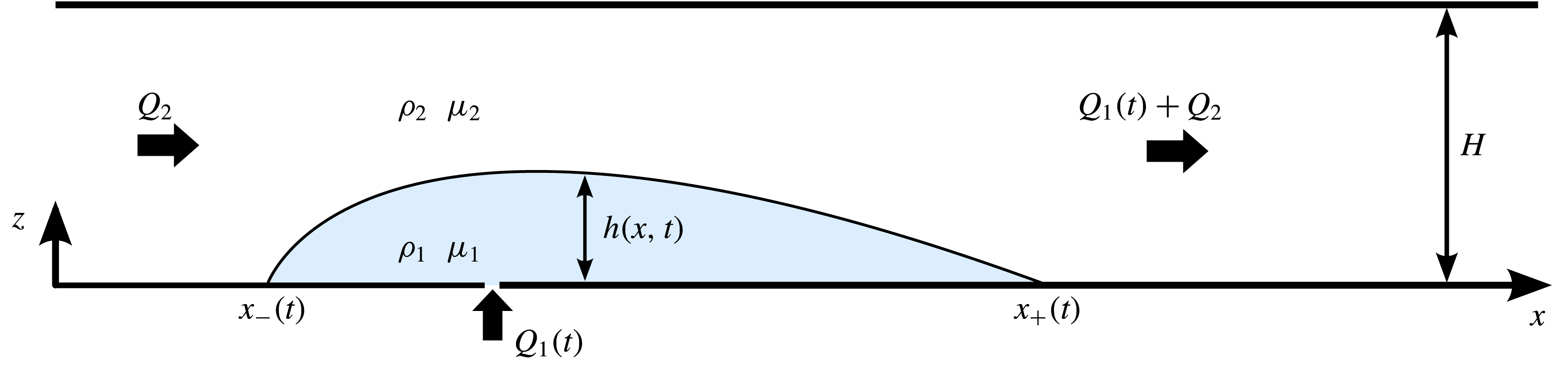
Let
 $u_{1}(x,t)$
and
 $u_{2}(x,t)$
denote the horizontal interstitial velocities of the ambient and injected fluids respectively. We model the flow using Darcy’s law and a hydrostatic-flow (Dupuit) approximation in which the horizontal velocities and pressures of the two fluid layers are given by
 $$\begin{eqnarray}u_{i}=-\frac{k}{\unicode[STIX]{x1D707}_{i}}\frac{\unicode[STIX]{x2202}p_{i}}{\unicode[STIX]{x2202}x},\quad \left\{\begin{array}{@{}ll@{}}p_{2}=P(x,t)-\unicode[STIX]{x1D70C}_{1}gz & (0\leqslant z\leqslant h),\\ p_{1}=P(x,t)-\unicode[STIX]{x1D70C}_{1}gh-\unicode[STIX]{x1D70C}_{2}g(z-h) & (h\leqslant z\leqslant H),\end{array}\right.\end{eqnarray}$$
where
 $P(x,t)$
is the as-yet-undetermined pressure along the base of the medium and
 $g$
is the gravitational strength. On substituting (2.1b
) into (2.1a
), we obtain
 $$\begin{eqnarray}u_{1}=\frac{k}{\unicode[STIX]{x1D707}_{1}}\frac{\unicode[STIX]{x2202}P}{\unicode[STIX]{x2202}x},\quad u_{2}=\frac{k}{\unicode[STIX]{x1D707}_{2}}\left(\frac{\unicode[STIX]{x2202}P}{\unicode[STIX]{x2202}x}-\unicode[STIX]{x0394}\unicode[STIX]{x1D70C}g\frac{\unicode[STIX]{x2202}h}{\unicode[STIX]{x2202}x}\right),\end{eqnarray}$$
where
 $\unicode[STIX]{x0394}\unicode[STIX]{x1D70C}\equiv \unicode[STIX]{x1D70C}_{1}-\unicode[STIX]{x1D70C}_{2}$
is the density difference between the two fluids. Mass conservation across the full depth of the medium implies that the depth-integrated horizontal velocity or volumetric flux per unit width of both fluids combined,
 $Q(x,t)$
, must be uniform throughout the regions
 $x<0$
and
 $x>0$
, with a jump of
 $Q(0_{+},t)-Q(0_{-},t)=Q(t)$
across the injection point. Upstream, the total flux is equal to the background flux
 $Q_{2}$
, and hence
 $Q(x,t)=Q_{2}$
for all
 $x<0$
. For
 $x>0$
, it equals the sum
 $Q_{2}+Q_{1}(t)$
. Hence,
 $$\begin{eqnarray}\unicode[STIX]{x1D719}[hu_{1}+(H-h)u_{2}]=Q(x,t)\equiv \left\{\begin{array}{@{}ll@{}}Q_{2} & \text{for}~x<0,\\ Q_{2}+Q_{1}(t) & \text{for}~x>0.\end{array}\right.\end{eqnarray}$$
On substituting (2.2a,b ) into (2.3) and rearranging, we determine the expression for the background pressure gradient,
 $$\begin{eqnarray}\frac{\unicode[STIX]{x2202}P}{\unicode[STIX]{x2202}x}=\left.\left[-\frac{\unicode[STIX]{x1D707}_{2}}{k}Q(x,t)+\unicode[STIX]{x0394}\unicode[STIX]{x1D70C}g(H-h)\frac{\unicode[STIX]{x2202}h}{\unicode[STIX]{x2202}x}\right]\right/[Mh+(H-h)],\end{eqnarray}$$
where
 $M\equiv \unicode[STIX]{x1D707}_{2}/\unicode[STIX]{x1D707}_{1}$
is the viscosity ratio (ambient fluid over injected fluid). By substituting (2.4) into (2.2a
), we obtain the flow rate of the injected fluid,
 $$\begin{eqnarray}u_{1}=\left.\frac{1}{\unicode[STIX]{x1D719}}\left[MQ(x,t)-U(H-h)\frac{\unicode[STIX]{x2202}h}{\unicode[STIX]{x2202}x}\right]\right/[Mh+(H-h)],\end{eqnarray}$$
where
 $U\equiv \unicode[STIX]{x0394}\unicode[STIX]{x1D70C}gk/\unicode[STIX]{x1D707}_{1}$
is the intrinsic Darcy speed at which a parcel of injected fluid falls vertically in an infinite porous medium saturated by the ambient fluid. By substituting (2.5) into the depth-integrated form of the mass-conservation equation for the lower fluid, we obtain the governing equation for the interface,
 $$\begin{eqnarray}\frac{\unicode[STIX]{x2202}h}{\unicode[STIX]{x2202}t}=-\frac{\unicode[STIX]{x2202}(hu_{1})}{\unicode[STIX]{x2202}x}=-\frac{\unicode[STIX]{x2202}}{\unicode[STIX]{x2202}x}\left[\frac{h\left(MQ(x,t)-U(H-h)\displaystyle \frac{\unicode[STIX]{x2202}h}{\unicode[STIX]{x2202}x}\right)}{\unicode[STIX]{x1D719}[Mh+(H-h)]}\right].\end{eqnarray}$$
This equation generalises those developed previously to model fluid injection or finite-volume release in quiescent porous media to allow for a spatially dependent total flux
 $Q(x,t)$
given by (2.3), which incorporates the background flow.
To specify the injection of the input fluid at
 $x=0$
, we impose
 $$\begin{eqnarray}[hu_{1}]_{-}^{+}=Q_{1}(t)\quad \text{or}\quad \left[\frac{\unicode[STIX]{x2202}h}{\unicode[STIX]{x2202}x}\right]_{-}^{+}=\frac{Q_{1}(t)}{HU}\left(M-\frac{H}{h}\right)\quad \text{at}~x=0,\end{eqnarray}$$
where the latter follows on substitution of (2.5) and simplification.
The current forms both an upstream flow front
 $x=x_{-}(t)$
and a downstream flow front
 $x=x_{+}(t)$
. To determine their evolutions, we impose the conditions of vanishing frontal thickness and kinematic rates of propagation,
 $$\begin{eqnarray}h(x_{+})=0,\quad {\dot{x}}_{+}=u_{1}(x_{+})=\frac{1}{\unicode[STIX]{x1D719}}\left(\frac{MQ(x_{+},t)}{H}-U\frac{\unicode[STIX]{x2202}h}{\unicode[STIX]{x2202}x}\right),\end{eqnarray}$$
 $$\begin{eqnarray}h(x_{-})=0,\quad {\dot{x}}_{-}=u_{1}(x_{-})=\frac{1}{\unicode[STIX]{x1D719}}\left(\frac{MQ(x_{-},t)}{H}-U\frac{\unicode[STIX]{x2202}h}{\unicode[STIX]{x2202}x}\right),\end{eqnarray}$$
where a dot denotes differentiation with respect to
 $t$
.
The injection of the current is assumed to initiate at
 $t=0$
and occur continuously at a constant rate until a total volume per unit width
 ${\mathcal{V}}$
is injected. To model this, we impose
 $$\begin{eqnarray}Q_{1}(t)=Q_{1}I(t),\quad \text{where}~I(t)=\left\{\begin{array}{@{}ll@{}}1 & (Q_{1}t\leqslant {\mathcal{V}}),\\ 0 & (Q_{1}t>{\mathcal{V}}),\end{array}\right.\end{eqnarray}$$
and
 $Q_{1}$
is a constant. Our analysis will address the cases of continuous injection (
 ${\mathcal{V}}$
infinite) and of a finite-volume input (
 ${\mathcal{V}}$
finite) separately.
2.1 Dimensionless model and representative parameter values
By forming scaling relationships between the terms in (2.6)–(2.10), we can determine the intrinsic horizontal length and time scales
 $$\begin{eqnarray}{\mathcal{L}}\equiv \frac{UH^{2}}{Q_{1}},\quad {\mathcal{T}}\equiv \frac{\unicode[STIX]{x1D719}UH^{3}}{Q_{1}^{2}}\end{eqnarray}$$
respectively, which characterise the flow of a gravity current of height
 $h\sim H$
injected into a quiescent aquifer. We use these scales to form dimensionless variables according to
 $$\begin{eqnarray}x=\left(\frac{UH^{2}}{Q_{1}}\right)\hat{x},\quad t=\left(\frac{\unicode[STIX]{x1D719}UH^{3}}{Q_{1}^{2}}\right)\hat{t},\quad h=H{\hat{h}},\quad Q=Q_{1}\hat{Q}.\end{eqnarray}$$
This choice maximises the generality of solutions to the associated dimensionless model. Recasting (2.6) in terms of (2.12) and dropping the hats, we obtain
 $$\begin{eqnarray}\frac{\unicode[STIX]{x2202}h}{\unicode[STIX]{x2202}t}=-\frac{\unicode[STIX]{x2202}}{\unicode[STIX]{x2202}x}\left[h\left(\frac{MQ(x,t)-(1-h)\displaystyle \frac{\unicode[STIX]{x2202}h}{\unicode[STIX]{x2202}x}}{Mh+(1-h)}\right)\right],\end{eqnarray}$$
where
 $$\begin{eqnarray}Q(x,t)=\left\{\begin{array}{@{}ll@{}}I(t)+B & (x>0),\\ B & (x<0),\end{array}\right.\quad \text{and}\quad I(t)=\left\{\begin{array}{@{}ll@{}}1 & (0\leqslant t\leqslant V),\\ 0 & (t>V).\end{array}\right.\end{eqnarray}$$
The input condition (2.7b ) becomes
 $$\begin{eqnarray}\left[\frac{\unicode[STIX]{x2202}h}{\unicode[STIX]{x2202}x}\right]_{-}^{+}=\left(M-\frac{1}{h}\right)I(t)\quad \text{at}~x=0.\end{eqnarray}$$
The flow-front conditions (2.8) become
 $$\begin{eqnarray}\displaystyle h(x_{+},t)=0,\quad {\dot{x}}_{+}=M[I(t)+B]-\frac{\unicode[STIX]{x2202}h}{\unicode[STIX]{x2202}x}(x_{+},t), & & \displaystyle\end{eqnarray}$$
 $$\begin{eqnarray}\displaystyle \hspace{-33.30006pt}h(x_{-},t)=0,\quad {\dot{x}}_{-}\hspace{-0.3pt}=MB-\frac{\unicode[STIX]{x2202}h}{\unicode[STIX]{x2202}x}(x_{-},t). & & \displaystyle\end{eqnarray}$$
The system depends on three dimensionless parameters,
 $$\begin{eqnarray}M\equiv \frac{\unicode[STIX]{x1D707}_{2}}{\unicode[STIX]{x1D707}_{1}},\quad B\equiv \frac{Q_{2}}{Q_{1}},\quad V\equiv \frac{{\mathcal{V}}}{Q_{1}{\mathcal{T}}},\end{eqnarray}$$
which represent the ratio of the ambient viscosity to the injectate viscosity, the ratio of the background flux to the input flux, and the dimensionless total volume of injected fluid (
 $t=V$
is the dimensionless time at which the input is stopped).
Representative parameter values for different physical situations are given as follows. The case
 $M\ll 1$
represents the case of a negligible ambient viscosity, as applies to a good approximation to hydrological problems involving the flow of water into an air-saturated aquifer, for which
 $M\approx 0.01$
. For flows involving the evolution of a solution of water charged with a contaminating solute such as sodium chloride or
 $\text{CO}_{2}$
,
 $M\approx 0.5$
–1. The converse case of a low-viscosity contaminant (
 $M>1$
) characterises the injection of supercritical
 $\text{CO}_{2}$
into a saline aquifer. As estimated in § 6,
 $M\approx 5$
–20 are typical values for
 $\text{CO}_{2}$
injection, and
 $B$
is of order unity given representative injection rates and background flow rates.
3 Continuous input
This section explores the effects of a background flow on a continuous injection of fluid (
 $V=\infty$
). In order to illustrate the essential dynamics, we solved the initial-value problem (2.13)–(2.17) numerically. A scheme was developed in which the domains upstream and downstream of the input point are each mapped onto temporally fixed domains and the derivatives in the equations are discretised using centred differences. The details of this scheme are provided in appendix A.
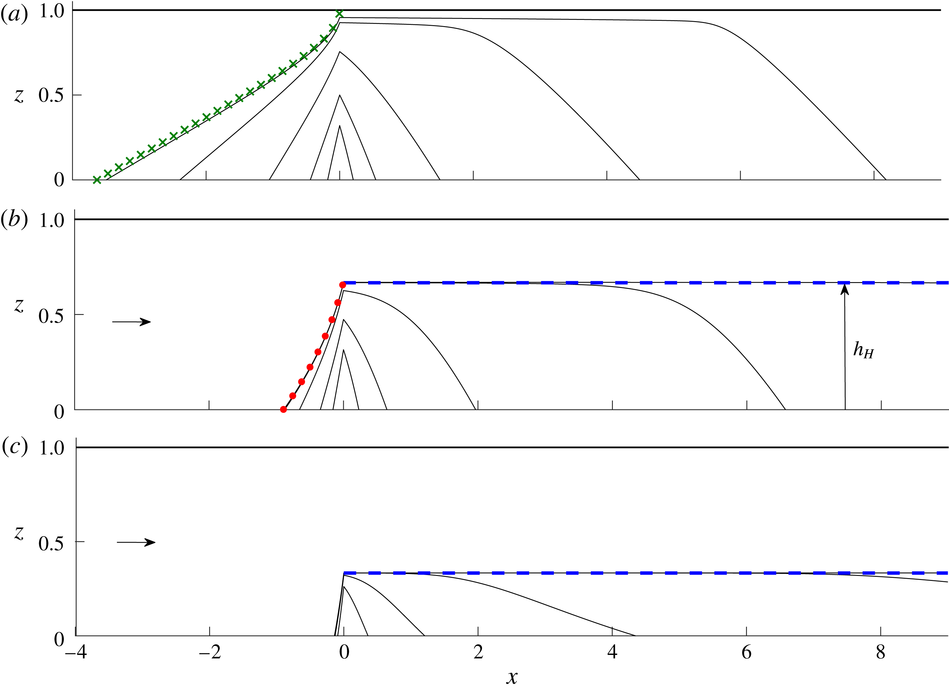
The solution for the case of no background flow,
 $B=0$
, is shown in figure 2(a). This case represents the input of fluid between a sealing fault far upstream that imposes a net volumetric flux
 $Q=0$
throughout the region
 $x<0$
in accord with (2.14a
), with the effect of producing asymmetrical far-field conditions on the saturating fluid. For illustration, we have chosen
 $M=0.5$
(injected fluid twice as viscous as the ambient fluid).
The injected current is initially symmetrical, splitting equally between leftwards and rightwards propagation. The symmetry is confirmed by the plots of
 $x_{+}(t)$
and
 $|x_{-}(t)|$
shown in figure 3(a). The initial growth conforms to an early-time similarity solution in which
 $$\begin{eqnarray}x_{+}\sim |x_{-}|\sim 1.18t^{2/3}\quad (t\rightarrow 0_{+}),\end{eqnarray}$$
which describes the continuous injection of fluid into a semi-infinite unsaturated porous medium (Huppert & Woods Reference Huppert and Woods1995). The prefactor in (3.1) has been adjusted here to account for the half–half split of the current in two directions. This similarity solution has also been determined previously to describe the early-time flow of a one-sided injection into a fluid-saturated confined porous medium in accordance with a general principle that unsaturated dynamics are recovered for
 $h\ll M^{-1}$
(Pegler et al.
Reference Pegler, Huppert and Neufeld2014a
). The general emergence of this similarity solution in the flows considered here verifies that this principle also applies in the presence of asymmetrical far-field conditions, as well as a background flow.
Numerically determined solutions to (2.6)–(2.17) describing the evolution of a fluid injected continuously for (a) no background flow,
 $B=0$
, and viscosity ratio
 $M=0.5$
(injectate twice as viscous as the ambient fluid), (b) a background flux
 $B=1$
and
 $M=0.5$
, and (c)
 $B=1$
and
 $M=2$
(injectate half as viscous as the ambient). Height profiles are shown at times
 $t=0.0625$
, 0.25, 1, 4 and 8. The long-term similarity solution describing flow towards the sealing fault for
 $B=0$
, given by our numerical solution to (3.5)–(3.6), is shown by the curve of green crosses in (a). The steady-state solution (3.11a
) is shown as a red dotted curve in (b). The prediction for the position of the horizontal interface
 $h_{H}$
given by (3.9b
) is shown as a dashed blue line in (b,c).
Distances of the positive and negative flow fronts from the injection point,
 $x_{+}(t)$
and
 $|x_{-}(t)|$
, for the solutions of figure 2. In all cases, the flow is symmetrical at early times in accord with (3.1), which is shown as a line of blue circles in each panel. The late-time asymptote (3.10) for the positive flow front
 $x_{+}$
is shown as a black dashed line in each case. In (a), the late-time asymptote for the negative flow front described by the similarity solution of § 3.1.1,
 $|x_{-}|\sim \unicode[STIX]{x1D702}_{N}t^{1/2}$
, is shown as a line of green crosses. The long-term steady position of
 $|x_{-}|$
for
 $B>0$
, as given by (3.11b
), is shown as a horizontal dotted red line in (b,c).

By
 $t=1$
, the symmetry begins to break, at which time the majority of the fluid is propagating to the right, towards the permeable fault, as
 $t$
. A slower current propagates towards the sealing fault to the left as
 $t^{1/2}$
. The break in symmetry about
 $x=0$
demonstrates a remarkable effect of the far-field conditions in providing an almost instantaneous long-range control of the direction in which the injected fluid propagates.
The solution with a non-zero background flux
 $B=1$
and
 $M=0.5$
(figure 2
b) illustrates several effects of a background flow. Early times again conform to the symmetrical self-similar growth (3.1). However, in contrast to the case
 $B=0$
, the interface does not approach the top boundary asymptotically. Instead, it forms a steady horizontal interface along the centre of the medium. The positive flow front
 $x_{+}(t)$
again grows in proportion to
 $t$
but at a faster rate than in the case
 $B=0$
. Meanwhile, the upstream flow in
 $x<0$
approaches a (stagnant) steady state of finite extent
 $-x_{-}$
, contrasting with the indefinite expansion (
 $x_{-}\rightarrow -\infty$
as
 $t\rightarrow \infty$
) occurring in the case
 $B=0$
.
The flow for
 $B=1$
and
 $M=2$
(ambient fluid twice as viscous as the injected fluid) is shown in figure 2(c). Compared with the case
 $M=0.5$
, the injected fluid forms a shallower layer. It also flows a shorter distance upstream against the background flow. Unlike the cases with
 $M=0.5$
, the current develops a broader slope, reminiscent of the profile resulting from a one-sided injection of relatively less viscous fluid into a quiescent aquifer.
3.1 Injection into a quiescent asymmetrical reservoir
We begin with a dedicated analysis of the special long-term regimes that arise with no background flow,
 $B=0$
. For this case, our solution of figure 2(a) indicated that the majority of the injected fluid eventually propagates towards the permeable fault at long times,
 $hu_{1}\sim 1$
. Therefore, the rightwards flow for
 $B=0$
approaches the same long-term regimes as a one-sided injection into a confined aquifer, as detailed by Pegler et al. (Reference Pegler, Huppert and Neufeld2014a
) and Zheng et al. (Reference Zheng, Guo, Christov, Celia and Stone2015). As determined therein, the asymptotic position of the positive flow front for
 $M\leqslant 1$
is
 $$\begin{eqnarray}x_{+}\sim t\quad (t\rightarrow \infty ),\end{eqnarray}$$
which is shown by the dashed line in figure 3(a). The general possible regimes, including those for
 $M>1$
and
 $B>0$
, will be reviewed later in the text preceding (3.10). The result of (3.2) confirms the long-term prediction of our numerical solution. In the practical context, the asymptotic regime of (3.2) will apply until the rightwards flow front interacts with the downstream end of the aquifer, beyond which time a different regime, possibly involving leakage of the current through the permeable fault, will apply. While the rightwards-propagating regime described by (3.2) is asymptotically equivalent to that of a one-sided injection towards a permeable fault, a qualitative difference is that the interface never touches the top boundary of the medium as it does in that case. A gap must persist in the present case in order to provide a conduit for fluid to escape the confined region
 $x<0$
. The gap gradually narrows over time but never vanishes completely. It should be noted that this conduit would not necessarily occur for the related problem of a point-source injection because, in that case, ambient fluid can flow around the injectate.
The solid curve shows the prefactor
 $\unicode[STIX]{x1D702}_{N}(M)$
to the frontal position
 $x_{-}\sim -\unicode[STIX]{x1D702}_{N}t^{1/2}$
describing the long-term propagation of the injected fluid in the direction of the sealed fault for the case of no background flow (
 $B=0$
) plotted against the viscosity ratio
 $M$
, obtained from numerical solutions of (3.5)–(3.6). The plot shows the decrease of the rate of propagation with
 $M$
. The horizontal dashed green line shows the asymptote
 $\unicode[STIX]{x1D702}_{N}\sim 1.62$
for
 $M\rightarrow 0$
, which represents the limit of an unsaturated aquifer. The curve of blue circles represents the asymptote for
 $M\rightarrow \infty$
given by (3.7), as predicted by the boundary-layer analysis of appendix B. The insets illustrate the self-similar profiles for
 $M=10^{-3}$
and
 $M=10^{3}$
, the latter showing the strongly concave profile that arises for large
 $M$
.

3.1.1 The self-similar flow towards the sealing fault
Figure 3(a) indicates that the leftwards current grows in proportion to
 $t^{1/2}$
, a significantly slower rate than the rightward current (3.2). To understand this evolution, it should be noted first that, as the gap above the current in the region
 $x>0$
closes, the fluid above the injection point gradually approaches the top boundary,
 $$\begin{eqnarray}h(0)\sim 1\quad (t\rightarrow \infty ).\end{eqnarray}$$
The leftwards current is therefore fed by a region of fixed height asymptotically. The long-term flow to the left can therefore be described by (2.6), (2.8a ) and (3.3). No explicit time-independent horizontal length scale can be formed from scalings of these equations, indicating a similarity solution. We define the relevant similarity variables by
 $$\begin{eqnarray}\unicode[STIX]{x1D702}=t^{-1/2}x,\quad h=h(\unicode[STIX]{x1D702}),\end{eqnarray}$$
with frontal evolution
 $x_{-}=-\unicode[STIX]{x1D702}_{N}t^{1/2}$
, where
 $\unicode[STIX]{x1D702}_{N}$
is a constant to be determined. In terms of (3.4), equation (2.13) becomes
 $$\begin{eqnarray}-\frac{1}{2}\unicode[STIX]{x1D702}h^{\prime }=\left[\frac{h(1-h)h^{\prime }}{Mh+(1-h)}\right]^{\prime },\end{eqnarray}$$
where we use a prime to denote
 $\text{d}/\text{d}\unicode[STIX]{x1D702}$
. The conditions (3.3) and (2.16a,b
) become
 $$\begin{eqnarray}h(0)=1,\quad h(-\unicode[STIX]{x1D702}_{N})=0,\quad h^{\prime }(-\unicode[STIX]{x1D702}_{N})={\textstyle \frac{1}{2}}\unicode[STIX]{x1D702}_{N}.\end{eqnarray}$$
We solved (3.5)–(3.6) numerically using a scheme in which (3.5) is integrated subject to (3.6b,c
) using the Matlab routine ode113. This integration was iterated in conjunction with a bisectional search which tunes
 $\unicode[STIX]{x1D702}_{N}$
to meet (3.6a
). The height profile and extent thus determined are shown as curves of green crosses in figures 2(a) and 3(a), and provide a close match with our numerical solution to the initial-value problem. The
 $t^{1/2}$
regime described here will cease once the current makes contact with the sealing fault, assumed to lie far in the negative
 $x$
direction; beyond that time, a no-flux condition will apply at the left-hand edge of the current, and the current will proceed to fill the left-hand section of the aquifer to long times.
The boundary-layer structure underlying the self-similar propagation of a gravity current towards a closed fault in the limit of small injectate viscosity,
 $M\rightarrow \infty$
. The case
 $M=100$
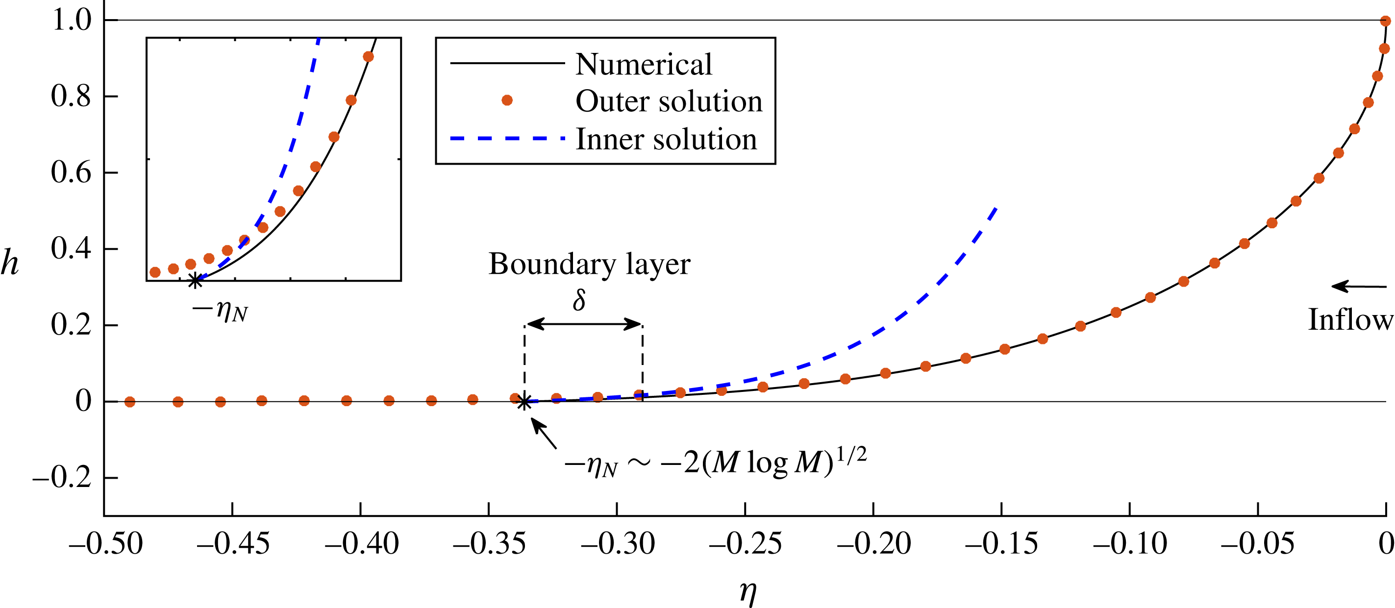
is illustrated. The numerical solution to the exact equations (3.5)–(3.6) is shown as a solid curve, with the flow front indicated by a star. As detailed in appendix B, the flow involves a boundary layer of extent
 $\unicode[STIX]{x1D6FF}\sim (M\log M)^{-1/2}$
near the flow front
 $\unicode[STIX]{x1D702}_{N}\sim 2(M^{-1}\log M)^{1/2}$
, representing a transition from a region dominated by resistance to ambient flow to a region wherein the resistance to flow of the injectate becomes leading order (and ultimately constrains the tip propagation). The outer solution satisfying (B 4a
) is shown as a dotted red curve. The inner solution (B 7), which consistently matches the outer solution to the frontal conditions (3.6b,c
), is shown as a dashed blue curve.
By solving (3.5)–(3.6) over a range of viscosity ratios
 $M$
, we determine the universal relationship between
 $\unicode[STIX]{x1D702}_{N}$
and
 $M$
shown in figure 4. For
 $M\ll 1$
, it is found that
 $\unicode[STIX]{x1D702}_{N}\sim 1.62$
. This limiting value represents the self-similar flow of a gravity current fed from a constant pressure head into an unsaturated or semi-infinite porous medium (Pritchard Reference Pritchard2007; Neufeld, Vella & Huppert Reference Neufeld, Vella and Huppert2009). It is recovered here for
 $M\rightarrow 0$
because the far-field condition of the sealing fault has no effect when
 $M=0$
. As
 $M$
increases from zero,
 $\unicode[STIX]{x1D702}_{N}$
decreases. Perhaps counterintuitively, reducing the viscosity of the current therefore decreases its rate of propagation. It should be noted that the opposite of this conclusion holds for the analogous (fixed-headed input) similarity solution describing flow towards a permeable fault (Pegler, Huppert & Neufeld Reference Pegler, Huppert and Neufeld2014b
). The coefficient
 $\unicode[STIX]{x1D702}_{N}$
instead decreases with
 $M$
here because, with a sealing fault, the current must drive a return flow of ambient fluid in order to propagate. For larger
 $M$
, the stresses associated with mobilising the return flow are larger, thus resisting the propagation of the current.
For
 $M\rightarrow \infty$
, as applies approximately to pure
 $\text{CO}_{2}$
injected into a saline aquifer, the resistance to ambient flow becomes a dominant effect. This limit produces a distinct asymptotic regime in which the evolution of the interface throughout the majority of the flow is resisted by the mobilisation of the ambient fluid. Remarkably, the viscosity of the injectate nevertheless remains important near the flow front within a small boundary layer of extent
 $\unicode[STIX]{x1D6FF}=O[(M\log M)^{-1/2}]$
, and provides the ultimate constraint on the overall rate of propagation. The mathematical analysis of this boundary-layer structure is provided in appendix B. The structure is illustrated in figure 5, where our numerical solution to the exact equations (3.5)–(3.6) for
 $M=100$
is shown alongside the inner and outer solutions determined in appendix B. The analysis reveals the asymptote
 $$\begin{eqnarray}\unicode[STIX]{x1D702}_{N}\sim 2(M^{-1}\log M)^{1/2}\quad (M\rightarrow \infty ),\end{eqnarray}$$
which is shown as a curve of circles in figure 4 and validates the numerically determined values for
 $M\gg 1$
.
3.2 The effects of background flow
The solution for
 $B=1$
and
 $M=0.5$
(figure 2
b) indicates several effects of background flow. Most evident are the development of an asymptotically steady horizontal interface in the region
 $x>0$
and the approach of the flow for
 $x<0$
towards a steady state.
To determine these asymptotic regimes, we consider the steady form of (2.6), namely
 $\unicode[STIX]{x2202}(hu_{1})/\unicode[STIX]{x2202}x=0$
. Since the long-term flow only propagates in the positive
 $x$
direction,
 $u_{1}>0$
(otherwise, the leftwards current would remain unsteady), it follows that the dimensionless flux of injected fluid
 $hu_{1}$
is equal to zero for
 $x<0$
and unity for
 $x>0$
. Using (2.5), we therefore obtain
 $$\begin{eqnarray}hu_{1}=h\left[\frac{MQ(x)-(1-h)h^{\prime }}{Mh+(1-h)}\right]=\left\{\begin{array}{@{}ll@{}}0 & (x<0),\\ 1 & (x>0),\end{array}\right.\end{eqnarray}$$
where, here,
 $h$
and
 $Q$
are functions of
 $x$
only and we have used a prime to denote
 $\text{d}/\text{d}x$
.
To seek a solution to (3.8) with a horizontal interface for
 $x>0$
, we set
 $h^{\prime }\equiv 0$
and
 $Q(x)=B+1$
, to yield
 $$\begin{eqnarray}\frac{M(B+1)h}{Mh+(1-h)}=1\quad \text{and hence}\quad h=\frac{1}{MB+1}\equiv h_{H}\end{eqnarray}$$
on making
 $h$
the subject. The height predicted by (3.9b
) is shown as a horizontal dashed line in figure 2(b,c) and matches a prevailing interior region of the numerical solution at long times. Two fluids driven simultaneously into a porous medium thus divide along a critical height
 $h_{H}$
that depends on the viscosity ratio
 $M$
and flux ratio
 $B$
between the fluids. For less viscous injectate (
 $M$
larger) or larger background flux (
 $B$
larger), (3.9b
) predicts that the height confining the lower fluid,
 $h_{H}$
, becomes smaller.
The sustained gap above the injected current effectively confines the current into a shallower quiescent aquifer of effective depth
 $h_{H}$
. Consequently, the rightwards current is asymptotically equivalent to a one-sided injection with no background flow adjusted to an effective aquifer depth
 $h_{H}=1/(MB+1)$
. To review the regimes arising for a one-sided injection with no background flow (Pegler et al.
Reference Pegler, Huppert and Neufeld2014a
; Zheng et al.
Reference Zheng, Guo, Christov, Celia and Stone2015), we recall that, in that case, the current generally grows vertically to span the depth of the medium fully. For
 $M<1$
, the two flow fronts along the top and bottom boundaries both propagate as
 $t$
at long times and form the ends of an asymptotically linear interface of constant length which is relatively short compared with the horizontal extent of the flow at long times. For
 $M=1$
, a similar regime arises except with the horizontal length of the interface growing as
 $t^{1/2}$
under the effect of gravity. For
 $M>1$
, the interface approaches a large-scale concave profile in which the front propagates at the faster rate of
 $Mt$
and the upper front at the slower rate of
 $M^{-1}t$
. With the results for the long-term frontal position adjusted to incorporate the effective aquifer height of (3.9b
), the leading position of the positive flow front with background flow can be determined as
 $$\begin{eqnarray}x_{+}\sim \left\{\begin{array}{@{}ll@{}}t/h_{H}=(1+MB)t, & \text{for}~M\leqslant 1,\\ Mt/h_{H}=M(1+MB)t, & \text{for}~M>1.\end{array}\right.\end{eqnarray}$$
The asymptotes (3.10) are shown as dashed black lines in figure 3(a–c) and agree with the large-time numerical predictions. Expression (3.10a
) shows that for
 $M\leqslant 1$
, the effect of background flow is to increase the rate of propagation of the flow front by a value
 $MB$
relative to its speed if
 $B=0$
. For
 $M>1$
, the speed of propagation is further enhanced by the extra factor of
 $M$
. For
 $M\gg 1$
, (3.10b
) has the limiting form
 $x_{+}\sim BM^{2}t$
. The value of the quadratic prefactor
 $M^{2}$
is considerable for
 $\text{CO}_{2}$
storage, with representative values lying in the range 25–400. Background flow can therefore advect injected fluid significantly faster than the background flow itself, an effect that has the potential to provide a dominant control on the migration of
 $\text{CO}_{2}$
.
To analyse the steady state arising for
 $x<0$
, we set
 $Q(x)=B$
in (3.8). By integrating that equation analytically subject to the asymptotic condition
 $h(0)\sim h_{H}$
, we obtain the steady-state height profile and negative frontal position
 $$\begin{eqnarray}h=1-[(1-h_{H})^{2}-2MBx]^{1/2},\quad x_{-}=-\frac{1-(1-h_{H})^{2}}{2MB}\end{eqnarray}$$
respectively. The predicted steady profile of (3.11a
) is shown by the curve of red circles in figure 2(b) and agrees with the numerically determined profile at long times. The corresponding agreement with (3.11b
) is shown in figure 3(b,c). Expression (3.11b
) implies that
 $|x_{-}|$
is smaller for less viscous injectate (
 $M$
larger), and hence the current propagates less far against the background flow when it is less viscous (confirmed by the comparison of the steady profiles arising for
 $x<0$
in figure 2
a,b). The regime of (3.11) is not just steady but completely static (
 $u_{1}=0$
). That is, fluid entering the upstream region
 $x<0$
never leaves it and is retained there to long times.
4 Release of a parcel
This section explores the propagation and deformation of a miscible fluid parcel following its release into a background flow (the effects of residual trapping for immiscible fluid will be considered in § 6.3). To illustrate the essential phenomena, we determined numerical solutions to the initial-value problem (2.13)–(2.17). This was done by modifying our numerical solver to perform a transition from the two-domain representation used above for
 $t<V$
to a single-domain representation
 $[x_{-},x_{+}]$
for
 $t\geqslant V$
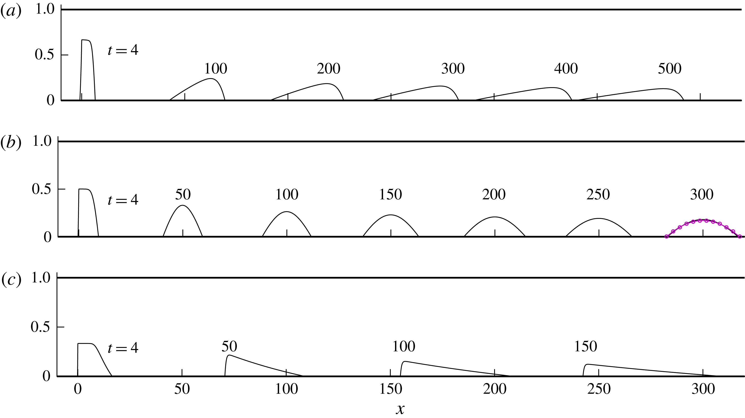
(as detailed in appendix A). Illustrative solutions for
 $V=4$
, background flux
 $B=1$
and viscosity ratios
 $M=0.5$
, 1 and 2 are shown in figure 6(a–c).
For case (a),
 $M=0.5$
, the profile resulting from the input condition rapidly smooths the interface. Relatively more fluid migrates towards the front of the parcel to produce an asymmetrical shape. The whole fluid parcel translates at approximately half the speed of the background flow. At long times, the profile steepens near the positive flow front
 $x_{+}$
. For
 $M=1$
, the parcel instead propagates at the same rate as the background flow. In this case, the current retains a fully symmetrical shape. For
 $M=2$
, the parcel is advected approximately twice as fast as the background flow. In this case, a steepened profile develops instead near the negative flow front
 $x_{-}$
.
Evolutions of fluid parcels of dimensionless volume
 $V=4$
released into a porous medium with a dimensionless background flux
 $B=1$
and viscosity ratios (a)
 $M=0.5$
, (b)
 $M=1$
and (c)
 $M=2$
, obtained from our numerical solution of (2.13)–(2.17). Times are indicated above each profile. For injected fluid more viscous than the ambient (
 $M<1$
), the parcel develops a gravity-smoothed frontal shock layer. For equal viscosities (
 $M=1$
), the profile develops a symmetrical parabolic shape in its moving frame described by the similarity solution (4.19), which is shown by the curve of purple circles at
 $t=300$
. For a less viscous injectate (
 $M>1$
), the parcel develops a trailing shock layer.
4.1 The leading-order rate of propagation of the parcel
To analyse these regimes, we begin by considering asymptotic simplifications of the model equations. It is evident from the numerical solutions that the parcel generally becomes increasingly slender with time. That is,
 $h\rightarrow 0$
and
 $\unicode[STIX]{x0394}x\rightarrow \infty$
as
 $t\rightarrow \infty$
, where
 $\unicode[STIX]{x0394}x\equiv x_{+}-x_{-}$
. Accordingly, the slope
 $\unicode[STIX]{x2202}h/\unicode[STIX]{x2202}x\sim h/\unicode[STIX]{x0394}x\rightarrow 0$
. In these limits, the gravitational contributions to the flow-front conditions (2.16b
) and (2.17b
) become asymptotically smaller than the order-unity contributions from the background flow. With regards to the leading position of the parcel, gravitational spreading can therefore be neglected. In the absence of those contributions, (2.16b
) and (2.17b
) each integrate to yield the long-term leading-order displacements of the flow fronts,
 $$\begin{eqnarray}x_{\pm }\sim MBt\quad (t\rightarrow \infty ).\end{eqnarray}$$
The parcel as a whole therefore advects at a rate of
 $M$
multiplied by the background flow rate. For geological carbon storage, the rate of advection of
 $\text{CO}_{2}$
by the background flow may be as high as
 $M=20$
times the ambient flow rate, implying an order-of-magnitude difference in velocity between the parcel and the ambient fluid. The potential for considerable differences in flow rates between the parcel and the ambient differs qualitatively from how a background flow typically affects a fluid body in non-porous fluid-mechanical configurations, for which interfacial viscous drag drives an immersed fluid parcel towards the same velocity as the background flow. The relative smallness of interfacial shear stresses in a porous medium renders that effect negligible, allowing instead for considerable velocity contrasts between the parcel and the ambient fluid.
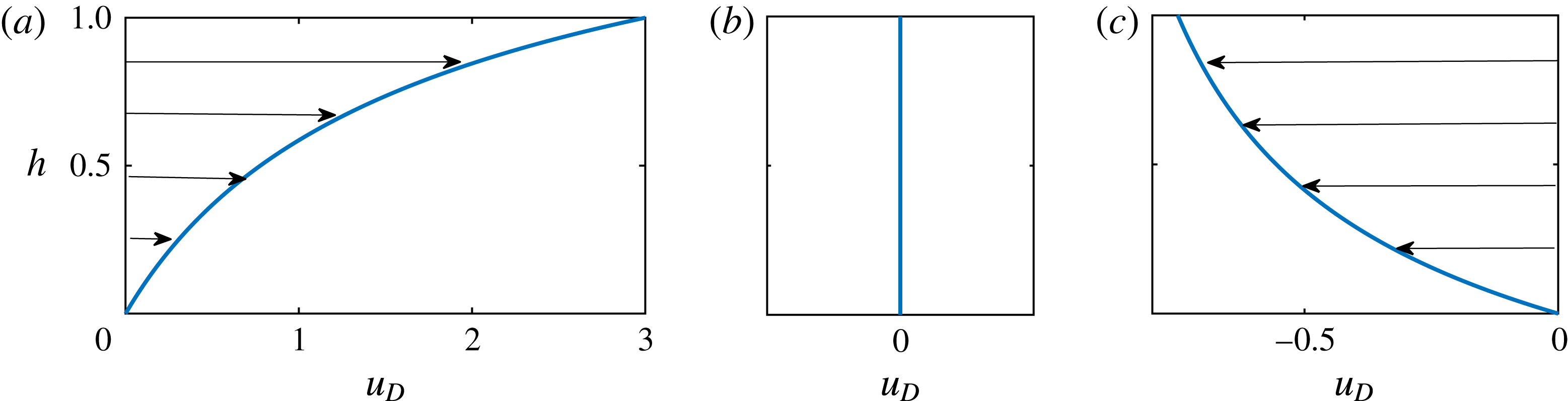
The deformation velocity
 $u_{D}(h)$
, representing the advective prefactor to the nonlinear wave equation (4.6) and the rate at which the background pressure gradient advects the interface in the frame of the parcel. The cases shown correspond to (a) a more viscous injectate,
 $M=0.5$
, (b) an equally viscous injectate,
 $M=1$
, and (c) a less viscous injectate,
 $M=2$
.
4.2 The deformation of the parcel
To explore how the parcel deforms in its moving reference frame, we recast (2.13)–(2.17) in terms of the moving coordinate system
 $(\unicode[STIX]{x1D709},t)$
, where
 $$\begin{eqnarray}\unicode[STIX]{x1D709}=x-(MB)t.\end{eqnarray}$$
In terms of these coordinates, equation (2.13) becomes
 $$\begin{eqnarray}\frac{\unicode[STIX]{x2202}h}{\unicode[STIX]{x2202}t}=MB\left(\frac{[Mh+(1-h)]^{2}-1}{[Mh+(1-h)]^{2}}\right)\frac{\unicode[STIX]{x2202}h}{\unicode[STIX]{x2202}\unicode[STIX]{x1D709}}+\frac{\unicode[STIX]{x2202}}{\unicode[STIX]{x2202}\unicode[STIX]{x1D709}}\left(\frac{h(1-h)}{Mh+(1-h)}\displaystyle \frac{\unicode[STIX]{x2202}h}{\unicode[STIX]{x2202}\unicode[STIX]{x1D709}}\right)\end{eqnarray}$$
and conditions (2.16) and (2.17) become
 $$\begin{eqnarray}h(\unicode[STIX]{x1D709}_{+})=0,\quad \dot{\unicode[STIX]{x1D709}}_{+}=-\frac{\unicode[STIX]{x2202}h}{\unicode[STIX]{x2202}\unicode[STIX]{x1D709}},\end{eqnarray}$$
 $$\begin{eqnarray}\hspace{-0.7pt}h(\unicode[STIX]{x1D709}_{-})=0,\quad \dot{\unicode[STIX]{x1D709}}_{-}=-\frac{\unicode[STIX]{x2202}h}{\unicode[STIX]{x2202}\unicode[STIX]{x1D709}}.\end{eqnarray}$$
Our numerical solutions for
 $M=0.5$
and 2 (figure 2
a,c) indicated prevailing interior regions of the parcel in which
 $|\unicode[STIX]{x2202}h/\unicode[STIX]{x2202}\unicode[STIX]{x1D709}|\ll 1$
connected to short shock layers through which
 $\unicode[STIX]{x2202}h/\unicode[STIX]{x2202}\unicode[STIX]{x1D709}$
becomes large at either the front or back of the parcel respectively. To understand this structure, we begin by considering the simplified flow regimes arising from the decay
 $\unicode[STIX]{x2202}h/\unicode[STIX]{x2202}\unicode[STIX]{x1D709}\rightarrow 0$
. Assuming that the first term in (4.3) is non-zero (
 $M\neq 1$
), this term will dominate over the second gravitational term in the limit
 $\unicode[STIX]{x2202}h/\unicode[STIX]{x2202}\unicode[STIX]{x1D709}\rightarrow 0$
, yielding
 $$\begin{eqnarray}\frac{\unicode[STIX]{x2202}h}{\unicode[STIX]{x2202}t}\sim MB\left(\frac{[Mh+(1-h)]^{2}-1}{[Mh+(1-h)]^{2}}\right)\frac{\unicode[STIX]{x2202}h}{\unicode[STIX]{x2202}\unicode[STIX]{x1D709}}\equiv -u_{D}(h)\frac{\unicode[STIX]{x2202}h}{\unicode[STIX]{x2202}\unicode[STIX]{x1D709}}.\end{eqnarray}$$
This nonlinear advection equation governs the deformation of the interface caused by the relative rates of advection of the two fluid species by the background flow. It shows that the relative rate of advection is dependent on the height of the interface separating the fluids,
 $h$
. The parcel thus evolves as a nonlinear wave with rate of advection
 $u_{D}(h)$
in the frame moving with the background flow, which we refer to as the deformation velocity. The function
 $u_{D}(h)$
is different for each value of
 $M$
, and is shown for (a)
 $M=0.5$
, (b)
 $M=1$
and (c)
 $M=2$
in figure 7. For
 $M<1$
,
 $u_{D}$
is positive, implying that fluid migrates forwards in the frame of the flow fronts. This is consistent with the development of a shock at the downstream edge. For
 $M=1$
,
 $u_{D}$
is identically zero because the background flow advects both fluids at exactly the same rate and hence does not generate the velocity contrast necessary to deform the parcel. In this special case, the advective term in (4.3) (proportional to
 $B$
) is identically zero and its assumed dominance in deriving (4.6) above is uniquely invalid; we defer addressing this case to § 4.5. For
 $M>1$
,
 $u_{D}$
is instead negative and fluid migrates backwards in the frame of the parcel, consistent with the formation of a trailing shock layer.
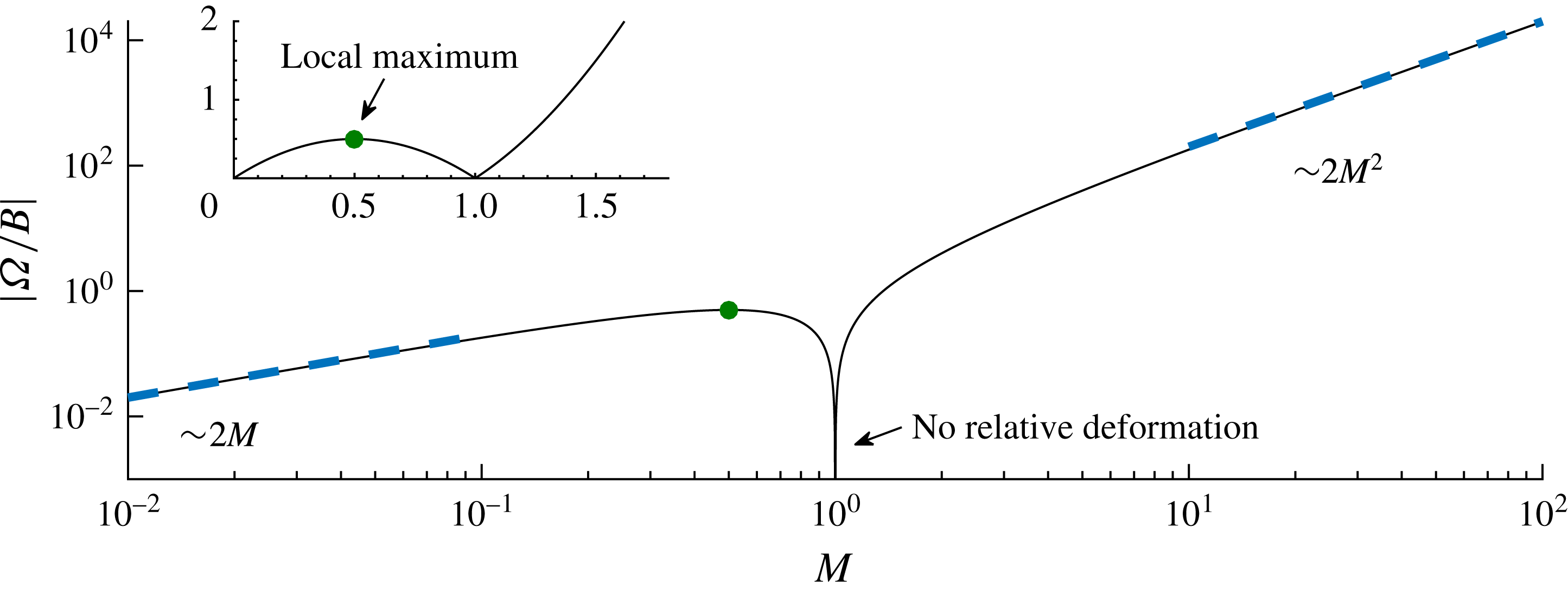
The magnitude of the stretching factor
 $|\unicode[STIX]{x1D6FA}|=2BM|1-M|$
, representing the coefficient in the nonlinear advection equation (4.7) describing the leading-order dynamics as
 $h\rightarrow 0$
and
 $M\neq 1$
. For small ambient viscosity (
 $M\rightarrow 0$
),
 $\unicode[STIX]{x1D6FA}\sim 2M\rightarrow 0$
and the background flow plays a small role in deforming the particle to leading order. For
 $M=0.5$
,
 $\unicode[STIX]{x1D6FA}$
attains a local maximum (the green circle), implying that for
 $M<1$
a fluid parcel is stretched fastest if it is exactly twice as viscous as the ambient fluid. For
 $M=1$
, the lack of viscosity contrast abruptly removes any effect of the background flow on deforming the parcel (
 $\unicode[STIX]{x1D6FA}=0$
), and the purely gravity-driven flow (in the frame of the parcel) described by the theory of § 4.5 applies uniquely. For
 $M>1$
,
 $\unicode[STIX]{x1D6FA}$
increases relatively significantly as
 $2M^{2}$
, implying the potential for considerable deformation of a parcel that is less viscous than the ambient fluid.
4.3 The self-similar horizontal stretching of the parcel
At long times, the injectate layer thins,
 $h\rightarrow 0$
, and the deformation velocity
 $u_{D}(h)$
defined in (4.6) approaches the linear asymptote
 $u_{D}(h)\sim \unicode[STIX]{x1D6FA}h$
, where
 $\unicode[STIX]{x1D6FA}\equiv 2BM(1-M)$
is the stretching parameter. In this limit, equation (4.6) reduces asymptotically to
 $$\begin{eqnarray}\frac{\unicode[STIX]{x2202}h}{\unicode[STIX]{x2202}t}\sim -\unicode[STIX]{x1D6FA}h\frac{\unicode[STIX]{x2202}h}{\unicode[STIX]{x2202}\unicode[STIX]{x1D709}},\end{eqnarray}$$
which is a simple nonlinear wave equation with prefactor proportional to
 $\unicode[STIX]{x1D6FA}$
(an inviscid Burgers equation). The absolute value
 $|\unicode[STIX]{x1D6FA}|$
measures the rate at which the background flow stretches the interface horizontally. The value of
 $|\unicode[STIX]{x1D6FA}/B|$
is plotted as a function of
 $M$
in figure 8, with the main plot showing log–log axes and the inset showing natural axes. For
 $M\ll 1$
,
 $\unicode[STIX]{x1D6FA}$
increases with
 $M$
(as
 $2M$
) because
 $M$
increases the background stress driving the deformation. However, at
 $M=0.5$
, the increase stops and
 $\unicode[STIX]{x1D6FA}$
attains a local maximum, shown as a green circle. While increasing
 $M$
still increases the ambient stress in the range
 $0.5<M<1$
, the increasing similarity between the rates at which the background flow advects the two fluid species individually as
 $M$
approaches unity causes the ambient stress to become less effective at deforming the parcel. At
 $M=1$
,
 $\unicode[STIX]{x1D6FA}=0$
because the background flow does not drive any one fluid faster than the other. The value
 $M=0.5$
is the critical value at which the increase in the background pressure gradient balances the reduction in the rate of deformation caused by the viscosities of the two fluids becoming similar. For
 $M>1$
, the viscosity contrast is reinstated and the magnitude of
 $\unicode[STIX]{x1D6FA}$
continues to increase. Ultimately, it grows as
 $2M^{2}$
, attaining values larger than those possible for
 $M<1$
.
We begin our analysis of (4.7) with the case of a relatively more viscous injected fluid,
 $M<1$
, for which
 $\unicode[STIX]{x1D6FA}>0$
. Motivated by the development of a shock layer near the front
 $x_{+}$
, we seek a solution to (4.7) subject to (2.17a
) and the volume constraint
 $$\begin{eqnarray}\int _{\unicode[STIX]{x1D709}_{-}(t)}^{\unicode[STIX]{x1D709}_{+}(t)}h(x,t)\,\text{d}x=V,\end{eqnarray}$$
with the anticipation that a conflict between the resulting solution to these equations and condition (2.16a ) produces the shock front (this will be confirmed in § 4.4 below). Since no horizontal length scale can be formed from scalings of (4.7), (2.17a ) and (4.8), one can anticipate that they support a similarity solution. To determine this, we recast these three equations in terms of the similarity variables
 $$\begin{eqnarray}\unicode[STIX]{x1D701}=\frac{x}{(\unicode[STIX]{x1D6FA}Vt)^{1/2}},\quad h=\frac{Vf(\unicode[STIX]{x1D701})}{(\unicode[STIX]{x1D6FA}Vt)^{1/2}},\end{eqnarray}$$
which yield
 $$\begin{eqnarray}\frac{1}{2}(\unicode[STIX]{x1D701}f^{\prime })^{\prime }=f\,f^{\prime },\quad f(0)=0,\quad \int _{0}^{\unicode[STIX]{x0394}\unicode[STIX]{x1D701}}f(\unicode[STIX]{x1D701})\,\text{d}\unicode[STIX]{x1D701}=1,\end{eqnarray}$$
where
 $\unicode[STIX]{x0394}\unicode[STIX]{x1D701}\equiv \unicode[STIX]{x1D701}_{+}-\unicode[STIX]{x1D701}_{-}$
. On integrating (4.10a
) subject to (4.10b,c
), we obtain
 $$\begin{eqnarray}f=\unicode[STIX]{x1D701},\quad \unicode[STIX]{x0394}\unicode[STIX]{x1D701}=\sqrt{2}.\end{eqnarray}$$
This result shows that the leading-order flow approaches a linear similarity solution with a single shock front (cf. de Loubens & Ramakrishnan Reference de Loubens and Ramakrishnan2011b
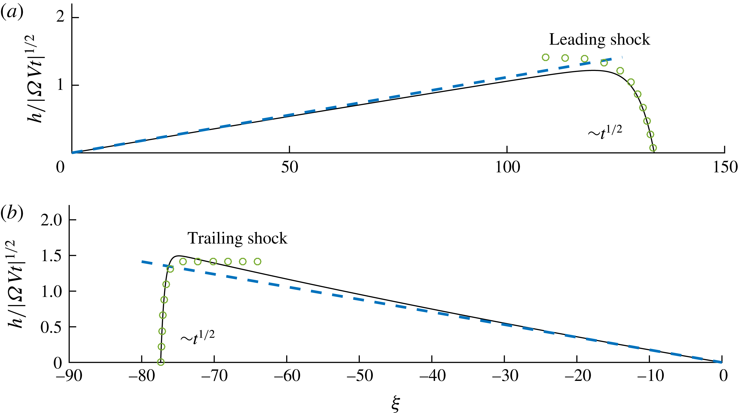
). The approach is confirmed in figure 9(a), where (4.11) is plotted as a dashed blue line and the numerical solution is shown as a solid black curve for
 $M=0.5$
at
 $t=4\times 10^{3}$
. The convergence occurs fastest near the negative flow front because the gravitational dynamics is weakest furthest from the shock layer. The evolution of the horizontal extent implied by (4.11b
) is
 $$\begin{eqnarray}\unicode[STIX]{x0394}x\sim (2\unicode[STIX]{x1D6FA}Vt)^{1/2}=2[BVM(1-M)t]^{1/2}.\end{eqnarray}$$
This result shows that the extent of the parcel grows as
 $t^{1/2}$
with a prefactor that is proportional to
 $\sqrt{\unicode[STIX]{x1D6FA}}$
and
 $\sqrt{V}$
. The parcel therefore stretches horizontally faster for larger values of the parameter
 $\unicode[STIX]{x1D6FA}$
and volumes
 $V$
.
The long-term regimes arising for (a)
 $M=0.5$
shown at time
 $t=4\times 10^{3}$
and (b)
 $M=2$
shown at
 $t=200$
, as given by our numerical solution to the full equations (2.13)–(2.16). The self-similar asymptotes describing the prevailing triangular regions, given by (4.11) for
 $M<1$
and (4.20) for
 $M>1$
, are shown by the dashed blue lines in (a) and (b) respectively. The leading-order solutions describing the gravitational smoothing of the shock fronts, given by (4.17) for
 $M<1$
, are shown by the curves of circular markers.
4.4 The shock layer
While describing the prevailing interior of the parcel, the similarity solution (4.11) conflicts with the condition of vanishing thickness at the nose (2.16a
). This conflict indicates that the second-order (gravitational) term in (4.7) remains significant near
 $x=x_{+}$
to produce a narrow ‘shock layer’ in which gravity suppresses the overturning of the interface. To investigate its intervention, we begin by considering the direct simplification of (4.3) arising from the limit
 $h\rightarrow 0$
only, namely
 $$\begin{eqnarray}\frac{\unicode[STIX]{x2202}h}{\unicode[STIX]{x2202}t}\sim -\unicode[STIX]{x1D6FA}h\frac{\unicode[STIX]{x2202}h}{\unicode[STIX]{x2202}\unicode[STIX]{x1D709}}+\frac{\unicode[STIX]{x2202}}{\unicode[STIX]{x2202}\unicode[STIX]{x1D709}}\left(h\frac{\unicode[STIX]{x2202}h}{\unicode[STIX]{x2202}\unicode[STIX]{x1D709}}\right).\end{eqnarray}$$
To study the shock layer, we transform this equation into the frame of the shock and the similarity height variable (3.4b ) by defining the horizontal coordinate and scaled height,
 $$\begin{eqnarray}X=\unicode[STIX]{x1D709}-(2\unicode[STIX]{x1D6FA}Vt)^{1/2},\quad h=(\unicode[STIX]{x1D6FA}Vt)^{-1/2}F(X).\end{eqnarray}$$
In terms of these variables, (4.13) becomes
 $$\begin{eqnarray}\frac{\unicode[STIX]{x1D6FA}}{V}\left(-\frac{F}{2t^{1/2}}+t^{1/2}F_{t}\right)-\frac{\unicode[STIX]{x1D6FA}}{\sqrt{2}}F_{X}=-\unicode[STIX]{x1D6FA}FF_{X}+(FF_{X})_{X}.\end{eqnarray}$$
To seek a solution that matches steadily to (4.11), we set
 $F_{t}=0$
. Since
 $F$
is of order unity, the first term in (4.15) decays as
 $t^{-1/2}$
and is negligible as
 $t\rightarrow \infty$
, leaving
 $$\begin{eqnarray}-\frac{1}{\sqrt{2}}\unicode[STIX]{x1D6FA}F_{X}=-\unicode[STIX]{x1D6FA}FF_{X}+(FF_{X})_{X}.\end{eqnarray}$$
By integrating this equation subject to the frontal condition (2.16a ), we obtain
 $$\begin{eqnarray}F\sim \sqrt{2}(1-\text{e}^{\unicode[STIX]{x1D6FA}(x-x_{+})/2}).\end{eqnarray}$$
This solution is shown as a curve of green circles in figure 9(a) and successfully describes the profile through the shock layer. Expression (4.17) shows that the extent of the shock is of
 $O(\unicode[STIX]{x1D6FA}^{-1})$
, implying, in particular, that a stronger background flow creates a shorter shock layer. This length scale remains constant in time but, since
 $\unicode[STIX]{x0394}x$
given by (4.12) increases with time, the shock layer becomes increasingly smaller relative to the horizontal extent of the parcel as a whole as
 $t\rightarrow \infty$
. Equation (4.17) predicts that
 $F\rightarrow \sqrt{2}$
as
 $x\rightarrow -\infty$
. This confirms a correct matching between (4.17) and the value of the outer solution (4.11) in the limit
 $\unicode[STIX]{x1D701}\rightarrow \sqrt{2}$
, in accordance with van Dyke’s matching rule.
4.5 Equally viscous input and ambient fluids
As noted above, for
 $M=1$
, the background flow advects the injected fluid at exactly the same rate as the background flow itself. Its effect in deforming the parcel, represented by the first term on the right-hand side of (4.3), is therefore identically zero. In this unique case, the assumption that the gravitational term in (4.3) becomes negligible as the slope of the parcel decreases is invalid. Instead, (4.3) simplifies to
 $$\begin{eqnarray}\frac{\unicode[STIX]{x2202}h}{\unicode[STIX]{x2202}t}=\frac{\unicode[STIX]{x2202}}{\unicode[STIX]{x2202}\unicode[STIX]{x1D709}}\left(h(1-h)\displaystyle \frac{\unicode[STIX]{x2202}h}{\unicode[STIX]{x2202}\unicode[STIX]{x1D709}}\right)\sim \frac{\unicode[STIX]{x2202}}{\unicode[STIX]{x2202}\unicode[STIX]{x1D709}}\left(h\frac{\unicode[STIX]{x2202}h}{\unicode[STIX]{x2202}\unicode[STIX]{x1D709}}\right)\quad (h\rightarrow 0),\end{eqnarray}$$
and describes a purely gravity-driven relaxation of the parcel in the frame of the background flow. In its moving frame, the parcel therefore relaxes exactly as if in a quiescent porous medium. As determined by Barenblatt (Reference Barenblatt1952), this equation, along with the volume constraint (4.8), supports the exact similarity solution
 $$\begin{eqnarray}h=\left(\frac{3}{32}\frac{V^{2}}{t}\right)^{1/3}\left[1-\left(\frac{2}{9Vt}\right)^{2/3}\unicode[STIX]{x1D709}^{2}\right],\quad \unicode[STIX]{x0394}x=(36Vt)^{1/3}.\end{eqnarray}$$
This dome-shaped profile is shown as a curve of purple circular markers in figure 6(b). It confirms the leading-order symmetrical relaxation of the parcel in a frame moving with the background flow. It should be noted that the rate of relaxation
 $\unicode[STIX]{x0394}x\propto t^{1/3}$
predicted by (4.19b
) is slower than the rate
 $\unicode[STIX]{x0394}x\propto t^{1/2}$
predicted by (4.12) for
 $M\neq 1$
. The effect of the background flow in directly stretching a released parcel for
 $M\neq 1$
thus drives a greater rate of horizontal extension than would occur by gravity acting independently.
4.6 Less viscous input fluid
For
 $M>1$
, the first term in (4.3) is non-zero, and hence, like the cases of
 $M<1$
, it becomes dominant at late times. Likewise, the resulting simplified equation (4.7) describes the leading-order dynamics. The only difference is that the stretching factor
 $\unicode[STIX]{x1D6FA}$
is negative if
 $M<1$
. That is, the background flow advects higher fluid backwards in the frame of the parcel. To address this case, we repeat the steps of the analysis of § 4.3 above, except with
 $\unicode[STIX]{x1D6FA}$
replaced by its absolute value
 $|\unicode[STIX]{x1D6FA}|$
in (4.9), and applying (2.16a
) instead of (2.17a
). The analysis determines the similarity solution
 $$\begin{eqnarray}f=-\unicode[STIX]{x1D701},\quad \unicode[STIX]{x0394}\unicode[STIX]{x1D701}=\sqrt{2}.\end{eqnarray}$$
Like (4.11), (4.20) describes a triangular profile. However, its gradient is opposite to the case
 $M<1$
and thus predicts a shock at the negative flow front instead of the positive flow front. The asymptotic approach of our numerical solution towards (4.20) is confirmed in figure 9(b), where (4.20a
) is shown as a dashed blue line at
 $t=200$
. The time of transition towards the similarity solution is faster for
 $M=2$
than
 $M=0.5$
because the magnitude of the stretching parameter
 $|\unicode[STIX]{x1D6FA}|=2$
is four times larger. For
 $M>1$
, there is no maximum value of
 $|\unicode[STIX]{x1D6FA}|$
, contrasting with the case
 $M<1$
, for which it was noted that there is a maximum at
 $M=0.5$
. Background flow thus has the potential to provide significantly greater rates of stretching when the parcel is less viscous than the ambient fluid compared with cases where it is more viscous.
5 Experimental study
A series of laboratory experiments was conducted to confirm aspects of the model predictions and to assess the significance of further mechanical considerations not incorporated within our model. The experiments were conducted in an acrylic tank with dimensions of length 200 cm, height 25 cm and internal spacing 0.6 cm (figure 10). Spacers confined a region of internal height 10 cm that was fully enclosed except for a 10 cm horizontal gap at the right-hand edge of the upper confining boundary. This enclosed region was filled with glass beads of diameter 2 mm to create a porous medium. The mean porosity was
 $\unicode[STIX]{x1D719}\approx 0.38\pm 0.01$
and the mean permeability was
 $k\approx 3.1~(\pm 0.2)\times 10^{-5}~\text{cm}^{2}$
(Pegler et al.
Reference Pegler, Huppert and Neufeld2014a
).
Schematic of our experimental system.
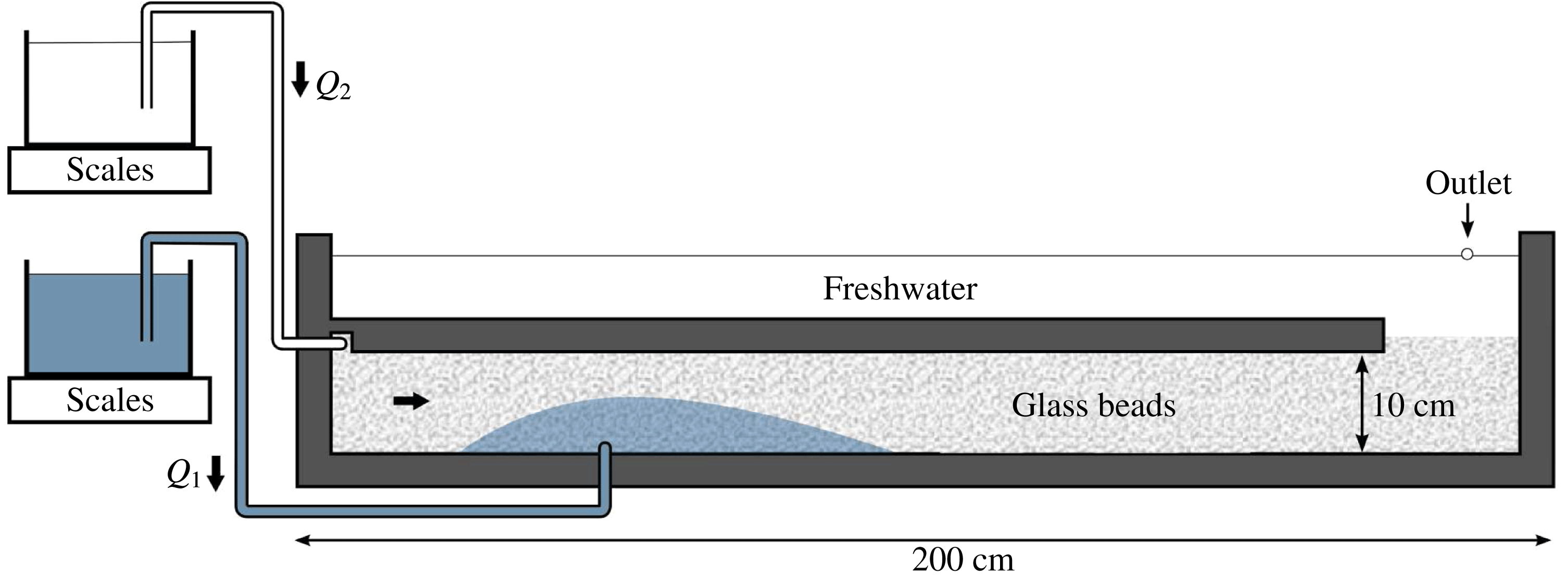
For the saturating ambient fluid, we used freshwater of density
 $\unicode[STIX]{x1D70C}_{2}=0.998$
(
 $\pm 0.001$
)
 $\text{g}~\text{cm}^{-3}$
and viscosity
 $\unicode[STIX]{x1D707}_{2}\approx 0.93{-}0.99~(\pm 0.01)~\text{g}~\text{cm}^{-1}~\text{s}^{-1}$
, which were measured before each set of experimental runs using a hydrometer and a U-tube viscometer respectively. For the injected fluid, we used denser (and more viscous) solutions of water and sodium chloride to create density differences of
 $\unicode[STIX]{x0394}\unicode[STIX]{x1D70C}=0.069{-}0.178~(\pm 0.001)~\text{g}~\text{cm}^{-3}$
and injectate viscosities of
 $\unicode[STIX]{x1D707}_{1}\approx 1.16{-}1.72$
(
 $\pm 0.01$
)
 $\text{g}~\text{cm}^{-1}~\text{s}^{-1}$
.
A continuous input of ambient fluid was achieved using a raised reservoir of freshwater connected via a syphon to the inlet at the upper left-hand corner of the enclosed region. The hydrostatic head in the reservoir was maintained to create a fixed input pressure, and the mass of the reservoir was continuously monitored to determine the input flux per unit width
 $Q_{2}(t)$
. The ambient fluid partially filled an open region above the porous medium. An outlet in the face of the cell allowed fluid to overspill through a large exit tube and thus fixed the hydrostatic head of the upper surface of the ambient fluid over time. With the background flow already initiated, the dyed salty water was injected through an inlet at the base of the medium at a distance of 40 cm from the left-hand edge. The injection flux
 $Q_{1}(t)$
was determined analogously to the background flux. Two sets of experiments were conducted. In the first set (runs 1–6), the injection was continued until the end of the experiment (
 ${\mathcal{V}}=\infty$
). Across these runs, the hydrostatic head of the fluids in the reservoirs was varied to create a variety of input rates. In the second set (runs 7–8), we terminated the injection once a finite volume per unit width
 ${\mathcal{V}}$
was input. Each experiment was recorded using a digital camera with time-lapse photography.
(a) The volume per unit width of fluid injected into the tank, as inferred from the mass reading for the reservoir of dyed injected fluid over the course of experiment 4. The dotted curve shows the raw data. The solid blue curve shows the fitted least-squares parabola. (b) The associated linear change in
 $Q_{1}(t)$
implied by the derivative of the fitted parabola, which we used to determine the constants
 $Q_{1}^{(0)}$
and
 $\unicode[STIX]{x1D6FC}_{1}$
in (5.1a
).
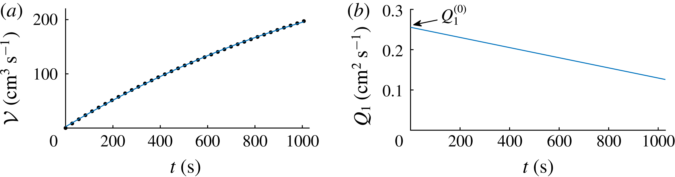
Analysis of the mass readings of the feeding reservoirs showed some temporal changes in the rates of input of both the ambient and injected fluids over the course of each experiment. Since the pressure heads at both input points were effectively constant, we anticipate that the reduction of the input rates is a physical effect of the tank becoming filled with the relatively more viscous fluid, which increases the resistance to driving both fluids into the tank. An illustrative example of a decrease in the rate of dyed fluid is shown for experiment 4 in figure 11. A least-squares parabola provides a good fit to the data, as shown overlaid as a solid curve in figure 11(a), with similar fits applicable to all of runs 1–6. The corresponding linear relationships for the input and ambient fluxes (illustrated for
 $Q_{1}(t)$
in figure 11
b) are
 $$\begin{eqnarray}Q_{1}(t)\approx Q_{1}^{(0)}-\unicode[STIX]{x1D6FC}_{1}t,\quad Q_{2}(t)\approx Q_{2}^{(0)}-\unicode[STIX]{x1D6FC}_{2}t,\end{eqnarray}$$
where
 $Q_{1}^{(0)}\equiv Q_{1}(0)$
and
 $Q_{2}^{(0)}\equiv Q_{2}(0)$
are the fluxes at
 $t=0$
, and
 $\unicode[STIX]{x1D6FC}_{1}$
and
 $\unicode[STIX]{x1D6FC}_{2}$
are constants determined from the least-squares fit. In order to incorporate this variation within our model, we apply (5.1) in place of (2.3). With the same non-dimensionalisation (2.12), except with the initial flux
 $Q_{1}^{(0)}$
in place of
 $Q_{1}$
, the augmented dimensionless model is given by generalising (2.14) to
 $$\begin{eqnarray}\hat{Q}(\hat{x},\hat{t})=\left\{\begin{array}{@{}ll@{}}B(\hat{t})+I(\hat{t}) & (\hat{x}<0),\\ B(\hat{t}) & (\hat{x}>0),\end{array}\right.\quad \text{where}\,\left\{\begin{array}{@{}l@{}}I(\hat{t})=1-A_{1}\hat{t},\\ B(\hat{t})=B_{0}-A_{2}\hat{t}.\end{array}\right.\end{eqnarray}$$
These specifications depend on the initial ratio of background fluxes,
 $B_{0}\equiv Q_{2}^{(0)}/Q_{1}^{(0)}$
, and two dimensionless rates of change,
 $A_{i}\equiv \unicode[STIX]{x1D6FC}_{i}{\mathcal{T}}/Q_{1}^{(0)}$
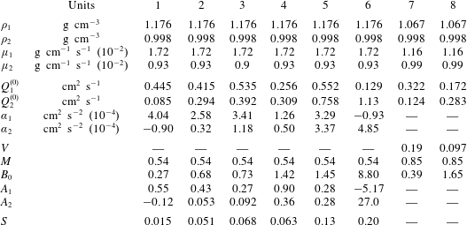
, which are listed for each experiment in table 1. No significant variation in flux was evident in the finite-volume release experiments 7 and 8. This is expected because the volume of the more viscous dyed fluid inputted was sufficiently small in these experiments that any increase in the resistance to driving fluid into the tank was negligible.
Parameter values used in our laboratory experiments. The first set of experiments (runs 1–6) involved a sustained continuous input (
 $V=\infty$
). The second set (runs 7 and 8) involved a finite-volume release (
 $V$
finite). The two sets are individually listed from left to right in ascending order of initial dimensionless background flux
 $B_{0}$
.
5.1 Experimental results and theoretical comparisons
The evolution of a representative experiment (run 4) is shown as a time-lapse sequence in figure 12. The experiment is also shown in the supplementary movie available at https://doi.org/10.1017/jfm.2017.501. In agreement with the theory, the current is initially close to symmetrical and subsequently develops a shorter component flowing upstream against the background flow and a larger component flowing downstream with the background flow. An approximately sharp interface between the injected and ambient fluids is retained. Some slight fading at the downstream flow front indicates a stronger effect of hydrodynamic dispersion in smearing the interface for regions where the current displaces the ambient fluid. The theoretical height profiles given by our numerical solution to the model (2.13)–(2.17) and (5.2) are overlaid as white dashed curves; generally good agreement is observed.
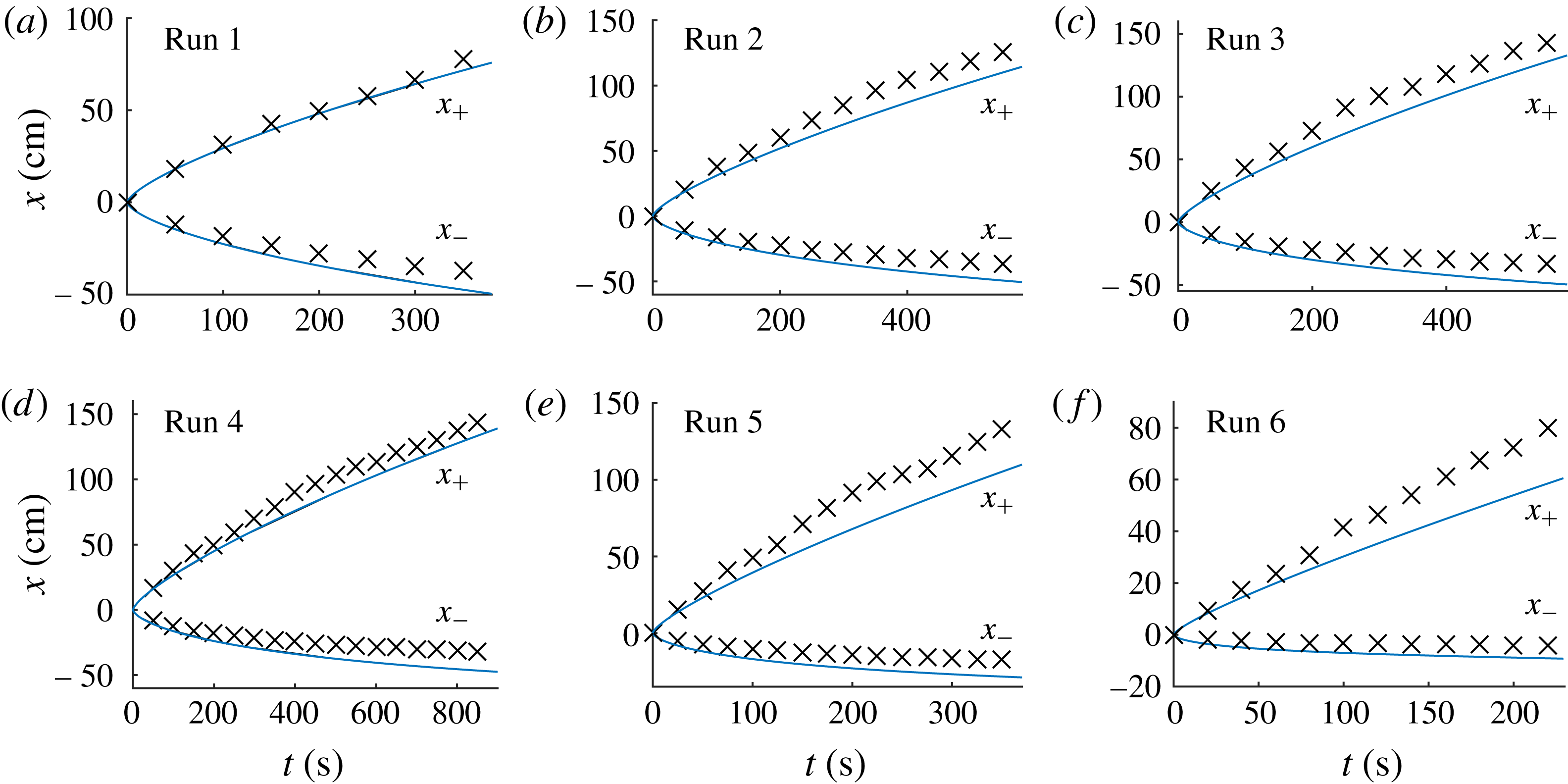
Some discrepancies between the theory and the data occur mainly along the upstream interface, where the theory overpredicts the distance propagated by the negative flow front
 $|x_{-}|$
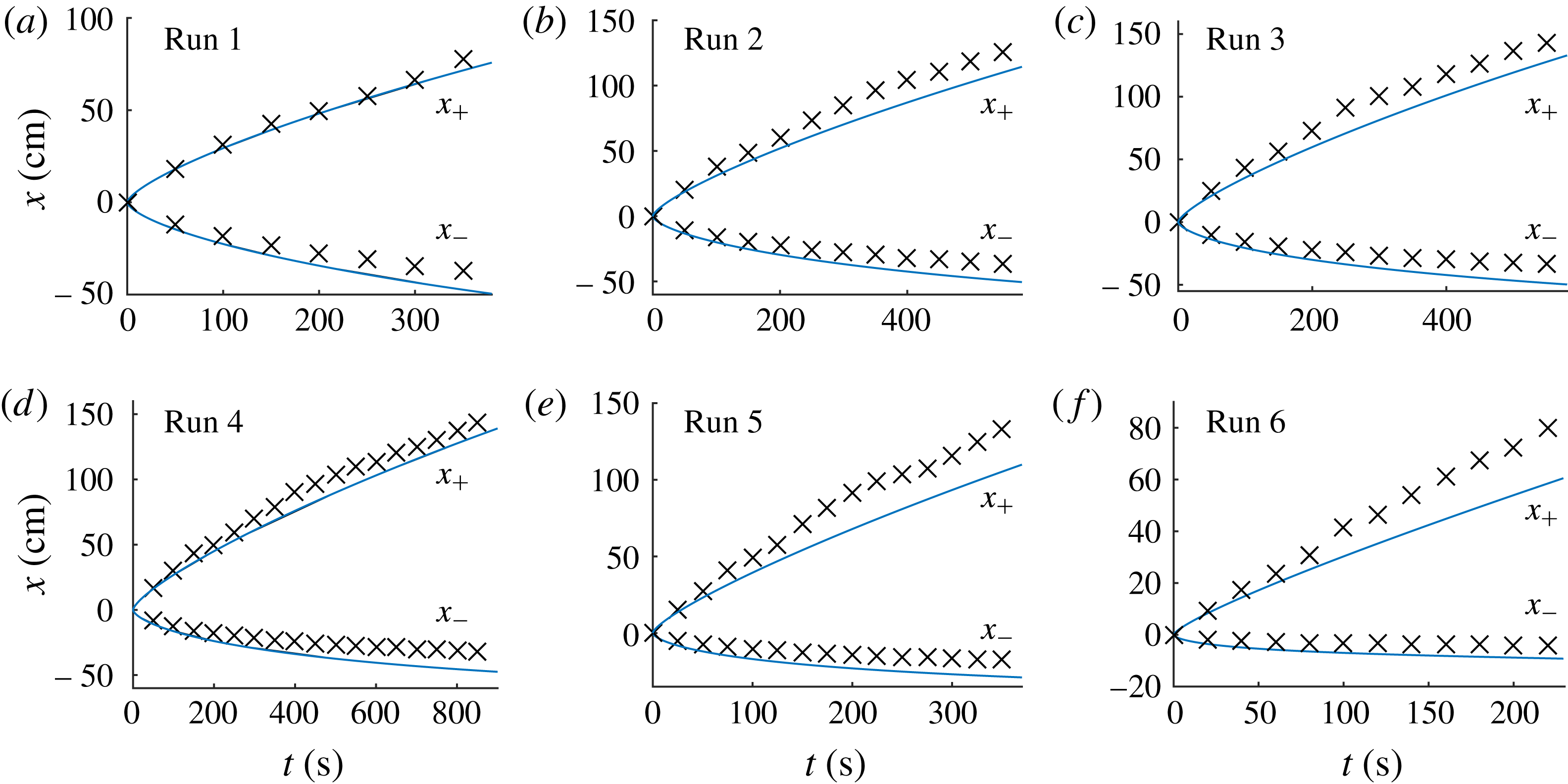
. This trend is illustrated for all of our continuous-input experiments in figure 13, where the positions of the positive and negative flow fronts measured from the digital images and predicted by our theory are shown together. The experiments with larger background flow tend to produce larger discrepancies. We conjecture that the discrepancy is caused by stresses associated with vertical flow weakening the (Dupuit) approximation of hydrostatic pressure; this hypothesis is considered in detail below. Since less fluid propagates upstream than predicted by the theory, correspondingly more fluid flows downstream. This explains the slight underprediction of the position of the downstream flow front observed for each experiment.
Time-lapse sequence of photographs showing a representative experiment (run 4) at times (a) 80 s, (b) 200 s and (c) 800 s after the injection of the dyed salty water was initiated. The dyed fluid, introduced at
 $x=0$
, is advected through the bead pack by an ambient background flow of the saturating clear freshwater. The vertical aspect has been stretched by a factor of two. The theoretical prediction of the full numerical model given by (2.13)–(2.17) with (5.2) in place of (2.14) is overlaid as a white curve in each panel.


Time-lapse sequence showing a representative finite-volume release (run 7) at (a) the time
 $t=140$
s at which the input is terminated and (b)
 $t=1800$
s. The vertical aspect has been stretched by a factor of two. The theoretical prediction of the full numerical model given by (2.13)–(2.17) with (5.2) in place of (2.14) is overlaid as a white curve in each panel.

Comparisons between the experimental data (crosses) and theoretical predictions (solid curves) of the model (2.13)–(2.17) for the negative and positive flow fronts,
 $x_{-}$
and
 $x_{+}$
, measured for experimental runs 7 and 8. In these runs, the inputs were terminated at the times indicated by the vertical dashed lines to create a finite-volume release.
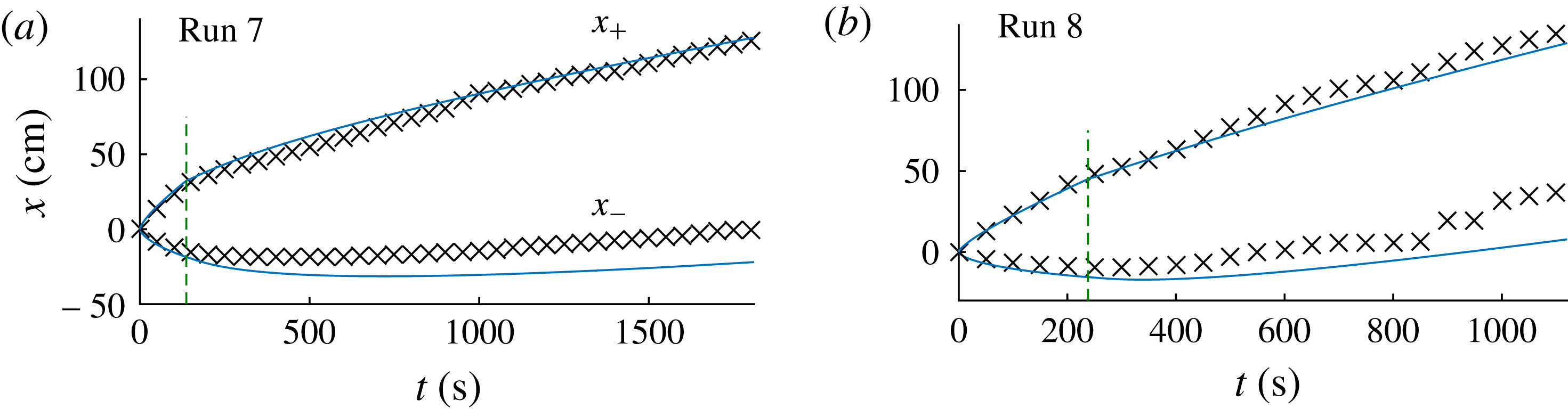
A time-lapse sequence of the finite-volume experiment (run 7) is shown in figure 14. The flow-front evolutions for both finite-volume experiments (runs 7 and 8) are shown in figure 15, where the times at which the input ceases are shown as vertical dashed lines. The plots show good agreement with the theoretical predictions. Again, some discrepancies occur near the negative flow front, which persist as the parcel advects downstream. For run 8, the negative flow front
 $x_{-}$
propagates relatively further downstream and is observed to leave small patches of the injected fluid behind its trailing edge. The patches remain for a short period of time before being swept away by the ambient fluid. The phenomenon is indicated by the step-like progression of
 $x_{-}$
that occurs for
 $t>600$
s in figure 15(b), which measures the distance furthest upstream at which a patch is observed and lags intermittently behind the bulk of the parcel. We anticipate that these patches arise as a consequence of localised regions of lower permeability in the bead pack, which intermittently trap patches of the parcel as it passes through.
5.2 The role of vertical stresses
Analysis of the runs involving a continuous input revealed a persistent, if relatively small, discrepancy between the data and the theory in the position of the negative flow fronts. We anticipate that this discrepancy is a consequence of a weakening of the assumption of predominantly horizontal flow (the Dupuit approximation) caused by a large interfacial slope at the negative flow front. In the extreme limit of a large background flow, the interaction between the ambient flow and the injected fluid would more closely approximate the flow around a locally vertical boundary created by the injected fluid, with the ambient fluid just upstream of the negative flow front
 $x_{-}$
being directed vertically in a stagnation-point flow. Stresses associated with this vertical flow weaken the assumption of hydrostatic pressure (2.1b
) underlying the theory.
In steady state, the flow along the upstream interface is tangential to the interface. Therefore, we can anticipate that the significance of the vertical flow is measured by the magnitude of the gradient of the interface
 $\unicode[STIX]{x2202}h/\unicode[STIX]{x2202}x$
at the negative flow front
 $x_{-}$
. Using (3.11b
), the model prediction for the magnitude of this gradient is
 $$\begin{eqnarray}\frac{\unicode[STIX]{x2202}h}{\unicode[STIX]{x2202}x}=MB\frac{H}{{\mathcal{L}}}=\frac{\unicode[STIX]{x1D707}_{2}Q_{2}}{\unicode[STIX]{x0394}\unicode[STIX]{x1D70C}gkH}\equiv S,\end{eqnarray}$$
where
 $S$
is a dimensionless number that we refer to as the background flow strength. The self-consistency of the model depends on
 $S\ll 1$
, with larger values of
 $S$
predicting a larger deviation from hydrostatic pressure. A similar dimensionless parameter to (5.3) was used by Pegler et al. (Reference Pegler, Kowal, Hasenclever and Worster2013b
) to explain discrepancies due to vertical stresses for the related problem of a transition from a point-like radial injection towards gravitational relaxation in a vertical Hele-Shaw cell. The value of
 $S$
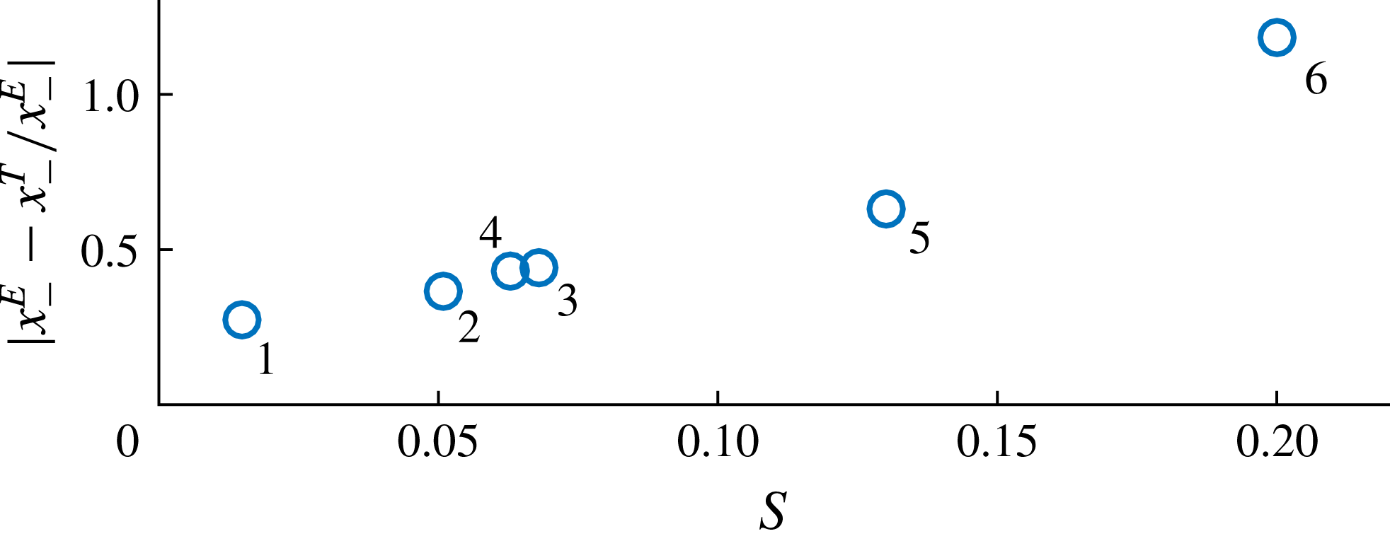
is evaluated for runs 1–6 in the final row of table 1. In figure 16, we have plotted the relative discrepancy between the final position of the negative flow front between theory,
 $x_{-}^{T}$
, and experiment,
 $x_{-}^{E}$
, against
 $S$
. The plot indicates a positive correlation between the value of (5.3) and the degree of discrepancy, indicating that the discrepancy is indeed due to a weakening of the assumption of hydrostatic pressure.
Scatter plot showing the correlation between the background strength parameter
 $S$
, as defined by (5.3), and the relative discrepancy between the final position of the negative flow front as predicted by the theory,
 $x_{-}^{T}$
, and the experimental data,
 $x_{-}^{E}$
, for runs 1–6. The positive correlation indicates that the weakening of the Dupuit approximation of predominantly horizontal flow, as measured by
 $S$
, is responsible for the discrepancy.
6 Geophysical applications
Background flow arises in geological aquifers as a consequence of hydrostatic pressure gradients from surface precipitation. This section applies the theoretical results to understand the general effects of background flow on both dissolved contaminants and injected fluid such as sequestered
 $\text{CO}_{2}$
.
6.1 Navajo Sandstone
As a case study, we consider the leaking of
 $\text{CO}_{2}$
-charged brine into the water-saturated Navajo Sandstone in North America. The brine originates from a much deeper formation saturated by
 $\text{CO}_{2}$
. The
 $\text{CO}_{2}$
-charged brine propagates from this aquifer through a permeable fault and, on its route to the surface, partially leaks into the Navajo Sandstone. The leaked fluid is subsequently advected tens of kilometres (e.g. Kampman et al.
Reference Kampman, Bickle, Becker, Assayag and Chapman2009) through this sandstone by a background flow of saturating water. Fluid samples taken from the reservoir through the depth of the aquifer near the fault indicate that
 $\text{CO}_{2}$
-charged brine spans the depth of the aquifer with a significant concentration gradient (Kampman et al.
Reference Kampman, Bickle, Maskell, Chapman, Evans, Purser, Zhou, Schaller, Gattacceca and Bertier2014). Measured or calculated parameters representing the aquifer and fluids are provided in table 2, with references provided in the caption.
Geophysical parameter estimates. The column for the Navajo case study lists specific values measured or calculated. The column for
 $\text{CO}_{2}$
storage lists generic representative values for reservoirs in which
 $\text{CO}_{2}$
sequestration may be applied.
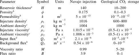
a Kampman et al. (Reference Kampman, Bickle, Maskell, Chapman, Evans, Purser, Zhou, Schaller, Gattacceca and Bertier2014).
b Kampman et al. (Reference Kampman, Bickle, Becker, Assayag and Chapman2009).
c Using the concentrations measured by Kampman et al. (Reference Kampman, Bickle, Maskell, Chapman, Evans, Purser, Zhou, Schaller, Gattacceca and Bertier2014) in conjunction with the tables of Dubacq, Bickle & Evans (Reference Dubacq, Bickle and Evans2013).
d Maskell (Reference Maskell2017).
The dissolved
 $\text{CO}_{2}$
and NaCl create a density difference of
 $\unicode[STIX]{x0394}\unicode[STIX]{x1D70C}\approx 12~\text{kg m}^{-3}$
and a viscosity ratio of
 $M=\unicode[STIX]{x1D707}_{2}/\unicode[STIX]{x1D707}_{1}=0.99$
. The flux ratio is
 $B=Q_{2}/Q_{1}\approx 3.9$
, indicating a significant role of background flow. Assuming that the input and ambient fluxes remain approximately constant, we apply the theoretical results of § 3. According to the theory, the interface between the injected and ambient fluids approaches an approximately horizontal interface along a height (3.9b
) given dimensionally by
 $$\begin{eqnarray}h_{H}=\frac{H}{1+MB}.\end{eqnarray}$$
For the values given above,
 $h_{H}\approx 0.2H\approx 30$
m. The brine is therefore predicted to occupy a region spanning one-fifth of the depth of the aquifer.
The corresponding prediction for the interstitial flow rate of the brine is
 $$\begin{eqnarray}u_{1}=\frac{Q_{1}}{\unicode[STIX]{x1D719}h_{H}}=(1+MB)\frac{Q_{1}}{\unicode[STIX]{x1D719}H},\end{eqnarray}$$
which is evaluated as
 $u_{1}\approx 4.2\times 10^{-7}~\text{m s}^{-1}\approx 13~\text{m yr}^{-1}$
. Based on this, the injected fluid is estimated to span the 20 km length of the Navajo Sandstone in approximately 1500 years. The prediction for the distance that the flow extends upstream against the background flow, as given by (3.11b
), has the dimensional form
 $$\begin{eqnarray}|x_{-}|=\frac{1}{2}\left[1-\left(1-\frac{1}{1+MB}\right)^{2}\right]\frac{\unicode[STIX]{x0394}\unicode[STIX]{x1D70C}gkH^{2}}{\unicode[STIX]{x1D707}_{2}Q_{2}}.\end{eqnarray}$$
This distance is evaluated as approximately 400 m. This value is consistent with the measurements of downhole fluid samples taken 100 m upstream of the fault (Kampman et al.
Reference Kampman, Bickle, Maskell, Chapman, Evans, Purser, Zhou, Schaller, Gattacceca and Bertier2014), indicating a limit to the extent of propagation of the brine against the groundwater flow. The result is also consistent with observations of bleaching of the exposed Entrada Sandstone related to previous inputs of
 $\text{CO}_{2}$
-rich brines (Wigley et al.
Reference Wigley, Kampman, Dubacq and Bickle2012). The bleaching occurs in the basal 20 m of the formation, extends less than 500 m upstream, and approximately 10 km downstream of the fault, which are consistent with our theoretical predictions.
6.2
 $\text{CO}_{2}$
injection

Next, we apply the results to investigate the effect of background flow on pure
 $\text{CO}_{2}$
injected into the subsurface for geological carbon storage. For this, we consider generic ranges of representative values for typical sandstone aquifers where geological carbon storage may be applied. These values are listed in the final column of table 2. For typical ranges of reservoir temperatures and fluid compositions, the
 $\text{CO}_{2}$
will be
 $M=5$
–20 times less viscous than the ambient water in the host rock. Given a representative input rate per unit width of
 $Q_{1}=10^{-4}~\text{m}^{2}~\text{s}^{-1}$
and a typical background flow rate of
 $Q_{2}=10^{-4}$
m, we estimate that
 $B$
can be of order unity. The case of no background flow,
 $B=0$
, may be more applicable to marine aquifers (such as the Sleipner project in the North Sea), for which precipitation cannot generate long-range hydrostatic imbalances. However, background flow can be driven in that case by poroelastic deformation due to the weight of the overlying rock. Below, we determine the magnitude of such motion necessary for an appreciable effect on the migration of
 $\text{CO}_{2}$
.
In accordance with the result of (3.10), the leading front of the
 $\text{CO}_{2}$
current is predicted to propagate in the direction of the background flow at a rate of
 $$\begin{eqnarray}u_{1}=M(1+MB)\frac{Q_{1}}{\unicode[STIX]{x1D719}H}\approx \frac{M^{2}Q_{2}}{\unicode[STIX]{x1D719}H}\approx M^{2}u_{2},\end{eqnarray}$$
where the last two approximations apply for
 $MB\gg 1$
. The injected fluid thus moves approximately
 $M^{2}$
times faster than the ambient fluid. The significant quadratic dependence on
 $M^{2}$
stems from the dual effect of the viscosity ratio for
 $M>1$
in both reducing the effective height of confinement of the current (given by (6.1)) and increasing the horizontal length of the convex similarity solution describing the injected current. For geological carbon storage, the
 $\text{CO}_{2}$
could travel as much as
 $M^{2}=400$
times faster than the background flow. A relatively small background flow may therefore be sufficient to have a significant impact on
 $\text{CO}_{2}$
spreading. Using a characteristic flow rate of the injected fluid of
 $u_{1}\approx 1.9\times 10^{-6}~\text{m s}^{-1}\approx 60~\text{m yr}^{-1}$
obtained from measurements of the
 $\text{CO}_{2}$
plume at Sleipner (Boait et al.
Reference Boait, White, Bickle, Chadwick, Neufeld and Huppert2012) and the viscosity ratio
 $M\approx 13$
, we determine that a background flow rate of just
 $u_{2}\approx u_{1}/M^{2}\approx 1.2\times 10^{-8}~\text{m s}^{-1}\approx 0.37~\text{m yr}^{-1}$
would be necessary to affect the migration of
 $\text{CO}_{2}$
significantly.
For the evolution of a parcel of
 $\text{CO}_{2}$
after its input ceases, we apply the predictions of the theory of § 4. The result of (4.1) predicts that the parcel of injected
 $\text{CO}_{2}$
is subsequently advected at the slower rate of a single factor of
 $M$
times the background flow rate,
 $u_{1}=Mu_{2}$
. The horizontal extent of the asymptotic similarity solution (4.11) arising under a background flow (4.12) has the dimensional form
 $$\begin{eqnarray}\unicode[STIX]{x0394}x(t)=\frac{2[M(M-1)Q_{2}{\mathcal{V}}t]^{1/2}}{\unicode[STIX]{x1D719}H},\end{eqnarray}$$
where
 ${\mathcal{V}}$
is the volume per unit width of fluid released. For illustrative values of
 $H=10$
m,
 $\unicode[STIX]{x1D719}=0.2$
,
 $M=10$
,
 $Q_{2}=10^{-5}~\text{m}^{2}~\text{s}^{-1}$
and
 ${\mathcal{V}}=10^{3}~\text{m}^{2}$
, (6.5) predicts that
 $\unicode[STIX]{x0394}x\approx 0.95\,t^{1/2}$
. This implies a horizontal extent of 280 m in 1 day, 5.3 km in 1 year and 170 km in
 $10^{3}$
years. It should be noted that this result assumes negligible residual trapping, an approximation that may apply in the case of a pure
 $\text{CO}_{2}$
parcel only if the aquifer contains an existing residual of
 $\text{CO}_{2}$
from a previous injection; a detailed evaluation of the effect of residual trapping is provided in the following subsection. The surface area of the interface between the injected
 $\text{CO}_{2}$
and the ambient water predicted by (6.5) may provide an ultimate constraint on the rate at which a parcel of
 $\text{CO}_{2}$
dissolves into the ambient water to become permanently secured.
6.3 Residual trapping
If the injectate is immiscible or only partially miscible in the ambient fluid, as applies to pure
 $\text{CO}_{2}$
injected into a saline aquifer, a certain proportion of fluid can be retained in the porous matrix as a residue trailing the parcel (Hesse et al.
Reference Hesse, Orr and Tchelepi2008). The primary effect of this trapping is to reduce the mass of the parcel of
 $\text{CO}_{2}$
over time. Let
 $R$
denote the proportion of the porous matrix occupied by residual
 $\text{CO}_{2}$
in the wake of the parcel; a typical value is
 $R\approx 0.2$
. Let
 $V(t)$
denote the volume of the pure
 $\text{CO}_{2}$
parcel. To investigate the effects of residual trapping, we model the loss to the capillary trail as being proportional to the height of the current multiplied by its leading-order rate of horizontal propagation,
 $$\begin{eqnarray}\dot{V}(t)\sim -Rh_{max}(t){\dot{x}}_{-}(t),\end{eqnarray}$$
where
 $h_{max}(t)\equiv \max _{x}[h(x,t)]$
. Using the asymptotic solution (4.20) to evaluate
 $h_{max}$
and (4.1) to evaluate
 ${\dot{x}}_{-}$
, we obtain the ordinary differential equation
 $$\begin{eqnarray}\dot{V}\sim -RH\left(\frac{2V}{\unicode[STIX]{x1D6FA}t}\right)^{1/2}\left[\frac{MQ_{2}}{\unicode[STIX]{x1D719}H}\right].\end{eqnarray}$$
On integrating this equation, we obtain the evolution of the volume of the parcel,
 $$\begin{eqnarray}V(t)=\left\{1-\frac{R}{\unicode[STIX]{x1D719}}\left[\frac{MQ_{2}t}{|M-1|V_{0}}\right]^{1/2}\right\}^{2}V_{0},\end{eqnarray}$$
where
 $V_{0}\equiv V(0)$
is the total volume of
 $\text{CO}_{2}$
input. This analytical result yields an efficient means to assess the effect of capillary retention for mobilisation of a packet of sequestered
 $\text{CO}_{2}$
over time. Setting
 $V=0$
in (6.8) yields the total time
 $t_{res}$
and horizontal distance
 $x_{res}=x_{\pm }$
at which the
 $\text{CO}_{2}$
becomes fully residually trapped, given by
 $$\begin{eqnarray}t_{res}=\frac{|M-1|}{M}\frac{\unicode[STIX]{x1D719}^{2}}{R^{2}}\frac{V_{0}}{Q_{2}},\quad x_{res}=\frac{|M-1|\unicode[STIX]{x1D719}V_{0}}{R^{2}H}\end{eqnarray}$$
respectively. Using the values for our numerical example given in § 6.2 above, we evaluate
 $t_{res}\approx 3$
yr, which indicates that a packet of
 $\text{CO}_{2}$
will become fully trapped by capillary retention after a few years. It is interesting that the distance propagated by the parcel,
 $x_{res}$
, given by (6.9b
) does not depend on the background flux
 $Q_{2}$
. The ‘favourable’ cancellation of
 $Q_{2}$
in deriving this result is caused by the coincidence that a faster background flow rate simultaneously increases both the rate of propagation of the parcel and the rate of mass loss. For our illustrative parameter values, the total distance propagated by the parcel is
 $x_{res}\approx 4.5$
km.
Residual trapping is likely to be a significant effect for a first-time finite (post-injection) release of
 $\text{CO}_{2}$
. It should be noted, however, that it does not occur in the case of a constant-flux input (§ 3), because, in that case, the current only grows (
 $\unicode[STIX]{x2202}h/\unicode[STIX]{x2202}t>0$
) and thus cannot leave a trail. This case may be of greater relevance to industrial-scale
 $\text{CO}_{2}$
, for which the aim would be to use the full aquifer for storage, as opposed to releasing a finite volume that occupies a relatively small proportion of the total available storage space. Residual trapping is also not relevant if the injectate is miscible (
 $R=0$
), as applies to the migration of dissolved
 $\text{CO}_{2}$
or contaminants through aquifers.
6.4 Model applicability
We end by summarising the applicability of our theoretical results. Three sources of additional physical effects not included in our model include those identified by our laboratory study, namely the possible role of vertical stresses, as measured by the parameter (5.3), the role of time-dependent variations in fluxes caused by the gradual accumulation of less viscous fluid in the reservoir, and the effect of localised patches of fluid left in the wake of the parcel inside local regions of low permeability. Perhaps the primary limitation of the solutions we describe is as a model for the localised continuous injection of
 $\text{CO}_{2}$
at a point source. In such cases, it is permissible for the
 $\text{CO}_{2}$
to expand to fill the depth of the aquifer at the injection site because the ambient fluid can flow laterally around the injection zone, a feature that cannot occur for the infinite line source we have assumed. The input of brine into the Navajo Sandstone is introduced through a linear fault along a length of approximately 2 km. We anticipate that the flow near the input may approximate that of a linear source, but, for scales much larger than the fault, the flow will approach an asymptotic regime that is effectively fed by a point source. Some lateral spreading of the flow will also occur under gravity in the direction perpendicular to the background flow, which is not addressed by our analysis. Other three-dimensional effects may stem from the fact that the fault is aligned at an angle to the prevailing background flow, as well as being partially sealing. For the finite-volume release, we anticipate that the asymptotic regimes we describe do also apply to leading order in the case of a three-dimensional parcel released into a linear background flow because the control of the flow deformation by the background flow will dominate at long times over lateral spreading of the parcel under gravity. An exploration of these three-dimensional phenomena may provide interesting directions for future analysis.
7 Conclusions
We have developed a theory describing regimes of contaminant transport in geological reservoirs by a background flow, tested its predictions using experimental data, and applied the results to assess the significance of background flow in natural examples. The results show that background flow and far-field asymmetries have dominant controls on released fluids in typical subsurface environments.
For a continuous injection along a line source into the interior of an aquifer, the injection initially flows symmetrically, with equal parts flowing upstream and downstream. Asymmetry quickly arises as the effects of a background flow or, in the case of no background flow, the asymmetries in the far-field boundary conditions take hold. A dedicated analysis of the special regimes arising for the case of no imposed background flow was conducted, which provides a model of the injection into an aquifer bounded between a sealing fault and a permeable fault. Fluid was found to propagate predominantly towards the permeable fault as
 $t$
and, in this direction, ultimately approaches the equivalent asymptotic regimes found previously for a one-sided injection. The component flowing towards the sealing fault instead forms a self-similar flow growing as
 $t^{1/2}$
with a prefactor dependent on the viscosity ratios. This growth predicts that the entire aquifer ultimately becomes saturated by the injected fluid, but with the region between the input and the sealing fault taking considerably longer. The filling towards the sealing fault occurs more slowly when the injected fluid is less viscous compared with the ambient because of a dominant effect of the stresses associated with mobilising a return flow of ambient fluid in order to conserve mass. In the limit of small injectate viscosity, the
 $t^{1/2}$
similarity solution contains a boundary layer at the flow front in which the injectate viscosity ultimately intervenes to constrain the rate of propagation.
Background flow was found to cap a continuously injected current below a depth given by (6.1). The regimes arising downstream of the input are equivalent to those of a one-sided injection into a shallower aquifer with the effective thickness (6.1). Upstream, the flow approaches a steady state of finite extent (6.3), contrasting with the indefinite
 $t^{1/2}$
expansion occurring in the case of no background flow. For injected fluid less viscous than the ambient fluid, the background flow drives an injected fluid at a rate that can be considerably faster than the background flow rate itself. That contribution is equal to the speed of the background flow rate multiplied by the square of the viscosity ratio (6.4), a factor which can be as high as 400 for
 $\text{CO}_{2}$
injected into a saline aquifer.
For the release of a parcel of fixed volume, we found that a background flow advects the parcel as a whole at a rate given by the background flow speed multiplied by the viscosity ratio. Moving the governing equations into the frame of the parcel revealed that background flow not only advects the parcel as a whole but also controls the deformation of the parcel itself. The phenomenon occurs as a consequence of contrasts in the rates at which the two fluid species are driven by the background pressure gradient. It generally provides the dominant control on deformation. The only exception is when the injected and ambient fluids have equal viscosity, in which case the gravitational dynamics uniquely remains dominant. In all other cases, gravitational spreading becomes negligible. The leading-order equation describing the deformation due to the background pressure gradient is a nonlinear wave equation with a height-dependent advective prefactor. Similarity solutions to this equation show that the asymptotic extent under this effect grows as
 $t^{1/2}$
. The rate of horizontal growth is faster than occurs under gravity alone (or in the case of equal viscosities), for which the parcel relaxes as
 $t^{1/3}$
. The self-similar asymptotic profile contains a triangular cross-section with a steep shock at the downstream or upstream flow front for an injectate that is more or less viscous than the ambient, respectively. Wave breaking at the shock is suppressed by a short region in which gravity intervenes to prevent the overturning of the interface. For a parcel more viscous than the ambient, there is an ‘optimal’ rate of stretching of the horizontal extent when the injected fluid is exactly twice as viscous as the ambient.
We developed new analytical results describing the asymptotic effects of capillary retention on the evolution of an immiscible or partially immiscible fluid parcel in a porous medium, such as applied to pure
 $\text{CO}_{2}$
released into a saline aquifer. The analysis yields analytical expressions for the volume of the parcel over time, and the total time and distance by which a parcel of
 $\text{CO}_{2}$
becomes fully retained. Interestingly, even though the analysis depends on the asymptotic regimes arising under a driving background pressure, the distance propagated by the parcel in that time, given by (6.9b
), is completely independent of the background flow rate.
Our experimental data showed generally good agreement with the theoretical predictions. Some discrepancies at the upstream flow front were found to correlate with a dimensionless parameter grouping (5.3) that is larger for larger background fluxes
 $Q_{2}$
, and indicated that the discrepancies can be attributed to the significance of vertical stresses caused by large interfacial gradients near the upstream flow front. Finite-volume experiments show that the parcel leaves a trail of residual patches of fluid as it propagates. We attribute this effect to pore-scale trapping of the injected fluid in localised regions of small permeability within the heterogeneous pore structure.
The results were applied to geological examples, demonstrating their determination of the relative significance of background flow, the flow rate induced by background flow, an assessment of the minimum background flow necessary to have a significant impact, the time scales on which its effects have an impact, and the effects of capillary retention. We considered both a case study of the contamination of the Navajo Sandstone by a source of dissolved
 $\text{CO}_{2}$
-charged brine and general examples of the migration of pure
 $\text{CO}_{2}$
following its injection into a saline aquifer. In the former case, background flow advects the brine at approximately
 $10~\text{m yr}^{-1}$
and occupies an effective depth of confinement in the lower fifth of the reservoir. The prediction for the distance propagated against the background flow (400 m) is consistent with the extent of observed bleaching of exposed sections of the formation. For geological carbon storage, the significantly smaller viscosity of the injected fluid compared with the ambient water can have considerable implications for the effects of a background flow. The injected fluid is predicted to propagate as much as 400 times faster than the ambient fluid during the input stage or 20 times faster after the input ceases. These results indicate that background flow can have a strong independent control of injected
 $\text{CO}_{2}$
and can play a vitally important role in geological environments where
 $\text{CO}_{2}$
sequestration may be applied.
Acknowledgements
A.S.D.M. acknowledges support by EPSRC for a doctoral training grant and from NERC under Highlight grant NE/N016084/1. K.A.D. was supported by a CCS Innovation grant provided by DECC. We are grateful to C. Hitch and D. Page-Croft for making necessary adjustments to our laboratory apparatus.
Supplementary movie
A supplementary movie is available at https://doi.org/10.1017/jfm.2017.501.
Appendix A. Numerical method for time integration
This appendix provides the details of our numerical method used to solve the time-dependent equations (2.13)–(2.17). We first recast the equations into a new coordinate system in which the two flow fronts and the point of input are temporally fixed, then apply a partially implicit finite-difference scheme to the resulting system. The rescaling eliminates any numerical issues with the transition to zero thickness at the flow fronts (2.16a
) and (2.17a
), and additionally allows the numerical grid size to scale directly with the current, thereby resolving the large interfacial gradients associated with the early-time
 $t^{2/3}$
similarity solution (3.1) used for initialisation. Similar numerical schemes were used in the previous analyses of Pegler et al. (Reference Pegler, Huppert and Neufeld2014a
,Reference Pegler, Huppert and Neufeld
b
), wherein further validation by comparison with asymptotic similarity solutions and laboratory experiments was provided.
For the case of a continuous input, we apply the transformation
 $$\begin{eqnarray}X=\left\{\begin{array}{@{}ll@{}}x/|x_{-}(t)|, & \text{for}~x_{-}(t)\leqslant x\leqslant 0,\\ x/x_{+}(t), & \text{for}~0<x\leqslant x_{+}(t),\end{array}\right.\end{eqnarray}$$
which maps
 $x_{-}$
 $(t)$
to the fixed point
 $X=-1$
,
 $x_{+}$
 $(t)$
to the fixed point
 $X=1$
, and the source point
 $x=0$
to the fixed point
 $X=0$
.
In terms of the new coordinate system
 $(X,t)$
, for
 $X>0$
, (2.13) becomes
 $$\begin{eqnarray}h_{t}-\frac{{\dot{x}}_{+}}{x_{+}}Xh_{X}=-\frac{1}{x_{+}}\left(\frac{MQ(X,t)-x_{+}^{-1}(1-h)h_{X}}{Mh+(1-h)}\right)_{X},\end{eqnarray}$$
where the
 $X$
and
 $t$
subscripts denote partial derivatives. A similar equation with
 $|x_{-}|$
in place of
 $x_{+}$
and
 ${\dot{x}}_{-}$
in place of
 ${\dot{x}}_{+}$
applies for
 $X<0$
. Condition (2.14) becomes
 $$\begin{eqnarray}x_{+}^{-1}h_{X}(0_{+},t)-|x_{-}|^{-1}h_{X}(0_{-},t)=(M-h(0,t)^{-1})I(t),\end{eqnarray}$$
 $$\begin{eqnarray}h(1,t)=0,\quad {\dot{x}}_{+}=M[I(t)+B]-x_{+}^{-1}h_{X}(1,t),\end{eqnarray}$$
 $$\begin{eqnarray}\hspace{-22.50003pt}h(-1,t)=0,\quad {\dot{x}}_{-}=MB-|x_{-}|^{-1}h_{X}(-1,t).\end{eqnarray}$$
We now discretise the system. Let
 $h_{i}^{k}$
denote the thickness at the
 $i$
th spatial node and
 $k$
th time step,
 $h(X_{i},t_{k})$
, where
 $X_{i}$
is a nodal grid with
 $X_{1}=-1$
,
 $X_{S}=0$
and
 $X_{N}=1$
, and
 $t_{k}$
is the time at the
 $k$
th time step. Here,
 $i=S$
denotes the source node
 $X_{S}=0$
. The nodal grid
 $X_{i}$
is imposed in two regions: one region is upstream of the input point,
 $1\leqslant i<S$
, with step size
 $\unicode[STIX]{x1D6FF}X_{-}$
; the second is downstream of the input point,
 $S<i\leqslant N$
, for which the step size is
 $\unicode[STIX]{x1D6FF}X_{+}$
. For simplicity, the step size in the two domains was typically taken as equal,
 $\unicode[STIX]{x1D6FF}X=\unicode[STIX]{x1D6FF}X_{-}=\unicode[STIX]{x1D6FF}X_{+}$
.
For every node
 $i$
(other than those where a boundary condition is applied, namely 1,
 $S$
and
 $N$
), we applied a semi-implicit centred finite-difference scheme to approximate the spatial derivatives in (A 2). Thus, we rewrite (A 2) as
 $$\begin{eqnarray}\unicode[STIX]{x1D6FF}th_{t}=\unicode[STIX]{x1D6FC}(h)\unicode[STIX]{x1D6FF}X^{2}h_{XX}+\unicode[STIX]{x1D6FD}(h,h_{X})(2\unicode[STIX]{x1D6FF}X)h_{X},\end{eqnarray}$$
where
 $\unicode[STIX]{x1D6FF}t$
is the time step,
 $\unicode[STIX]{x1D6FF}X$
is the length step and
 $$\begin{eqnarray}\displaystyle & \displaystyle \unicode[STIX]{x1D6FC}(h)=\frac{\unicode[STIX]{x1D6FF}t}{\unicode[STIX]{x1D6FF}X^{2}x_{+}^{2}}\left[\frac{Mh(1-h)}{Mh+(1-h)}\right], & \displaystyle\end{eqnarray}$$
 $$\begin{eqnarray}\displaystyle & \displaystyle \unicode[STIX]{x1D6FD}(h,h_{X})=\frac{\unicode[STIX]{x1D6FF}t}{2\unicode[STIX]{x1D6FF}Xx_{+}}\left[\frac{M(M-B-2Mh-h^{2}+Mh^{2}h_{X}/x_{+})}{[\!Mh+(1-h)\! [^{2}}+{\dot{x}}_{+}X\right], & \displaystyle\end{eqnarray}$$
and apply the difference approximations
 $$\begin{eqnarray}\displaystyle \displaystyle h_{X} & {\approx} & \displaystyle (h_{i+1}^{k+1}-h_{i-1}^{k+1})/(2\unicode[STIX]{x1D6FF}X),\end{eqnarray}$$
 $$\begin{eqnarray}\displaystyle \displaystyle h_{XX} & {\approx} & \displaystyle (h_{i+1}^{k+1}-2h_{i}^{k+1}+h_{i-1}^{k+1})/(\unicode[STIX]{x1D6FF}X^{2}),\end{eqnarray}$$
 $$\begin{eqnarray}\displaystyle \displaystyle h_{t} & {\approx} & \displaystyle (h_{i}^{k+1}-h_{i}^{k})/\unicode[STIX]{x1D6FF}t.\end{eqnarray}$$
A nonlinearity in derivatives arises because of the
 $h_{X}$
term in
 $\unicode[STIX]{x1D6FD}$
given in (A 8). In order to maintain a numerically linear discretised problem, we evaluate the
 $h_{X}$
term in
 $\unicode[STIX]{x1D6FD}$
using the current time step
 $k$
. This results in a partially implicit scheme, which is satisfactorily stable in practice. With the discretisations of (A 9) substituted, equation (A 6) becomes
 $$\begin{eqnarray}h_{i}^{k+1}-h_{i}^{k}=\unicode[STIX]{x1D6FC}_{i}^{k}(h_{i+1}^{k+1}-2h_{i}^{k+1}+h_{i-1}^{k+1})+\unicode[STIX]{x1D6FD}_{i}^{k}(h_{i+1}^{k+1}-h_{i-1}^{k+1}),\end{eqnarray}$$
where
 $\unicode[STIX]{x1D6FC}_{i}^{k}=\unicode[STIX]{x1D6FC}(h_{i}^{k})$
and
 $\unicode[STIX]{x1D6FD}_{i}^{k}=\unicode[STIX]{x1D6FD}[h_{i}^{k},(h_{X})_{i}^{k}]$
. First-order approximations can be applied to discretise (A 3), which becomes
 $$\begin{eqnarray}\frac{1}{x_{+}}\left(\frac{h_{i+1}^{k+1}-h_{i}^{k+1}}{\unicode[STIX]{x1D6FF}X}\right)-\frac{1}{|x_{-}|}\left(\frac{h_{i}^{k+1}-h_{i-1}^{k+1}}{\unicode[STIX]{x1D6FF}X}\right)=\left(M-\frac{1}{h_{i}^{k}}\right)I(t),\end{eqnarray}$$
and conditions (A 4a ) and (A 5a ) become
 $$\begin{eqnarray}h_{1}=h_{N}=0.\end{eqnarray}$$
Equations (A 12)–(A 14) form a tridiagonal linear system for
 $h_{i}^{k+1}$
, which we solved using Matlab’s internal linear inversion routine.
For the solutions of § 4, the source is abruptly ceased at
 $t=V$
. Beyond that time, there is no need to fix the position of the input. For this case, we applied a modified slightly simpler rescaling of the flow to a single fixed domain via the alternative rescaling
 $$\begin{eqnarray}X^{\prime }=\frac{x-x_{-}(t)}{x_{+}(t)-x_{-}(t)},\end{eqnarray}$$
which maps the current onto the fixed interval of
 $X^{\prime }$
given by
 $[0,1]$
. The transformed system is omitted here for brevity. A transfer of the solution to the new nodal representation over a regular grid of
 $X^{\prime }$
at
 $t=V$
was conducted using a cubic spline.
Appendix B. Boundary-layer structure for small injectate viscosity
This appendix analyses the boundary-layer structure underlying the self-similar flow towards the sealed section of a geological reservoir (the case of zero background flow illustrated in figure 5), as described by (3.5) and (3.6), in the limit of small injectate viscosity,
 $\unicode[STIX]{x1D716}\equiv M^{-1}\rightarrow 0$
. In terms of the more convenient variables
 $(\unicode[STIX]{x1D709},\unicode[STIX]{x1D709}_{N})\equiv \unicode[STIX]{x1D716}^{1/2}(\unicode[STIX]{x1D702},\unicode[STIX]{x1D702}_{N})$
, (3.5) can be expressed as
 $$\begin{eqnarray}-\frac{1}{2}\unicode[STIX]{x1D709}h^{\prime }=\left[\frac{h(1-h)h^{\prime }}{h+\unicode[STIX]{x1D716}(1-h)}\right]^{\prime }\end{eqnarray}$$
and conditions (3.6a,b ) as
 $$\begin{eqnarray}h(0)=1,\quad h(-\unicode[STIX]{x1D709}_{N})=0,\quad h^{\prime }(-\unicode[STIX]{x1D709}_{N})={\textstyle \frac{1}{2}}\unicode[STIX]{x1D716}\unicode[STIX]{x1D709}_{N}.\end{eqnarray}$$
We first seek a regular leading-order expansion in the limit
 $\unicode[STIX]{x1D716}\rightarrow 0$
under the assumption that
 $h=O(1)$
. In this limit, equation (B 1) reduces to
 $$\begin{eqnarray}-{\textstyle \frac{1}{2}}\unicode[STIX]{x1D709}h^{\prime }\sim [(1-h)h^{\prime }]^{\prime },\end{eqnarray}$$
which describes the motion of the interface under the assumption that it is resisted predominantly by the ambient flow. By integrating (B 3) numerically subject to (B 2) using a similar scheme to that used for (3.5), we obtain the outer solution shown as a dotted red curve in figure 5. For
 $h\rightarrow 0$
, equation (B 3) reduces asymptotically to
 $$\begin{eqnarray}-\frac{1}{2}\unicode[STIX]{x1D709}h^{\prime }\sim h^{\prime \prime }\quad \text{and hence}\quad h\sim \frac{2K}{\sqrt{\unicode[STIX]{x03C0}}}\,\text{erf}\left(\frac{\unicode[STIX]{x1D709}}{2}\right)\sim \frac{K\text{e}^{-\unicode[STIX]{x1D709}^{2}/4}}{-\unicode[STIX]{x1D709}}\end{eqnarray}$$
as
 $\unicode[STIX]{x1D709}\rightarrow -\infty$
, where
 $\text{erf}$
is the error function,
 $K$
is a constant of integration and we have used the leading-order asymptotic approximation for
 $\text{erf}$
in the limit of large argument. To find where this outer solution predicts its own asymptotic inconsistency, it should be noted that the term of
 $O(\unicode[STIX]{x1D716})$
in the denominator of (B 1) becomes important wherever
 $h=O(\unicode[STIX]{x1D716})$
, or, using (B 4b
), for
 $-\unicode[STIX]{x1D709}=O(\unicode[STIX]{x1D706})$
, where
 $\unicode[STIX]{x1D706}\equiv [\log (1/\unicode[STIX]{x1D716})]^{1/2}$
. This observation motivates a leading-order asymptotic approximation for the extent given by
 $\unicode[STIX]{x1D709}_{N}=a\unicode[STIX]{x1D706}$
, where
 $a$
is a constant to be determined.
The predicted importance of the
 $O(\unicode[STIX]{x1D716})$
term in (B 1) indicates the existence of a boundary layer near
 $-\unicode[STIX]{x1D709}_{N}$
in which the viscosity of the injectate becomes leading order. To determine the leading-order reduction of (B 1) near
 $-\unicode[STIX]{x1D709}_{N}$
, we re-express it in terms of the scaled inner coordinates
 $$\begin{eqnarray}z=\unicode[STIX]{x1D706}^{-1}(\unicode[STIX]{x1D709}_{N}+\unicode[STIX]{x1D709}),\quad h=MF(z).\end{eqnarray}$$
In terms of these variables, (B 1) and (B 2b,c ) become
 $$\begin{eqnarray}-aF^{\prime }=\left(\frac{FF^{\prime }}{F+1}\right)^{\prime },\quad F(0)=0,\quad F^{\prime }(0)=\frac{1}{2}a,\end{eqnarray}$$
where higher-order terms have been neglected and a prime here implies differentiation with respect to
 $z$
. On integrating (B 6), we obtain the inner solution
 $$\begin{eqnarray}F=-1+\text{e}^{(a/2)z}\quad \text{or}\quad h=M[-1+\text{e}^{(a/2)\unicode[STIX]{x1D706}^{-1}(\unicode[STIX]{x1D709}_{N}+\unicode[STIX]{x1D709})}]\end{eqnarray}$$
when expressed back in terms of the outer coordinates using (B 5).
Finally, we match (B 4) and (B 7). By comparing the logarithms of the reduced forms of (B 4b
) and of the inner solution (B 7b
) in the intermediate region
 $\unicode[STIX]{x1D706}\gg -\unicode[STIX]{x1D709}\gg 1$
(the latter being given by neglecting just the
 $-1$
term), we deduce that
 $a=2$
and hence
 $\unicode[STIX]{x1D709}_{N}=2\unicode[STIX]{x1D706}$
, from which (3.7) follows. The inner solution (B 7) with
 $a=2$
is plotted as a dashed curve in figure 5 and is confirmed to match to the flow front consistently.