

1 Introduction
In this paper we employ simultaneous laryngoscopy and laryngeal ultrasound (SLLUS; Moisik et al. Reference Moisik, Esling, Bird and Lin2011) to assess laryngeal mechanisms involved in producing Mandarin tones. Electromyographic (EMG) research by Sagart et al. (Reference Sagart, Hallé, de Boysson-Bardies and Arabia-Guidet1986), Erickson (Reference Erickson1993, Reference Erickson2011), and Hallé (Reference Hallé1994) has shown indirectly that changes in larynx height do occur during tone production in Mandarin and Thai, but direct observation of larynx height or larynx state has not been pursued to the same extent. This may be partly due to the lack of real-time techniques available to observe and measure these factors in the execution of tone (concerning larynx height, see Honda Reference Honda2004). Understanding how glottal pitch can be influenced by larynx height and changes in larynx state provides us with a basis to better model the linguistic role of the connection between the systems governing vocal fold oscillation and the rest of the vocal tract (Honda Reference Honda, Bell-Berti and Raphael1995).
The basic role of larynx height in the execution of tone is complicated by the relationship of larynx height to the state of the larynx: constriction of the supra-glottal laryngeal structures is facilitated by raising the larynx (Edmondson & Esling Reference Edmondson and Esling2006) and inhibited by lowering the larynx. Laryngeal constriction can have substantial consequences on the dynamics of the vocal folds by changing their configuration and mechanical relationship to other laryngeal structures such as the ventricular folds (Laver Reference Laver1980). The connection between larynx height and state, however, has not been fully explored in the context of a tone language. Therefore, this study aims to explore these issues through the application of the SLLUS technique to Mandarin.
We present evidence that larynx height and laryngeal constriction are active in Mandarin tone production and serve a facilitating or compensatory role to the primary musculature responsible for pitch regulation. Our findings generally complement those of Sagart et al. (Reference Sagart, Hallé, de Boysson-Bardies and Arabia-Guidet1986) and Hallé (Reference Hallé1994) that larynx height positively correlates with f0 in Mandarin tones; however, we observe that the action of the laryngeal constrictor mechanism and its relation to larynx height complicates this analysis. Beyond the widely attested observation (Honda et al. Reference Honda, Hirai, Masaki and Shimada1999) that larynx lowering is a correlate of pitch lowering, we find that larynx raising in conjunction with laryngeal constriction can also yield low pitch, which is precisely the mechanism predicted by Lindqvist-Gauffin (Reference Lindqvist-Gauffin1972). The relationship between laryngeal constriction and larynx height is clearly described in physiological terms by Fink (Reference Fink1974, Reference Fink1975) and, in phonetic terms, it is extensively documented in Esling (Reference Esling1996), Esling & Harris (Reference Esling2005), Edmondson & Esling (Reference Edmondson and Esling2006), Esling, Zeroual & Crevier-Buchman (Reference Esling, Zeroual and Crevier-Buchman2007), Lindblom (Reference Lindblom2009), and Esling & Moisik (Reference Esling, Moisik, Gibbon, Hirst and Campbell2012), inter alia.
We also observe that both larynx raising and lowering mechanisms are employed by a single participant to accomplish different types of tone targets, largely depending on rate of pitch change. Our proposal is that, in addition to f0 regulation via cricothyroid joint rotation, f0 can also be manipulated through laryngeal constriction and larynx height. These mechanisms change the vertical relationship of the laryngeal structures, the effect of which is to change the relationship between the vocal folds and the ventricular folds and a corresponding change in vocal fold dynamics.
An important feature of our study is the use of the SLLUS technique to study both larynx height and larynx state at the same time. The two techniques involved, laryngoscopy and laryngeal ultrasound, complement each other: laryngoscopy is ideal for obtaining information about the state of the larynx, but it only provides a limited impression of larynx height, whereas laryngeal ultrasound can be used to quantify changes in larynx height, although it is not an optimal means to study laryngeal state. The simultaneous use of these two techniques provides us with a more complete picture of laryngeal behaviour than one could obtain with either technique independently or with indirect measurements using EMG. Furthermore, larynx height has been one of the more difficult vocal tract parameters to measure (Honda et al. Reference Honda, Hirai, Masaki and Shimada1999: 402; Honda Reference Honda2004), and our approach illustrates how ultrasound can serve as a convenient and robust tool to quantify larynx height.
Larynx height was quantified by applying optical flow analysis (Horn & Schunck Reference Horn and Schunck1981) to the laryngeal ultrasound data. Optical flow analysis creates discrete velocity fields that represent movement between pairs of frames and these can be used to study the kinematic properties of objects observed in video data. The optical flow algorithm employed in this study is a simple, custom, block-wise cross-correlation-based assessment of movement registered in pairs of contiguous frames (discussed at length in Section 3). Very little research has been done which employs optical flow analysis to study video data of speech processes (although, see Barbosa, Yehia & Vatikiotis-Bateson Reference Barbosa, Yehia and Vatikiotis-Bateson2008; Lammert, Proctor & Narayanan Reference Lammert, Proctor and Narayanan2010; Narayanan et al. Reference Narayanan, Bresch, Ghosh, Goldstein, Katsamanis, Kim, Lammert, Proctor, Ramanarayanan and Zhu2011: 839), and optical flow has not previously been applied to ultrasound data in speech research.
1.1 Previous laryngeal ultrasound research and measurement of larynx height
There is not much precedent for the use of laryngeal ultrasound in speech research, although a handful of vocal fold vibration studies have been attempted in the past (e.g. Mensch Reference Mensch1964, Hertz, Lindström & Sonesson Reference Hertz, Lindström and Sonesson1970, Holmer, Kitzing & Lindström Reference Holmer, Kitzing and Lindström1973), and more recently researchers have used colour Doppler imaging to study the mucosal wave of the vocal and ventricular folds (Shau et al. Reference Shau, Wang, Hsieh and Hsiao2001, Tsai, Shau & Hsiao Reference Tsai, Shau and Hsiao2004). The use of ultrasound to image the larynx under semi-static conditions and during movement is common enough in the clinical setting, and there are several publications concerning normal and pathological laryngeal physiology and development (e.g. Harries et al. Reference Harries, Hawkins, Hacking and Hughes1998, Sonies, Chi-Fishman & Miller Reference Sonies, Chi-Fishman, Miller and Bronwyn2002, Loveday Reference Loveday2003, Rubin et al. Reference Rubin, Lee, McGuinness, Hore, Hill and Berger2004, Jadcherla et al. Reference Jadcherla, Gupta, Stoner, Coley, Wiet and Shaker2006).
Laryngeal ultrasound has not yet been applied to the study of larynx height. Previous attempts at measuring larynx height employ techniques that have drawbacks not encountered with laryngeal ultrasound. For example, thyro-umbrometry (e.g. Ewan & Krones Reference Ewan and Krones1974, Sprouse, Solé & Ohala Reference Sprouse, Solé and Ohala2010) tracks the movement of the laryngeal prominence from video of a back-lit subject. The obvious constraint on this technique is the necessity for the participant to have a large laryngeal prominence so that the movement of the larynx can be easily tracked. Another problem with the thyro-umbrometer is that, by only using the external appearance of the larynx, it is unclear if the movement of the laryngeal prominence is purely associated with changes in larynx height, or if it is attributable to rotation of the thyroid cartilage about the cricothyroid joint. The arc swept out by thyroid rotation will be large at the laryngeal prominence because it is far from the axis of rotation (the cricothyroid joint), and hence the influence of rotation could be considerable.
EMG can be used to infer information about laryngeal movements by means of muscle activation patterns. This approach can be used to indirectly infer the role of larynx height in the production of tone and the linguistic use of pitch (e.g. Simada & Hirose Reference Simada and Hirose1970, Sawashima, Kakita & Hiki Reference Sawashima, Kakita and Hiki1973, Collier Reference Collier1975, Sagart et al. Reference Sagart, Hallé, de Boysson-Bardies and Arabia-Guidet1986, Erickson Reference Erickson1993, Hallé Reference Hallé1994). Measurement of muscle activation alone, however, does not uniquely determine larynx height since the system at large is characterized by agonist-antagonist relationships, which means that high activation does not guarantee that the agonist effect of a muscle is being observed (e.g. see Vilkman et al. Reference Vilkman, Sonninen, Hurme and Körkkö1996 regarding the complex relationship between laryngeal muscles and f0). Thus, without external confirmation of changes in larynx height, EMG only offers suggestive information that the larynx is indeed moving in the supposed direction of the corresponding muscle force vector.
Standard MRI provides a very direct method of determining absolute larynx height (e.g. Honda et al. Reference Honda, Hirai, Masaki and Shimada1999, Nissenbaum et al. Reference Nissenbaum, Kirsch, Halle, Kobler, Curtin and Hillman2002), but it is an expensive technique with limited accessibility and cannot provide high resolution in the time domain since it requires static postures to be maintained for several seconds in order to produce images with clear enough structural resolution for measurements to be obtained (Whalen Reference Whalen2004). The temporal resolution can be improved by restricting imaging to a single plane (e.g. mid-sagittal), but the frame rates do not yet compare with those achievable by means of ultrasound. More recently, thanks to various improvements in MRI technology, real-time MRI (rtMRI) is becoming a reality. Bresch et al. (Reference Bresch, Kim, Nayak, Byrd and Narayanan2008) report that the system can operate at 5–50 frames per second, although image resolution is low. For example, Narayanan et al. (Reference Narayanan, Bresch, Ghosh, Goldstein, Katsamanis, Kim, Lammert, Proctor, Ramanarayanan and Zhu2011: 838) report that, for a 5 mm width midsagittal scan slice at a (reconstructed) frame rate of 23.18 frames per second, a resolution of 68 × 68 pixels (2.9 × 2.9 mm) is attainable. In general, however, another drawback of MRI is scanner noise, which compromises the quality of acoustic data.
We submit the claim that laryngeal ultrasound is a good solution to the problem of obtaining information about larynx height. Unlike thyro-umbrometry laryngeal ultrasound is not strongly dependent on any one feature of participant anatomy to obtain results, and thus it is applicable to a wider set of participants (e.g. those without large or obvious laryngeal prominences). Furthermore, since an entire plane of motion is imaged with laryngeal ultrasound, thyroid rotation will constitute only a part of the total motion of the larynx. Thus, thyroid rotation will have less of a confounding effect on larynx-height measurement in the context of laryngeal ultrasound than it will in the context of a technique such as thyro-umbrometry, which solely tracks thyroid notch movement. Unlike EMG, laryngeal ultrasound is non-invasive and provides a direct measurement of larynx height, and unlike MRI, the temporal resolution in laryngeal ultrasound is high, and it is easy to achieve the standard 30 frames per second with the technique.
2 Methodology
Modern Standard Chinese is chosen as the subject of study since its tone system is relatively well understood, it is easy to find fluent speakers, and the set of tones is relatively small and therefore more tractable to describe. Mandarin Chinese has five tones – four basic tones and a neutral tone. On Yuen Ren Chao's scale of five pitch levels (Chao Reference Chao1968), they have the values of 55 (high level), 35 (mid rising), 213 (falling rising) and 51 (high falling), respectively (Lin Reference Lin2001: 44). These values are, however, found on citation tones and in pre-pausal position. When followed by another tone within the prosodic domain of the foot, the phonetic values of these tones alter via tone sandhi rules (Lin Reference Lin, Xu and Zhong2007).Footnote 1 The four tones in pre-pausal position have varied durations. Tone 3 (T3) is the longest, followed by Tone 2 (T2), which in turn is followed by Tone 1 (T1). Tone 4 (T4) is the shortest (Howie Reference Howie1976). However, when followed by another tone within the same prosodic domain, these tones (or rather, the syllables carrying them) have more or less the same length (Wang & Wang Reference Wang and Wang1993). Indeed, in non-final position, the duration of the tone is a function of the prosodic position rather than tone membership (Shen Reference Shen1990a, Reference Shenb). For this study, we have restricted our attention to just the monosyllabic, citation form of the tones so as to focus on canonical effects of larynx height and state and avoid complicating factors such as tone sandhi.
Three participants volunteered to take part in the research project. Two of them are native speakers, and they will be referred to throughout as Participant-M (male) and Participant-F (female). We also obtained elicitations from a highly trained phonetician and additional-language user of Mandarin, whom we will refer to as Participant-P, and his productions were judged by several native Mandarin speakers (including the two other participants in this study) to be highly natural sounding. We consider his data to represent careful phonetic productions of the tones.
2.1 Speech material
Target Mandarin words with [i] vowels were selected to optimize the laryngoscopic view of the larynx, which tends to be obscured by the epiglottis during retracted vowel production. A list of all of the targets used in the study can be found in the Appendix. Both monosyllables and disyllables were elicited. Only the final syllable was used in analysis of the disyllables.Footnote 2 The speech material was elicited in list format.
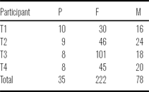
Participant-P was presented target forms in Pinyin, while M and F were presented with target forms written in Chinese characters. Each participant was instructed to repeat the target item three times, but due to the continual need for readjustment of the observation instruments, not all repetitions could be used in the analysis. Table 1 provides a count of the number of viable tokens collected for each participant.
Number of tokens by tone and context.

2.2 Simultaneous laryngeal ultrasound and laryngoscopy (SLLUS)
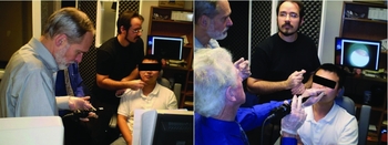
For the SLLUS methodology, a standard laryngoscopic examination was performed. The physician in charge was seated in front of the participant while the laryngeal ultrasound examination was performed simultaneously by approaching the subject from the side. This is illustrated in Figure 1.
Two images showing the setup for the simultaneous laryngoscopy and laryngeal ultrasound. The image on the left shows the laryngeal ultrasound being administered while the laryngoscope is prepared for insertion. The image on the right shows the laryngoscopy being performed by the physician while the laryngeal ultrasound is momentarily being suspended.

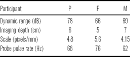
The ultrasound machine used was a portable LOGIQe R5.0.1 system (2004, General Electric Corporation) with an 8C-RS probe (also developed by General Electric). The probe pulse frequency was 10 MHz, which was found through experimentation to allow for suitably clear resolution of the laryngeal structures. The field of view was consistently set to 120°. It was necessary to use speaker specific settings for imaging depth (see Table 2). A Sennheiser ME66-K6 shotgun microphone was used during the examination to record the audio signal, which was digitized at 44100 Hz (16 bit), using an M-Audio Mobile Pre-Amp as an external sound card. The video of the ultrasound machine was captured using an XtremeRGB video card at 30 frames per secondFootnote 3 (uncompressed, 8-bit grey scale, 1024 × 768 pixels), and both signals were captured using Sony Vegas Pro (version 8.0b).
Ultrasound depth settings for each participant.

The laryngoscopy equipment used in this study is an Olympus ENF-P3 flexible fiberoptic nasal laryngoscope fitted with a 28 mm wide-angle lens to a Panasonic KS152 camera. The video signal was recorded using a Sony DCR-T4V17 digital camcorder. The camcorder also recorded an additional audio signal to aid in synchronization of the laryngoscopy data with the laryngeal ultrasound. The laryngoscopy data were then captured to hard disk using Sony Vegas Pro, after which point the two video signals were manually aligned with the aid of the corresponding audio signals.
Coordinating the two instruments was challenging. The major problem was to balance the goals of ensuring participant comfort and a good laryngoscopic view, while at the same time maintaining consistent position and orientation of the ultrasound probe. Although during the performance of individual tokens, the setup remained reasonably stationary, it was necessary to readjust several times during a session (which lasted around 15–30 minutes). Thus, it was most convenient to the examiner and beneficial to the participant to use manual ultrasound probe placement and stabilization: a fixed probe apparatus would require greater effort and time to readjust and fixing the participant's head in place is not ideal when performing laryngoscopy, for safety reasons. Thus, we decided that the benefits of manual probe placement outweighed the costs. This means that throughout the session minor changes in probe position and orientation inevitably occurred, just as they occurred to the position and orientation of the laryngoscope.
We believe that the confounding factors of inconstant probe position and orientation do not impact our results significantly for three reasons. Firstly, on a short time scale, i.e. a token-by-token basis, change in probe position and orientation relative to change in laryngeal position should be minor if not entirely negligible. Secondly, our measurement technique for larynx height, optical flow, does not require tracking a specific object; rather, it relies on global motion, and thus, while the exact view of the larynx may be different for any two randomly selected tokens from a participant's data, what really matters is whether the probe was stationary within a given token, which we believe is the case for all the data we used in the analysis. Finally, every token was independently inspected during the segmentation process (see below); tokens showing bad probe contact (loss of image) or obvious changes in probe position were discarded.
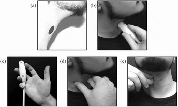
In an effort to achieve the best probe stability possible, we took the following measures. During each examination, the participant was seated in an examination chair equipped with a head rest to help provide stabilization. The ultrasound probe was applied manually to the participant's right thyroid lamina near the laryngeal prominence (Figure 2a and b). The probe was held such that the examiner's thumb was free (Figure 2c) to anchor on the side of the participant's neck, while the index finger was rested lightly on top of the probe (on the orientation notch) for orientation stability and to press lightly against the participant's upper neck (below the chin) to help minimize probe migration (Figure 2d and e). Before elicitation commenced, the participant was instructed to produce an [i] vowel at a normal pitch so that the vocal folds could be located and centered in the ultrasound view. Occasionally, when probe readjustment was required (due to changing the laryngoscope configuration), the participant was instructed to swallow and to produce glides into high and low pitches to ensure that there was still a reasonable registration of changes in larynx height.
Illustration of ultrasound probe placement. In (a), the gray elliptical region shows the approximate probe target area on the neck; (b) is a side view illustrating probe positioning on the neck (with the hand kept clear for visibility of probe location); (c) illustrates how the probe was held; (d) shows a side view of thumb anchoring and index finger contact on the neck; (e) illustrates probe positioning from the front.

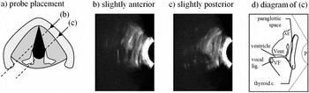
Due to the curvature of the neck, it is very difficult to obtain a perfectly coronal section of the larynx using laryngeal ultrasound (substantial force would be required and this would undoubtedly lead to discomfort for the participant). Gentle positioning of the probe results in a semi-coronal/oblique imaging plane: Figure 3 provides an illustration of the appearance of the larynx in laryngeal ultrasound images obtained from such an imaging plane. In the video from which images (b) and (c) were obtained, the vocal folds are vibrating to produce modal phonation and their movement can be seen as a continual flickering in the brightness pattern. In static images of laryngeal ultrasound, it is much more difficult to locate the vocal folds due to their poor echo-density. The diagram in (d) attempts to delineate the vocal fold on the basis of its appearance in the video.
Illustration of what was observed in coronal laryngeal ultrasound. Schematic (a) shows position of transducer probe relative to thyroid cartilage in the axial plane and is cross-referenced with images (b), (c), and (e). Image (b) is laryngeal ultrasound (top of image is superior) with a slightly anterior probe placement, and (c) has slightly posterior probe placement. Diagram (d) corresponds with the ultrasound image in (c). VF = vocal fold; Vent = ventricular fold; AE = aryepiglottic fold; P = probe location.

Once all data were captured and aligned in Sony Vegas Pro, each token was manually segmented into a pair of files: one for the laryngeal ultrasound and one for the laryngoscopy, each with its own audio track. During the segmentation process, care was taken to ensure that alignment was maintained among all of the signals. The two audio signals could be compared at the sample level for precision of global alignment between the laryngoscopy and the laryngeal ultrasound. Alignment between the audio and video of each of these data sources was confirmed through manual inspection.
2.3 Data analysis
Temporal regions of interest (ROIs) were defined over the voiced part of the syllable being analyzed, and the STRAIGHT algorithm (Kawahara, de Cheveigné & Patterson Reference Kawahara, de Cheveigné and Patterson1998) was used to obtain f0 traces of this region. Larynx state was assessed using laryngoscopic video frames within the ROI. The primary objective of this analysis is to identify the activity of the laryngeal constrictor mechanism (Esling & Harris Reference Esling, Harris, William and Beck2005, Edmondson & Esling Reference Edmondson and Esling2006). The approach taken was to categorize the images of the larynx using two criteria: whether the larynx appeared constricted (C) or not (U) and whether the larynx appeared to be raised (R), at neutral height (N), or lowered (L). Additionally, a (+) and a (−) were used to add further specificity to the observed change in larynx height. Observing changes in larynx height from the laryngoscopic video allowed us to corroborate observations of change in larynx height obtained from the laryngeal ultrasound video.
The concept of laryngeal constriction is particularly important in this study, and thus it is worthwhile to outline briefly what it entails. The view we take here stems from anatomical (e.g. Negus Reference Negus1949; Fink Reference Fink1974, Reference Fink1975), singing (e.g. Estill & Colton Reference Estill and Colton1979, Yanagisawa et al. Reference Yanagisawa, Estill, Kmucha and Leder1989), and phonetic (e.g. Lindqvist-Gauffin Reference Lindqvist-Gauffin1969, Reference Lindqvist-Gauffin1972; Iwata et al. Reference Iwata, Sawashima, Hirose and Niimi1979; Traill Reference Traill, Singer and Lundy1986; Painter Reference Painter1986, Reference Painter1991; Edmondson & Esling Reference Edmondson and Esling2006; Esling Reference Esling1996, Reference Esling1999, Reference Esling2005) research. Laryngeal constriction, as defined by Esling (Reference Esling2005), involves the narrowing of the laryngeal airway of the epilaryngeal tube (ventricle and vestibule) through the synergistic participation of three mechanisms: (i) contraction of the intrinsic, constricting laryngeal musculature: the external thyroarytenoids, the thyroepiglotticus, and the muscle chain formed by the lateral crico-arytenoids, oblique interarytenoids, and the aryepiglottic muscles (Lindqvist-Gauffin Reference Lindqvist-Gauffin1972; Fink Reference Fink1974, Reference Fink1975; Esling et al. Reference Esling, Zeroual and Crevier-Buchman2007); (ii) larynx raising, driven by the thyrohyoid muscles, the suprahyoid muscles of the jaw and tongue, and the pharyngeal musculature (palatopharyngeus, stylopharyngeus, salpingopharyngeus, and the inferior and medial pharyngeal constrictors; see e.g. Shin et al. Reference Shin, Hirano, Maeyama, Nozoe, Ohkubo, Stevens and Hirano1981, Zemlin Reference Zemlin1998); and (iii), retraction of the tongue and, concomitantly, the epiglottis. These three factors all conspire to cause folding, buckling, and compaction of the soft tissues within the larynx. With sufficient constriction it is possible to cause apposition of the cuneiform tubercles and aryepiglottic folds to the lower body of the epiglottis in the region of the epiglottic tubercle. With adducted vocal folds, the laryngeal constriction mechanism can cause vocal-ventricular contact to occur, a gesture we refer to as ventricular incursion (following Edmondson & Esling Reference Edmondson and Esling2006), which is predicted to hinder normal vocal fold dynamics (see e.g. Laver Reference Laver1980). It is normal to see moderate levels of posteroanterior narrowing of the epilarynx occurring with ventricular incursion, suggesting that the lateral thyroarytenoid muscles play an important role in achieving this configuration.
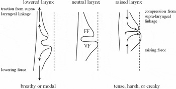
Larynx height is critical in regulating the vertical dimension of laryngeal constriction: raising pushes all of the structures upwards and, if the tongue is not evacuated from the lower pharynx, collision of the tissues within the larynx is inevitable; lowering the larynx causes stretching of the soft tissues, which, on account of their biomechanical properties (e.g. positive Poisson ratio), leads to a thinning and lateralization of the folds, i.e. vocal, ventricular, and aryepiglottic (Fink Reference Fink1974, Reference Fink1975). Thus, laryngeal constriction favours a raised larynx setting (a similar conclusion is reached by Esling Reference Esling1999). Larynx raising, however, does not automatically guarantee that laryngeal constriction will occur: it depends on the engagement level of the other factors. For example, when the posteroanterior axis of constriction is opposed by contraction of the cricothyroid muscles, or when the tongue root is advanced. This is why we can produce high pitch targets with raised larynx and in falsetto mode with no trace of laryngeal constriction. The same is true with larynx lowering; it is still possible to engage moderate levels of constriction (see Esling & Moisik Reference Esling, Moisik, Gibbon, Hirst and Campbell2012) if the other components are sufficiently engaged.
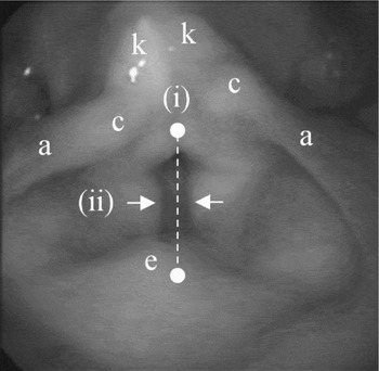
Indicators of laryngeal constriction are as follows: (i) posteroanterior dimension of the epilaryngeal tube, (ii) ventricular incursion (adduction of the ventricular folds and their presumed contact with the vocal folds), (iii) and the elevation of the larynx (Figure 4; see Esling Reference Esling1996, Esling & Harris Reference Esling, Harris, William and Beck2005, Edmondson & Esling Reference Edmondson and Esling2006). In laryngoscopy, changes to larynx height appear as a change in scale of the laryngeal structures; if the larynx rises, it generally appears larger and vice versa for larynx lowering (see Kagaya Reference Kagaya1974). Figure 4 demonstrates indices (i) and (ii) and shows important landmarks of the larynx.
Indicators of laryngeal constriction. (i) Posteroanterior epilaryngeal tube dimension: dashed white line; (ii) ventricular incursion: white arrows. Larynx height (iii) appears as changes in scale and brightness of the laryngeal structures. Structures: aryepiglottic folds (a), cuneiform tubercles (c), epiglottic tubercle (e), and corniculate tubercles (k).

2.3.1 Optical flow analysis of laryngeal ultrasound video
Unlike the laryngoscopy data, the laryngeal ultrasound data are well adapted and amenable to quantitative evaluation for change in larynx height; we accomplish this by means of optical flow analysis. Ultrasound video is generally noisy (Stone Reference Stone2005): subtle variations in tissue position over time can yield different ultrasound echo gradients that appear as random fluctuations of pixel intensity. The best ultrasound imaging occurs for structures that are perpendicular to the ultrasound beam: the structures of the larynx are complex and exhibit many changes in direction, which means that conditions are not always optimal for generating a clear ultrasound image. Furthermore, the larynx includes many regions of adipose tissue, air cavities (such as the ventricle and paraglottic and pre-epiglottic spaces), and various other tissue interfaces (see Hirano & Sato Reference Hirano and Sato1993) which generally have the effect of reducing image clarity and consistency.
Unlike lingual ultrasound research (e.g. Davidson Reference Davidson2006), which typically employs an edge-analysis methodology, laryngeal ultrasound cannot be easily analyzed using a method that tracks a specific structure moving over time. This is because the various structures of the larynx are continually moving into and out of the ultrasound beam's imaging plane during speech. A different approach is to track movement en masse using a technique called optical flow analysis (see Horn & Schunck Reference Horn and Schunck1981). Optical flow is an image analysis technique that allows movement recorded in a sequence of video frames to be quantified as a discrete vector (or velocity) field. The applications for optical flow analysis are numerous and include computer vision for robotics, medical imaging, video surveillance, video compression, and so forth (e.g. Horn & Schunck Reference Horn and Schunck1981, Danilouchkine, Mastik & van der Steen Reference Danilouchkine, Mastik and van der Steen2009). With simple statistical evaluation, optical flow can be used to quantify changes in position of objects in a video, although more sophisticated algorithms can be employed to automatically segment and track moving objects (e.g. Mémin & Pérez Reference Mémin and Pérez1998).
Automation is one of the key benefits of an optical flow analysis. Although automated algorithms exist for edge-detection in lingual ultrasound videos (e.g. EdgeTrak: Li, Kambhamettu & Stone Reference Li, Kambhamettu and Stone2005), these often require manual monitoring to be fully successful (e.g. McCormick, Frisch & Wodzinski Reference McCormick, Frisch and Wodzinski2008), which makes them only semi-automated. There are three primary advantages to conducting an automated analysis of ultrasound video data: (i) it is less time consuming than manual analysis, (ii) it eliminates human error from analysis, and (iii) it is an impartial way to conduct an analysis, avoiding results being skewed by an investigator's personal bias.
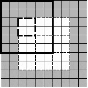
The optical flow algorithm employed hereFootnote 4 is a block-wise, cross-correlation-based method developed for this study using Matlab (version R2009a). Each pair of contiguous frames is decomposed into a grid of equal sized pixel blocks. The algorithm allows the size of these blocks to be specified by the user. There is no optimization procedure for determining the best block size; however, through experimentation, we found that a size of 15 × 15 pixels generally provides a good trade-off between analysis resolution and robust results. Each block is augmented during analysis to three times its original size; pixel data surrounding the analysis block on all sides are included in the analysis, meaning that the analysis blocks overlap each other. The purpose of this is to eliminate the influence of noise in the image: the larger the analysis area, the less the chance that noisy variations in an image will confound the analysis. To improve the accuracy of the analysis, an adjustment is made to the analysis block images so that fine-grained noise is eliminated: every analysis block is dilated using a 3-by-3 square morphological structuring element.Footnote 5 Analysis blocks on the edge of the image were zero padded in block regions where there is no image. Figure 5 presents an illustration of how the block-wise analysis divides up an image.
A hypothetical illustration of how images are decomposed into sets of blocks in the optical flow analysis. White squares represent pixels of an image; gray squares represent zero padding. Light dashed lines delineate 2-by-2 analysis blocks. The bold line shows an example of an augmented block around its corresponding analysis block (bold dashed line) that is on the edge of the image and thus includes the zero-padded region as well.

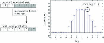
Illustration of how the cross-correlation analysis detects movement between pairs of frames. On the left are a pair of example pixel strips; on the right is a stem plot showing the results of the cross-correlation analysis. In this case, positive lag values indicate movement to the right.

The cross-correlation part of the analysis has two phases: a horizontal phase and a vertical one. These analysis phases eventually become the corresponding horizontal and vertical components of the optical flow vector for the analysis block. In either phase (horizontal or vertical), the analysis blocks from the current and next frames are decomposed into corresponding strips of pixels: rows for the horizontal phase and columns for the vertical phase. Each set of current and next pixel strips is then subjected to cross-correlation analysis, which allows the difference between the current and next frames to be quantified by determining which of the cross-correlation lags furthest from the zero-lag has the largest correlation.Footnote 6 This is illustrated in Figure 6 for a hypothetical horizontal component. On the left side of the figure are two pixel strips that have been extracted from a hypothetical analysis block, the top one from the first frame in a sequence, or ‘current frame’, and the bottom from the second, or ‘next frame’ (white pixels represent part of an object in the image). Cross-correlation analysis of their pixel values provides an estimation of the difference between the two frames in terms of cross-correlation lag units, which in this case represent pixels. The highest lag number (in terms of absolute value) associated with the highest correlation is lag +4, which indicates movement to the right by four pixels: this is in fact precisely what has occurred in the pixel strips.
In the simple case, the value of the lag with the highest correlation value is distinct from subsequent lags in terms of correlation value; however, occasionally the cross-correlation sequence is not monotonic up to the correlation peak (e.g. in the case of periodic correlation) or does not have a distinct cut-off point, making estimation of the difference between the frames difficult. Thus, the maximum lag is defined as the lag that has the highest absolute lag value of the top ten percent of all lag correlations. Once the cross-correlation has been performed across the set of pixel strips, the averages of the maximum lag values for each component are taken as components for the output optical flow vector for the analysis block. The entire optical flow field is constructed by running this analysis for all analysis blocks that make up the entire image.
Once the optical flow field has been generated, movement is determined by averaging the top 25% of vectors (based on magnitude). This was done to reduce average skewing due to null vectors (where no movement occurred or the image was blank in one of the frames) or vectors with very small magnitudes (usually generated in very noisy regions). Velocity along a particular dimension is determined simply by obtaining the value for the corresponding componentFootnote 7 in the averaged flow vector across time (from one frame pair to the next). The velocity data can then be numerically integrated with a cumulative trapezoidal numerical integratorFootnote 8 to obtain an estimate of the evolution of movement along a particular dimension over time. Since no constant of integration can be supplied to the algorithm (because, in the case of the present study, absolute laryngeal height is unknown), the integrator always starts at zero displacement. Finally, since the optical flow algorithm measures movement primarily in units of pixels, the output of the algorithm is scaled into units of millimetres (the scaling ratios for each participant's data are included in Table 2). This scaling is possible because the ultrasound machine superimposes a ruler on the side of the ultrasound image it creates, allowing for quantification of movement in familiar units of distance.
2.3.2 Test case for validating the optical flow algorithm
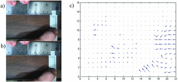
In order to ensure the accuracy of the optical flow algorithm employed in this study, a test case was developed that permitted the velocity of a moving object and the distance it travels to be assessed with certainty. The test case is a video of a flat metal bar being moved along a ruler (see Figure 7a, b). To illustrate how the optical flow analysis works, the first two frames of this video are shown (Figure 7a, b) next to the corresponding optical flow analysis, which is shown as a vector field (Figure 7c). This type of plot shows the patterns of motion that occurred between pairs of frames: for example, note how most of the flow vectors are on the right side of the plot and pointing leftwards: this corresponds to the moving image of the metal bar and thumb in the video frames.
Frames 1 (a) and 2 (b) from the test case video showing a movement of the metal bar approximately 4 mm to the left. The corresponding results from the optical flow analysis of this frame pair are shown in the form of a vector field plot (c).

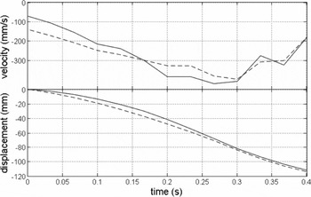
In the test video, the metal bar was determined to move a total distance of approximately 11.0 cm in 0.4 s; the top plot in Figure 8 shows its actual velocity (solid line) along with the velocity estimate (dashed line) produced by the optical flow algorithm. The bottom plot in Figure 8 shows the change in position of the metal bar over time: these position contours are produced by the cumulative trapezoidal numerical integrator.
Plot of the velocity and position of the metal bar in the test case as determined by manual measurement (solid line) and by the optical flow algorithm (dashed line). The negative values indicate movement to the left.

The normalized RMS error of the optical flow estimate of the velocity function is 12.17%; the match with the manual measurement is visually very close (Figure 8). Each velocity contour was numerically integrated as described in the previous section (3.5.1) to determine the total distance travelled by the bar according to the speed plots (see bottom plot in Figure 8): the integral of the actual speed contour was found to be 11.14 cm (111.4 mm) and the integral of the estimated speed contour was found to be 11.35 cm (113.5 mm). The estimated value differs from the actual value by 1.8%.
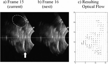
As a final demonstration of the optical flow algorithm, Figure 9 provides a pair of contiguous frames from Participant-P's laryngeal ultrasound video data. These frames show an instance of laryngeal descent (a 2 mm drop): a white dotted line is superimposed over the frames to facilitate comparison between the frames. The view of the larynx seen in the ultrasound shows one half of the laryngeal structures in the coronal plane. A white arrow is used to indicate the location of the bottom of the thyroid lamina and the vocal folds themselves fall roughly below the white dotted line. The structures above the white line are sections of the epiglottis and laryngeal vestibule. A white dashed-ellipse is used to delineate the approximate region of the acoustic shadow cast by the hyoid bone. The ultrasound probe head is represented as a semi-circular area of darkness on the right side of the frame.
A visual demonstration of the optical flow analysis on data from Participant-P. Images (a) and (b) represent a pair of contiguous frames in the laryngeal ultrasound video data showing descent of the larynx; the plot in (c) shows the resulting downward-directed optical flow field. Dotted line: reference line to facilitate comparison; white arrow: the location of the bottom of the thyroid lamina; white dashed ellipse: acoustic shadow cast by the hyoid bone.

The vector field plot in Figure 9c shows the resulting optical flow field generated from the optical flow analysis. The vectors in this flow field largely point downwards indicating that the primary movement in the frame is descent of the larynx. Also note that in this analysis there are 23-by-15 analysis blocks, each of which is associated with its own optical flow vector. Some of these vectors are null and appear as dots rather than arrows (largely in the upper and bottom left corners of the plot where no laryngeal structures were imaged).
2.4 Methodology summary
The research method combines laryngoscopy and laryngeal ultrasound (SLLUS) to study the four tones of Modern Standard Chinese (MSC) in citation form. There are three main aspects to the data that were analyzed. The first is f0 contour extraction from the audio signal, which was done using the STRAIGHT algorithm (Kawahara et al. Reference Kawahara, de Cheveigné and Patterson1998). The laryngoscopy was examined qualitatively to identify laryngeal state during tone production and also to corroborate the quantification of laryngeal height obtained from the laryngeal ultrasound. This larynx-height quantification is at the heart of the study and was based on an optical flow analysis of the laryngeal ultrasound data. The optical flow analysis, which has been validated with independent data, produces velocity fields for the laryngeal ultrasound video data which were assessed for movement in the vertical direction using statistical methods. The output of this process is a set of velocity signals which were integrated over time to obtain the larynx-height data, and this integration always started at zero displacement.
3 Results
The results are broken into three sections: Section 3.1 provides a statistical overview of the data, focusing on broad tendencies across the speakers concerning tone durations and ranges for f0 and larynx height. Section 3.2 presents time-normalized contour data of f0 and larynx height analyzed using linear regression and smoothing spline ANOVA (SS ANOVA; Davidson Reference Davidson2006). Finally, Section 3.3 presents case studies of noteworthy tokens; the focus is on the relationship between the appearance of the larynx in the laryngoscopy and the vertical change in larynx position.
3.1 Descriptive overview: Duration, f0, larynx height, and f0 and larynx height velocities
Overall variation in the data for duration, f0, and larynx height of the citation-form tones is presented in Figure 10. (As a reminder: T1 = high level, T2 = mid rising, T3 = falling rising, and T4 = high falling.)
Plots for duration (top), f0 (middle left), larynx height (middle right), f0 velocity (bottom left; calculated using the forward difference quotient discretely defined by f0 values at sampled intervals), and vertical larynx velocity (bottom right) variation found in the data set for the three participants. P = male phonetician; F = native female; M = native male; N = number of tokens.

The general pattern for tone duration upheld across all three participants is that, unsurprisingly, T4 is the shortest in duration. T3 is the longest for Participant-P and Participant-M, but it is approximately equivalent in duration to T1 for Participant-F. Plots for f0 and larynx height reveal an inverse relationship between the male and female participants: male participants exhibit less extreme f0 excursions over a lower f0 range than the female; conversely, the female exhibits a less extreme larynx height excursion than the males. This difference in f0 between the male and female participants is unsurprising: females generally have higher and wider f0 levels than males. The results for larynx height suggest that the males rely more heavily upon larynx height to execute f0 changes; but without normalizing for speaker size and without a larger sampling of speakers, it is difficult to draw a firm conclusion on this matter. An attempt at normalization is made in Section 4.2. The female also is unique in exhibiting a bias towards raising the larynx, a fact which will become important below.
The f0 and vertical larynx velocity plots at the bottom of Figure 10 show how duration and tonal contour impact the kinematics of tone production. The most important pattern illustrated in these plots is the large negative velocities for T4 in terms of f0 and larynx height, which, given the short duration of T4, is to be expected. Participant-F shows the most negative larynx velocity for T4, which suggests that when she is under greater time pressure to achieve a rapid drop in pitch she employs the larynx-lowering mechanism. This is unlike her method for producing T3, which critically does not involve larynx lowering during the falling part of the tone.
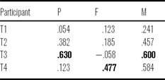
Correlations between the velocity variables by participant and by tone are shown in Table 3. Larynx velocity most strongly correlates with f0 velocity for T3 in the case of Participant-P and M; the correlation is actually slightly negative for Participant-F, which results from the fact that f0 is dropping while the larynx is (slightly) raising. For the native speakers, the correlation between the velocity variables is also considerable for T4, which points to the increased importance of larynx height in the production of this tone, which is the shortest of them all (in citation form).
Vertical larynx velocity and f0 velocity correlation by speaker and tone (the largest correlations are in bold).

3.2 Analytical overview: SS ANOVA and correlation of f0 and larynx height
In this section, time-normalized plots of f0 and larynx height illustrate the overall movement patterns of the larynx in relation to the tonal f0 contours for each of the four Mandarin tones by context. Smoothing Spline ANOVAs (SS ANOVA; see Davidson Reference Davidson2006) were performed to create each of the time-normalized contour plots. The contour lines show the smoothing spline fit for each of the tones, and the gray regions show the 95% confidence intervals (based on the ANOVA component of the SS ANOVA algorithm). Regions where the intervals overlap are not significantly different. Wider confidence intervals are a product of greater variance in the data (particularly for Participant-F's larynx height data). Tones are labelled on each plot and the line style designates specific tones: T1 is the solid line, T2 is the dash-dotted line, T3 is the dashed line and T4 is the dotted line.
In each case, below the contour plots are two scatter plots showing the correlation between change in f0 relative to change in larynx height. The left hand plot combines data for all tones and the right hand plot shows data for only T3, which is done to reveal an asymmetry in the laryngeal height behaviour between the male participants (P and M) and the female (F). Each of these correlations is produced by dividing each token into ten contiguous segments and averaging the sample points within each of these segments. Since each token consists of exactly 100 samples (as a result of the time normalization), there are ten samples per averaged segment used in the correlation. Data greater than three standard deviations above the mean were discarded.
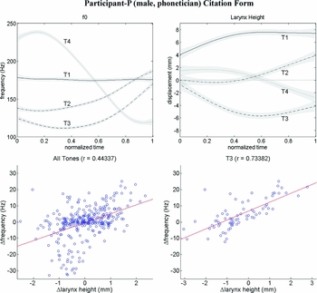
The data for Participant-P (male, phonetician) are illustrated in Figure 11. We take these productions to represent canonical phonetic forms of the four tones: T1 is level, T2 is mid rising, T3 is falling rising, and T4 is falling. When these f0 contours are considered in relation to the larynx-height contours, some notable patterns emerge. First, although T1 is produced with a relatively stable f0, the larynx shows a tendency to gradually rise through the production of the tone; we will show below that this also occurs for the other participants. For T2 and T4, the larynx-height contours generally reflect the corresponding f0 contours. There is, however, a difference in rate of change between the f0 contours of T2 and T4 that is not reflected in the larynx height pattern. Finally, T3 exhibits larynx lowering, which reaches its nadir roughly halfway through the tone where the f0 is also low; the larynx then ascends in correspondence with the rising f0 at this point. There is a moderately strong positive correlation between change in f0 and change in larynx height (r = .44) for all tones, indicating that larynx height movement patterns are partially predicted by the shape of f0 contour. The contour plots clearly indicate that the velocity of f0 change is greater than that observed for larynx height. This reveals that there is obviously another factor at play – most likely the action of the cricothyroid muscle. Isolating T3 in the correlation analysis shows a much stronger correlation between the two variables (r = .74) than when the tones are grouped together: this increased correlation for T3 underscores the relationship between lowering the larynx and achieving a low f0.
Time-normalized plots of f0 and larynx height (top row) and scatter plots showing correlations between these two variables (bottom row) of the tones produced in citation form by Participant-P.

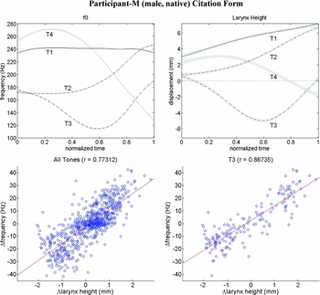
The relationship between f0 and larynx height for Participant-M is illustrated in Figure 12. The f0 contours alone for this participant are characteristic for citation form productions of the tones and are parallel to the canonical forms produced by the phonetician (Participant-P). The relationship between larynx height and f0 for the native speaker is also similar to what we observed for the canonical forms produced by the phonetician. T1 in citation form shows a stable f0 in correspondence with a gradually rising larynx position. T2 and T4 once again show a strong relationship between f0 contour and larynx-height contour, although, again the velocity of change is evidently greater for f0 than for larynx height. Upon visual inspection, the contours for T3 are nearly identical, something which the correlation analysis for this tone confirms, as the two variables are highly correlated (r = .87). Overall, as the correlation analysis shows, change in f0 and change in larynx height are strongly correlated for Participant-M (r = .77), even more so than for Participant-P.
Time-normalized plots of f0 and larynx height (top row) and scatter plots showing correlations between these two variables (bottom row) of the tones produced in citation form by Participant-M (all tones on left, T3 on right).

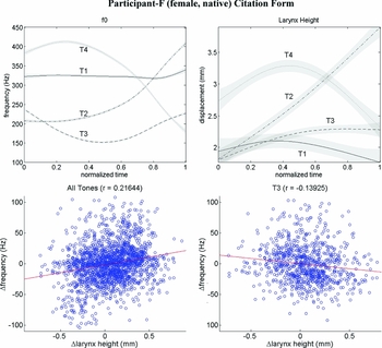
Contour and correlation plots for Participant-F (female, native) are shown in Figure 13. Once again, the expected f0 contour patterns are observed, and thus all three participants agree in this regard. The larynx-height contours for Participant-F have broader confidence intervals than they do for the other participants: this indicates more variance in the data for this participant. Nevertheless, clearly distinguishable larynx-height patterns still emerge from the SS ANOVA. T1 shows an initial rise in larynx height and then a slight descent while f0 is relatively flat. T2 and T4 show larynx-height contours that generally correspond with the f0 movement pattern, but there is some asynchrony. Larynx movement during T2 is nearly linear with a high rate of change; however, the f0 for T2 shows a delayed rise. In T4, larynx height peaks towards the middle of the production despite f0 reaching its peak much earlier; however, f0 and larynx height do descend nearly synchronously and with similar slopes. Also, note that T4 shows the most larynx lowering of any of the tones, although there is no net descent across the tone due to the initial rise.
Time-normalized plots of f0 and larynx height (top row) and scatter plots showing correlations between these two variables (bottom row) of the tones produced in citation form by Participant-F (all tones on left, T3 on right).

The persistently high laryngeal position for T3 is unexpected, particularly since this tone has the lowest f0 of all the tones. This stands in stark contrast to the male participants (P and M), who show the greatest degree of larynx lowering for the low part of T3. The correlation plot for all tones shows that there is generally only a weak positive correlation between change in larynx height and change in f0 (r = .22); importantly, unlike the male participants, Participant-F shows a negative correlation between change in larynx height and change in f0 for T3 (r = −.14).
We have observed the following facts about the nature of larynx height during citation or canonical Mandarin tone production. T1 shows gradual larynx raising. T2 and T4 show a positive relationship between larynx height and f0, but f0 exhibits a higher rate of change than larynx height. T3 shows two patterns with regard to its low f0 part: the male participants use larynx lowering and the female uses larynx raising (we wish to emphasize here that, while these patterns do correspond with speaker gender, and sexual dimorphism of the larynx may in part explain the difference, our focus is on varying phonetic possibilities for laryngeal control). Finally, larynx height generally increases or decreases with f0, as the correlation analysis indicates, but the change is not always perfectly synchronous.
3.2 Careful phonetic production of Mandarin tones
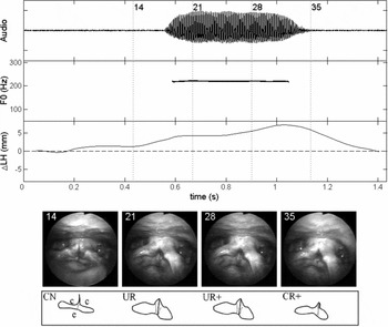
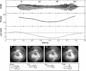
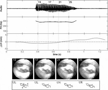
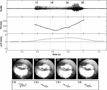
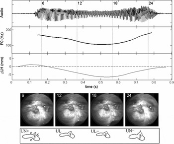
Several case studies of individual tone tokens for each of the participants are presented in this section to illustrate the full methodology of simultaneous laryngoscopy and laryngeal ultrasound (SLLUS) and to support the observations made in the previous two sections (3.1 and 3.2). There are two subsections – one for the phonetician and one for the native speakers. The reason for the selection of the illustrated tones will be made clear in each subsection and, due to space limitations, not all tones are illustrated. In general, the selection is based on the clarity of the laryngoscopy, how well a given token illustrates a participant's canonical production strategy, and how clearly the laryngoscopy corroborates the larynx height data. Each of the case studies shows the acoustic waveform, f0 contour, larynx-height contour (change in larynx height), and four manually selected laryngoscopy frames (the time locations of which are marked on the plots with dashed vertical lines and the corresponding frame number to facilitate identification). No frames are illustrated from the laryngeal ultrasound video data because these are not as useful as the larynx-height contour itself in interpreting the data patterns.
The syllable [ti] was chosen to illustrate productions for Participant-P, [pi] was selected for Participant-F and [ji] was selected to illustrate those of Participant-M. It was not possible to choose one single syllable for all participants because no syllable was found to have optimal laryngoscopic views for all participants. However, the effects of the different syllable types are assumed to be minimal or negligible given that they all share the same vowel and conform to the overall contour patterns outlined above in Section 3.2, which represents a combination of all syllable types.
The time domain of each of these tokens is expanded beyond the voiced part of the tone-bearing syllable; this allows laryngeal movements that occur before and after the actual token to be shown, and it helps to contextualize some of the movements of the larynx that occur during the syllable itself. The data and statistical description (presented in Sections 3.1 and 3.2) are based solely on the voiced part of the token syllable, and the temporal expansion is purely for expository purposes. The laryngoscopy videos are marked with code letters to indicate the qualitative assessment of the state of the larynx according to whether it is constricted or not (constricted = C; unconstricted = U) and the estimated height of the larynx (L = lowered; N = neutral; R = raised); plus ‘+’ and minus ‘−’ mark indicate finer detail in terms of raising and lowering, respectively, relative to other frames.
3.3.1 SLLUS case study for Participant-P
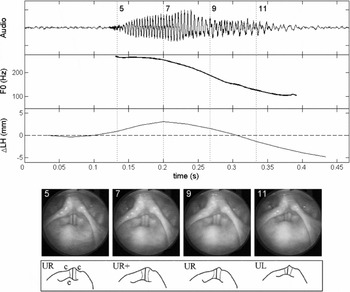
The first case study demonstrates T4 for Participant-P. This tone is presented because it provides a good illustration of how the laryngoscopy corroborates the larynx height data.
In Figure 14, the larynx rises 3 mm from Frame 5 to Frame 7 and then begins a descent of about 5 mm from Frame 7 to Frame 11. Although f0 does not show the initial rise, both variables appear similar in their descent profile. It is possible that initial larynx raising is being used as a complement to CT action to attain the high f0 level, but lags behind f0 movement (and, by implication, CT action) possibly because structures involved are more massive and thus accelerate more slowly than changes made to f0 using the CT muscles.
Case study of Participant-P's T4 in [ti51]. LH = larynx height; Laryngoscopy tracings: epilaryngeal tube outline (solid line); ventricular fold edges (dotted lines); glottis (solid line); c = location of the cuneiform tubercle; e = epiglottic tubercle.

It would be very difficult to quantify the change in larynx height from the laryngoscopy alone, even though the visual impression is evidently that the larynx is in descent from Frames 7 to 11. This visual impression of descent is discerned from several factors (see Kagaya Reference Kagaya1974): the reduced scale of the laryngeal structures, an increase in the amount of visible surface of the epiglottis and aryepiglottic folds, and a decrease in the reflections off of the surface of the laryngeal mucosa (indicating greater distance from the laryngoscope light source). The laryngoscopy also provides evidence that the larynx remains unconstricted in its descent: even though the posteroanterior distance of the epilaryngeal tube narrows slightly because of anterior cricoid rotation (see Section 2.1 above, also Honda et al. Reference Honda, Hirai, Masaki and Shimada1999), the vocal folds are free of ventricular incursion. Furthermore, we infer that vertical separation between the vocal and ventricular folds also occurs in the way described by Fink (Reference Fink1974). Thus, we conclude that there is no laryngeal constriction occurring. In fact, the vocal folds have roughly the same amount of exposed surface area in all of the frames.
3.3.2 SLLUS case studies of native production of Mandarin tones
We now illustrate the SLLUS data of bona fide citation-form productions of Mandarin tones. We have chosen to exhibit T1 and T3 for both participants (M and F). The other tones, T2 and T4, represent the expected cases where the larynx height correlates positively with f0. We take T1 as the control case to illustrate the appearance of the individual's larynx. The surprising results appear for T3 when we compare the productions of the two speakers. While Participant-M exhibits the canonical larynx-lowering pattern to achieve the low f0 target, Participant-F exhibits the opposite laryngeal movement, and the laryngoscopy allows us to identify that the raising is associated with activation of the laryngeal constrictor.
First, we present two case studies for Participant-M. The first case study is of T1 (Figure 15), which again exhibits larynx raising on the order of 4 mm despite static f0. The laryngeal state for this tone is unconstricted. We can confirm this by comparing Frames 21 and 28, which occur during the syllable, with Frames 14 and 35, which occur immediately before and after the syllable, respectively. Manual traces of the laryngeal states have been added for clarity. In Frames 14 and 35, the larynx is more constricted (as indicated by the dotted lines of the ventricular fold edges) than during the voiced part of the syllable in Frames 21 and 28, when the larynx assumes its typical state for modal phonation for this speaker. Note that in the constriction-neutral state seen in Frames 21 and 28 this participant's larynx exhibits a narrow ventricular aperture. However, it is clear that this merely reflects individual anatomy, by comparing these frames with Frames 14 and 15, where ventricular incursion and narrowing of the posteroanterior dimension of the epilaryngeal tube are manifest. The phonetic result is the initiation and termination of the syllable with glottal stops.
Case study of Participant-M's T1 in [ji55]. LH = larynx height; Laryngoscopy tracings: epilaryngeal tube outline (solid line); ventricular fold edges (dotted lines); glottis (solid line); c = location of the cuneiform tubercle; e = epiglottic tubercle.

The next case study for Participant-M looks at T3 (Figure 16), where we observe larynx lowering in conjunction with f0 lowering and an overall strong visual correlation between the f0 and larynx-height contours. Critically, as we look at the ventricular fold edges (indicated by the dotted lines in the traces), we do not observe any form of laryngeal constriction occurring during the low part of the tone visible in Frames 12 and 18 (compare with laryngeal constriction in Figure 15, Frame 14 or 35). The epilaryngeal aperture does not undergo significant reduction in the posteroanterior dimension, and the relationship between the ventricular folds and vocal folds is consistent from one frame to the next. The laryngoscopy thus provides us with corroborating support for what is observed in the larynx-height change data, and laryngeal constrictor state can be considered continuously unconstricted for this example.
Case study of Participant-M's T3 in [ji213]. LH = larynx height. Laryngoscopy tracings: epilaryngeal tube outline (solid line); ventricular fold edges (dotted lines); glottis (solid line); c = location of the cuneiform tubercle; e = epiglottic tubercle.
The situation is different for Participant-F, who employs a larynx-raising strategy for low f0 production during T3 (see Section 2.3 for a discussion of how larynx raising is complementary to laryngeal constriction). First we demonstrate in Figure 17 the appearance of this participant's unconstricted laryngeal state using T1 as an example. The larynx-height contour indicates that the larynx rises slightly by about 2 mm during the production of T1, but we do not observe much change in laryngeal state in the laryngoscopy. Again, the posteroanterior dimension of the larynx is held fixed throughout, and the vocal folds are not obstructed by the ventricular folds.
Case study of Participant-F's T1 in [pi55]. LH = larynx height; Laryngoscopy tracings: epilaryngeal tube outline (solid line); ventricular fold edges (dotted lines); glottis (solid line); c = location of the cuneiform tubercle; e = epiglottic tubercle.

By comparison, the appearance of the larynx during T3 production undergoes a visible change as seen in Figure 18: it increases in its degree of constriction during the low f0 region of the tone, which is illustrated by Frames 18 and 24. The constriction is evident, once again, in the reduction of the posteroanterior distance of the epilaryngeal tube and ventricular incursion, although the latter is somewhat difficult to see since the right cuneiform tubercle is obstructing these structures. In fact, the observation that the cuneiform tubercle is in contact with the tubercle of the epiglottis provides an argument that the constriction is particularly strong in this example. Another indicator is the position of the epiglottic tubercle, which retracts in Frames 18 and 24. It is also important to point out that the auditory quality of phonation becomes increasingly tense and ultimately creaky during the low part of T3 in general. Creakiness is evident in the audio waveform in Figure 18 particularly between 0.6 and 0.8 s and was observed to be a pervasive feature of this part of the tone for this speaker.
Frames 12 and 30 illustrate the appearance of the larynx during the peripheral parts of this tone where f0 is relatively high: here we do not observe laryngeal constriction of the same extent as in Frames 18 and 24. It is likely that larynx height is acting in two ways in this example. The larynx is raised during the entire tone, and thus can be interpreted as facilitating high tone production, which we have observed in general. The low part of the tone, however, engages a new mode of phonation which is complementary to low f0 production: creakiness. Since creakiness can be a result of laryngeal constriction (Esling & Harris Reference Esling, Harris, William and Beck2005), and laryngeal constriction is complemented by larynx raising, as discussed in Section 2.3, it stands to reason that the larynx raising is also acting to facilitate or help induce the laryngeal constriction and thus a creaky low f0 of the low tone target.
Case study of Participant-F's T3 in [pi213]. LH = larynx height; Laryngoscopy tracings: epilaryngeal tube outline (solid line); ventricular fold edges (dotted lines); glottis (solid line); c = location of the cuneiform tubercle; e = epiglottic tubercle.

4 Discussion: Laryngeal strategies for tone production
This section provides discussion of the two key observations emerging from the results. First, in Section 4.1, we provide a qualitative assessment of speaker idiosyncrasies and how this influences our interpretation of the data. Section 4.2 interprets the general role of larynx height in achieving the citation-form tone targets in Mandarin, which pertains to the differing laryngeal behaviour by gender of our participants and the fact that T1 was consistently produced with larynx raising for all speakers. In Section 4.3, we will address the observation that there are two strategies for the production of low f0 tone targets, which was particularly striking for T3, for which two of our participants used larynx lowering and the other used larynx raising in conjunction with laryngeal constriction.
4.1 Idiosyncratic laryngeal behaviour and voice quality in the data
One salient idiosyncrasy reflected in our data is Participant-F's inherently tense voice quality, which is probably not a function of language since it is present in her speech regardless of what language she is speaking. Her inherent voice quality also tends to involve creakiness, and we take this particular fact to be a matter of idiosyncratic speaker variation and not a function of her gender. That is to say, as far as we know, both males and females are equally likely to use creakiness as part of producing Mandarin tones: creakiness is a possible means for either gender to realize low tones in the language. It is purely incidental that in our sampling of speakers, the female happens to use creakiness more than the males do. What is intriguing about this idiosyncrasy, however, is that despite Participant-F's generally high baseline level of laryngeal tension, it is manifest that there is engagement of additional laryngeal constriction for her Mandarin T3s. We have attempted to illustrate this using Figure 17 and Figure 18. Whether her preference for constriction as a strategy for low tone production (see Section 4.3) is caused by her inherently tense voice quality, one can only speculate, but there is certainly nothing stopping inherently non-creaky individuals from using creakiness in the same way. In fact, Participant-M, whose inherent voice quality tends towards modal, sometimes even breathy quality, did indeed use creakiness in his productions on occasion, particularly in non-citation context (although those data are not included in this study).
4.2 Overcoming vocal fold inertia and subglottal pressure decline
With the considerations outlined in Section 4.1, we can now proceed to make a statement about our interpretation of one of the most basic relationships that can be observed in the data: the difference in laryngeal behaviour between the male participants (P and M) and the female participant (F). The males exhibited broad larynx-height ranges (~20 mm) despite having narrow f0 ranges (~200 Hz); the female participant exhibited almost entirely the opposite pattern: narrow larynx-height range (~5 mm) and broad f0 range (~400 Hz). Assuming a sexual dimorphism scaling factor of 1.6 (Titze Reference Titze1989b) between males and females based on measurements of the membranous portion of the vocal folds, then the expected f0 range for the female, based on the male range, would be 320 Hz. The difference between the expected range (320 Hz) and the observed range (400 Hz) may be accounted for by Participant-F's use of creaky phonation to achieve an extra low f0 and thus expanding her f0 range overall. The low tonal regions produced by the males tended to exhibit some slight breathiness but were otherwise modal. We might predict that males using a ‘creaky T3’ would tend towards a production similar to what was observed for Participant-F, laryngeal constriction and some larynx raising (although it is possible to produce creakiness with lowered larynx, but laryngeal constriction still applies; see Esling & Moisik Reference Esling, Moisik, Gibbon, Hirst and Campbell2012).
The concept of laryngeal inertia (or perhaps vocal fold inertia; see Xu Reference Xu2002: 6; Xu & Sun Reference Xu and Sun2002: 1405), has currency for the present discussion. Xu & Sun (Reference Xu2002) observed that one of the most important gender differences for f0 is the rate of oscillation acceleration of the vocal folds; females were reported to consistently require less time to initiate and halt a change in f0 than males, which is interpreted as indicative of the fact that female vocal folds are less inertive (i.e. less massive) than male vocal folds, and thus they can more rapidly accelerate and decelerate than male vocal folds. The relationship to gender is obviously not a necessary one, as it is the case that some males will have less massive vocal folds and some females will have more massive ones on account of individual variation in size and tissue properties (although gender is likely a reliable predictor of vocal fold inertia).
The results for larynx height in conjunction with the concept of laryngeal inertia indicate an interesting possibility: individuals with greater vocal fold inertia manipulate larynx height as a compensatory mechanism to increase the acceleration and deceleration of the oscillation of the vocal folds. In general, the difference between the participants in terms of syllable duration was minimal (see Figure 10): if anything, Participant-M took slightly longer on average (~100 ms) for T2, T3, and T4 than Participant-F did. This means Participant-M had more time to execute the change, and therefore we might expect that he would show less use of larynx raising. We know, however, that the pattern is just the opposite. In any case, if we assume that all of the participants are generally under the same time pressure to achieve a given change in f0, it stands to reason that, the more massive a person's vocal folds, the more likely they may be to employ larynx height to change f0.
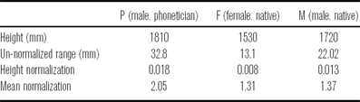
Of course, this relationship remains speculative at this point, because it is not certain whether the measured differences in larynx-height ranges truly reflect greater use of larynx height by the male participants. The other possibility is that the difference is due solely to the size of the participants: a larger person will exhibit larger displacements for any part of their body, not just the larynx. To be more confident with the conclusion that males are using a greater degree of larynx-height manipulation, it is necessary to normalize the larynx-height ranges by participant size; however, the best way to go about doing this is uncertain. The optimal approach would be to normalize by the length of the participant's vocal folds, which ought to strongly correlate with f0. Since we were not able to obtain these measurements, we have attempted two different normalisations to estimate the actual differences in larynx-height range. After removing outliers (greater than one s.d. above the mean), ranges were normalized by participant height, simply by dividing the larynx-height range by the participant's height. Ranges were also normalized by mean membranous vocal fold length (16 mm for males and 10 mm for females; Titze Reference Titze1989b). The results of these normalizations are displayed in Table 4.
A comparison of larynx-height ranges for each speaker using normalization ratios. Mean normalization based on average vocal fold length for males (16 mm) and females (10 mm) as reported by Titze (Reference Titze1989b).

If the variations in larynx height were solely an effect of physical size of the participant, then the normalized values should all be the same. The results of height normalization (see Table 4, Height Normalization row) provide us with an argument that this is not the case: on average, the male participants’ larynx-height range is 37% greater than that of the female participant. The ratios developed using the averages quoted in Titze (Reference Titze1989b) provide a less convincing case: Participant-P exhibits 56% more larynx-height range than Participant-F, but Participant-M only exhibits 4% more range. We take the ratios based on participant height to be more reflective of the actual difference in larynx-height ranges because this index is based on an actual measurement (the participant's actual height), rather than universal mean vocal fold length, where there is uncertainty on how accurate the values are for our participants (given that we could not obtain a measurement of the length of the membranous part of their vocal folds). Admittedly, normalization by height does not guarantee that the differences in range are true either: individuals can have the same height yet vary in other ways (head size, limb size, etc.). Nevertheless, the height normalization is still regarded as the best way available to obtain some degree of confidence that the ranges are in fact different for our male and female participants, with males exhibiting more use of larynx height.
Another argument that larynx height facilitates f0 change can be formed from Participant-F's exceptional use of larynx lowering during T4. This tone is produced under increased time pressure relative to the other tones and has one of the largest f0 ranges of all the tones. We interpret the occurrence of larynx lowering during T4 for Participant-F and the other participants as a sign that deceleration of vocal fold oscillation cannot meet these phonetic criteria by relying upon the relaxation of the cricothyroid muscles alone. Lowering the larynx will increase the rate of deceleration by reducing the tension on the vocal folds by virtue of the cricoid rotation effect described in Honda et al. (Reference Honda, Hirai, Masaki and Shimada1999). The fact that this effect occurs without internal activity of the laryngeal muscles is important, since such activity would likely counter-act the reduction in tension that is required to produce the rapid deceleration of the oscillation of the vocal folds.
Another trend observed in the data that supports the view that larynx height facilitates tone production was the tendency for T1 to be produced with gradual larynx raising (see Figures 11–13). The interesting point is that this generally occurs without a corresponding change in f0. A similar observation is reported by Collier (Reference Collier1975: 250), who notes that cricothyroid contraction increases to compensate for declining subglottal pressure (over a one-second time window); Brunelle, Nguyễn & Nguyễn (Reference Brunelle, Duong Nguyễn and Nguyễn2010: 162) also report the same effect for the A1 (high level) tone in Northern Vietnamese based on inferences of larynx height from laryngoscopic video. We offer the interpretation that the use of larynx raising in this context acts as a compensatory mechanism to mitigate the effect of f0 decline caused by a declining subglottal pressure (see Titze Reference Titze1989a). Under this hypothesis, it is predicted that the effect will be more conspicuous in syllables of longer duration uttered in isolation (as in the citation context). Ultimately it needs to be confirmed that subglottal pressure is indeed dropping at the expected rate such that f0 remains constant under increased larynx raising and the associated increase in vocal fold tension. It is also somewhat surprising that larynx raising occurs when one might expect that increased cricothyroid muscle activity would be sufficient, and it should be entirely possible for the cricothyroid muscles to contract without an increase in larynx height (e.g. Vilkman et al. Reference Vilkman, Sonninen, Hurme and Körkkö1996). The answer may lie in the fact that for T1 the cricothyroid muscles are strongly activated in the first place (Sagart et al. Reference Sagart, Hallé, de Boysson-Bardies and Arabia-Guidet1986, Hallé Reference Hallé1994) to achieve the high f0 target. Further contraction may be more taxing on the system than engaging the larynx-raising mechanism or it might even overcompensate for f0 decline and result in a non-level f0 contour. The fact that larynx raising occurs with f0 raising in general supports this observation, since if CT action were fully sufficient for f0 regulation, we would not observe a change in larynx height at all. The observations then support the view that larynx-height manipulation is a basic component of f0 control and serves to complement intrinsic factors.
4.3 Two strategies for low tone target production
In the basic model of f0 regulation (e.g. Hirose, Simada & Fujimura Reference Hirose, Simada and Fujimura1970; Ohala & Hirose Reference Ohala and Hirose1970; Honda Reference Honda, Bell-Berti and Raphael1995, Reference Honda2004; Zemlin Reference Zemlin1998), the cricothyroid muscles (CT) play an important role in changing the longitudinal tension of the vocal folds – the main factor in determining their fundamental rate of oscillation. But other factors can be significant, for instance, thyroarytenoid activity (Titze, Luschei & Hirano Reference Titze, Luschei and Hirano1989, Honda Reference Honda, Bell-Berti and Raphael1995), subglottal pressure (Titze Reference Titze1989a), or – most important for the present discussion – the height of the larynx. Laryngeal raising mechanisms such as the hyomandibular muscle group (mainly the geniohyoid and anterior digastric muscles), genioglossus (Whalen et al. Reference Whalen1998) and thyrohyoid muscles can induce tension on the vocal folds by translation or rotation of the thyroid cartilage that favours their elongation (Honda Reference Honda, Bell-Berti and Raphael1995, Vilkman et al. Reference Vilkman, Sonninen, Hurme and Körkkö1996), thus raising f0. Larynx lowering, which is driven by the infrahyoid strap muscles (sternothyroid and sternohyoid muscles), typically has the opposite effect: it reduces vocal fold tension, thus lowering f0 (Faaborg-Anderson & Sonninen Reference Faaborg-Anderson and Sonninen1960, Ohala & Hirose Reference Ohala and Hirose1970, Simada & Hirose Reference Simada and Hirose1970, Ohala Reference Ohala1972). On the basis of MRI data, Honda et al. (Reference Honda, Hirai, Masaki and Shimada1999) provide the insight that lowering the larynx causes cricoid rotation favouring vocal fold shortening as the structure moves along the anterior curvature of the cervical spine. Importantly, the body of the vocal folds, i.e. the thyroarytenoid muscles, do not need to contract for this shortening to occur, unlike the situation that occurs for pure isotonic contraction of the thyroarytenoid muscles to lower f0 (Honda Reference Honda, Bell-Berti and Raphael1995: 221). In the case of Mandarin specifically, Sagart et al. (Reference Sagart, Hallé, de Boysson-Bardies and Arabia-Guidet1986) and Hallé (Reference Hallé1994) have both attested, using EMG, that there is infrahyoid strap muscle activity for mid-low tone targets, supporting the claim that larynx lowering plays a role in low tone production. Erickson (Reference Erickson1993) reports similar results for Thai.
We have established that larynx height should correlate positively with f0, which is what we have observed in the general case in our own data. But we also observed that, in addition to larynx lowering for the low f0 target of T3, it is possible to raise the larynx and achieve the same effect of low f0. This seemingly counterintuitive strategy finds its explanation in what can be observed in the laryngoscopy data for Participant-F: the larynx constricts. The acoustic product is usually creaky phonation, which indicates that the vocal folds are undergoing a change in mode of vibration during this adjustment. Creaky phonation has been previously observed to occur generally in Mandarin during low f0 regions of the tones, particularly in citation or terminal form (Davison Reference Davison1991; Belotel-Grenié & Grenié Reference Belotel-Grenié and Grenié1994, Reference Belotel-Grenié and Grenié1995, Reference Belotel-Grenié and Grenié2004; Keating & Esposito Reference Keating and Esposito2006: 89).
To explain the relationship between laryngeal constriction and creaky phonation, we posit that one of the effects of laryngeal constriction is to bring the ventricular folds into contact with the vocal folds, which Edmondson & Esling (Reference Edmondson and Esling2006: 159) refer to as ventricular incursion (also see Lindqvist-Gauffin Reference Lindqvist-Gauffin1969, Reference Lindqvist-Gauffin1972; Laver Reference Laver1975, Reference Laver1980: 122–126; Lindblom Reference Lindblom2009). Although this contact between the two sets of folds cannot be directly observed with laryngoscopy, Allen & Hollien (Reference Allen and Hollien1973; also see Hollien Reference Hollien1974: 19) present laminagraphic evidence that the structures do in fact come into contact with each other during creaky phonation:
[V]entricular folds impinge upon . . . [and] . . . may act to damp vocal fold vibration by coupling their passive mass with that of the true folds. (Hollien & Allen Reference Hollien and Allen1972: 124)
In his survey of voice quality, Laver (Reference Laver1975, Reference Laver1980) also comes to similar conclusions regarding the role of the ventricular folds in the production of creaky voice:
[V]entricular folds become involved in the phonation of the true vocal folds by . . . pressing down on the true vocal folds [and] combine to vibrate as more massive, composite elements. (Laver Reference Laver1975: 224; see also Laver Reference Laver1980: 122–132)
The effect of this contact ought to involve the following mechanical changes to the oscillating system: (i) an increase in the effective mass; (ii) the introduction of new degrees of freedom; (iii) an increase in damping; and (iv) a change in the mucosal wave pattern of the vocal folds due to the presence of the ventricular mass. All of these factors should be realized as a change in mode of vibration towards lower f0 and irregular period, both characteristic of creaky phonation (e.g. Laver Reference Laver1980: 122–126).
The effect of larynx height on the relationship between the vocal folds (VF) and ventricular (false) folds (FF) seen from coronal section of the larynx. Dotted line = glottal midline.

Since larynx raising necessarily has the effect of reducing the vertical dimension of the epilaryngeal tube (see e.g. Fink Reference Fink1974, Reference Fink1975; Esling Reference Esling1996; Esling & Harris Reference Esling, Harris, William and Beck2005; Edmondson & Esling Reference Edmondson and Esling2006), if all else is held constant, it is only natural that the vocal folds would approach the ventricular folds. The opposite effect would be anticipated in the case of larynx lowering. These biases have been schematized in Figure 19. The figure shows an idealization of the relationship between the vocal and ventricular folds (viewed in coronal section) as the larynx is lowered (left) and raised (right) relative to the neutral height (middle). Larynx lowering stretches and elongates the vertical dimension of the larynx and epilaryngeal tube, thereby reducing or counteracting laryngeal constriction; the effect should bias phonation towards breathiness as there is a lateral force on the vocal folds drawing them away from the glottal midline. This lateral force results from the tendency for tissue to thin as it is stretched along an axis, and it is well described and illustrated by Fink (Reference Fink1974, Reference Fink1975). Larynx raising results in a collision between the two sets of folds, which are thus forced to buckle towards the glottal midline as the laryngeal space becomes more constricted in the vertical dimension; this effect ought to bias phonation towards tenseness or creakiness depending on subglottal pressure and other factors. (It should be remembered that both of these mechanisms are mechanical in nature and can be overridden by deliberate manipulation to laryngeal state, as illustrated by certain operatic singing technique; see Yanagisawa et al. Reference Yanagisawa, Estill, Kmucha and Leder1989.)
In general, the figure illustrates the laryngeal configuration tendencies or biases for the different height settings, ceteris paribus (especially the vocal fold parameters); we are not stating absolute relationships. We believe larynx height and constriction tend to be correlated as per Figure 19, but not obligatorily invoked to produce phonemic (or singing-style) targets as there are many phonetic degrees of freedom. For example, applying extreme adductory effort under lowered-larynx conditions will counteract the abductory bias of larynx lowering. In fact, it is entirely possible to constrict the epilarynx in lowered-larynx setting (as Esling Reference Esling1999 claimed).Footnote 9 The other aspect that must be remembered is that larynx height is not the sole determinant of laryngeal constriction, as we stated in Section 2.3: lingual/epiglottal retraction and the intrinsic constriction mechanism also matter a great deal in determining the final laryngeal state.
If we assume that this model is correct, then we can account for the surprising fact that two types of low tone production strategies are observed in the data. The model holds that, generally, low tone production with larynx lowering should be accompanied by non-constricted phonation (modal or breathy phonation), and with larynx raising it should be accompanied by constricted phonation (tense or creaky). Indeed these two phonation type tendencies were observed in the data: low tone target production, particularly for T3, by Participant-F roughly corresponds with the rightmost case in Figure 19; Participant-M and Participant-P correspond with the ideal shown on the left of the figure.
It is doubtful that this pattern is attributable to sexual dimorphism, since our female participant (F) also uses larynx lowering during T4, where time pressure is increased to achieve the low pitch target. Furthermore, available evidence (e.g. Belotel-Grenié & Grenié Reference Belotel-Grenié and Grenié1994, Reference Belotel-Grenié and Grenié1995, Reference Belotel-Grenié and Grenié2004) does not support such a conclusion either, since males and females show equal use of creaky phonation. More probable is that the variation in low tone production strategy accidentally corresponds with speaker gender in our study.
It is useful at this point to consider how laryngeal constriction in our Mandarin data compares with other tone languages that employ the mechanism phonologically. Languages such as Northern Vietnamese (Brunelle et al. Reference Brunelle, Duong Nguyễn and Nguyễn2010), Bai (Tibeto-Burman; Yunnan Province, China; Edmondson & Esling Reference Edmondson and Esling2006) and Wu subdialects Zhenhai and Dinghai (Ningpo region, China; Rose Reference Rose1989, p.c. 2011), exhibit a strong degree of interaction between the laryngeal constriction mechanism and the tone system.
Brunelle et al. (Reference Brunelle, Duong Nguyễn and Nguyễn2010) report that low f0 is achieved, in part, through the use of voice quality in Northern Vietnamese. In general, the data suggest that complex strategies are employed for the tones traditionally regarded as laryngealized, spanning phonatory quality from breathy to creaky. Their evidence suggests that these qualities are primarily caused by changes of glottal constriction (more or less adducted), although slightly less than half of their speakers do show evidence of epilaryngeal stricture (mainly ventricular incursion) for B2 (mid-low falling), the most glottalized tone, and a number of speakers use ventricular incursion frequently for tone C2 (interrupted rising) although they claim this does not correlate well with source aperiodicity). Their data must be regarded with some reserve on account of limitations in quality (which the authors acknowledge; Brunelle et al. Reference Brunelle, Duong Nguyễn and Nguyễn2010: 156). Another important consideration is that laryngoscopy only provides a limited impression of the vertical dimension of constriction, so even in those cases where there is no obvious ventricular medialization it is still possible that there is contact between the vocal and ventricular folds. The larynx-height measurements are pooled, so it is difficult to interpret how larynx height relates to laryngeal state visible in the laryngoscopy data (no video frames synchronized to the time series data are presented).
The tone in the Bai system is essentially divided into constricted and unconstricted registers (Edmondson & Esling Reference Edmondson and Esling2006: 173–175). In the unconstricted register, the low tone is realized with breathiness: laryngoscopic evidence reveals that the larynx is lowered and there is an increase in glottal aperture (which corresponds with the left diagram in Figure 19). The constricted register exhibits the opposite laryngeal effects: there is a tendency towards larynx raising, and there is posteroanterior narrowing of the epilarynx along with simultaneous ventricular incursion (all of which corresponds with the right diagram in Figure 19). Low to mid tones in the constricted register are realized not with creakiness, but rather harsh voice and even oscillation of the aryepiglottic folds.
Rose (Reference Rose1989) identifies a different relationship with Zhenhai, in which phonatory quality interacts with the tone system according to tone height. Rose claims that the use of constricted states, either whisper, whispery or growl phonation, co-indicates tones with low f0 onset, i.e. the ‘Yang’ tones, in conjunction with f0 trajectory. Tones from the ‘Yin’ category tend to be initiated with high f0 and do not exhibit any notable phonatory effects. As has been illustrated by Esling & Harris (Reference Esling2005), whisper and whispery phonation are distinguished from breath and breathy states by the engagement of laryngeal constriction for the former but not the latter. Growling is also a product of laryngeal constriction (e.g. Moisik, Esling & Crevier-Buchman Reference Moisik, Esling and Crevier-Buchman2010); Rose (we believe correctly) attributes the Zhenhai growl to the oscillation of the epilaryngeal structures, most likely the aryepiglottic folds, on the basis of laryngoscopic observations of his own phonetic productions of the Zhenhai growl.
Our data for the different strategies of low tone production in Mandarin citation tones is a phonetic reflection of what is found phonemically in both the Bai language and the Wu subdialects. As a function of its two registers, the low tone in Bai shows parallel laryngeal configurations to those of the phonetic variants used for T3 in Mandarin. In Zhenhai, low f0 terminations of Yin tones do not show the same phonation type correlates as the low onsets of Yang tones, which are identifiable as expressions of a constricted laryngeal state. Each language shows a similar pattern of interaction between the f0 control system and the laryngeal constrictor mechanism: they exploit the antipodal settings of the laryngeal constrictor mechanism to give rise to two distinct possibilities for realization of a low tone target. The different phonatory possibilities – creak, creaky, harsh, whisper, whispery voice, and growl phonation on the constricted side, and breathy or modal on the unconstricted side – can be attributed to parametric manipulation within each of the two poles of the laryngeal constriction spectrum.
5 Conclusion
Simultaneous laryngoscopy and laryngeal ultrasound (SLLUS) is a technique that we have applied to the study of canonical forms of Mandarin tones. This technique provides two important types of information: larynx state and change in larynx height. Quantifying change in larynx height relies upon optical flow analysis. This method was quantitatively validated using independent data, and it also receives qualitative validation in the form of visual impressions of larynx height changes observed in the laryngoscopy.
We have shown that larynx height does positively correlate with f0 in the production of Mandarin tones, in the general case and in keeping with previous EMG studies (e.g. Sagart et al. Reference Sagart, Hallé, de Boysson-Bardies and Arabia-Guidet1986, Hallé Reference Hallé1994); however, there is one very important exception to this. Low f0 tone targets can also be accomplished through larynx raising by employing laryngeal constriction, since this state induces phonation types such as creakiness which are biased towards low fundamental frequencies.
Vocal fold inertia is another important factor to consider in the study of the role of larynx height in tone production. We propose that the difference observed here between male and female larynx-height ranges can be accounted for by the role of larynx height in facilitating change in f0. This mechanism may be used by males to a greater extent than females because males have more inertive vocal folds than females (due to effective mass differences). Under increased time pressure, which characterizes the rapid f0 descent of T4 in citation form, we also observe larynx lowering for the female, although there is no net descent in larynx height in this case. This also points towards the use of change in larynx height as a means to overcome vocal fold inertia to change the rate of oscillation of the vocal folds.
It remains the work of future SLLUS studies to determine more precisely the distribution of tone production strategies regarding larynx height and laryngeal constriction in Mandarin more generally (such as in running speech) and in other tone languages. What is strongly suggested by our work is that the phonetic model of tone production cannot be purely glottal in nature, since it is manifest that larynx height can operate in conjunction with the laryngeal constrictor mechanism to influence f0 (see Edmondson & Esling Reference Edmondson and Esling2006). Furthermore, our work promotes an understanding of the connection between f0 regulation and phonation type and the way in which these two components of tone production are employed in the production of tone and/or tonal register targets. Another question which we did not address here, primarily due to our data being restricted to [i] context by the requirements of laryngoscopy, is whether changes in larynx height occurring in tone production are detectable in the formant structure of vowels.Footnote 10 A more detailed examination of this relationship would help to substantiate the connection between constricted laryngeal states and relatively open vowels that has been suspected by many (Silverman et al. Reference Silverman, Blankenship, Kirk and Ladefoged1995, Montler Reference Montler, Gerdts and Matthewson2004, Brunner & Żygis Reference Brunner and Żygis2011).
As a final note, some of the issues addressed in this paper and by others (e.g. Brunelle et al. Reference Brunelle, Duong Nguyễn and Nguyễn2010) will likely find more conclusive results using real-time MRI. Specifically, imaging the coronal plane of the larynx using rtMRI will help to assess the vertical relationship among the laryngeal tissues during tone production. With this method, in future work, we will be able to determine definitively whether vocal–ventricular contact/compression actually occurs in the production of constricted voice qualities (such as creakiness) associated with some variants of low tone production in Mandarin, or in those languages where voice quality cross-cuts the tone system more systematically, common in many of the tone languages of southeast Asia.
Acknowledgements
We acknowledge Michael Ross, MD, attending physician. Special thanks to Chen Yu for his participation in the SLLUS study. We also gratefully acknowledge our anonymous reviewers for their helpful comments and support.
Elicitation list