

1. Introduction
Skeletal growth of molluscs can be sequenced into annual increments (Lutz & Rhoads, Reference Lutz, Rhoads, Rhoads and Lutz1980). Likewise, the increment width is a basic measure of the growth quantity that can be used to decipher temporal variations in skeletal records through the lifespan of an organism. In many cases these records are of great importance for palaeontologists, since the data of consecutive increments provide an invaluable source of information about the past variations in climate. Sclerochronological research delves into the incremental series from skeletal elements of organisms such as shells and corals (Hudson et al. Reference Hudson, Shinn, Halley and Lidz1976; Jones, Reference Jones1983), but much of the sclerochronological theory originates more or less directly from tree-ring science (Fritts, Reference Fritts1976), so that the science of sclerochronology has been referred to as the marine (Hudson et al. Reference Hudson, Shinn, Halley and Lidz1976; Jones, Reference Jones1983; Marchitto et al. Reference Marchitto, Jones, Goodfriend and Weidman2000) or aquatic (Helama et al. Reference Helama, Schöne, Black and Dunca2006) counterpart of dendrochronology.
Dendrochronologists have examined the incremental variations in recent and subfossil tree-rings since the early 1900s (Douglass, Reference Douglass1920, Reference Douglass1936, Reference Douglass1941), and tree-ring science already possesses firmly established concepts of chronology construction (Fritts, Reference Fritts1976). With regards to palaeoclimatology, a number of dendrochronological studies have recently aimed at understanding the methodological aspects that may lead to a particular lack of the long-term and long-period (low-frequency) variations in chronologies. That is, some of the basic methods that are commonly used to remove the biological variations from the sample series prior to any palaeoclimatic interpretations may actually be responsible for removing much of the climatic variations as well (Briffa et al. Reference Briffa, Jones, Bartholin, Eckstein, Schweingruber, Karlén, Zetterberg and Eronen1992, Reference Briffa, Jones, Schweingruber, Karlén, Shiyatov, Jones, Bradley and Jouzel1996; Cook et al. Reference Cook, Briffa, Meko, Graybill and Funkhouser1995; Helama et al. Reference Helama, Lindholm, Timonen and Eronen2004, Reference Helama, Timonen, Lindholm, Meriläinen and Eronen2005). This would be particularly alarming since the lack of low-frequency variation in chronologies and resulting palaeoclimatic reconstructions alone due to methodology would lead to a serious underestimation of the natural variability of the climate. This in turn could cause false detections of climate change or erroneously low uncertainty estimates in future climate predictions (Collins et al. Reference Collins, Osborn, Tett, Briffa and Schweingruber2002). Since basically the very same methods are applied in construction of sclerochronologies, the issue of devalued low-frequency variations would relate to both sciences. However, the sclerochronological datasets have so far rarely been exposed to methodological comparisons with regards to climatic signal and its frequency-dependent behaviour.
Furthermore, the sclerochronological datasets are often characterized by relatively small sample size, especially when comprising dead-collected shells. The subfossil or fossil sclerochronologies published so far have consisted of a few shell-specific incremental series (Marchitto et al. Reference Marchitto, Jones, Goodfriend and Weidman2000; Scourse et al. Reference Scourse, Richardson, Forsythe, Harris, Heinemeier, Fraser, Briffa and Jones2006; Helama & Nielsen, Reference Helama and Nielsen2008). Crucially, it is particularly the small sample size that has previously been speculated to be a major contributor of spurious non-climatic variations in tree-ring chronologies, especially when they have been constructed by methods that are especially skilful in extracting the low-frequency climatic signals (Briffa et al. Reference Briffa, Jones, Schweingruber, Karlén, Shiyatov, Jones, Bradley and Jouzel1996). Accordingly, the palaeoclimatic importance of sclerochronologies, considering the low-frequency signals from chronologies with low sample sizes, could be questioned. A better understanding of these uncertainties would be beneficial for sclerochronological science.
This study was aimed at assessing the palaeoclimatic value of an archetypal set of molluscan subfossil shell samples and their incremental series. Annual shell growth increments were measured and cross-dated, their non-climatic growth trends determined and, prior to proxy–climate comparisons, removed using two alternative methods. These methods of growth trend modelling were those previously shown, in the context of tree-ring studies, to have retained much of the long-term and -period growth variations in the resulting chronologies and palaeoclimatic reconstructions (Briffa et al. Reference Briffa, Jones, Bartholin, Eckstein, Schweingruber, Karlén, Zetterberg and Eronen1992, Reference Briffa, Jones, Schweingruber, Karlén, Shiyatov, Jones, Bradley and Jouzel1996; Cook et al. Reference Cook, Briffa, Shiyatov, Mazepa, Cook and Kairiukstis1990, Reference Cook, Briffa, Meko, Graybill and Funkhouser1995; Lindholm, Reference Lindholm1996; Esper et al. Reference Esper, Cook, Krusic, Peters and Schweingruber2003; Helama et al. Reference Helama, Lindholm, Timonen and Eronen2004). The analyses were carried out particularly in a palaeontological context, with regards to the shell taphonomy and typical characteristics of incremental series from shells that originate from death assemblages. This included the comparisons between the conventional and more robust summary statistics used to produce the chronologies (Cook, Shiyatov & Mazepa, Reference Cook, Briffa, Shiyatov, Mazepa, Cook and Kairiukstis1990). In particular, we aimed to assess the reliability of chronology variations and their veracity in the context of low-frequency instrumental climate observations. The results presented should be used as guidelines for detecting potential sources of bias as well as illustrations of the potential and usefulness of sclerochronologies as palaeoclimate proxies.
2. Material and methods
We made use of six shells of freshwater pearl mussel (Margaritifera margaritifera (L.)) that were previously retrieved from modern and subfossil death assemblages in northeastern Finnish Lapland. The shells that belonged to the modern death assemblage comprised three robust and large specimens (Helama & Valovirta, Reference Helama and Valovirta2008). In addition, three well-preserved shells were extracted from a larger subfossil assemblage (Nielsen, Helama & Nielsen, Reference Nielsen, Helama and Nielsen2008). These shell deposits were found by the authors along a tributary of the River Luttojoki (68°36′ N; 28°14′ E). It is noteworthy that M. margaritifera is an anthropogenically threatened invertebrate listed on Annexes II and V of the European Habitats Directive and Appendix III of the Bern Convention. The species was protected by law in Finland in 1955 and Finland's Nature Conservation Act requires permission even for the collection of empty shells of dead mussels (Valovirta, Reference Valovirta1998). The shells of this study were collected under the licence from The Lapland Regional Environment Centre that allowed us to deposit this material to the collections of the Finnish Museum of Natural History (University of Helsinki).
Following the methods described by Dunca & Mutvei (Reference Dunca and Mutvei2001), one valve of each specimen was cut from the umbo to the ventral margin perpendicular to the internal winter lines and along the axis of minimum growth. The sections were ground and polished and then etched in Mutvei's solution (Mutvei et al. Reference Mutvei, Westermark, Dunca, Carell, Forberg and Bignert1994, Reference Mutvei, Dunca, Timm and Slepukhina1996). Photographic enlargements of known scale were used to depict the increment widths in the outer shell layer. These values were compiled into time-series of annual shell growth increment widths. The procedure has been illustrated with M. margaritifera in several previous studies (Mutvei et al. Reference Mutvei, Westermark, Dunca, Carell, Forberg and Bignert1994, Reference Mutvei, Dunca, Timm and Slepukhina1996; Dunca, Reference Dunca1999; Dunca & Mutvei Reference Dunca and Mutvei1996, Reference Dunca and Mutvei2001; Mutvei & Westermark, Reference Mutvei and Westermark2001; Dunca, Mutvei & Schöne, Reference Dunca, Mutvei and Schöne2005; Helama, Nielsen & Valovirta, Reference Helama, Nielsen and Valovirta2007; Helama & Nielsen, Reference Helama and Nielsen2008). The last increment of each specimen without an identifiable winter-line was excluded, since these were likely to be incomplete due either to post-mortem corrosion of the ventral margin or unfinished shell growth due to a mortal event during the growing season.
2.a. Cross-dating the incremental series
Prior to combining multiple sample series into a chronology, the individual series should be cross-dated, after which the mean of several sample series may be regarded as a sclerochronology (Helama et al. Reference Helama, Schöne, Black and Dunca2006). In this process, the sample series are systematically compared to each other, increment by increment, and any discrepancy in temporal growth synchrony between one and many other series is suspected as a conceivable chronological error in the one series. On the other hand, cross-datable series ought to show no variations that indicate higher correlations between the sample and chronology if lagged forward or backward in time, either visually or statistically. These are the basic cross-dating rules that hold throughout a variety of increment types, as demonstrated separately for tree-rings, molluscan shell growth increments and fish otoliths (Douglass, Reference Douglass1941; Fritts, Reference Fritts1976; Holmes, Reference Holmes1983; Grissino-Mayer, Reference Grissino-Mayer2001; Black, Boehlert & Yoklavich, Reference Black, Boehlert and Yoklavich2005; Helama et al. Reference Helama, Schöne, Black and Dunca2006; Helama & Nielsen, Reference Helama and Nielsen2008). The sample series from the bivalve shells belonging to the modern and subfossil death assemblages were produced and cross-dated previously, and it is known that the material constitutes a sclerochronology that covers a 200+ year interval between ad 1767 and 1980 (Helama & Valovirta, Reference Helama and Valovirta2008; Helama, Nielsen & Valovirta, Reference Helama, Nielsen and Valovirta2008). Since the last increments of the series were not used here due to incomplete growth, the chronology spans over the period ad 1767–1979.
2.b. Removing the non-climatic growth component
The non-climatic growth trends were detrended. This requires that the trends are first determined and then removed from the sample series, following dendrochronological practise (Fritts, Mosimann & Bottorff, Reference Fritts, Mosimann and Bottorff1969; Fritts, Reference Fritts1976; Briffa et al. Reference Briffa, Jones, Schweingruber, Karlén, Shiyatov, Jones, Bradley and Jouzel1996; Cook et al. Reference Cook, Briffa, Meko, Graybill and Funkhouser1995; Esper et al. Reference Esper, Cook, Krusic, Peters and Schweingruber2003; Helama et al. Reference Helama, Lindholm, Timonen and Eronen2004). Here we employed the two methods of growth trend modelling that are known to be suitable for separating the biological and climatic variations that are present in the initial growth series.
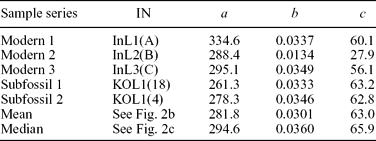
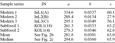
First, the predetermined growth trend function can be individually fitted to each series. Previous studies on M. margaritifera (Dunca, Reference Dunca1999; Helama & Valovirta, Reference Helama and Valovirta2008; Helama, Nielsen & Valovirta, Reference Helama, Nielsen and Valovirta2007; Helama & Nielsen, Reference Helama and Nielsen2008) have demonstrated that a suitable growth trend can be produced using the modified negative exponential function of Fritts, Mosimann & Bottorff (Reference Fritts, Mosimann and Bottorff1969). This is

where a determines the initial height of the curve, b controls the concavity of the function, c is the terminal height of the curve and x is the time from the first observable increment to the last measured increment number. Since the growth trends are fitted individually to each series, the method and resulting sclerochronologies are referred to hereafter as IND.
Alternatively, the growth trend model could be fitted to the summary ageing curve of all available series. In this method, the sample series were at first aligned according to their incremental years (instead of calendar years) and summary curve produced (by averaging or by the median). The summary curve was modelled using Eq. (1) to obtain the expected growth trend as a function of biological age. As this curve could be deciphered as a regional ageing curve for the species, Briffa et al. (Reference Briffa, Jones, Schweingruber, Karlén, Shiyatov, Jones, Bradley and Jouzel1996) termed the method ‘regional curve standardization’ (RCS).
Once the expected IND and RCS growth trends were determined, they were subsequently removed from the individual series by calculating the resulting sclerochronological indices as ratios between the observed and expected increment values. Thereafter, the index series were to be combined into the IND and RCS sclerochronologies. This is commonly done by averaging the annual index values using the arithmetic mean. Alternatively, the use of the biweight robust mean (Mosteller & Tukey, Reference Mosteller and Tukey1977) could improve the chronology estimation in the presence of non-climatic growth disturbances, as proposed by tree-ring studies (E. R. Cook, unpub. Ph.D. thesis, Univ. Arizona, 1985). In addition, if the sample size drops below six series, as in many sclerochronological studies as well as here, the biweight robust mean estimation could be replaced simply by the median (Mosteller & Tukey, Reference Mosteller and Tukey1977; Cook, Shiyatov & Mazepa, Reference Cook, Shiyatov, Mazepa, Cook and Kairiukstis1990). Accordingly, we evaluated the climate sensitivities of the mean (MEAN) and the median (MD) based sclerochronologies and, therefore ran the analyses using alternative sclerochronologies, IND–MEAN, IND–MD, RCS–MEAN and RCS–MD, all four initiating from the very same, but differently treated, sample series. In the case of RCS–MD, both the summary curve for ageing and the chronology were estimated using the median instead of the arithmetic mean.
2.c. Evaluating the proxy–climate relationships
This proxy–climate study was complemented by instrumental temperature observations already made in parts of northern Fennoscandia since ad 1802 (Holopainen, Reference Holopainen2006). Using the available multi-station climatic dataset, Klingbjer & Moberg (Reference Klingbjer and Moberg2003) developed a continuous air temperature series with monthly means from ad 1802 to 2002. This record was adopted here as an estimate of temperature variations in the region. Correlations between the annual shell growth increments of live-collected M. margaritifera and climate have previously been studied among Swedish populations (Mutvei et al. Reference Mutvei, Westermark, Dunca, Carell, Forberg and Bignert1994; Dunca, Reference Dunca1999; Schöne et al. Reference Schöne, Dunca, Mutvei and Norlund2004; Dunca, Mutvei & Schöne, Reference Dunca, Mutvei and Schöne2005). According to these studies, the annual shell growth was positively correlated with summer temperatures in Swedish rivers with decreasing climatic correlation in polluted environments. Correspondingly, we compared the growth variations to mean temperatures of the summer months only. In the study region, M. margaritifera typically dwells in small and extremely shallow streams (Oulasvirta, Reference Oulasvirta and Oulasvirta2006) where water temperature variations are likely to be strongly correlated with air temperatures through the ice-free season in summer.
The strength of association between proxy and climate was evaluated using the Pearson product–moment correlation coefficient, which is a measure of statistical agreement that describes the linear relationship between two series. The proxy–climate correlations were computed separately for the original series (that is, non-filtered climate data and sclerochronologies) and for series that were filtered to emphasize the low-frequency variations in proxy and climate series (‘low-pass’ filtering). In order to emphasize the low-frequency band of the variations in sclerochronological data and climate, the series were smoothed using a 25-year cubic spline function with 50% cut-off (Cook & Peters, Reference Cook and Peters1981). That is, the low-pass filtered series will exhibit variations on timescales of a decade and longer only. Since the natural time series are likely to contain markedly high autocorrelations (especially the low-pass filtered series), the significance levels of the correlations cannot be adopted from standard tables in statistical textbooks. One thousand Monte Carlo simulations (Efron & Tibshirani, Reference Efron and Tibshirani1986) were performed in the case of each correlation calculation to produce surrogate series that mimicked the autocorrelation structure present in the actual series. The empirical probability distribution of each statistic was then used to estimate the significance.
3. Results
3.a. Shells and their incremental series
The original study material contained three shells from the modern death assemblage and three unearthed shells from the subfossil death assemblage. The shells were all affected by fragmentation and dissolution to a different degree (Nielsen, Helama & Nielsen, Reference Nielsen, Helama and Nielsen2008). Subfossil samples number 1 and 2 were less affected by the umbonal dissolution than shell sample number 3 (Fig. 1). That is, the latter specimen exhibited umbonal dissolution on a much wider area of the shell surface than in other shells.
Three shells from the subfossil death assemblage and their incremental series: (a) left valve of sample number 1, (b) right valve of sample number 2, (c) left valve of sample number 3; sample series of the annual shell growth increments of (d) sample number 1, (e) sample number 2 and (f) sample number 3. Umbo was most extensively corroded in shell sample number 3. Series of growth are aligned according to the increment number counted from the umbo onwards.

It was found that the loss of the umbonal increments had considerable influence on the resulting increment width series of that particular sample. While samples 1 and 2 exhibited a clear growth trend with exponential decline of increment width towards the biologically older increments (Fig. 1d, e), it was not possible to observe a trend of any kind in sample series number 3 (Fig. 1f). This was obviously due to loss of biologically young increments via dissolution. In order to avoid any kind of bias in the estimation of mean growth trend and resulting sclerochronological indices, sample number 3 was excluded here from the further analyses. The remaining set of five sample series showed growth trends of similar overall features (Fig. 2a).
(a) Comparison of growth in selected five sample series as a function of ontogeny. Trend in the summary ageing curves calculated by (b) mean and (c) median, modelled using negative exponential function (Eq. 1).

The IND indices were derived from the modelled growth trends fitted individually to each series (Table 1). The RCS indices were derived from the empirically determined growth trend that was obtained as an ageing model of the mean (Fig. 2b; Table 1) and the median summary curves (Fig. 2c; Table 1). Mean inter-series correlations, calculated as a mean correlation between all overlapping pairs of index series from five shells, were 0.461 and 0.423 for the resulting IND and RCS series, respectively.
3.b. Sclerochronologies
Differently produced sclerochronologies correlated positively and notably strongly with each other in visual comparison (Fig. 3a). The view was quantified by statistical comparisons. Strong and positive correlations were found for non-filtered chronologies, containing the full spectrum of growth variability (Table 2a), and also for low-pass filtered chronologies that emphasize the growth variability on timescales of a decade and longer (Table 2b). However, a closer look at the correlations revealed decreasing similarity when the low-pass filtered IND and RCS chronologies were compared (Table 2b). This would indicate that the chronologies showed deviating growth variability, particularly on long timescales, likely due to methodology that was used to remove the growth trends. In light of this, the low-frequency components of the chronologies were compared in more detail. It was found that both types of RCS chronologies showed notably lower and higher index values before and after the 1870s, respectively, compared to the IND chronologies. This basic difference was apparent both for MEAN (Fig. 3b) and MD chronologies (Fig. 3c). In other words, the RCS chronologies contained an ascending long-term trend that was missing in both IND chronologies.
Comparison between the differently produced sclerochronologies (a) before and (b, c) after low-pass filtering. Statistical correlations of the chronologies are presented in Table 2.

Pearson correlations between the differently produced sclerochronologies

Correlations were calculated between (a) non-filtered and (b) low-pass filtered chronologies, over the period ad 1802–1979.
3.c. Climate signals
Notably strong proxy–climate correlations were found when the sclerochronologies were compared to mean temperatures of July, August and the July–August period. All four chronologies correlated positively and statistically significantly (p < 0.001) with the summer temperature variations. Overall, the highest proxy–climate fidelity was obtained between the shell growth and July–August temperatures in the case of all chronologies. It is notable that chronologies showed only negligible differences in the climatic correlativity when the non-filtered series (containing the full spectrum of variability) were compared (Fig. 4).
Pearson correlations between the differently produced sclerochronologies and mean temperatures (ad 1802–1979) of July (JUL), August (AUG) and July–August period (JUL–AUG), calculated using the non-filtered series. All correlations were statistically significant (p < 0.001).

Quite a different view was generated by the comparison of the low-frequency components of the proxy and climate variability. While the IND–MEAN and IND–MD chronologies exhibited no statistically significant climatic correlations (Fig. 5a, b), notably increased low-frequency fidelity was found in the case of both RCS chronologies. More specifically, RCS–MEAN correlated significantly (p < 0.05) with July and July–August temperatures (Fig. 5b, c). Even more improved proxy–climate associations were found for the RCS–MD chronology that correlated significantly with July and August temperatures (p < 0.05), as well as with July–August temperatures (p < 0.01) (Fig. 5c). Therefore, the chronology that served as the most reliable proxy for the summer temperature variations was RCS–MD (Fig. 6).
Pearson correlations between the differently produced sclerochronologies and mean temperatures (ad 1802–1979) of July (JUL), August (AUG) and July–August period (JUL–AUG), calculated using the low-filtered series.

Total variability in the mean July–August temperatures and RCS–MD sclerochronology. The proxy–climate correlation between the years 1802 and 1979 was 0.548.

4. Discussion
4.a. Shell alteration via pre-mortem and post-mortem taphonomy
Sclerochronological studies are based either on biological or palaeontological material. Live-collected shell specimens provide information about the recent growth variations with known post-mortem age, but palaeontologists seek to understand better the natural variations in the past. This requires access to ancient shell material. Such material can be retrieved either from geological (Kidwell, Reference Kidwell, Allison and Briggs1991) or archaeological deposits (Bar-Yosef Mayer, Reference Bar-Yosef Mayer and Bar-Yosef Mayer2005). The presently studied species, Margaritifera margaritifera, carries pearls in some of the shells, and the species has accordingly been ‘hunted’ in northern Finland and Lapland for several centuries (Lönnroth, Reference Lönnroth1941; Brander, Reference Brander1956; Montonen, Reference Montonen and Linkola1985). The presence of dorso-posterior fractures in many shells would suggest the use of a knife to open the shells by cutting adductor muscles (Nielsen, Helama & Nielsen, Reference Nielsen, Helama and Nielsen2008). This evidence would point to pearl hunting as an origin of the deposits (Helama, Nielsen & Valovirta, Reference Helama, Nielsen and Valovirta2007; Nielsen, Helama & Nielsen, Reference Nielsen, Helama and Nielsen2008). Accordingly, pearl hunting may actually have increased the likelihood of finding ancient shell material in the region (Helama & Nielsen, Reference Helama and Nielsen2008).
Whether geological or archaeological shell material is studied, the taphonomical processes influence the shells as the post-mortem conditions alter the material via dissolution, bioerosion, abrasion, disarticulation and fragmentation (Nielsen, Reference Nielsen2004). The shells of unionids, including M. margaritifera, are composed of aragonite (Compere & Bates, Reference Compere and Bates1973; Carell et al. Reference Carell, Dunca, Gärdenfors, Kukakowski, Lindh, Mutvei, Nyström, Seire, Slepukhina, Timm, Westermark and Ziuganov1995; Liao et al. Reference Liao, Mutvei, Sjöström, Hammarström and Li2000) that is rather soluble in freshwater environments undersaturated with respect to carbonates (Cummins, Reference Cummins1994). As a result, the dissolution of unionid and especially M. margaritifera shell is known to begin already with pre-mortem taphonomical processes (Linné, Reference Linné and Gmelin1806; Björk, Reference Björk1962; Cummins, Reference Cummins1994; Helama & Valovirta, Reference Helama and Valovirta2007). One of our subfossil shells contained a prismatic layer with extensive dissolution (Fig. 1c). This in turn had implications for the resulting incremental series and their analyses. Dissolution had affected mainly the umbonal shell region that contains the juvenile increments. The first and supposedly the widest increments of that specimen were lost, and the series did not exhibit the growth trend that was typical of all the other series in this study (Figs 1d, e, 2a). As noted above, the possibility of incomplete increment series may complicate the construction of RCS chronologies from taphonomically altered shells, especially when the chronology comprises a small number of sample series, as is the case here. First, if the series with an incomplete growth trend are used in the analyses, these series could bias the summary curve and ageing models and thus bias the resulting indices and the final RCS chronologies. On the contrary, it could be assumed that incomplete growth trends would not have a similar biasing influence on the IND chronologies, since in this method the growth trend models are fitted individually to each series. Therefore, one could expect the IND method to be better suited to sclerochronological studies that employ shell material with well-progressed taphonomical alteration (e.g. dissolution and fragmentation). Here, the shell with extensive alteration was excluded from both IND and RCS chronologies to facilitate sclerochronological comparisons with an identical dataset. Interestingly, the umbonal dissolution of the shell and its potential influence on the RCS method is similar to dendrochronological problems relating to pith offset (a number of rings missing in a tree-ring sample series near the pith) (Esper, Cook & Schweingruber, Reference Esper, Cook and Schweingruber2002; Esper et al. Reference Esper, Cook, Krusic, Peters and Schweingruber2003). In the dendrochronological context, the pith offset has not been found to be a major problem in biasing RCS based index series (Esper et al. Reference Esper, Cook, Krusic, Peters and Schweingruber2003), however, the sample size is commonly much higher in tree-ring studies compared to sclerochronology, and this may have mitigated its impact.
Moreover, the area of prismatic dissolution extends progressively through the lifespan of the mussels (Helama & Valovirta, Reference Helama and Valovirta2007). That is, the older the mussel, the larger the area of dissolution on and near the umbo, as a rule of thumb. As a consequence, one could expect to find more juvenile increments lost in ontogenetically older specimens than in younger and to observe differentiated growth trends as a function of pre-mortem taphonomy owing to biological age of the shells. Therefore, we emphasize the importance of comparing the growth trends of the mussels of different biological ages, before computing the growth trend models, in order to avoid any age-related bias when determining the empirical summary curves for ageing. Alternatively, one could apply the methods provided in literature to estimate the number of lost increments (e.g. Hendelberg, Reference Hendelberg1960; Bauer, Reference Bauer1992; Helama & Valovirta, Reference Helama and Valovirta2007), and build the growth trend models using the adjusted ontogenetic ages that would account for the umbonal dissolution. In actual fact, one of these methods (Helama & Valovirta, Reference Helama and Valovirta2007) was tested on the present material to estimate the number of the dissolved juvenile increments (results not shown). However, compared to the RCS chronologies constructed using unadjusted increment ages, the chronology built by adjusted ontogenetic ages showed only insignificant differences. This was, as mentioned above, likely the case, since the studied set of shells belonged to same age class of mature mussels.
Apart from biological age, the rate of pre-mortem dissolution in M. margaritifera shells is likely influenced by river water chemistry (Björk, Reference Björk1962). In the case of multi-river studies and partially dissolved bivalve shells, it would be important to compare river-specific growth trend models for detrending (as we actually did since our shells were all from the same river) or at least using specimens from waters of similar chemistry, when building the growth trend models for detrending purposes. As known from tree-ring studies, data heterogeneity may well be one of the most likely origins of biased chronology values (Briffa et al. Reference Briffa, Jones, Schweingruber, Karlén, Shiyatov, Jones, Bradley and Jouzel1996; Esper et al. Reference Esper, Cook, Krusic, Peters and Schweingruber2003; Helama et al. Reference Helama, Timonen, Lindholm, Meriläinen and Eronen2005). In the context of freshwater bivalves, alterations in water chemistry may result in such heterogeneity with potential influences on sclerochoronological RCS implementation.
4.b. Exploiting the annual increments
Chronological control of skeletal diaries can be validated and consequently improved if the procedure of cross-dating is applied to data. In our example, the sclerochronological cross-dating of the increment series verified the temporal control of each increment at annual resolution (Helama & Valovirta, Reference Helama and Valovirta2008; Helama, Nielsen & Valovirta, Reference Helama, Nielsen and Valovirta2008). The concepts and numerical approaches of sclerochronological cross-dating are to a great extent inherited from dendrochronological studies. Dendrochronology has applied the technique to tree-rings for a much longer time (Douglass, Reference Douglass1941; Fritts, Reference Fritts1976) and in fact, dendrochronologists restrict the term dendrochronology to refer only to material or studies to which careful cross-dating has been successfully applied (Fritts, Reference Fritts1976). Following this dendrochronological concept, a reasonable goal of any sclerochronological study would be to apply cross-dating to skeletal diaries to assure their fine-scale temporal control (Helama et al. Reference Helama, Schöne, Black and Dunca2006). Using this more precise terminology, our study material fulfils the criteria for high-quality sclerochronology.
The molluscan sclerochronologies published so far, that have been rigorously cross-dated (Marchitto et al. Reference Marchitto, Jones, Goodfriend and Weidman2000; Strom et al. Reference Strom, Francis, Mantua, Miles and Peterson2004, Reference Strom, Francis, Mantua, Miles and Peterson2005; Epplé et al. Reference Epplé, Brey, Witbaard, Kuhnert and Pätzold2006; Helama et al. Reference Helama, Schöne, Black and Dunca2006, Reference Helama, Schöne, Kirchhefer, Nielsen, Rodland and Janssen2007; Scourse et al. Reference Scourse, Richardson, Forsythe, Harris, Heinemeier, Fraser, Briffa and Jones2006; Helama, Nielsen & Valovirta, Reference Helama, Nielsen and Valovirta2007, Reference Helama, Nielsen and Valovirta2008; Helama & Valovirta, Reference Helama and Valovirta2008), have virtually all been based on the annual banding in bivalve shells. Similarly, the chronological control of coral records has previously been ensured by comparison of anomalous annual bands in different sites to identify and date the growth disturbances and hiatus (Hudson et al. Reference Hudson, Shinn, Halley and Lidz1976; Hendy, Gagan & Lough, Reference Hendy, Gagan and Lough2003; Hendy, Lough & Gagan, Reference Hendy, Lough and Gagan2003). Moreover, Black, Boehlert & Yoklavich (Reference Black, Boehlert and Yoklavich2005) cross-dated the annual growth increments in long-lived fishes to cross-date the series of Sebastes diploproa otoliths, similarly to techniques applied in sclerochronology and dendrochronology. Clearly, the incremental cross-dating of annually banded records is gaining ground as a high-precision dating tool in geochronology and is expected to bring significant advances over the coming years (Walker, Reference Walker2005). While the increment series yield temporally high-resolution palaeoenvironmental archives, it ought to be stressed that only rigorous cross-dating, albeit tedious in practise, is able to ensure the actual annual temporal control of these series.
4.c. Detrending method and low-frequency variations
Annual increment data are, in the first instance, biological series. Molluscan ontogeny influences the growth variability and results in a non-climatic trend throughout the lifespan of each individual (Fig. 2; Table 1). Since only the climate is considered to be a desired signal in palaeoclimatic studies, detrending is targeted to remove all other variations from increment width series except the climatic growth component. An important caveat in this respect is that detrending may remove not only the non-climatic growth variations but also the actual climatic signal, especially when the latter operates on similar timescales relative to trend (Fritts, Reference Fritts1976; Cook et al. Reference Cook, Briffa, Meko, Graybill and Funkhouser1995). Accordingly, it is particularly difficult to obtain sclerochronological growth indices containing the low-frequency variations of past climates and, as it is known from tree-ring studies, the methods applied in removing the non-climatic variations from the initial growth series may appreciably influence the interpretation of variation in past and present climates, especially at low frequencies (Cook et al. Reference Cook, Briffa, Meko, Graybill and Funkhouser1995; Briffa et al. Reference Briffa, Jones, Bartholin, Eckstein, Schweingruber, Karlén, Zetterberg and Eronen1992, Reference Briffa, Jones, Schweingruber, Karlén, Shiyatov, Jones, Bradley and Jouzel1996; Esper et al. Reference Esper, Cook, Krusic, Peters and Schweingruber2003; Helama et al. Reference Helama, Lindholm, Timonen and Eronen2004, Reference Helama, Timonen, Lindholm, Meriläinen and Eronen2005). This would be particularly unfortunate since there is a growing need to reconstruct the low-frequency variations in past climates (Esper, Cook & Schweingruber, Reference Esper, Cook and Schweingruber2002; Moberg et al. Reference Moberg, Sonechkin, Holmgren, Datsenko, Karlén and Lauritzen2005). Undoubtedly, the need to unveil particularly the low-frequency variations in past climates is an important element in palaeontological shell growth increment analyses.
Here we applied two approaches of growth trend modelling that were previously evaluated to be capable of retaining the low-frequency growth variability in the dendrochronological context (Briffa et al. Reference Briffa, Jones, Bartholin, Eckstein, Schweingruber, Karlén, Zetterberg and Eronen1992, Reference Briffa, Jones, Schweingruber, Karlén, Shiyatov, Jones, Bradley and Jouzel1996; Cook et al. Reference Cook, Briffa, Meko, Graybill and Funkhouser1995, Reference Cook, Briffa, Cook and Kairiukstis1990; Lindholm, Reference Lindholm1996; Esper et al. Reference Esper, Cook, Krusic, Peters and Schweingruber2003; Helama et al. Reference Helama, Lindholm, Timonen and Eronen2004). These models were those working on a deterministic (sensu Cook et al. Reference Cook, Briffa, Shiyatov, Mazepa, Cook and Kairiukstis1990) and an empirical (sensu Cook et al. Reference Cook, Briffa, Meko, Graybill and Funkhouser1995) basis. First, a predetermined growth trend model (Eq. 1) was fitted individually to each series and the trend expected by this curve was removed to derive IND index series and chronologies. Secondly, an empirically determined growth trend model was estimated as the mean (Fig. 2b) and the median summary curves (Fig. 2c) describing the ageing of the mussels. The ageing curves were modelled (Eq. 1) to remove this component from the initial increment width series, thus transforming them into RCS index series and chronologies. It was shown that the RCS chronologies contained more low-frequency variations and that the RCS chronologies correlated markedly better with the climate variability on low frequencies than the IND chronologies (Fig. 5). The low-frequency correlations between the IND chronologies and climate were in fact found to be statistically non-significant. Importantly, both of these findings were parallel to previous dendrochronological studies showing that the RCS chronologies have potential to preserve the low-frequency growth variations. As stated by Cook et al. (Reference Cook, Briffa, Meko, Graybill and Funkhouser1995), the RCS method allows for climatic low-frequency changes in the chronology, since the level of growth during any period may be systematically over- or underestimated by the ageing model because of changing external (climatic) conditions.
In a sclerochronological context, Strom et al. (Reference Strom, Francis, Mantua, Miles and Peterson2005) experimented using the RCS method in detrending the annual shell growth increment series of the marine geoduck clam, Panopea abrupta, sampled near Protection Island, coastal British Columbia. Similarly to our study, they compared the deterministic (analogous to our IND) and empirical (analogous to our RCS) detrending methods and found that their RCS chronology exhibited enhanced spectral power at periods exceeding the length of growth segments (Strom et al. Reference Strom, Francis, Mantua, Miles and Peterson2005). This result was very similar to our finding showing that the M. margaritifera RCS chronologies were found to contain long-term variation absent in IND chronologies (Fig. 3b, c). Further, the low-frequency variations preserved in our RCS chronologies were strongly correlative to observed long-term warming in the climate record (Fig. 6). Proxy–climate comparison by Strom et al. (Reference Strom, Francis, Mantua, Miles and Peterson2005) showed that their RCS chronology provided stronger correlation with coastal air-temperatures than the IND chronology during the earliest portion of the chronology. However, the proxy–climate correlations were essentially identical over the full ad 1850–1999 period (Strom et al. Reference Strom, Francis, Mantua, Miles and Peterson2005). Interestingly, as it was also shown here, the IND and RCS chronologies correlated with nearly identical coefficients with the climate variability when the full range of variations were compared (Fig. 4). However, it was particularly the low-frequency comparison that revealed the benefit of using the RCS method, because of improved proxy–climate correlations regarding the long-term and long-period variations in particular (Fig. 5).
In the foreseeable future, more studies will likely concentrate on the low-frequency issues in sclerochronologies from a variety of habitats and species. Available studies so far from both marine (Strom et al. Reference Strom, Francis, Mantua, Miles and Peterson2005) and freshwater (this study) realms making use of RCS have found that the method may indeed provide some benefits in assessing the past climate variations on scales of 10+ years. It is notable, however, that the RCS method is more sensitive to sample age (biological and geological) than the IND method (Cook et al. Reference Cook, Briffa, Meko, Graybill and Funkhouser1995; Briffa et al. Reference Briffa, Jones, Schweingruber, Karlén, Shiyatov, Jones, Bradley and Jouzel1996; Helama et al. Reference Helama, Timonen, Lindholm, Meriläinen and Eronen2005). If the sample ages of live-collected shells are very similar to each other, there is a risk that the empirical growth trend model will contain much climatic variation that will then be inadvertently removed in detrending. Similar problems were mentioned in a dendrochronological context by Briffa et al. (Reference Briffa, Jones, Schweingruber, Karlén, Shiyatov, Jones, Bradley and Jouzel1996). If, however, the samples originate over long periods of time, there is a risk that the very-low-frequency background variability in environmental conditions (e.g. long-term changes in catchment erosion, availability of food or population density) may change the behaviour of the non-climatic growth trend of the molluscs. This would lead to serious problems involving the assumption that the empirical growth curve represents the true ontogenetic curve over long periods of time (Helama et al. Reference Helama, Timonen, Lindholm, Meriläinen and Eronen2005). These issues demonstrate the paradox of the RCS method that is to be fully explored in the context of sclerochronology in the near future.
4.d. Mean and median as summary statistics
The arithmetic mean and the median are summary statistics with differing properties. While changing a small part of the body of data may change the value of the mean substantially, the median is the prototype of a resistant summary statistic (Mosteller & Tukey, Reference Mosteller and Tukey1977). In the context of natural time-series, such as tree-rings and annual shell growth increments, the importance of resistance in estimating variation among the populations lies in the potential existence of outlier indices in one or more of the individual sample series (E. R. Cook, unpub. Ph.D. thesis, Univ. Arizona, 1985). Nevertheless, the arithmetic mean is a commonly used summary statistic in sclerochronological studies published up to now. Here the two approaches were used to construct chronologies and these sclerochronologies were compared with climate data. It was found that the proxy–climate correlations were nearly identical when the full spectrum of variations in the two types of series were compared (Fig. 4). However, the low-frequency comparison of the proxy and climate series indicated that the RCS–MD chronology correlated markedly better with July and August as well as July–August temperatures than the RCS–MEAN chronology (Fig. 5c). In conclusion, the chronology which served as a proxy that most reliably mimicked the summer temperature variations in the region, taking into consideration both the high and the low frequencies, was RCS–MD (Fig. 6).
Compared to the arithmetic mean and the median, a yet more sophisticated summary statistic is the biweight robust mean (Mosteller & Tukey, Reference Mosteller and Tukey1977). It is calculated by iteration and, similarly to the median, it is more resistant to outliers than the arithmetic mean. Moreover, its usefulness has previously been demonstrated in the dendrochronological context (E. R. Cook, unpub. Ph.D. thesis, Univ. Arizona, 1985; Cook, Shiyatov & Mazepa, Reference Cook, Shiyatov, Mazepa, Cook and Kairiukstis1990). According to Mosteller & Tukey (Reference Mosteller and Tukey1977), the biweight robust mean outperforms the arithmetic mean in small or large samples. Likewise, the biweight robust mean also outperforms the median in the case of a large sample size. Here we used the median, since it has been previously recommended that the median should replace the biweight robust mean when the sample size falls below six (Mosteller & Tukey, Reference Mosteller and Tukey1977; Cook, Shiyatov & Mazepa, Reference Cook, Shiyatov, Mazepa, Cook and Kairiukstis1990). Accordingly, it could be recommended that future sclerochronological research should explore the influences of different summary statistics more thoroughly than has been done in the past.
4.e. Chronology sample size and reliability
Sample size is probably the simplest measure of chronology quality. Many of the longest molluscan sclerochronologies published so far have been characterized by relatively small sample size. For example, Marchitto et al. (Reference Marchitto, Jones, Goodfriend and Weidman2000) constructed a composite sclerochronology for southeastern Georges Bank, southeast off the coast of New England (USA), using three live collected and four dead-collected shells of ocean quahog, Arctica islandica. Sclerochronologically cross-dated shells were connected to span the interval from ad 1865 to 1994, but the pre-1900 part of the chronology resulted from a single shell-specific series (Marchitto et al. Reference Marchitto, Jones, Goodfriend and Weidman2000). Later, Scourse et al. (Reference Scourse, Richardson, Forsythe, Harris, Heinemeier, Fraser, Briffa and Jones2006) were able to construct a 267-year sclerochronology using the annual increment series of A. islandica, from the northern North Sea, that covered the period roughly from ad 1000 to 1400 (based on additional radiocarbon dating). However, the chronology of Scourse et al. (Reference Scourse, Richardson, Forsythe, Harris, Heinemeier, Fraser, Briffa and Jones2006) consisted of no more than three shell-specific incremental series. By contrast, recent advancements in tree-ring science have resulted in regional collections of dendrochronological material that comprise hundreds to thousands of sample-specific series of subfossils (Spurk et al. Reference Spurk, Leuschner, Baillie, Briffa and Friedrich2002; Eronen et al. Reference Eronen, Zetterberg, Briffa, Lindholm, Meriläinen and Timonen2002). In the context of these examples, our sample set mimicked the characteristics of the published palaeontological shell collections (e.g. Marchitto et al. Reference Marchitto, Jones, Goodfriend and Weidman2000; Scourse et al. Reference Scourse, Richardson, Forsythe, Harris, Heinemeier, Fraser, Briffa and Jones2006) in terms of sample quantity.
Another yardstick for chronology quality is the mean inter-series correlation that measures the common growth signal (Wigley, Briffa & Jones, Reference Wigley, Briffa and Jones1984; Briffa & Jones, Reference Briffa, Jones, Cook and Kairiukstis1990). As calculated above, the mean inter-series correlations of the IND and RCS index series were 0.461 and 0.423, respectively. The finding parallels the change in the mean inter-series correlations of tree-rings that are also known to change according to the detrending method (Fritts, Reference Fritts1976; Cook & Briffa, Reference Cook, Briffa, Cook and Kairiukstis1990; Helama et al. Reference Helama, Lindholm, Timonen and Eronen2004). Moreover, Helama et al. (Reference Helama, Schöne, Black and Dunca2006) calculated the mean inter-series correlations using a dataset of annual shell growth increments measured from the live-collected M. margaritifera that originated from one river in southern Sweden. They removed the growth trend from the initial shell growth increment series using detrending curves of varying flexibilities and found that the correlations commonly ranged between 0.425 and 0.450. Similar implications were previously drawn by Helama & Nielsen (Reference Helama and Nielsen2008) by studying a floating sclerochronology of M. margaritifera in which the IND index series showed a mean inter-series correlation with a coefficient of 0.52. Importantly, these findings (Helama & Nielsen, Reference Helama and Nielsen2008; this study) would indicate that these dead-collected chronologies (which originated from modern and subfossil death assemblages) were not significantly different in their strength of common growth signal compared to live-collected chronologies.
Wigley, Briffa & Jones (Reference Wigley, Briffa and Jones1984) combined the two measures of chronology quality, the sample size and the inter-series correlation, to formulate a more complex quantification of chronology quality. The expressed population signal (EPS) defines the similarity between the chronology (the composite of a finite number of sample indices) and the theoretical ‘infinitely replicated’ chronology (that is, an EPS of 1.0) for the appropriate inter-series correlation (Wigley, Briffa & Jones, Reference Wigley, Briffa and Jones1984; Briffa & Jones, Reference Briffa, Jones, Cook and Kairiukstis1990). A reference value for a reliable chronology is commonly taken as 0.85, and the data with the EPS exceeding that value could generally be thought to represent reliable mean growth variations (Wigley, Briffa & Jones, Reference Wigley, Briffa and Jones1984; Briffa & Jones, Reference Briffa, Jones, Cook and Kairiukstis1990). Previously, Witbaard, Duineveld & De Wilde (Reference Witbaard, Duineveld and De Wilde1997) applied the EPS statistic in the context of live-collected A. islandica shells and their annual growth increment series to demonstrate temporal variations in the reliabilities of their marine sclerochronologies. In addition, Helama & Nielsen (Reference Helama and Nielsen2008) used the EPS statistic to determine the minimum number of sample series needed for a statistically reliable sclerochronology. Consequently, the variability in chronology was found to be statistically reliable with sample replication in at least six series (Helama & Nielsen, Reference Helama and Nielsen2008).
Applying the EPS to our data with the given mean inter-series correlations (0.461 and 0.423) showed that the number of replications of sample series needed for statistically reliable IND and RCS chronologies would be seven and eight, respectively (Fig. 7a). It could also be theorized that the mean inter-series correlation of 0.532 would be needed for EPS to exceed 0.85 with a given sample size of five series, whereas a tenfold sample replication would require inter-series correlation as low as 0.102 to produce identical values of EPS (Fig. 7b). A higher number of M. margaritifera series would thus be expected to elevate the EPS to optimal level. Nevertheless, the proxy–climate evidence demonstrated a strong and statistically highly significant palaeotemperature signal, especially in the case of RCS chronologies (Figs 3–6). How much better proxy–climate correlations the chronology would have yielded with markedly improved samples is a matter for conjecture, but it would seem fair to argue that in the case of a carefully constructed chronology (via cross-dating, taphonomic inspection and evaluation of growth trend models and summary statistics), even a rather small sample size may result in variations that could be of some use in the context of palaeoclimatology. Variations in such chronologies should naturally be treated with the greatest caution and ideally interpreted only in concert with other available proxies.
Relationships between the expressed population signal (EPS) and the mean inter-series correlation among the number of sample series. (a) Sample sizes of 7 and 8 would be required for IND and RCS chronologies to obtain EPS-values exceeding 0.85 (horizontal dotted line) that is commonly taken as a reference value for a reliable chronology. (b) Computational associations between the EPS and the inter-series correlation with sample size of 5, 10 and 50.

5. Conclusions and implications
Unfortunately for palaeoclimatology-oriented palaeontologists, the conchological growth series do not carry pure signals of past climate. Instead, these series of incremental shell growth are imprinted by a mixture of signals of different origin. Many of the complexities relating to non-climatic growth trends and detrending are actually largely statistical and not restricted to sclerochronology, but similar issues have long been recognized in tree-ring science. Consequently, much of the related knowledge can be adopted from dendrochronological literature. Both sclerochronology- and dendrochronology-based palaeoclimatic studies are premised on the idea that the non-climatic variability can somehow be separated from that produced by past climatic perturbations. A common procedure to do this is a statistical approach to determine an expected non-climatic growth trend for individuals or populations and accept the residuals from the expected curve as the climate signal. While the apparent benefit of these methods is their relative simplicity, the disadvantage comes along with the difficulty to evaluate how well one is really able to determine the actual non-climatic growth trend for each shell, or for a population of bivalves. Namely, if the expected trend contains a climatic component, the very same components are inadvertently removed in the detrending process. Moreover, since the biological growth trends influence the entire lifespan of the bivalve, from the first to last increment, it is particularly difficult to separate the climatic signals from those biological influences that operate on timescales that approximate or exceed the series lengths. This is also the simple explanation of why it is so difficult to remove the non-climatic variability but retain the low-frequency palaeoclimate signal in sclerochronological (and dendrochronological) datasets. One more complication comes from the relatively small sample size that is characteristic of many sclerochronological data, especially those originating from death assemblages of fossil or subfossil shells. In particular, the dendrochronological literature has pointed out the increasing difficulty of reconstructing the lowest frequencies of climate variability with decreasing sample sizes.
Here we applied two methods of growth trend modelling (here, IND and RCS) that were known as methodological trade-offs of building up expected growth trends that carry climatic variability to a lesser degree than some other statistical methods. Further, the skill of the arithmetic mean and the median as summary statistics to build the chronologies were assessed. Specifically, our analyses were carried out with a typical sclerochronological dataset consisting of sample series from shells few in number and discussed in the context of previous dendrochronological and sclerochronological studies. Similarly to previously published dendrochronological evidence, it was found that the sclerochronology-based RCS was likely more sensitive to small sample size and fragmentary growth series than the IND method. Concomitantly, we emphasized the value of compound interpretation via taphonomic analyses and growth trend modelling to achieve unbiased summary ageing curves needed in the RCS method. Subsequently, it was found that while the growth variability in all differently produced chronologies correlated significantly with the regional summer temperature variations, only the RCS chronologies were able to mimic the temperature variations at low frequencies (on timescales of decades and longer). Interestingly, it was found that the median served as an improved summary statistic. In conclusion, it could be deduced that the growth trend models produced by the RCS method contained less climatic information compared to IND curves and that the median was more insensitive to non-climatic growth perturbations than the mean. As a consequence, the RCS chronologies outperformed the IND chronologies at low frequencies and the median-based RCS chronology served as the most reliable version of the past growth variations.
Despite the recent progress in studying the skeletal increments of bivalves and other organisms, much more research is needed to increase the current understanding of the behaviour of sclerochronological data and the skeletal deposition under varying climate and environmental conditions. More knowledge will undoubtedly be gained with improved collections of live and dead shell materials and with the development of larger sclerochronological datasets. Meanwhile, the sclerochronologies in progress may, if constructed as well as evaluated by their signals with the greatest care, contribute to addressing the crucial need to augment the information about past climatic variations in freshwater and marine realms.
Acknowledgements
We are grateful to Dr Alan Wanamaker for comments that considerably improved this manuscript. WWF-Finland has supported the Margaritifera project. The Carlsberg Foundation kindly provided J.K.N. with a postdoctoral scholarship for a project (no. 04–0256/20). The shell samples were collected under the license from The Lapland Regional Environment Centre.