



1. Introduction
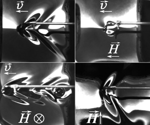
In nature, stationary waves behind an obstacle are observed in the oceans when storms and hurricanes move in the atmosphere (Svirkunov & Kalashnik Reference Svirkunov and Kalashnik2014) and on the water surface behind moving objects (Kelvin Reference Kelvin1906). The case of ship waves on a water surface has been studied in detail since Lord Kelvin's study (Thomson Reference Thomson1886). Analysis of these waves was based on the dispersion equation for gravity waves occurring on the water surface. A more detailed study of gravity waves continues at the present time (Darmon, Benzaquen & Raphaël Reference Darmon, Benzaquen and Raphaël2014; Pethiyagoda, McCue & Moroney Reference Pethiyagoda, McCue and Moroney2014). Waves on the surface of a thin film of a viscous fluid have been studied by Ledesma-Alonso et al. (Reference Ledesma-Alonso, Benzaquen, Salez and Raphaël2016). After Wilton (Reference Wilton1915), the attention of researchers focused on the peculiarities of formation of stationary gravity–capillary waves. This issue is at present being extensively studied both experimentally and theoretically (Moisy & Rabaud Reference Moisy and Rabaud2014; Liang & Chen Reference Liang and Chen2018; Gnevyshev & Badulin Reference Gnevyshev and Badulin2020; Flamarion & Ribeiro Reference Flamarion and Ribeiro2022).
The cause of the formation of stationary waves behind a moving obstacle (or a steady obstacle in a fluid flow) is dispersion, i.e. the dependence of the phase and group wave velocity on the wavelength. In magnetic fluids (ferrofluids), the dispersion equation (with the exception of common dispersion equations for the waves on a free surface) is determined by the magnetic field strength. Dispersion equations for deep water, for a layer of finite thickness, for a layer with two free boundaries and for other geometries can be found in Cowley & Rosensweig (Reference Cowley and Rosensweig1967), Zelazo & Melcher (Reference Zelazo and Melcher1969) and Berkovsky et al. (Reference Berkovsky, Medvedev and Krakov1993). These dispersion equations were confirmed experimentally by Barkov & Bashtovoy (Reference Barkov and Bashtovoy1977), Bercegol et al. (Reference Bercegol, Charpentier, Courty and Wesfreid1987), Reimann et al. (Reference Reimann, Richter, Knieling, Friedrichs and Rehberg2005) and Groh et al. (Reference Groh, Richter, Rehberg and Busse2007). But as far as we know, there are only three works devoted to stationary waves behind obstacles in magnetic fluids (Berkovsky et al. Reference Berkovsky, Bashtovoi and Krakov1980; Browaeys et al. Reference Browaeys, Perzynski, Bacri and Shliomis2001a,Reference Browaeys, Bacri, Perzynski and Shliomisb).
In Berkovsky, Bashtovoi & Krakov (Reference Berkovsky, Bashtovoi and Krakov1980), the effect of a magnetic field on the wave patterns was theoretically studied in the limiting cases of gravity waves in deep water and capillary waves in a thin liquid layer. It was shown that in these limiting cases the magnetic field parallel to the flow does not change the pattern of waves, but decreases the critical flow velocity above which the formation of stationary waves is possible. In this case, as the field increases, the wave crests approach the source, and at a sufficiently large field the stationary wave pattern is completely suppressed.
A field lying in the surface plane, which is perpendicular to the velocity, expands the wave cone angle. As a result, the crests of capillary waves on a thin layer transform from parabolas to hyperbolas, and in the presence of very strong magnetic fields the asymptote of these hyperbolas tends to become perpendicular to the magnetic field. In the case of gravity waves in a deep layer, the Kelvin angle increases, also tending to  ${\rm \pi}$/2, and thus we have a one-dimensional problem.
Wave resistance for gravity–capillary waves from a point source in a vertical magnetic field was studied in Browaeys et al. (Reference Browaeys, Bacri, Perzynski and Shliomis2001b). It was found that the critical flow velocity, above which the formation of stationary waves may occur, decreases, and the wave resistance increases according to the relation
 \begin{equation}R = \frac{{{R_0}}}{{\sqrt {1 - {{\left( {\frac{H}{{{H_\ast }}}} \right)}^2}} }},\end{equation}
where R 0 is the wave resistance in the absence of a magnetic field, H is the magnetic field strength and  ${H_\ast }$ is the critical value of the magnetic field above which the free surface of the magnetic fluid becomes unstable (Rosensweig instability). The fact that the magnetic field affects the wave resistance is supported by the results of the subtle experiment of Browaeys et al. (Reference Browaeys, Perzynski, Bacri and Shliomis2001a,Reference Browaeys, Bacri, Perzynski and Shliomisb).
To date, there are no theoretical or experimental data regarding the influence of a magnetic field on the gravity–capillary wave patterns created by a moving obstacle. This influence can differ significantly in all three cases of the magnetic field orientation relative to the direction of motion of the wave source.
2. Problem formulation and development of a method for its solution
A detailed explanation of the reasons for the formation of stationary waves initiated by a moving obstacle is given in Whitham (Reference Whitham1974). We here only briefly repeat these reasons to avoid any ambiguities. Let us suppose that, at some initial time, the source of perturbations, moving with velocity u, is at the point Q (figure 1), and at time t it reaches the point P. In order for the wave pattern to remain stationary relative to the source, the projection of the source velocity on the wave direction (vector  $\boldsymbol{k}$) must be compensated by the phase velocity of the wave c, i.e. the following equality must hold:
 \begin{equation}u\cos \psi = c.\end{equation}
Construction of wave elements in the stationary wave problem.

Since the phase velocity of a dispersive wave depends on the wavenumber k, this equality allows us to determine the value of k in the direction ψ.
The location of the wave crest T is determined by the group velocity cgr rather than by the phase velocity. For dispersive waves, these velocities are not equal, e.g. for gravity waves on water, cgr = c/2. If all points satisfying relation (2.1) are in the semicircle of radius PQ/2, then the stationary wave crests are in the semicircle of radii PQ/4 centred at the point R. It is therefore easy to understand (Lighthill Reference Lighthill1978) that, in the right triangle RTP, the maximum angle ξ at which the crests of stationary waves from the source are seen is determined by the relation
 \begin{equation}\sin \xi = \frac{{RT}}{{PR}} = \frac{1}{3},\end{equation}
which yields the known value of the half-angle of the Kelvin cone ξ = 19.47°.
Since the phase velocity c = ω 0(k)/k, relation (2.1) can be written as
 \begin{equation}uk\cos \psi - {\omega _0}(k) = G(k,\psi ) = 0,\end{equation}
where ω0(k) is the dispersion equation for the waves propagating on the surface of a motionless fluid.
In relation (2.2), the ratio RT/PR is determined by the relationship between the group and phase wave velocities, i.e. by their dispersion equation.
As is known, the dispersion equation for gravity–capillary waves in deep water has the form
 \begin{equation}{\omega _0}(k) = \sqrt {kg + \frac{{\sigma {k^3}}}{\rho }} ,\end{equation}
whence it is easy to find the minimum phase velocity of the waves:
 \begin{equation}{c_{min}} = \min \left( {\frac{{{\omega_0}}}{k}} \right) = \min \left( {\sqrt {\frac{g}{k} + \frac{{\sigma k}}{\rho }} } \right).\end{equation}
Then
 \begin{equation}c_{min}^2 = 2\sqrt {\frac{{\sigma g}}{\rho }} ,\quad {k_{min}} = \sqrt {\frac{{\rho g}}{\sigma }} .\end{equation}
These quantities are further used to determine the dimensionless wavenumber  $\hat{k}$ and the dimensionless velocity
 $\mathrm{{\mathcal U}}$:
 \begin{equation}\hat{k} = \frac{k}{{{k_{min}}}},\quad \mathrm{{\mathcal U}} = \frac{u}{{{c_{min}}}}.\end{equation}
Using (2.4) and (2.7a,b), we can rewrite expression (2.3) in dimensionless form:
 \begin{equation}\hat{G}(\hat{k},\psi ) ={-} 2\mathrm{{\mathcal U}}\hat{k}\cos \psi + \sqrt 2 \sqrt {\hat{k} + {{\hat{k}}^3}} = 0.\end{equation}
The locus of points that form the crests of stationary waves is determined by the group velocity. Therefore, according to Whitham (Reference Whitham1974), the crests of waves oriented at an angle  $\mu$ (figure 1) are located at a distance r from the moving obstacle:
 \begin{equation}r = \frac{\theta }{{k\cos \mu }},\end{equation}
where θ is the wave phase ( $\zeta \; = \; a\cos (kx - \omega t + \theta )$,
 $c = \omega /k$, a is the wave amplitude,
 $\zeta $ is the wave height). In this case, the angle
 $\mu$ can be calculated as (Whitham Reference Whitham1974)
 \begin{equation}\tan \mu = \frac{{\dfrac{1}{{\hat{k}}}\dfrac{{\partial \hat{G}}}{{\partial \psi }}}}{{\dfrac{{\partial \hat{G}}}{{\partial \hat{k}}}}}.\end{equation}
Thus, if the dispersion equation  ${\omega _0}(k)$ is known, then, given that
 $\xi = {\rm \pi}-\mu -\psi$, (2.8)–(2.10) allow us to find the coordinates of the wave crest points (r, ξ) in the polar coordinate system associated with the centre coinciding with the source of disturbances, where the angle ψ is used as a parameter.
3. Wave patterns of gravity–capillary waves in ordinary liquids
The roots of (2.8) have the form
 \begin{equation}{\hat{k}_{1,2}} = {\mathrm{{\mathcal U}}^2}{\cos ^2}\psi \pm \sqrt {{\mathrm{{\mathcal U}}^4}{{\cos }^4}\psi - 1} ,\end{equation}
and are real only for
 \begin{equation}\mathrm{{\mathcal U}} > 1.\end{equation}
The smaller root determines a pattern of the gravity branch of stationary waves and the larger root a pattern of the capillary branch. Depending on the value of  $\mathrm{{\mathcal U}}$, the pattern of crests changes. At values of
 $\mathrm{{\mathcal U}}$ close to unity, the capillary branch is located in front of the source, the gravity branch is behind it and the crest lines are close to the straight lines perpendicular to the velocity vector. As
 $\mathrm{{\mathcal U}}$ increases, the slope of the crests increases and, at
 ${\mathrm{{\mathcal U}}^\ast } \approx 1.938$, a cusp appears on the crest line of the gravity branch (figure 2b). With a further increase in the obstacle velocity, a second cusp occurs (figure 2c). These cusps are called the gravity (larger angle) and capillary (smaller angle) cusps, although both are on the gravity branch. Note that, up to
 $\mathrm{{\mathcal U}} \approx 3$, the regions of the capillary and gravity branches do not intersect, and at
 $\mathrm{{\mathcal U}} > 3$ both branches are inside the cone with angle
 $\alpha _g^{cusp}$, which tends to the Kelvin angle with increasing
 $\mathrm{{\mathcal U}}$ (figure 2c).
(a–c) Wave patterns (lines of isophase) at different flow velocities in dimensionless coordinates for the same phase: (a)  $\mathrm{{\mathcal U}} = 1.2$, (b)
 $\mathrm{{\mathcal U}} = 1.938$ and (c)
 $\mathrm{{\mathcal U}} = 6$. The arrows below the panels show the direction of movement of the obstacle. Here and further the red line refers to the capillary branch, the cyan line depicts the gravity branch and the green dashed line represents the demarcation line (equation (3.3)). The gravity cusp angle is shown in magenta, the capillary cusp line in blue and the Kelvin angle line in black. (d) Wave pattern on coloured water near the moving obstacle (experiment), u = 20 cm s−1; light areas correspond to the inclined surfaces of the wave and the dark areas correspond to the horizontal surfaces of the crests and troughs of stationary waves.

The angle of inclination of the demarcation line ξd, to which both the capillary and gravity branches asymptotically tend and which separates these branches up to  $\mathrm{{\mathcal U}} \approx 3$, is determined by the equality 0 of the radical expression in (3.1), i.e.
 ${\cos ^2}\psi = 1/{\mathrm{{\mathcal U}}^2}$. Moreover,
 $\hat{k} = 1$. In this case, expression (2.10) has the form
 $\tan \mu = 2(({\hat{k}^2} + 1)/({\hat{k}^2} - 1))\tan \psi$, and therefore
 $\tan \mu = \infty $. Since
 $\tan \xi = (\tan \mu + \tan \psi )/(\tan \mu \times \tan \psi - 1)$, then
 \begin{equation}\tan {\xi _d} = 1/\tan \psi = 1/\sqrt {{\mathrm{{\mathcal U}}^2} - 1} .\end{equation}
The linear theory shows the shape of the crests but does not provide information about the amplitude of the stationary waves. Nonlinear analysis (e.g. Moisy & Rabaud Reference Moisy and Rabaud2014) shows that the energy emitted by a moving source is accumulated along with the angles of the capillary and gravity cusps. However, for further analysis and meaningful comparison with the experiment carried out for velocities at which there were no cusps in the crest lines, the amplitude of stationary waves at  $\mathrm{{\mathcal U}} < 2$ is of greatest interest. As shown in figure 11 of Moisy & Rabaud (Reference Moisy and Rabaud2014), at low velocities, the inclination angle of a group of high-amplitude stationary waves is noticeably smaller than the inclination angle of the line demarcating the gravity and capillary branches ξd.
4. Experimental set-up and magnetic fluid
The experimental study of the gravity–capillary waves formed on a magnetic fluid free surface was carried out with a set-up shown schematically in figure 3. Two pairs of Helmholtz coils (1) were used to produce a magnetic field of either vertical (with radius R 1 = 122.5 mm and number of turns N 1 = 390) or horizontal (with radius R 2 = 97.5 mm and number of turns N 2 = 321) orientation. A cylindrical glass cell (2) of inner diameter D = 123.5 mm and sidewall height of 50 mm was placed on a horizontal platform in the centre of the Helmholtz coils. A magnetic field with a uniformity of at least 95 % in the central part of the coils (figure 4) was generated using a dual-channel stabilized Mastech DC power supply HY3010E-2B (3).
Scheme of the experimental set-up: 1, two pairs of Helmholtz coils, for the vertical and horizontal fields; 2, glass cell; 3, two-channel power supply; 4, milliteslameter; 5, resistor; 6, analogue-to-digital converter; 7, magnetic fluid; 8, stepper motor; 9, copper obstacle; 10, video camera; 11, mirror; 12, light source.

Relative distribution of the field strength along the radius of the Helmholtz coils R 1 (1) and R 2 (2). Vertical dashed lines mark the boundaries of the cuvette of diameter D = 123.5 mm (experiment). The inhomogeneity of the magnetic field in this cell did not exceed 5 %.

Magnetic field induction at the centre of the coil system was measured by a milliteslameter (4). The output signal from a small resistor (5), connected serially to the coils, was fed to the input of an analogue-to-digital converter ADC LA-I24 USB (6) and processed using a standard software kit. The obtained current I was recalculated using the values of the vertical magnetic field strength H, orthogonal to the fluid surface, according to the dependence H(I) kA m−1 = 1.0493I A, and H(I) kA m−1 = 1.1095I A for a horizontal magnetic field, tangential to the surface.
The cylindrical vessel was filled with a magnetic fluid (7). Layers of thickness h = 16 ± 1 mm and h = 30 ± 1 mm were used. A movable platform with a stepper motor (8), powered by a two-channel stabilized DC source (3), was placed in the working area in the horizontal plane from the sidewall of the vessel. The moving platform was rigidly connected to a smooth polished copper rod (9) of d = 1.5 mm in diameter and 300 mm long. The free end of the rod, bent at an angle of 90°, was immersed to a depth of 1–2 mm in the magnetic fluid, not touching the vessel bottom. The rod passed through two non-magnetic guide bushings spaced 30 mm apart – non-magnetic sleeve bearings. Any possible vibrations of the rod and the obstacle associated with it were damped by the guide bushings, as well as by the rigidity of the rod material. Thus, the rod played the role of a moving obstacle considered as a point. In this case, the Bond number was defined as  $Bo = d/{\lambda _c} = 0.2$ (where d is the rod diameter and
 ${\lambda _c}$ is the capillary wavelength,
 ${\lambda _c} = 2{\rm \pi}\sqrt {\sigma /\rho g} $) taking into account the properties of the magnetic fluid presented below. Since the Bond number is small, we use the point source approximation in the further analysis.
The velocity of the platform motion along with the obstacle was controlled using a Mastech current source. The voltage applied to the platform varied from 8 to 12 V, which made it possible to change the obstacle velocity in the range from 13.7 to 22.9 cm s−1.
The images of waves on the free surface of the liquid layer were captured by a Baumer TXG50 digital machine vision camera (Germany) (10) operating at a frame rate of 70 to 100 f.p.s. The pictures were obtained from both above and the side. For filming, a flat mirror (11) was installed above the coil system at an angle of 45° from the side. Visualization of the relief of the layer surface was performed using a circular LED light source (12).
In the experiments, we used a magnetic fluid of the type ‘magnetite + kerosene + oleic acid’, which was prepared by the standard method of chemical precipitation. The magnetic fluid density is ρ = (1753 ± 5) kg m−3 at ambient and working fluid temperatures (27 ± 1) °C. The dynamic viscosity of the fluid was determined using a Brookfield DV-II + Pro rotational viscometer, and it is expressed as η = (54 ± 1) mPa s at the same temperature. A magnetic fluid with such a high viscosity (and at the same time high magnetization) was chosen so that the wave pattern had an opportunity to stabilize at the very beginning of the obstacle movement. The surface tension of the ferrofluid measured by the standard ring tear-off method with a commercial Sigma 701 tensiometer (KSV Instruments Ltd) is σ = (25.7 ± 0.2) mN m−1.
The magnetization curve of the fluid (figure 5) was measured by the differential sweep method described in detail in Lebedev (Reference Lebedev1989). The saturation magnetization of the fluid is 72.74 kA m−1. The relative magnetic permeabilities  ${\mu _r} = \partial M/\partial H$ and
 ${\mu _s} = M/H$ were calculated from the magnetization curve (figure 6):
 \begin{align}\left. {\begin{array}{*{20}{c@{}}} {{\mu_r} ={-} 4.00 \times {{10}^{ - 12}}{H^3} + 1.28 \times {{10}^{ - 7}}{H^2} - 0.00151H + 8.79,\quad \delta = 1.75\,\%,}\\ {{\mu_s} ={-} 4.00 \times {{10}^{ - 12}}{H^3} + 1.15 \times {{10}^{ - 7}}{H^2} - 0.00128H + 8.79,\quad \delta = 2.34\,\%.} \end{array}} \right\}\end{align}
Here, H is measured in A m−1 and δ is the standard deviation. The volume concentration of magnetic particles covered with surfactant is 0.57, the dipole–dipole interaction parameter is estimated as λ = 0.8 and the average magnetic moment of the particle  $\langle m\rangle = 1.62 \times {10^{ - 19}}\textrm{ A}\;{\textrm{m}^2}$.
Magnetic fluid magnetization curve.

Magnetic permeabilities of magnetic fluid, where  ${\mu _r} = \partial M/\partial H,\;{\mu _s} = M/H$.

The photos (frames) obtained during the experiment were processed using the image processing software Comef 4.3 (OEG GmbH, Germany). The stationary wave crest tilt angles were measured depending on the magnitude and orientation of the applied magnetic field. By adjusting the position of the lighting device relative to the liquid surface and the parameters of brightness, contrast and exposure time of the camera during the experiment, the image of the wavefront can be obtained. For obstacle velocity exceeding 16 cm s−1, apart from the main crest of the wavefront (capillary branch), the gravity wave is seen in figure 7(a). For each frame, the wave cone angles were measured along several auxiliary lines (figure 7) and along the secondary waves, which are the trajectories of the liquid trace behind the moving obstacle. An example of stationary waves in a horizontal transverse magnetic field is presented in the supplementary movie available at https://doi.org/10.1017/jfm.2022.691.
Measurement scheme for the angles of the wave profile arising on the surface of a magnetic fluid near an obstacle moving from right to left at u = 20 cm s−1: (a) Hτ = 0; (b) Hτ = 5.5 kA m−1. The magnetic field is collinear to the velocity.

As a result, the final value of the measured angle for each frame was averaged over the entire dataset, the variance of which determined the measurement error. It should be noted that in the frame field the angles of inclination of the wave cone to the right and left relative to the obstacle (in figure 7, respectively, from above and from below) differed somewhat, which is associated with small deviations of the optical system from the vertical. However, the difference in the obtained angles of the wave cone on both sides relative to the obstacle does not in general exceed the statistical measurement error.
Hereinafter in the text of the paper, photos depict the view of the magnetic fluid free surface from above, and the direction of the obstacle movement is considered from right to left in the horizontal plane. In the presented images, the light areas correspond to the inclined surfaces of the wave and the dark areas correspond to the horizontal surfaces of the crests and troughs of stationary waves (figure 7a).
In the case of low obstacle velocity, as well as under the influence of a rather high magnetic field parallel to the velocity vector, the amplitude of stationary waves is very small. The wavefront is similar to a very small hemispherical surface in the vicinity of the obstacle (figure 7b). The measurement of angles, in this case, became almost impossible. Therefore, further experimental data are presented only for the wavefront in the form of cones (figure 7a).
5. Stationary waves in a vertical magnetic field
The surface of a magnetic fluid in a vertical magnetic field becomes unstable (Cowley & Rosensweig Reference Cowley and Rosensweig1967) when the magnetization of the fluid is greater than the critical one. This phenomenon is called the Rosensweig instability. The dispersion equation for linear waves obtained by Zelazo & Melcher (Reference Zelazo and Melcher1969) and for a deep layer (kh ≫ 1) has the form
 \begin{equation}{\omega _0}(k) = \sqrt {kg - \frac{{{\mu _0}M_n^2}}{{1 + 1/\sqrt {{\mu _r}{\mu _s}} }}\frac{{{k^2}}}{\rho } + \frac{{\sigma {k^3}}}{\rho }} ,\end{equation}
where Mn is the normal component of the fluid magnetization.
If, as before, kmin and cmin are defined as characteristic quantities, then we can write (5.1) in dimensionless form as
 \begin{equation}\hat{\omega }_0^2 = \hat{k} - \frac{{{\mu _0}M_n^2}}{{1 + 1/\sqrt {{\mu _r}{\mu _s}} }}\frac{1}{{\sqrt {\rho g\sigma } }}{\hat{k}^2} + {\hat{k}^3}.\end{equation}
The dimensionless complex  $({\mu _0}M_n^2/(1 + 1/\sqrt {{\mu _r}{\mu _s}} ))(1/\sqrt {\rho g\sigma } )$, which determines the onset of the Rosensweig instability, we call the Rosensweig number now, in the year of the 90th anniversary of Dr Ronald Rosensweig. In this study, the Rosensweig number is denoted by Ron.
The dispersion equation in its dimensionless form is as follows:
 \begin{equation}\hat{\omega }_0^2 = \hat{k} - R{o_n}{\hat{k}^2} + {\hat{k}^3}.\end{equation}
From (5.3) it follows that the frequency  $\hat{\omega }_0^2 > 0$ only for Ron < 2. The frequency
 $\hat{\omega }_0^2 = 0$ for Ron = 2,
 $\hat{k} = 1$, i.e. for Ron > 2,
 $\hat{\omega }_0^2 < 0$, and the surface is unstable in a vertical magnetic field; the most unstable wavelength is the wavelength corresponding to
 ${\hat{k}_{min}}$. However, at Ron < 2, the surface remains stable, and the motion of the obstacle across the surface may cause the formation of stationary waves. This wave resistance was discovered and measured by Browaeys et al. (Reference Browaeys, Bacri, Perzynski and Shliomis2001b). At the same time, the influence of the magnetic field on the shape of the crests of gravity–capillary waves remained unknown except for two special cases (Berkovsky et al. Reference Berkovsky, Bashtovoi and Krakov1980).
Using (5.3), (2.8) takes the form
 \begin{equation}\sqrt 2 \mathrm{{\mathcal U}}\hat{k}\cos \psi = \sqrt {\hat{k} - R{o_n}{{\hat{k}}^2} + {{\hat{k}}^3}} .\end{equation}
The solution to this equation is
 \begin{equation}{\hat{k}_{1,2}} = ({\mathrm{{\mathcal U}}^2}{\cos ^2}\psi + R{o_n}/2) \pm \sqrt {{{({\mathrm{{\mathcal U}}^2}{{\cos }^2}\psi + R{o_n}/2)}^2} - 1} .\end{equation}
Since the radical expression in (5.5) must be positive, the necessary condition for the formation of stationary waves is
 \begin{equation}\cos \psi > \cos {\psi ^\ast } = \sqrt {\frac{{2 - R{o_n}}}{{2{\mathrm{{\mathcal U}}^2}}}} .\end{equation}
Since the maximum value of cos ψ = 1, the existence of stationary waves is possible only at an obstacle velocity that satisfies the condition
 \begin{equation}\mathrm{{\mathcal U}} > \sqrt {1 - R{o_n}/2} .\end{equation}
Since the condition of the magnetic fluid surface stability Ron < 2 must be satisfied, we draw the obvious conclusion: the critical velocity, above which the formation of stationary waves is possible, tends to zero with increasing magnetic field. However, it should be remembered that the position of the crests is determined by the group velocity, which must be positive. According to (5.1), the group velocity of waves on the magnetic fluid surface is
 \begin{equation}\frac{{\partial {\omega _0}}}{{\partial \hat{k}}} = \frac{{1 - 2R{o_n}\hat{k} + 3{{\hat{k}}^2}}}{{2\sqrt {\hat{k} - R{o_n}{{\hat{k}}^2} + {{\hat{k}}^3}} }} \ge 0,\end{equation}
and hence it follows that
 \begin{equation}R{o_n} < \sqrt 3 .\end{equation}
Thus, the minimum velocity of the obstacle, at which stationary waves occur on the surface of the magnetic fluid placed in a vertical magnetic field, is equal to
 \begin{equation}\mathrm{{\mathcal U}} > {\mathrm{{\mathcal U}}^\ast } = \sqrt {1 - \sqrt 3 /2} \approx 0.3660.\end{equation}
Taking into account (5.4), expression (2.10) yields the angle  $\mu$:
 \begin{equation}\tan \mu = 2\tan \psi \frac{{{{\hat{k}}^2} - R{o_n}\hat{k} + 1}}{{({{\hat{k}}^2} - 1)}}.\end{equation}
The critical angle  ${\psi ^\ast }$ defines the line that demarcates the capillary and gravity branches. Moreover,
 ${\hat{k}_1} = {\hat{k}_2} = 1$. Then from (5.11) it follows that
 $\tan {\mu _d} = \infty $. Since
 $\xi = {\rm \pi}-\mu-\psi$, therefore
 \begin{equation}\tan \xi = \frac{{\tan \mu + \tan \psi }}{{\tan \mu \times \tan \psi - 1}}.\end{equation}
Then
 \begin{equation}\tan {\xi _d} = \frac{1}{{\tan {\psi ^\ast }}} = \sqrt {\frac{{2 - R{o_n}}}{{2{\mathrm{{\mathcal U}}^2} + R{o_n} - 2}}} .\end{equation}
As the Rosensweig number increases, the demarcation angle ξd decreases, i.e. as the magnetic field increases, the wave crests should approach the region of the wake behind the obstacle.
Since the maximum amplitude of stationary waves is observed in the region of angles corresponding to the gravity and capillary cusps, it is of interest to know how the value of the Rosensweig number changes these angles and, consequently, the observed pattern of stationary waves. Figure 8 shows the curves  $\xi (\hat{k}/{\hat{k}_1})$ for
 $\mathrm{{\mathcal U}} = 3$, where
 ${\hat{k}_1}$ is the minimum value of the wavenumber of the gravity branch corresponding to the angle ψ = 0,
 ${\hat{k}_1} = ({\mathrm{{\mathcal U}}^2} + R{o_n}/2) - \sqrt {{{({\mathrm{{\mathcal U}}^2} + R{o_n}/2)}^2} - 1} $.
Angle ξ as a function of the normalized wavenumber for  $\mathrm{{\mathcal U}} = 3$ at various values of the Rosensweig number Ron. The upper extremum corresponds to the gravity branch and the lower extremum corresponds to the capillary one
 $(R{o_n} = \sqrt 3 ,{\xi _c} = 0)$. The numbers next to the curves indicate the value of the Rosensweig number.

Figure 8 shows that the cusp angles, both  $\xi _g^{cusp}$ and
 $\xi _c^{cusp}$, decrease with increasing Ron, and at
 $R{o_n} = \sqrt 3 $ the capillary cusp angle
 $\xi _c^{cusp} = 0$. A further increase in Ron will lead to negative values of the angle
 $\xi _c^{cusp}$, which may indicate the impossibility of the existence of stationary waves at values of the Rosensweig number greater than
 $\sqrt 3 $ due to the wavenumbers at which the angle
 $\xi _c^{cusp}$ is negative.
Figure 9 shows that the capillary cusp angles decrease with increasing obstacle velocity, both in the presence and in the absence of a magnetic field. Gravity cusp angles decrease for  $R{o_n} < Ro_n^\ast{\approx} 0.6$ and increase for
 $R{o_n} > Ro_n^\ast $. The critical velocity at which a cusp occurs on the crest line decreases with increasing fluid magnetization so that at
 $R{o_n} = \sqrt 3 $ the critical velocity is equal to
 ${\mathrm{{\mathcal U}}^\ast } = 0.538$.
Angles ξcusp (red lines at the bottom) and ψcusp (blue lines at the top) corresponding to the cusps as a function of the dimensionless velocity for different values of the Rosensweig number. In the absence of a magnetic field (Ron = 0), cusps appear at  $\mathrm{{\mathcal U}} = 1.938$, but as Ron increases, these angles decrease, and, at
 $R{o_n} = \sqrt 3 $, both are equal to zero at
 $\mathrm{{\mathcal U}} = 0.538$.

The shape of the crests in polar coordinates r, ξ is determined by (2.9) for the radius r, in which tan  $\mu$ is given by (5.11), and by (5.12) for the polar angle ξ. In this case, the wavenumber for the capillary and gravity branches is given by (5.5), and the angle ψ plays the role of a parameter.
Figure 10 shows isophase lines for θ = 0.5, 1.0, 1.5, 2.0, 2.5, 3.0 at  $\mathrm{{\mathcal U}} = 0.9$. It can be seen that the shape of stationary waves changes with increasing Ron. In the absence of magnetic properties, stationary waves do not exist at such a speed. As follows from (5.7), their onset is possible in this case at
 $R{o_n} > 2(1-{\mathrm{{\mathcal U}}^2}) = 0.38$. At Ron = 0.3816 (figure 10a), the isophase lines are almost straight, perpendicular to the direction of motion
 $({\xi _d} = 88.2\mathrm{^\circ })$. With an increase in the magnetization of the fluid, the slope of the isophase lines decreases, and at Ron = 1.577 a cusp appears (figure 10c). As Ron increases, the gravity and capillary cusps separate, but differ by such a small angle that this difference is almost indistinguishable (figure 10c). As Ron approaches
 $\sqrt 3 $,
 $\xi _c^{cusp} \to 0$.
Change in the shape of the crests with an increase in the Rosensweig number. Here  $\mathrm{{\mathcal U}} = 0.9$, the green dashed line demarcates the capillary and gravity branches of waves and the black line is the classic Kelvin cone: (a) Ron = 0.3816,
 ${\xi _d} = 88.2\mathrm{^\circ }$; (b)
 $R{o_n} = 0.846,\;{\xi _d} = 57.55\mathrm{^\circ }$; (c)
 $R{o_n} = 1.659;\;{\xi _d} = 27.31\mathrm{^\circ }$.

For  $\mathrm{{\mathcal U}} > 1.938$, cusps exist without a magnetic field. Figure 11 shows the isophase lines at
 $\mathrm{{\mathcal U}} = 2$. As can be seen, along with a decrease in the angle of the demarcation line
 ${\xi _d}$, the cone of stationary waves is compressed, both the gravity cusp angle
 $\xi _g^{cusp}$ and the capillary angle
 $\; \xi _c^{cusp}$ decrease. As
 $R{o_n}$ approaches
 $\sqrt 3 $, the two families of isolines intersect, and
 $\; \xi _c^{cusp}$ tends to zero.
Same as in figure 10 for  $\mathrm{{\mathcal U}} = 2$: (a)
 $R{o_n} = 0,\;{\xi _d} = 30.0\mathrm{^\circ }$; (b)
 $R{o_n} = 0.846,\;{\xi _d} = 21.66\mathrm{^\circ }$; (c)
 $R{o_n} = \; \sqrt 3 ,\;{\xi _d} = 10.55\mathrm{^\circ }$.

For  $\mathrm{{\mathcal U}} > 3$, the branches of the capillary and gravity isolines intersect. Figure 12 shows how the ‘Mach cone’ changes with the Rosensweig number at
 $\mathrm{{\mathcal U}} = 4$. As can be seen, now it is always
 $\xi _g^{cusp} > {\xi _d} > \xi _c^{cusp}$. As Ron increases, all three angles decrease, but if the angle
 $\xi _g^{cusp}$ decreases slightly, then the angles
 ${\xi _d}$ and
 $\xi _c^{cusp}$ decrease noticeably, and
 $\xi _c^{cusp} \to 0$, thereby noticeably narrowing the inner Mach cone.
Same as in figure 10 for  $\mathrm{{\mathcal U}} = 4$: (a)
 $R{o_n} = 0,\;{\xi _d} = 14.48\mathrm{^\circ },\;\xi _c^{cusp} = 11.06\mathrm{^\circ },\;\xi _g^{cusp} = 19.59\mathrm{^\circ }$; (b)
 $R{o_n} = 0.8464,\;{\xi _d} = 10.95\mathrm{^\circ },\;\xi _c^{cusp} = 7.02\mathrm{^\circ },\;\xi _g^{cusp} = 18.52\mathrm{^\circ }$; (c)
 $R{o_n} = \sqrt 3 ,\;{\xi _d} = 5.25\mathrm{^\circ },\;\xi _c^{cusp} = 0.0\mathrm{^\circ }, \xi _g^{cusp} = 17.23\mathrm{^\circ }$.

A comparison of the isophase line patterns with the patterns of stationary waves obtained experimentally is of particular interest. However, such a comparison requires a thorough analysis of the distribution of the magnetic field outside and inside the magnetic fluid layer. The Rosensweig number includes the fluid magnetization, which depends on the magnetic field strength inside the fluid, and the controlled parameter is the external magnetic field. But the strength of the magnetic field inside the fluid depends on the magnetization. In addition, one should take into account the finite size of the ferrofluid volume.
The volume of fluid in the cell has the shape of a cylinder. An analytical solution is known (Pshenichnikov Reference Pshenichnikov1993), which makes it possible to find the magnetic field Hi inside a cylindrical magnetizable volume, depending on the external field He and the magnetic permeability of the medium:
 \begin{equation}{H_i} = \frac{{{H_e}}}{{1 + N({\mu _s}({H_i}) - 1)}},\end{equation}
where the demagnetization factor N is defined as
 \begin{equation}N = 1 - \frac{1}{2}\left[ {\frac{{z + d}}{{\sqrt {{R^2} + {{(z + d)}^2}} }} - \frac{{z - d}}{{\sqrt {{R^2} + {{(z - d)}^2}} }}} \right].\end{equation}
Here, d is half the height of the cylinder, R is its radius and the origin of the frame of reference is located at the geometric centre of the cylinder. For the dimensions of the cell (d = 8 mm, R = 60 mm), the demagnetization factor for the points located on the magnetic fluid surface (z = d) is N = 0.871. Then, taking into account expression (4.1) for  $\mu$s(H) and magnetic fluid properties and solving (5.14) by the iteration method, we obtain data relating the Rosensweig number to the external magnetic field (table 1).
Dependence of the Rosensweig number and the strength of the magnetic field inside the magnetic fluid Hi on the external magnetic field He. Here I is the current in the Helmholtz coils.

Note that the onset of Rosensweig instability occurs on the surface of the magnetic fluid at Ron > 2. In the experiments without a moving obstacle, the flat surface of the magnetic fluid became unstable at He = 6.3 ± 0.1 kA m−1, which corresponds to the data in table 1.
Figure 13 shows the experimental patterns of stationary wave crests for obstacle velocity u = 22.9 ± 1.5 cm s−1 or  $\mathrm{{\mathcal U}} = 1.48 \pm 0.1$ and the corresponding isophase lines for
 $\mathrm{{\mathcal U}} = 1.476$ at different values of the Rosensweig number for a layer 30 mm thick. It can be seen that at this obstacle velocity, the cone angle corresponds well to the angle of inclination of the demarcation line.
(a) Isophase lines ( $\mathrm{{\mathcal U}} = 1.478$) and (b) experimental patterns of stationary wave crests
 $(\mathrm{{\mathcal U}} = 1.48 \pm 0.1)$. The angle of inclination of the demarcation line ξd and the angle of the cone of stationary waves in the experiment decrease with increasing magnetic field.

Of particular interest is a surface state that occurs when the Rosensweig number approaches  $\sqrt 3 $. As is well known, the onset of Rosensweig instability takes place at Ron = 2, but, following (5.9), the stationary waves in the entire range of angles ξ are possible only for
 $R{o_n} < \sqrt 3 $. Figure 14 shows the pattern of isophase lines for
 $R{o_n} = \sqrt 3 $ and the experimental pattern of stationary waves at a current in Helmholtz coils I = 5.5 A, i.e. Ron = 1.73 (table 1). It can be seen that the Rosensweig instability develops behind the obstacle in the wake region (the arrow points to the peak instability), while in the absence of a moving obstacle, the instability occurs at Ron > 2. We also note that for Ron ≤ 1.15, the theoretical and experimental cone angles of stationary waves are close, and at Ron = 1.73 they noticeably differ. The reason for this may be that with an increase in Ron, the wave pattern is determined mainly by the capillary branch, since the gravity one becomes less noticeable. Since the extent of the wave pattern is small, we observe only the initial part of the capillary branch (blue line 1 in figure 14 shows the direction to the end of the observed waves). In that case, the measured angle ξ is larger than the demarcation angle ξd. However, we do not rule out that nonlinear effects can be essential, since the amplitude of stationary waves increases with increasing Ron.
(a) Isophase lines of stationary waves ( $R{o_n}\; = \sqrt 3 ,\;\mathrm{{\mathcal U}} = 1.478$). Capillary cusp angle
 ${\xi _c} = 0,\;{\xi _d} = 14.4\mathrm{^\circ }$; blue line 1 shows the direction to the end of the observed waves. (b) Experimental wave pattern at
 $R{o_n} = 1.73 \pm 0.11$,
 $\mathrm{{\mathcal U}} = 1.48 \pm 0.1,\;\xi = 22.8\mathrm{^\circ }$. The arrow points to a peak in the wake region, which is similar to the peaks of Rosensweig instability. The layer thickness is 30 mm.

Figures 15 and 16 show the experimental data obtained at obstacle velocity ranging from 16 to 23 cm s−1 for a layer thickness of 16 mm. It can be seen (figure 16) that for all values of the obstacle velocity u, the cone angle of stationary waves decreases with increasing magnetic field strength. Similarly, the demarcation line angle also decreases. It should be noted that the theoretical value of  ${\xi _d}$ is always higher than the experimental values of the cone angle; this difference is significant at lower obstacle velocities. Based on the data of the nonlinear analysis presented in Moisy & Rabaud (Reference Moisy and Rabaud2014), this result seems natural. The region of maximum amplitudes does not coincide with
 ${\xi _d}$ and, at low velocities, the cone angle is first less than
 ${\xi _d}$ and then close to this angle. At high velocities, the maximum amplitude of stationary waves is observed in the region of the capillary cusp angle
 $\xi _c^{cusp}$.
Influence of the magnetic field on the cone angle. The markers show the experimental data for a layer of 16 mm in thickness; the lines correspond to the angle of the demarcation line ξd (equation (5.13)). For the markers on lines: 1, 16.1 cm s−1; 2, 18.4 cm s−1; 3, 20.3 cm s−1; 4, 22.9 cm s−1. The dashes mark parts of the curves in the region  $R{o_n} > \sqrt 3 $.

Influence of the obstacle velocity on the cone angle. The markers show the experimental data for a layer of 16 mm in thickness. The lines represent (5.13) for the demarcation angle ξd: dash-dotted, H = 2.1 kA m−1; dotted, H = 3.15 kA m−1; dashed, H = 4.2 kA m−1; solid, H = 5.25 kA m−1.

As the obstacle velocity increases, the cone angle also decreases (figure 16) for all values of the magnetic field strength, similarly to the dependence in the case of a non-magnetic fluid.
6. Stationary waves in a horizontal magnetic field parallel to the velocity vector
In a magnetic field parallel to the velocity vector, the magnetic fluid surface remains stable, and its dispersion equation for a deep layer (kh ≫ 1) has the form (Zelazo & Melcher Reference Zelazo and Melcher1969)
 \begin{equation}{\omega _0}(k) = \sqrt {kg + \frac{{{\mu _0}M_\tau ^2}}{{1 + \sqrt {{\mu _r}{\mu _s}} }}\frac{{{k^2}}}{\rho } + \frac{{\sigma {k^3}}}{\rho }} ,\end{equation}
where  ${M_\tau } = M\cos \psi $ is the tangential component of the fluid magnetization.
If, as before, we use kmin and cmin defined above as the characteristic quantities, then (6.1) in dimensionless form can be written as
 \begin{equation}\hat{\omega }_0^2 = \hat{k} + \frac{{{\mu _0}M_\tau ^2}}{{1 + \sqrt {{\mu _r}{\mu _s}} }}\frac{1}{{\sqrt {\rho g\sigma } }}{\hat{k}^2} + {\hat{k}^3}.\end{equation}
Let us introduce the tangential Rosensweig number  $R{o_\tau } = ({\mu _0}M^2/(1 + \sqrt {{\mu _r}{\mu _s}} )) (1/\sqrt {\rho g\sigma } )$. Then the dispersion equation in dimensionless form is
 \begin{equation}\hat{\omega }_0^2 = \hat{k} + R{o_\tau }{\hat{k}^2}{\cos ^2}\psi + {\hat{k}^3}.\end{equation}
In this case (2.8) takes the form
 \begin{equation}\hat{G}(\hat{k},\psi ) ={-} 2\mathrm{{\mathcal U}}\hat{k}\cos \psi + \sqrt 2 \sqrt {\hat{k} + R{o_\tau }{{\hat{k}}^2}{{\cos }^2}\psi + {{\hat{k}}^3}} = 0,\end{equation}
and its solution gives the wavenumbers for the capillary and gravity branches of stationary waves:
 \begin{equation}{\hat{k}_{1,2}} = {\textstyle{1 \over 2}}[(2{\mathrm{{\mathcal U}}^2} - R{o_\tau }){\cos ^2}\psi \pm \sqrt {{{(2{\mathrm{{\mathcal U}}^2} - R{o_\tau })}^2}{{\cos }^4}\psi - 4} ].\end{equation}
It follows from expression (6.5) that the radical expression is positive, i.e. the emergence of stationary waves is possible if the condition
 \begin{equation}\cos \psi > \cos {\psi ^\ast } = \sqrt {\frac{2}{{2{\mathrm{{\mathcal U}}^2} - R{o_\tau }}}} \end{equation}
or
 \begin{equation}\mathrm{{\mathcal U}} > {\mathrm{{\mathcal U}}^\ast } = \sqrt {1 + \frac{{R{o_\tau }}}{2}} \end{equation}
is satisfied.
As follows from (6.7), the longitudinal magnetic field increases the critical value of the velocity above which stationary waves may occur.
The group velocity determines the locus of the crests, and expression (2.10), taking into account (6.4), allows us to find the angle  $\mu$:
 \begin{equation}\tan \mu = \frac{{2{\mathrm{{\mathcal U}}^2} - R{o_\tau }}}{{{\mathrm{{\mathcal U}}^2}}} \times \frac{{{{\hat{k}}^2} + R{o_\tau }\hat{k}{{\cos }^2}\psi + 1}}{{{{\hat{k}}^2} - 1}}\tan \psi .\end{equation}
The demarcation line angle is determined by the equality of the roots  ${\hat{k}_{1,2}}$ of the equation, namely the radical expression is equal to zero, while
 ${\hat{k}_{1,2}} = 1$. Since in this case
 $\tan \mu = \infty$, then, as in the case of a vertical field, using (5.12), we can write
 \begin{equation}\tan {\xi _d} = \sqrt {\frac{1}{{{\mathrm{{\mathcal U}}^2} - 1 - \frac{{R{o_\tau }}}{2}}}} .\end{equation}
Thus, with increasing magnetic field, the demarcation angle  ${\xi _d}$ increases, and thus the slope of the isophase lines should also increase, which means that the wave crests should be oriented perpendicular to the flow. When the tangential Rosensweig number reaches the value
 $Ro_\tau ^\ast = 2({\mathrm{{\mathcal U}}^2} - 1)$, the existence of stationary waves becomes impossible. Finally, we can conclude that the magnetic field parallel to the flow expands the cone of stationary waves and, after reaching the critical value
 $Ro_\tau ^\ast $, it suppresses the waves. It is assumed that the amplitude of stationary waves may also decrease with an increase in the tangential Rosensweig number.
For an accurate comparison with experimental data, it is necessary to establish a correspondence between the internal magnetic field in the magnetic fluid layer and the external field created by the Helmholtz coils. However, the magnetic fluid layer is a disk of finite dimensions located in a magnetic field parallel to flat surfaces, i.e. the layer is a three-dimensional object. The magnetic field inside such an object has a complex structure and cannot be reduced to one specific value. Therefore, below we present only the experimental dependences obtained for the external magnetic field and perform a qualitative comparison between the experimental results and the theoretical values.
Figure 17 illustrates the effect of a longitudinal magnetic field on the wave patterns. We can see how the isophase lines change with increasing Rosensweig number (figure 17a–c); the experimental wave patterns are presented in (figure 17d–f). As the external magnetic field increases, the angle of the wave cone increases in both cases, and, at a sufficiently high magnetic field  $(R{o_\tau } > Ro_\tau ^\ast )$, the wave pattern is suppressed. Indeed, at H > 5 kA m−1, the surface distortions near a moving obstacle can hardly be called a stationary wave pattern.
Dependence of the isophase lines (a–c) and the shape of stationary wave crests (d–f) for dimensionless velocity  $\mathrm{{\mathcal U}} = 1.3$ on the external magnetic field parallel to the velocity vector. The layer thickness is 30 mm.

The change in the cone angle under the action of an external magnetic field for a layer of 17 mm in thickness is shown in figure 18. It can be seen that, with an increasing magnetic field, the angle of the wave wedge increases, although this increase is not very large. Figure 19 shows how the slope of the demarcation line changes with increasing Rosensweig number. Although a direct comparison of these two dependences is difficult due to the complex distribution of the magnetic field along the surface observed during the experiment, the difference between the cone angle (experiment) and the demarcation angle is rather large, yet we can compare these angles qualitatively. As can be seen from figure 17, as the magnetic field increases, the stationary waves are suppressed, and their amplitude is significant only near the obstacle. This means that it is practically impossible to measure the angle of the wave cone in such fields. Therefore, the experimental data presented in figure 18 refer to those values of the number Roτ at which the curves ξd(Roτ) in figure 19 are almost horizontal. As the Rosensweig number approaches the critical value, the demarcation angle grows very rapidly, but it is difficult to obtain similar results in an experiment because the amplitude of stationary waves becomes very small, and the wave pattern becomes indefinite.
Dependence of the cone angle on the external magnetic field for a layer 17 mm thick.

Dependence of the demarcation angle ξd on the tangential Rosensweig number. The curves correspond to the velocities shown in figure 18: 1,  $\mathrm{{\mathcal U}} = 1.03$; 2, 1.12; 3, 1.18; 4, 1.30; 5, 1.47.

Figures 17–19 show the data for low velocities. As is known (Moisy & Rabaud Reference Moisy and Rabaud2014), at low Bond numbers, the amplitude of stationary waves is maximum in the region of the capillary cusp and, at high numbers, in the region of the gravity cusp. Therefore, the effect of the Rosensweig number on the cusp angles is of particular interest. Figure 20 shows the dependence of the cusp angles on the obstacle velocity for various values of the Rosensweig number. Although the cusp angle decreases in the vertical field (figure 9), the gravity cusp angle in the longitudinal field almost does not change with an increase in the Rosensweig number. The cusp appears at all values of the Rosensweig number at the angle  $\xi _g^{cusp} = \xi _c^{cusp} \cong 22.06\mathrm{^\circ }$. With increasing velocity, the gravity cusp angle tends to the Kelvin angle of 19.47°. The capillary cusp angle decreases, as in the case when a magnetic field is not present. At a fixed velocity, the gravity cusp angle increases from the Kelvin angle to 22.06° and then disappears. The capillary angle
 $\xi _c^{cusp}$ increases more strongly but it does not exceed the value 22.06°. For low values of the Bond number Bo = d/λmin ≪ 1, the maximum amplitude of stationary waves is observed near the angle
 $\xi _c^{cusp}$ (Moisy & Rabaud Reference Moisy and Rabaud2014), and therefore it can be expected that, at high obstacle velocity, the angle of the cone of stationary waves will be less than 22°.
Influence of the Rosensweig number on the capillary and gravity cusp angles.

7. Stationary waves in a horizontal magnetic field perpendicular to the velocity vector
The dispersion equation has the form (6.1) in a magnetic field perpendicular to the velocity vector. In this case  ${M_\tau } = M\sin \psi $. Then, (2.8) can be written as
 \begin{equation}\hat{G}(\hat{k},\psi ) ={-} 2\mathrm{{\mathcal U}}\hat{k}\cos \psi + \sqrt 2 \sqrt {\hat{k} + R{o_\tau }{{\hat{k}}^2}{{\sin }^2}\psi + {{\hat{k}}^3}} = 0,\end{equation}
and its solution gives the wavenumbers for the capillary and gravity branches of stationary waves in the form
 \begin{equation}{\hat{k}_{1,2}} = {\textstyle{1 \over 2}}[2{\mathrm{{\mathcal U}}^2}{\cos ^2}\psi - R{o_\tau }{\sin ^2}\psi \pm \sqrt {{{(2{\mathrm{{\mathcal U}}^2}{{\cos }^2}\psi - R{o_\tau }{{\sin }^2}\psi )}^2} - 4} ].\end{equation}
It follows from expression (7.2) that the radical expression is positive, i.e. the emergence of stationary waves is possible if the condition
 \begin{equation}\cos \psi > \cos {\psi ^\ast } = \sqrt {\frac{{2 + R{o_\tau }}}{{2{\mathrm{{\mathcal U}}^2} + R{o_\tau }}}} \end{equation}
or
 \begin{equation}\mathrm{{\mathcal U}} > {\mathrm{{\mathcal U}}^\ast } = 1\end{equation}
is satisfied.
As follows from (7.4), the perpendicular magnetic field does not change the critical value of the velocity above which the onset of stationary waves is possible.
The crest position is determined by the group velocity. Using (7.1) yields expression (2.10) needed to find the angle  $\mu$:
 \begin{equation}\tan \mu = \frac{{2{\mathrm{{\mathcal U}}^2} + R{o_\tau }}}{{{\mathrm{{\mathcal U}}^2}}} \times \frac{{{{\hat{k}}^2} + R{o_\tau }\hat{k}{{\sin }^2}\psi + 1}}{{{{\hat{k}}^2} - 1}}\tan \psi .\end{equation}
Then tan ξ is calculated using relation (5.12).
The demarcation angle is determined by the equality of the roots  ${\hat{k}_{1,2}}$ of the equation, i.e. the equality of the radical expression to zero, while
 ${\hat{k}_{1,2}} = 1$. Since in this case
 $\tan \mu \; = \; \infty $, then, taking into account (5.12), we can write
 \begin{equation}\tan {\xi _d} = \sqrt {\frac{{2 + R{o_\tau }}}{{2({\mathrm{{\mathcal U}}^2} - 1)}}} .\end{equation}
Hence it follows that, with an increase in the external magnetic field (Rosensweig number), the demarcation angle increases, i.e. the cone of stationary waves becomes wider.
As the cone expands, the crests of stationary waves are oriented in the direction of the magnetic field. But, as is known (Cowley & Rosensweig Reference Cowley and Rosensweig1967), a magnetic field tangential to the surface does not affect waves whose crests are oriented along it. On this basis, it can be assumed that, in contrast to the longitudinal field, the magnetic field perpendicular to the obstacle velocity will only change the shape of the crests of stationary waves, but it will not affect their amplitude.
Figures 21(a) and 21(b) show the change in the shape of the isophase lines at a velocity somewhat greater than the critical one. It can be seen that, as the Rosensweig number increases from 0.25 to 5.1, the demarcation angle changes from 75.5° to 81.7°. Figures 21(c) and 21(d) show the experimental patterns of stationary waves obtained at the same velocity in fields of 1.11 and 7.77 kA m−1. Due to the finite size of the cell, it is difficult to match the exact value of the Rosensweig number to an external magnetic field. However, it can be argued that, in our case, these fields correspond to Rosensweig numbers in the ranges 0.2–0.28 and 4.5–5.7, respectively. So, the cone angle of stationary waves varies from 46.4° to 61.9°. It should be noted that, at low velocities, the cone angle of maximum amplitudes is significantly smaller than the angle of the demarcation line (Moisy & Rabaud Reference Moisy and Rabaud2014).
(a,b) Theoretical isophase lines. (c,d) Experimental photographs for u = 16.03 cm s−1 ( $\mathrm{{\mathcal U}} = 1.037$).

At higher velocity  $(\mathrm{{\mathcal U}} = 1.3)$, the influence of the field is more evident (figure 22). At the same values of the Rosensweig number, the demarcation angle changes from 51.9° to 66.2°, and, in the experiment performed at the same values of the magnetic field, the angle of the zone of maximum amplitudes increases from 34° to 52°.
Same as in figure 21 for u = 20.24 cm s−1 ( $\mathrm{{\mathcal U}} = 1.3$). Wave patterns (c,d) observed from above initiated by the obstacle moving right to left.

The experimental dependence of the cone angle of stationary waves on the magnitude of the magnetic field is shown in figure 23. A magnetic field directed across the direction of movement of the obstacle noticeably increases the angle of the wave cone. Figure 24 shows the dependence of the demarcation angle on the Rosensweig number, from which it can be seen that this angle also increases with an increasing magnetic field.
Experimental dependence of the angle cone of maximum amplitudes on the external magnetic field. The standard deviation is 3°–5°.

Dependence of the demarcation angle on the Rosensweig number.

With an increase in the obstacle velocity, one can observe cusps on the isophase line. These cusps are of special interest because the maximum amplitudes of stationary waves concentrate in the region of cusps. As shown by the dependence of the capillary and gravity cusps angles on the Rosensweig number (figure 25), both cusp angles increase with increasing magnetic field. This means that the cone of stationary waves under the action of the magnetic field perpendicular to the flow will expand even at high velocities of the obstacle. Moreover, an increase in the magnetic field leads to the disappearance of the cusps. Indeed, as is known, in the absence of a magnetic field, a cusp appears at  $\mathrm{{\mathcal U}} = 1.938$. But with the value of the Rosensweig number Roτ = 6, the critical velocity value is
 $\mathrm{{\mathcal U}} = 3.024$. This means that the existing cusps in the isophase lines at, for example,
 $\mathrm{{\mathcal U}} = 2.5$ will disappear with an increasing magnetic field. This process is illustrated in figure 26. The figure shows the change in the shape of the isophase lines with an increase in the Rosensweig number at obstacle velocities
 $\mathrm{{\mathcal U}} = 2$ and
 $\mathrm{{\mathcal U}} = 4$.
Dependence of the cusp angles on the obstacle velocity for different values of the magnetic field. The numbers near the curves indicate the value of the Rosensweig number Roτ.

Change in the shape of isophase lines with an increase in the transverse magnetic field: (a–c)  $\mathrm{{\mathcal U}} = 2$; (d–f)
 $\mathrm{{\mathcal U}} = 4$.

8. Conclusions
The linear analysis and experimental research performed in this study make it possible to draw the following conclusions:
• A governing parameter characterizing the influence of a magnetic field on the wave pattern of stationary waves on the surface of a magnetic fluid is the Rosensweig number Ro.
• With an increase in the Rosensweig number in a vertical magnetic field, the cone of stationary waves narrows, the amplitude of waves increases and, instead of stationary waves, the peak characteristic of the Rosensweig instability appears on the surface of the magnetic fluid in the wake region. As a result, the Rosensweig instability develops on the surface of the magnetic fluid, which makes it impossible for stationary waves to occur in this case.
• A horizontal magnetic field parallel to the obstacle velocity vector expands the cone of stationary waves and reduces their amplitude, and therefore stationary waves on the surface of the magnetic fluid are completely suppressed by the magnetic field.
• A horizontal magnetic field perpendicular to the obstacle velocity vector also expands the cone of stationary waves but it has no impact on their amplitude.
Supplementary movies
Supplementary movies are available at https://doi.org/10.1017/jfm.2022.691.
Declaration of interests
The authors report no conflict of interest.



