1. Introduction and main results

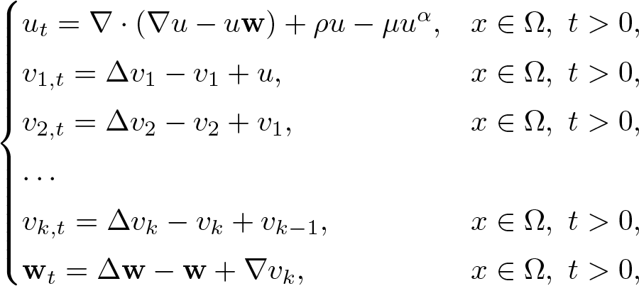
This article considers the system

(1.1)\begin{equation} \begin{cases} u_t = \nabla\cdot \left(\nabla u - u\bf{w} \right) + \rho u - \mu u^\alpha ,&x \in \Omega ,\ t \gt 0,\\ v_{1,t} = \Delta v_1 - v_1 + u,&x \in \Omega ,\ t \gt 0,\\ v_{2,t} = \Delta v_2 - v_2 + v_1,&x \in \Omega ,\ t \gt 0,\\ \ldots \\ v_{k,t} = \Delta v_k - v_k + v_{k - 1},&x \in \Omega ,\ t \gt 0,\\ {\bf{w}}_t = \Delta {\bf{w}} - {\bf{w}} + \nabla v_k,&x \in \Omega ,\ t \gt 0,\\ \dfrac{{\partial u}}{{\partial {\bf{n}}}} = \dfrac{{\partial {v_1}}}{{\partial {\bf{n}}}} = \cdots = \dfrac{{\partial {v_k}}}{{\partial {\bf{n}}}} = 0,\ {\mathbf{w}} = {\mathbf{0}},& x \in \partial \Omega ,\ t \gt 0,\\ \left( u_0,v_{i0},\bf{w}_0 \right)\left( x \right) = \left( u,v_i,\bf{w} \right)\left( x,0 \right),\ i = 1, \ldots ,k,&x \in \Omega , \end{cases}\end{equation}

where $\Omega \subset \mathbb{R}^n\left( {n \geqslant 1} \right)$ is a bounded domain with smooth boundary, $\bf{n}$ denotes the outward normal vector on $\partial \Omega $, the parameters ρ > 0, µ > 0, and α > 1. The functions $u\left( x,t \right)$ and $v_1\left( x,t \right)$ denote the organism density and the signal emitted by the organism itself respectively, $v_i\left(x,t\right)$ $(i=2,3,\ldots,k)$ represent the signal induced by the signal $v_{i-1}\left(x,t\right)$, the vector function ${\bf{w}}\left( x,t \right) = \left( w_1,w_2, \ldots ,w_n \right)\left( x,t \right)$ represents the velocity of u. The system (1.1) is a generalized version of the classical chemotaxis model (cf. [Reference Keller and Segel9, Reference Keller and Segel10]). For a broad overview over various types of chemotaxis processes, we refer the reader to the surveys [Reference Bellomo, Bellouquid, Tao and Winkler3, Reference Hillen and Painter5, Reference Horstmann6, Reference Lankeit and Winkler12, Reference Suzuki25, Reference Suzuki26] and the references therein.

\begin{equation*}f(u)=\rho u-\mu u^\alpha\end{equation*}

is the typical example of logistic source, where ρ > 0, µ > 0, and α > 1. Note that the analogous equations are used in the study of varies models. In biological phenomena, the reproduction or death of the population plays an important role in its life. Many mathematicians introduce the term to the chemotaxis model and obtain some related results. It is well known that an appropriate logistic damping can prevent blow-up of solutions to the classical Keller–Segel system

\begin{equation*} \begin{cases} u_t=\nabla\cdot(\nabla u-u\nabla v)+f(u),&x\in\Omega,\,t \gt 0,\\ v_t=\Delta v-v+u,&x\in\Omega,\,t \gt 0,\\ \nabla u\cdot\textbf{n}=\nabla v\cdot\textbf{n}=0,&x\in\partial\Omega,\,t \gt 0,\\ u(x,0)=u_0(x),v(x,0)=v_0(x),&x\in\Omega. \end{cases} \end{equation*}

Therefore, how far such favourable mathematical effect thereof can expand the solution theory when such logistic damping interacts with further and possibly destabilizing mechanisms is an interesting problem. The parabolic-elliptic Keller–Segel simplification (where v_t is replaced by 0) is considered in [Reference Tello and Winkler29] and it is shown that if α > 2, then the system possesses a unique and uniformly bounded global classical solution. In [Reference Winkler31], the existence of weak solutions is proved under more general conditions. For the parabolic-parabolic Keller–Segel system, in [Reference Winkler33], it is shown that if α = 2, µ > 0 is sufficiently large then the problem possesses a unique and uniformly bounded global-in-time classical solution. In [Reference Lankeit11], the global classical solution and large time behaviour are considered with α = 2. In [Reference Xiang40], Xiang shows the uniform-in-time boundedness for the corresponding 2D Neumann initial-boundary value problem in a large class of cell kinetics including sub-logistic sources. Global generalized solutions have been constructed in [Reference Viglialoro30] when $n\geqslant2$ and $\alpha \gt 2-\frac{1}{n}$. Then in [Reference Winkler38] and [Reference Yan and Fuest41] extension are obtained in the sense of weaker solution concept with the wider range $\alpha\geqslant\frac{2n+4}{n+4}$ and $\alpha \gt \min\{\frac{2n-2}{n},\frac{2n+4}{n+4}\}$. Recently, Winkler in [Reference Winkler39] showed that mild condition α > 1 on f, rules out the emergence of persistent Dirac-type singularities, known as a characteristic feature of unperturbed Keller–Segel systems corresponding to the choice $f\equiv0$. Besides, many authors are interested in qualitative convergence of the solution [Reference Winkler35–Reference Winkler37] and large time behaviour [Reference Cao4, Reference Winkler34] for such kind of models. Similar models can be seen in [Reference Lv and Wang15, Reference Lyu and Mao18–Reference Lyu and Wang20].

In the classical Chemotaxis system, the signal is produced by cells themselves directly. But in the real biological system, the production of the signal is substantially complicated. In [Reference Arditi, Tyutyunov, Morgulis, Govorukhin and Senina1, Reference Sapoukhina, Tyutyunov and Arditi24], the authors propose the acceleration assumption that the advective velocity variation (i.e. acceleration) rather than the velocity itself of the organism is supposed to be proportional to the gradient of the signal. Later, Mu and Tao in [Reference Mu and Tao21] introduce the acceleration assumption into chemotaxis models and consider the system (1.1) with k = 1, $\rho=\mu=0$ and the last equation is replaced by elliptic equation. It is proved that for reasonable initial data, the system with some boundary conditions admits global bounded solutions for $n\leqslant3$. For the fully parabolic case, Tao and Wang in [Reference Tao and Wang27] show that this new type of chemotaxis model with acceleration precludes the blow-up and admits globally bounded solutions in two and three dimensions. Besides, Mu, Tao, and Wang in [Reference Mu, Tao and Wang22] explore the qualitative behaviour of such prey-taxis systems with prey-induced acceleration and establish the global existence of classical solutions with uniform-in-time bounds in all spatial dimensions. Moreover, it is proved that the global stability of spatially homogeneous prey-only and coexistence steady states with decay rates under certain conditions on system parameters.

Motivated by the foregoing results, we proceed to consider a more intricate system denoted as (1.1). In this system, the acceleration is postulated to be directly proportional to the gradient of the signal, and the signal itself is generated by the organism via distinct processes. The principal objective of this article is to meticulously investigate the global dynamics of (1.1) within any dimensional space. Precisely, we will establish the existence of global classical solutions across all dimensions and probe into the global stability of constant steady states. Through this exploration, we can discern how the values of parameters influence and determine these dynamical characteristics of the solutions.

For the convenience of presentation, let

(1.2)\begin{equation} K_1=\begin{cases} \frac{2^{5-2\alpha}|\Omega|^{2-\alpha}}{1-2^{-(\alpha-1)}},&\text{if}\ \ \alpha \lt 2,\\ 1,&\text{if}\ \ \alpha\geqslant 2, \end{cases} \end{equation}

and K ₂ denotes the following Poincaré constant

(1.3)\begin{equation} K_2: = \left\{\mathop {\inf }\limits_{C \gt 0} C\left| {{{\left\| u -\overline{u}\right\|}_{{L^{\frac{2n}{n-2}}}\left( \Omega \right)}} \leqslant C{{\left\| {\nabla u} \right\|}_{{L^2}\left( \Omega \right)}}} \right.\ \text{for all}\ u \in {W^{1,2}}\left( \Omega \right) \right\}, \end{equation}

where

\begin{equation*}\overline{u}=\frac{1}{|\Omega|}\int_{\Omega}u.\end{equation*}

We suppose the initial data $\left( u_0,v_{10},v_{20},\ldots,v_{k0},\bf{w}_0 \right)$ satisfies

(1.4)\begin{equation} \begin{cases} u_0 \in C^0\ (\overline\Omega ),\ u_0 \geqslant 0,\ u_0\not \equiv 0,&in\ \Omega , \hfill \\ v_{i0} \in W^{1,\infty }(\Omega ),\ v_{i0} \geqslant 0,&in\ \Omega ,\ i=1,2,\ldots,k,\hfill \\ \mathbf{w}_0 \in W^{1,\infty }(\Omega ;\mathbb{R}^n),&in\ \Omega. \hfill \\ \end{cases} \end{equation}

The first principal result pertains to the global boundedness of solutions and is presented as follows.

Theorem 1.1. Let $\Omega\subset\mathbb{R}^n$ be a bounded domain with smooth boundary and let $k\in\mathbb{Z}^+$, ρ > 0. If one of the following conditions holds

\begin{equation*}\left( {{\bf{H1}}} \right):1\leqslant n \lt 2k + 2,\ \mu \gt 0,\ \alpha \gt 1,\end{equation*}

\begin{equation*}\left( {{\bf{H2}}} \right):2k + 2 \leqslant n \lt 4k + 2,\ \mu \gt 0,\ \alpha \gt \frac{{n + 2}}{{2k + 2}}\left( { \lt 2} \right),\end{equation*}

\begin{equation*}\left( {{\bf{H3}}} \right):n \geqslant 4k + 2,\ \text{either}\ \alpha \gt 2,\ \mu \gt 0\ \text{or}\ \alpha=2,\ \mu \gt \mu_0,\end{equation*}

where $\mu_0 \gt 0$ is a fixed constant. Then for any initial data satisfying condition (1.4), the system (1.1) possesses a unique classical solution $\left( u,v_1,v_2,\ldots,v_k,\bf{w} \right)$ satisfying

\begin{equation*}(u,v_1, \ldots ,v_k) \in {(C^0( \overline \Omega \times [0,+\infty)) \cap C^{2,1}( \overline\Omega\times (0,+\infty)))^{k + 1}},\end{equation*}

\begin{equation*}{\bf{w}} \in C^0( \overline \Omega\times [0,+\infty);\mathbb{R}^n)\cap C^{2,1}(\overline\Omega\times(0,+\infty);\mathbb{R}^n),\end{equation*}

and $u,v_i \gt 0$ in $\Omega\times\left(0,+\infty\right)$, where $i = 1,\ldots,k$. Moreover, the solution is uniformly bounded in time, i.e. there exists a constant C > 0 such that

\begin{equation*} \mathop {\sup }\limits_{t \in \left[ {0,+\infty } \right)} \left( {{{\left\| {u\left( {\cdot ,t} \right)} \right\|}_{{L^\infty }\left( \Omega \right)}} + \sum\limits_{i = 1}^k {{{\left\| {{v_i}\left( {\cdot ,t} \right)} \right\|}_{{W^{1,\infty }}\left( \Omega \right)}}} + {{\left\| {{\bf{w}}\left( {\cdot ,t} \right)} \right\|}_{{W^{1,\infty }}\left( \Omega \right)}}} \right)\leqslant C. \end{equation*}

Remark 1.1. The results presented in theorem 1.1 clearly suggest that the existence of the global classical solution of the system can be firmly established within a particular parameter range. Notably, this parameter range exhibits a characteristic of becoming more restricted or narrower as the spatial dimension experiences an increase. In fact, our detailed analysis reveals that when the conditions

\begin{equation*}n\geqslant6,\ \rho \gt 0,\ \text{either}\ \alpha \gt 2,\ \mu \gt 0\ \text{or}\ \alpha=2,\ \mu \gt \mu_0,\end{equation*}

are satisfied, which is significantly more relaxed in comparison to the conditions

\begin{equation*}n\geqslant4,\ \rho=\mu \gt 0,\ \alpha \gt \frac{1}{2}+\frac{n}{4}\end{equation*}

as proposed in [Reference Mu and Tao21], it can be deduced that the system admits the global classical solution, especially when k = 1. This finding not only broadens the understanding of the system’s behaviour but also offers a more comprehensive perspective on the relationship between the spatial dimension, the various parameters, and the existence of the global classical solution.

Our subsequent objective is to investigate the large-time behaviour of the solutions to (1.1). The system (1.1) possesses a non-trivial constant equilibrium, where

\begin{equation*} m:={\left( {\frac{\rho }{\mu }} \right)^{\frac{1}{{\alpha - 1}}}}. \end{equation*}

Subsequently, the global stability result is presented in the following theorem.

Theorem 1.2. Suppose the assumptions in theorem 1.1 hold. If

(1.5)\begin{equation} \mu \gt \begin{cases} \left(\frac{k}{8(k+1)}\right)^\frac{\alpha-1}{2}\rho^\frac{3-\alpha}{2},\quad&\text{if}\ \alpha\geqslant2,\\ \left(\frac{K_1K_2}{8}\right)^\frac{\alpha-1}{2}\rho^\frac{3-\alpha}{2},\quad&\text{if}\ 2-\frac{2}{n}\leqslant\alpha \lt 2, \end{cases} \end{equation}

then the solution $\left( {u,v_1, \ldots ,v_k,{\bf{w}}} \right)$ of the system (1.1) obtained in theorem 1.1 satisfies

\begin{equation*} {\left\| {u\left( {\cdot ,t} \right) - m} \right\|_{{W^{1,\infty }}\left( \Omega \right)}}+ \sum\limits_{i = 1}^k {{{\left\| {{v_i}\left( {\cdot ,t} \right)-m} \right\|}_{{W^{1,\infty }}\left( \Omega \right)}}} + {\left\| {{\bf{w}}\left( {\cdot ,t} \right)} \right\|_{{W^{1,\infty }}\left( \Omega \right)}} \to 0\quad \text{as}\ t \to \infty. \end{equation*}

Moreover, if

(1.6)\begin{equation} \mu \gt \begin{cases} \left(\frac{k}{8(k+1)}\right)^\frac{\alpha-1}{2}\rho^\frac{3-\alpha}{2},\quad&\text{if}\ \alpha\geqslant2,\\ \max\left\{\left(\frac{k}{8(k+1)K_1}\right)^\frac{\alpha-1}{2},\left(\frac{K_1K_2}{8}\right)^\frac{\alpha-1}{2}\right\}\rho^\frac{3-\alpha}{2},\quad&\text{if}\ 2-\frac{2}{n}\leqslant\alpha \lt 2, \end{cases} \end{equation}

then there exist some constants $C,\tau \gt 0$ such that

\begin{align*}&{\left\| {u\left( {\cdot ,t} \right) - m} \right\|_{{W^{1,\infty }}\left( \Omega \right)}}+ \sum\limits_{i = 1}^k {{{\left\| {{v_i}\left( {\cdot ,t} \right)-m} \right\|}_{{W^{1,\infty }}\left( \Omega \right)}}} + {\left\| {{\bf{w}}\left( {\cdot ,t} \right)} \right\|_{{W^{1,\infty }}\left( \Omega \right)}}\\ & \quad \leqslant Ce^{-\tau t}\quad \text{for all}\ t \gt 0.\end{align*}

Main ideas. For the existence of global classical solutions of (1.1), we initially establish a criterion which can help us to draw the conclusion. Specifically, if either

\begin{equation*}\left\| {u\left( {\cdot ,t} \right)} \right\|_{{L^{{p_1}}}\left( \Omega \right)}\quad\text{for some }p_1 \gt \frac{n}{2k+2}\end{equation*}

or

\begin{equation*}\int_t^{t + \tau } {\left\| {u\left( {\cdot ,s} \right)} \right\|_{{L^{{p_2}}}\left( \Omega \right)}^{{p_2}}ds}\quad\text{for some }p_2 \gt \frac{n+2}{2k+2}\end{equation*}

is bounded, then (1.1) admits the global classical solution. Subsequently, we do some estimates for three cases, namely

\begin{equation*}n \lt 2k+2,\ 2k+2\leqslant n \lt 4k+2\ \text{and}\ n\geqslant4k+2\end{equation*}

in order to satisfy one of the criteria respectively. When $n \lt 2k+2$, it is evident that $\|u(\cdot,t)\|_{L^1(\Omega)}$ is bounded. For the case $2k+2\leqslant n \lt 4k+2$, we limit the range of α to attain the boundedness of $\int_t^{t + \tau } {\left\| {u\left( {\cdot ,s} \right)} \right\|_{{L^\alpha}\left( \Omega \right)}^{\alpha}ds}$. In the situation where $n\geqslant4k+2$, the Young inequality and the maximal Sobolev regularity for the linear heat equations assist us in obtaining the boundedness of $\|u(\cdot,t)\|_{L^p(\Omega)}$.

To determine the convergence rate of solutions for the system involving subquadratic degradation, our crucial approach is to employ a remarkable inequality [Reference Winkler37, Lemma 3.4], namely lemma 2.4. By analysing the energy functional

\begin{equation*} \int_\Omega {{\left( {u - m - m\ln \frac{u}{m}} \right)}} +A\sum\limits_{i = 1}^k {\int_\Omega\left(v_i-\overline{v_i}\right)^2} +B\int_\Omega {{{\left| {\bf{w}} \right|}^2}}, \end{equation*}

where A and B are certain constants, we deduce that the quantity

\begin{equation*}\int_{T}^{+\infty}\left\|u-m\right\|_{L^{\frac{2}{3-\alpha}}(\Omega)}^{2}ds\end{equation*}

is finite, which indicates the stability of u. Subsequently, the stability of v_i and w can be acquired. To analyse the convergence rate, we need to consider the standard energy functional

\begin{equation*} \int_\Omega {{\left( {u - m - m\ln \frac{u}{m}} \right)}} +A\sum\limits_{i = 1}^k {\int_\Omega {{{\left( {{v_i} - m} \right)}^2}} } +B\int_\Omega {{{\left| {\bf{w}} \right|}^2}}, \end{equation*}

which, in conjunction with the aforementioned remarkable inequality [Reference Winkler37, Lemma 3.4], implies the exponential convergence of u, v_i, and w. For the superquadratic or quadratic degradation, the method is conventional. Through analysing the energy functional

\begin{equation*}\int_\Omega {{\left( {u - m - m\ln \frac{u}{m}} \right)}} +A\sum\limits_{i = 1}^k {\int_\Omega {{{\left( {{v_i} - m} \right)}^2}} } +B\int_\Omega {{{\left| {\bf{w}} \right|}^2}},\end{equation*}

the conclusion can be readily derived. It should be noted that due to the large number of equations, it is essential to ascertain the positive definiteness of the tridiagonal matrix during the proof process.

Plan of the article. This article is organized in the following manner. Section 2 is dedicated to presenting certain facts that are crucial in establishing the global existence of solutions. In §3, we elaborate on the local existence and extensibility of solutions to the system and subsequently derive two criteria for the global boundedness of solutions. Thereafter, we deduce some a priori estimates to fulfil the criterion and thereby obtain the global bounded solutions of (1.1). Finally, in §4, by constructing suitable Lyapunov functionals, the global convergence to the constant steady states as stated in theorem 1.2 is demonstrated.

2. Preliminaries

We recall some elementary estimates of solutions to the linear heat equation.

Lemma 2.1. Let $T\in \left( {0, + \infty } \right],$ $q \geqslant 1.$ For each

\begin{equation*} r_1 \in \begin{cases} [ 1,\frac{nq}{n -2q}),&q \leqslant \frac{n}{2},\\ [ 1,+\infty ],&q \gt \frac{n}{2}, \end{cases} \end{equation*}

\begin{equation*} r_2 \in \begin{cases} [ 1,\frac{nq}{n +2- 2q} ),&q \leqslant \frac{n + 2}{2},\\ [ 1,+\infty ],&q \gt \frac{n + 2}{2}, \end{cases} \end{equation*}

and

\begin{equation*} r_3 \in \begin{cases} [ 1,\frac{nq}{n -q} ),&q \leqslant n,\\ [ 1,+\infty ],&q \gt n, \end{cases} \end{equation*}

there exist some constants $C_i \gt 0\ (i=1,2,3)$ which are independent of T and τ with the property that if $z_0 \in W^{1,\infty }\left( \Omega \right)$ and if

\begin{equation*}z \in C^0( {\overline \Omega \times [ 0,T)} ) \cap C^{2,1}( \overline \Omega \times ( 0,T) ),\quad u\in C^0( {\overline \Omega \times [ 0,T)} )\end{equation*}

fulfil

\begin{equation*} \begin{cases} z_t = \Delta z - z + u,&x \in \Omega ,\ t \in \left(0,T\right),\\ \dfrac{\partial z}{\partial\bf{n}} = 0\ \text{or }z=0,&x \in \partial \Omega ,\ t \in \left(0,T\right),\\ z\left( x,0 \right) = z_0\left( x \right),&x \in \Omega, \end{cases} \end{equation*}

then

(2.1)\begin{equation} {\left\| z\left( \cdot ,t \right) \right\|_{L^{r_1}\left( \Omega \right)}} \leqslant C_1\left( {{{\left\| z_0 \right\|}_{{W^{1,\infty }}\left( \Omega \right)}} + \mathop {\sup }\limits_{s \in \left( 0,T\right)} {{\left\| {u\left( \cdot ,s \right)} \right\|}_{L^q\left( \Omega \right)}}} \right)\quad \text{for all}\ t \in \left( 0,T\right), \end{equation}

(2.2)\begin{equation} {\left\| {z\left( {\cdot ,t} \right)} \right\|_{{L^{{r_2}}}\left( \Omega \right)}} \leqslant C_2\left( {{{\left\| {{z_0}} \right\|}_{{W^{1,\infty }}\left( \Omega \right)}} + \int_t^{t + \tau } {\left\| {u\left( {\cdot ,s} \right)} \right\|_{{L^q}\left( \Omega \right)}^q ds} } \right)\quad {\text{for all}}\;t \in \left( {0,T-\tau } \right), \end{equation}

and

(2.3)\begin{equation} {\left\| {\nabla z\left( \cdot ,t \right)} \right\|_{L^{r_3}\left( \Omega \right)}} \leqslant C_3\left( {{{\left\| z_0 \right\|}_{{W^{1,\infty }}\left( \Omega \right)}} + \mathop {\sup }\limits_{s \in \left( 0,T\right)} {{\left\| {u\left( \cdot ,s \right)} \right\|}_{L^q\left( \Omega \right)}}} \right)\quad\text{for all}\ t \in \left( 0,T\right), \end{equation}

where $0 \lt \tau \lt T$.

Proof. Case I: Neumann boundary condition. The proof of (2.2) can be found in [Reference Lyu17, Lemma 2.2] and the proof of (2.3) can be found in [Reference Horstmann and Winkler7, Lemma 4.1], so we only prove (2.1) below. The variation-of-constants formula for z yields

\begin{equation*} z=e^{t(\Delta-1)}z_0+\int_0^te^{(t-s)(\Delta-1)}u(s)ds\quad\text{for all}\ t\in(0,T), \end{equation*}

which, along with the smoothing property of the Neumann Laplace semigroup [Reference Winkler32] and Hölder’s inequality, gives that with $\lambda,C_1 \gt 0$,

\begin{align*} \begin{aligned} \|z(\cdot,t)\|_{L^{r_1}(\Omega)}\leqslant& C_1\|z_0\|_{L^\infty(\Omega)}+\int_0^t \| e^{(t-s)\Delta}u(s)\|_{L^{r_1}(\Omega)}ds\\ \leqslant& C_1\|z_0\|_{L^\infty(\Omega)}+C_1\int_0^te^{-\lambda(t-s)}\left(1+(t-s)^{-\frac{n}{2}\left(\frac{1}{q}-\frac{1}{r_1}\right)_+}\right)\|u(s)\|_{L^q(\Omega)}ds\\ \leqslant& C_1\|z_0\|_{L^\infty(\Omega)}+C_1\mathop {\sup }\limits_{s\in\left(0,T\right)}\left\|u\left(\cdot,s\right) \right\|_{L^q\left(\Omega \right)}\int_0^te^{-\lambda(t-s)}\\ & \quad \times \left(1+(t-s)^{-\frac{n}{2}\left(\frac{1}{q}-\frac{1}{r_1}\right)_+}\right)ds \end{aligned} \end{align*}

for all $t\in(0,T)$. If $q\leqslant \frac{n}{2}$, then

(2.4)\begin{equation} \begin{aligned} &-\frac{n}{2}\left(\frac{1}{q}-\frac{1}{r_1}\right)_+\\ \gt &-\frac{n}{2}\left(\frac{1}{q}-\frac{n-2q}{nq}\right)\\ =&-1. \end{aligned} \end{equation}

If $q \gt \frac{n}{2}$, then

(2.5)\begin{equation} \begin{aligned} &-\frac{n}{2}\left(\frac{1}{q}-\frac{1}{r_1}\right)_+\\ \geqslant&-\frac{n}{2q}\\ \gt &-1. \end{aligned} \end{equation}

Combining (2.4) and (2.5), we obtain that there exists $C_2 \gt 0$ such that

\begin{equation*}\int_0^te^{-\lambda(t-s)}\left(1+(t-s)^{-\frac{n}{2}\left(\frac{1}{q}-\frac{1}{r_1}\right)_+}\right)ds\leqslant C_2\quad\text{for all}\ t\in(0,T).\end{equation*}

Therefore, (2.1) can be derived easily.

Case II: Dirichlet boundary condition. The proof of the results is similar to the case of Neumann boundary condition, with the sole caveat that we must pay attention to utilizing the properties of Dirichlet semigroups [Reference Mu, Tao and Wang22, Lemma 2.4] in the proof.

The following is the maximal Sobolev regularity for the linear heat equations [Reference Ishida, Seki and Yokota8, Lemma 2.1].

Lemma 2.2. Let $r \in(n,+\infty)$. We can find a constant $M_r \gt 0$ with the property that whenever $T\in(0,+\infty]$, $\tau _0\in \left[0,T\right)$,

\begin{equation*}z\in C^0(\overline{\Omega}\times[0,T))\cap C^{2,1}(\overline{\Omega}\times(0,T)),\quad w\in C^0(\overline{\Omega}\times[0,T)) \end{equation*}

satisfy

\begin{equation*} \begin{cases} z_t=\Delta z-z+w, &x\in\Omega,\,t\in(0,T),\\ \displaystyle\frac{\partial z}{\partial\bf{n}}=0\ \text{or }z=0, &x\in\partial\Omega,t\in(0,T),\\ z(x,0)=z_0(x), &x\in\Omega \end{cases} \end{equation*}

and $z\left(\cdot,\ \tau_0\right)\in {W^{2,r}}\left(\Omega\right)$ with $\dfrac{{\partial z\left( {\cdot ,{\tau _0}} \right)}}{{\partial\bf{n}}} = 0$, then we have

\begin{equation*} \int_{{\tau _0}}^T {\int_\Omega {{e^{r\tau }}\left( {{{\left| z \right|}^r} + {{\left| {\nabla z} \right|}^r} + {{\left| {{z_t}} \right|}^r}} \right)} } d\tau \leqslant M_r\int_{{\tau _0}}^T {e^{r\tau }\left\|w\right\|_{{L^r}\left(\Omega\right)}^r}d\tau+M_r\left\| {z\left( {\cdot ,{\tau _0}} \right)} \right\|_{{W^{2,r}}\left( \Omega \right)}^r. \end{equation*}

Now, an inequality [Reference Lyu and Wang19, Lemma 2.1] is stated as follows.

Lemma 2.3. Let a > 0, b > 0, and $q\geqslant1$. We have

\begin{align*} \left(a-b\right)\left(a^q-b^q\right)\geqslant b^{q-1}\left(a-b\right)^2. \end{align*}

The last, we shall recall an important inequality [Reference Winkler37, Lemma 3.4] below.

Lemma 2.4. Let σ > 1. Then

\begin{equation*} \left(\xi^{\sigma-1}-1\right)(\xi-1) \geqslant K(\xi-1)^2 \quad \text {for all } \xi \in[0,2], \end{equation*}

where

\begin{equation*} K:= \begin{cases}(\sigma-1)2^{\sigma-2} & \text {if } \sigma \in(1,2), \\ 1 & \text {if } \sigma \in[2,+\infty) .\end{cases} \end{equation*}

3. Global existence and uniform boundedness

In this section, our goal is to study the global existence and boundedness of solutions to the system (1.1).

3.1. Local existence and extensibility criterion

Using a fixed point theorem, we can establish the local existence of solutions to the system. For the sake of brevity, we will not go into the specifics of the proof here. Details can be seen in [Reference Mu and Tao21, Reference Mu, Tao and Wang22].

Lemma 3.1. Suppose that the conditions in theorem 1.1 hold. Then there exists $T_{\max} \in \left( {0,+\infty } \right]$ such that the system (1.1) has a unique classical solution $\left( {u,v_1, \ldots ,v_k,{\bf{w}}} \right)$ satisfying

\begin{equation*}u,v_1, \ldots ,v_k\in C^0(\overline\Omega \times [0,T_{\max })) \cap C^{2,1}(\overline\Omega \times (0,T_{\max })),\end{equation*}

\begin{equation*}{\bf{w}} \in C^0(\overline\Omega \times [0,T_{\max });\mathbb{R}^n) \cap C^{2,1}(\overline\Omega \times (0,T_{\max });\mathbb{R}^n),\end{equation*}

and $u,v_i \gt 0$ in $\overline\Omega \times \left(0,T_{\max}\right)$, where $i = 1,\ldots,k.$ Moreover, if $T_{\max} \lt +\infty$, then

\begin{equation*}\lim\limits_{t\nearrow T_{\max}}\left(\left\|u\left(\cdot,t\right)\right\|_{L^\infty(\Omega)}+\sum_{i=1}^k\left\|v_i\left(\cdot,t\right) \right\|_{W^{1,\infty}(\Omega)}+\|\textbf{w}\|_{W^{1,\infty}(\Omega)}\right)=+\infty .\end{equation*}

3.2. Estimates for u

Now, some basic estimates for u can be obtained below.

Lemma 3.2. If µ > 0 and ρ > 0, then

(3.1)\begin{equation} {\left\| {u\left( \cdot ,t \right)} \right\|_{L^1\left( \Omega \right)}} \leqslant \max \left\{{{{\left\| u_0\right\|}_{{L^1}\left( \Omega \right)}},{\left( {\frac{\rho }{\mu }} \right)^{\frac{1}{{\alpha - 1}}}}\left| \Omega \right|} \right\}\quad {\text{for all}}\;t \in \left( {0,T_{\max }} \right) \end{equation}

and there exists a constant C > 0 such that

(3.2)\begin{equation} \int_t^{t + \tau } {\int_\Omega {u^\alpha } } \leqslant C\quad \text{for all}\ t \in \left( 0,T_{\max } - \tau \right), \end{equation}

where $\tau: = \min \left\{1,\frac{T_{\max }}{2} \right\}.$

Proof. Integrating the first equation of (1.1) over Ω and integrating by parts, we find

(3.3)\begin{equation} \frac{d}{{dt}}\int_\Omega u = \rho \int_\Omega u - \mu \int_\Omega {u^\alpha } \quad \text{for all}\ t \in \left( 0,T_{\max } \right). \end{equation}

If µ > 0 and ρ > 0, then due to α > 1 and Hölder’s inequality, we conclude

\begin{equation*}{\left\| u \right\|_{{L^1}\left( \Omega \right)}} \leqslant {\left| \Omega \right|^{1 - \frac{1}{\alpha }}}{\left\| u \right\|_{{L^\alpha }\left( \Omega \right)}}\quad \text{for all}\ t \in \left( 0,T_{\max } \right),\end{equation*}

which, along with (3.3), implies that

\begin{equation*}\frac{d}{{dt}}{\left\| u \right\|_{{L^1}\left( \Omega \right)}} \leqslant \rho{\left\| u \right\|_{{L^1}\left( \Omega \right)}} - \frac{\mu }{{{{\left| \Omega \right|}^{\alpha - 1}}}}\left\| u \right\|_{{L^1}\left( \Omega \right)}^\alpha\quad \text{for all}\ t \in \left( 0,T_{\max } \right) .\end{equation*}

Solving this ordinary differential inequality and noticing the positivity of u, we get (3.1). Integrating (3.3) over $\left( {t,t + \tau } \right)$ and using (3.1), we derive (3.2).

The following is a basic inequality on u, which is useful for the L^p-estimate of u.

Lemma 3.3. For all p > 1 and ɛ > 0, we find

\begin{equation*}\begin{aligned} &\int_\Omega {{u^p}} \leqslant {e^{- \left( {p + 1} \right)\left( {t - {\tau _0}} \right)}}\int_\Omega {{u^p}\left( {{\tau _0}} \right)} \\ &\quad + \int_{{\tau _0}}^t {{e^{- \left( {p + 1} \right)\left( {t - \tau } \right)}}\left[ {\left( {\rho p + p + 1} \right)\int_\Omega u^p(\tau)} \right.} \\ &\quad + \left. {\left(p\varepsilon +\frac{M_{p+1}^{k+1}}{\varepsilon^p} \right)\frac{{p - 1}}{{p + 1}}\int_\Omega u^{p + 1}(\tau) -\mu p\int_\Omega {{u^{p + \alpha - 1}(\tau)}} } \right]d\tau\\ &\quad + \frac{{p - 1}}{(p+1)\varepsilon^p}\left[ {M_{p + 1}}\left\| {{\bf{w}}\left( {\cdot ,{\tau _0}} \right)} \right\|_{{W^{2,p + 1}}\left( \Omega \right)}^{p + 1} +M_{p + 1}^2\left\| {{v_k}\left( {\cdot ,{\tau _0}} \right)} \right\|_{{W^{2,p + 1}}\left( \Omega \right)}^{p + 1} \right. \\ &\quad \left. + \cdots + M_{p + 1}^{{{k + 1}}}\left\| {{v_1}\left( {\cdot ,{\tau _0}} \right)} \right\|_{{W^{2,p + 1}}\left( \Omega \right)}^{p + 1} \right] \end{aligned} \end{equation*}

for any $\tau_0\in\left(0,T_{\max}\right)$ and $t\in\left(\tau_0,T_{\max}\right)$, where $M_{p+1}$ is a constant which is defined in lemma 2.2.

Proof. Utilizing the first equation of (1.1), the boundary conditions and integration by parts, we get

(3.4)\begin{equation} \begin{aligned} \frac{d}{{dt}}\int_\Omega {{u^p}} &= p\int_\Omega {{u^{p - 1}}{u_t}} = p\int_\Omega {{u^{p - 1}}\left( {\nabla \cdot \left( {\nabla u - u{\bf{w}}} \right) + \rho u - \mu {u^\alpha}} \right)} \\ &= - p\left( {p - 1} \right)\int_\Omega {{u^{p - 2}}{{\left| {\nabla u} \right|}^2}} + p\left( {p - 1} \right)\int_\Omega {{u^{p - 1}}{\bf{w}} \cdot \nabla u}\\ &\quad\quad + \rho p\int_\Omega u^p- \mu p\int_\Omega u^{p+\alpha-1}\\ &\leqslant \left( {p - 1} \right)\int_\Omega {{\bf{w}} \cdot \nabla {u^p}} + \rho p\int_\Omega u^p- \mu p\int_\Omega u^{p+\alpha-1}\\ &= - \left( {p - 1} \right)\int_\Omega\left(\nabla \cdot{\bf{w}}\right) {u^p}+ \rho p\int_\Omega u^p- \mu p\int_\Omega u^{p+\alpha-1}\\ &\leqslant \frac{p\left(p-1\right)}{p+1}\varepsilon\int_\Omega u^{p+1} + \frac{p-1}{(p+1)\varepsilon^p}\int_\Omega \left|\nabla\cdot\bf{w}\right|^{p + 1}\\ &\quad\quad + \rho p\int_\Omega u^p- \mu p\int_\Omega u^{p+\alpha-1}\quad\text{for any } t\in\left(0,T_{\max}\right). \end{aligned} \end{equation}

Adding $\left( {p + 1} \right)\int_\Omega {{u^p}} $ to both sides of (3.4), we obtain

\begin{align*} &\frac{d}{dt}\int_\Omega {u^p}+\left(p+1\right)\int_\Omega {u^p} \\ \leqslant&\left(\rho p+p+1\right)\int_\Omega u^p+\frac{p\left(p-1\right)}{p+1}\varepsilon\int_\Omega u^{p+1}-\mu p \int_\Omega u^{p+\alpha-1}+\frac{p-1}{(p+1)\varepsilon^p}\int_\Omega\left|\nabla\cdot\bf{w}\right|^{p+1} \end{align*}

for any $t\in\left(0,T_{\max}\right)$ which yields

(3.5)\begin{equation} \begin{aligned} \int_\Omega {{u^p}} &\leqslant {e^{- \left( {p + 1} \right)\left( {t - {\tau _0}} \right)}}\int_\Omega {{u^p}\left( {{\tau _0}} \right)} + \int_{{\tau _0}}^t {{e^{- \left( {p + 1} \right)\left( {t - \tau } \right)}}\left[ {\left( {\rho p + p + 1} \right)\int_\Omega u^p(\tau)} \right.}+\frac{{p\left( {p - 1} \right)}}{{p + 1}}\varepsilon \\ &\left.\int_\Omega u^{p+1}(\tau) - \mu p \int_\Omega u^{p+\alpha-1}(\tau) +\frac{p-1}{(p+1)\varepsilon^p}\int_\Omega\left|\nabla\cdot\bf{w}(\tau)\right|^{p+1}\right]d\tau\quad\text{for any } t\in\left(0,T_{\max}\right). \end{aligned} \end{equation}

By lemma 2.2, we find

\begin{equation*} \begin{aligned} &\int_{{\tau_0}}^t {{e^{- \left( {p + 1} \right)\left(t-\tau\right)}}} \int_\Omega {{{\left| {\nabla\cdot{\bf{w}}} \right|}^{p + 1}}}\\ \leqslant &{M_{p + 1}}\left\| {{\bf{w}}\left( {\cdot ,{\tau _0}} \right)} \right\|_{{W^{2,p + 1}}\left( \Omega \right)}^{p + 1} + {M_{p + 1}}\int_{{\tau _0}}^t {{e^{- \left( {p + 1} \right)\left( {t - {\tau}} \right)}}} \int_\Omega {{{\left| {\nabla {v_k}(\tau)} \right|}^{p + 1}}}d\tau\\ \leqslant &{M_{p + 1}}\left\| {{\bf{w}}\left( {\cdot ,{\tau _0}} \right)} \right\|_{{W^{2,p + 1}}\left( \Omega \right)}^{p + 1} + M_{p + 1}^2\left\| {{v_k}\left( {\cdot ,{\tau _0}} \right)} \right\|_{{W^{2,p + 1}}\left( \Omega \right)}^{p + 1} + M_{p + 1}^2\int_{{\tau _0}}^t {{e^{- \left( {p + 1} \right)\left( {t - {\tau}} \right)}}}\\ & \int_\Omega {{{\left| {{v_{k - 1}(\tau)}} \right|}^{p + 1}}}d\tau\\ \leqslant &{M_{p + 1}}\left\| {{\bf{w}}\left( {\cdot ,{\tau _0}} \right)} \right\|_{{W^{2,p + 1}}\left( \Omega \right)}^{p + 1} + M_{p + 1}^2\left\| {{v_k}\left( {\cdot ,{\tau _0}} \right)} \right\|_{{W^{2,p + 1}}\left( \Omega \right)}^{p + 1} + \cdots+ M_{p + 1}^{{{k + 1}}}\left\| {{v_1}\left( {\cdot ,{\tau _0}} \right)} \right\|_{{W^{2,p + 1}}\left( \Omega \right)}^{p + 1} \\ & + M_{p + 1}^{{{k + 1}}}\int_{{\tau _0}}^t {{e^{- \left( {p + 1} \right)\left( {t - {\tau}} \right)}}} \int_\Omega {{u^{p + 1}(\tau)}}d\tau\quad\text{for any }\tau_0\in\left(0,T_{\max}\right) \text{and } t\in\left(\tau_0,T_{\max}\right) \end{aligned} \end{equation*}

which, along with (3.5), implies the desired result.

Now, the L^p-estimate of u can be obtained when α > 2.

Lemma 3.4. Let α > 2 and µ > 0. For any p > 1, there exists a constant $C=C\left(p\right) \gt 0$ such that

\begin{equation*}\int_\Omega u^p\leqslant C\quad\text{for any }t\in\left(0,T_{\max}\right).\end{equation*}

Proof. According to lemma 3.3, it holds that with ɛ = 1,

(3.6)\begin{equation} \begin{aligned} &\quad\int_\Omega {{u^p}} \leqslant {e^{- \left( {p + 1} \right)\left( {t - {\tau _0}} \right)}}\int_\Omega {{u^p}\left( {{\tau _0}} \right)} \\ &+ \int_{{\tau _0}}^t {{e^{- \left( {p + 1} \right)\left( {t - \tau } \right)}}\left[ {\left( {\rho p + p + 1} \right)\int_\Omega {{u^p}}(\tau) } \right.} + \left(p+M_{p+1}^{k+1}\right) \\ & \left. \times \frac{{p - 1}}{{p + 1}}\int_\Omega u^{p+1}(\tau) - \mu p \int_\Omega {{u^{p + \alpha - 1}}}(\tau) \right]d\tau\\ &+ \frac{{p - 1}}{(p+1)}\left[ {M_{p + 1}}\left\| {{\bf{w}}\left( {\cdot ,{\tau _0}} \right)} \right\|_{{W^{2,p + 1}}\left( \Omega \right)}^{p + 1} + M_{p + 1}^2\left\| {{v_k}\left( {\cdot ,{\tau _0}} \right)} \right\|_{{W^{2,p + 1}}\left( \Omega \right)}^{p + 1}\right. \\ & \left. \times + \cdots + M_{p + 1}^{{{k + 1}}}\left\| {{v_1}\left( {\cdot ,{\tau _0}} \right)} \right\|_{{W^{2,p + 1}}\left( \Omega \right)}^{p + 1} \right] \end{aligned} \end{equation}

for any $\tau_0\in\left(0,T_{\max}\right)$ and $t\in\left(\tau_0,T_{\max}\right)$. Noticing Young’s inequality, we find a constant $C_1 \gt 0$ such that

\begin{equation*} \left(\rho p+p+1\right)\int_\Omega {{u^p}} \leqslant\frac{\mu p}{2}\int_\Omega u^{p+\alpha-1}+ C_1\quad\text{for any }t\in\left(0,T_{\max}\right) \end{equation*}

and

\begin{equation*} \left(p+M_{p+1}^{k+1}\right)\frac{p-1}{p+1}\int_\Omega u^{p + 1}\leqslant\frac{\mu p}{2}\int_\Omega u^{p+\alpha-1}+C_1\quad\text{for any }t\in\left(0,T_{\max}\right). \end{equation*}

Inserting them into (3.6), we find a constant C > 0 such that $\int_\Omega {{u^p}} \leqslant C.$ Then the lemma is proved.

When α = 2, the L^p-estimate of u is derived under the condition that µ > 0 is sufficiently large.

Lemma 3.5. Let α = 2 and $p_0 \gt \frac{n }{2k + 2}$. If

\begin{equation*}\mu \gt \frac{p_0-1}{p_0}M_{p_0+1}^{\frac{k+1}{p_0+1}},\end{equation*}

then there exists a constant $C=C(p_0) \gt 0$ such that

\begin{equation*}\int_\Omega u^{p_0}dx\leqslant C\quad\text{for any }t \in \left(0,T_{\max}\right).\end{equation*}

Proof. Let

\begin{equation*}g(\varepsilon)=\left(\varepsilon +\frac{M_{p_0+1}^{k+1}}{p_0\varepsilon^{p_0}}\right)\frac{p_0-1}{p_0+1},\quad \varepsilon\in(0,+\infty),\end{equation*}

then

\begin{equation*}g'(\varepsilon)=\left(1- \frac{M_{p_0+1}^{k+1}}{\varepsilon^{p_0+1}}\right)\frac{p_0-1}{p_0+1}=0\end{equation*}

yields $g(\varepsilon)$ attains its minimum value

\begin{equation*}\frac{p_0-1}{p_0}M_{p_0+1}^{\frac{k+1}{p_0+1}}\end{equation*}

at $\varepsilon=M_{p_0+1}^{\frac{k+1}{p_0+1}}$. Due to

\begin{equation*}\mu \gt \frac{p_0-1}{p_0}M_{p_0+1}^{\frac{k+1}{p_0+1}}\end{equation*}

and the continuity of the function $g(\varepsilon)$, there exists a constant $\varepsilon_0 \gt 0$ such that

(3.7)\begin{equation} \mu \gt g(\varepsilon_0)\geqslant\frac{p_0-1}{p_0}M_{p_0+1}^{\frac{k+1}{p_0+1}}. \end{equation}

By lemma 3.3, we obtain with $p=p_0$ and $\varepsilon=\varepsilon_0$,

\begin{equation*}\begin{aligned} &\quad\int_\Omega u^{p_0}\leqslant e^{-\left(p_0+1\right)\left(t-\tau_0 \right)}\int_\Omega u^{p_0}\left(\tau_0\right)\\ &+\int_{\tau_0}^t e^{-\left(p_0+1\right)\left(t-\tau\right)}\left\{\left(\rho p_0+p_0+1\right)\int_\Omega u^{p_0}(\tau)\right. \\ &\left. -p_0\left[\mu-\left(\varepsilon_0 +\frac{M_{p_0+1}^{k+1}}{p_0\varepsilon_0^{p_0}}\right)\frac{p_0-1}{p_0+1}\right]\int_\Omega u^{p_0+1}(\tau)\right\}d\tau \\ & +\frac{p_0-1}{(p_0+1)\varepsilon_0^{p_0}}\left[M_{p_0+1}\left\|\bf{w}\left(\cdot ,\tau_0\right)\right\|_{W^{2,p_0+1}\left(\Omega\right)}^{p_0+1}+M_{p_0+1}^2\left\|v_k\left( \cdot,\tau_0\right)\right\|_{W^{2,p_0+1}\left(\Omega\right)}^{p_0+1}\right. \\ &\left. +\cdots+M_{p_0 +1}^{k+1}\left\|v_1\left(\cdot,\tau _0\right)\right\|_{W^{2,p_0+1}\left(\Omega \right)}^{p_0+1}\right] \end{aligned} \end{equation*}

for any $\tau_0\in\left(0,T_{\max}\right)$ and $t\in\left(\tau_0,T_{\max}\right)$, which along with (3.7), Young’s inequality,

\begin{equation*}\left(\rho p_0+p_0+1\right)\int_\Omega u^{p_0}(\tau)\leqslant\frac12p_0\left[\mu-\left(\varepsilon_0+\frac{M_{p_0+1}^{k+1}}{p_0\varepsilon_0^{p_0}}\right)\frac{p_0-1}{p_0+1}\right]\int_\Omega u^{p_0+1}(\tau)+C_1\end{equation*}

with a constant $C_1 \gt 0$ and lemma 3.1, implies the desired result.

3.3. Two refined criteria of global existence

We are in a position to derive the following boundedness criterions.

Lemma 3.6. Suppose that µ > 0 and ρ > 0. If for some

\begin{equation*}{p_1} \gt \frac{n}{2k+2},\end{equation*}

there exists M > 0 such that

(3.8)\begin{equation} \left\| {u\left( {\cdot ,t} \right)} \right\|_{{L^{{p_1}}}\left( \Omega \right)} \leqslant M\quad \text{for all}\ t \in \left({0,{T_{\max }}} \right), \end{equation}

or for some

\begin{equation*}{p_2} \gt \frac{n+2}{2k+2},\end{equation*}

there exists M > 0 such that

(3.9)\begin{equation} \int_t^{t + \tau } {\left\| {u\left( {\cdot ,s} \right)} \right\|_{{L^{{p_2}}}\left( \Omega \right)}^{{p_2}}ds} \leqslant M\quad \text{for all}\ t \in \left({0,T_{\max }-\tau} \right), \end{equation}

then there exists a constant C > 0 such that

(3.10)\begin{equation} {\left\| {u\left( {\cdot ,t} \right)} \right\|_{{L^\infty }\left( \Omega \right)}} + \sum\limits_{i = 1}^k {{{\left\| {{v_i}\left( {\cdot ,t} \right)} \right\|}_{{W^{1,\infty }}\left( \Omega \right)}}} + {\left\| {{\bf{w}}\left( {\cdot ,t} \right)} \right\|_{{W^{1,\infty }}\left( \Omega \right)}} \leqslant C\quad\text{for all}\ t \in \left( 0,T_{\max } \right). \end{equation}

Proof. Step 1: We claim that there exist $p_0 \gt n$ and $C_1 \gt 0$ such that

\begin{equation*} \mathop {\sup }\limits_{t \in \left( 0,T_{\max } \right)} {\left\| {{\bf{w}}\left( \cdot ,t \right)} \right\|_{L^{p_0}(\Omega)}} \leqslant C_1. \end{equation*}

Case of (3.8). From lemma 3.2 and (2.1) of lemma 2.1, we have that for any $\sigma_1\in\left[1,\left(\frac{np_1}{n-2p_1}\right)_+\right)$, there exist two constants $C_2 \gt 0$ and $C_3 \gt 0$ such that

\begin{align*} &{\left\| {v_1\left( \cdot ,t \right)} \right\|_{L^{\sigma_1}\left( \Omega \right)}} \leqslant C_2\left( {{{\left\| v_{1,0} \right\|}_{W^{1,\infty }\left( \Omega \right)}} + \mathop {\sup }\limits_{s \in \left( 0,T_{\max} \right)} {{\left\| {u\left( \cdot ,s \right)} \right\|}_{L^{p_1}\left( \Omega \right)}}} \right)\\& \leqslant C_3\quad \text{for all}\ t \in \left( 0,T_{\max } \right). \end{align*}

Using (2.1) of lemma 2.1 again, for any $\sigma_2\in\left[1,\left(\frac{np_1}{n-4p_1}\right)_+\right)$, there exists a constant $C_4 \gt 0$ such that

\begin{equation*} {\left\| {v_2\left( \cdot ,t \right)} \right\|_{L^{\sigma_2}\left( \Omega \right)}} \leqslant C_4\quad \text{for all}\ t \in \left( 0,T_{\max } \right). \end{equation*}

Similarly, for any $\sigma_{k-1}\in\left[1,\left(\frac{np_1}{n-2(k-1)p_1}\right)_+\right)$, we find some constant $C_5 \gt 0$ such that

\begin{equation*} \left\|v_{k-1}\left(\cdot ,t\right)\right\|_{L^{\sigma_{k-1}}\left(\Omega\right)} \leqslant C_5\quad \text{for all}\ t \in \left(0,T_{\max}\right), \end{equation*}

which, along with (2.3) of lemma 2.1, yields that for any $\sigma_{k}\in\left[1,\left(\frac{np_1}{n-(2 k-1)p_1}\right)_+\right)$, there exists some constant $C_6 \gt 0$ such that

(3.11)\begin{equation} \left\| \nabla v_k\left(\cdot ,t\right)\right\|_{L^{\sigma_{k}}\left(\Omega\right)} \leqslant C_6\quad\text{for all}\ t \in \left(0,T_{\max}\right). \end{equation}

By (3.11) and (2.1) of lemma 2.1, for any $\sigma_{k+1}\in\left[1,\left(\frac{np_1}{n-(2 k+1)p_1}\right)_+\right)$, we find some constant $C_7 \gt 0$ such that

(3.12)\begin{equation} {\left\| {{\bf{w}}\left( \cdot ,t \right)} \right\|_{L^{\sigma_{k+1}}\left( \Omega \right)}} \leqslant C_7\quad {\text{for all}}\ t \in \left( {0,T_{\max }} \right). \end{equation}

In view of $\left(\frac{{n{p_1}}}{{n - \left( {2k + 1} \right){p_1}}}\right)_+ \gt n$, the claim is obtained immediately from (3.12).

Case of (3.9). From lemma 3.2 and (2.2) of lemma 2.1, we get that for any $\kappa_1\in\left[1,\left(\frac{np_2}{n+2-2p_2}\right)_+\right)$, there exist two constants $C_8 \gt 0$ and $C_9 \gt 0$ such that

\begin{align*} & \left\|v_1\left(\cdot,t\right)\right\|_{L^{\kappa_1}\left(\Omega\right)}\leqslant{C_8}\left( {{{\left\| {{v_0}} \right\|}_{{W^{1,\infty }}\left( \Omega \right)}} + \int_t^{t + \tau } {\left\| {u\left( {\cdot ,s} \right)} \right\|_{{L^{p_2} }\left( \Omega \right)}^{p_2} ds} } \right)\\ & \leqslant {C_9}\quad {\text{for all}}\ t \in \left( {0,{T_{\max }} - \tau } \right), \end{align*}

which, along with (2.1) of lemma 2.1, implies that for any $\kappa_2\in\left[1,\left(\frac{np_2}{n+2-4p_2}\right)_+\right)$, there exists a constant $C_{10} \gt 0$ such that

\begin{equation*} \left\|v_2\left(\cdot ,t\right)\right\|_{L^{\kappa_2}\left( \Omega\right)}\leqslant C_{10}\quad \text{for all}\ t \in \left( 0,T_{\max } \right). \end{equation*}

Similarly, for any $\kappa_{k-1}\in\left[1,\left(\frac{np_2}{n+2-2(k-1)p_2}\right)_+\right)$, we find some constant $C_{11} \gt 0$ such that

\begin{equation*} \left\|v_{k-1}\left(\cdot,t\right)\right\|_{L^{\kappa_{k-1}}\left(\Omega\right)} \leqslant C_{11}\quad {\text{for all}}\;t \in \left(0,T_{\max }\right), \end{equation*}

which, along with (2.3) of lemma 2.1, yields that for any $\kappa_k\in\left[1,\left(\frac{np_2}{n+2-(2k-1)p_2}\right)_+\right)$ there exists some constant $C_{12} \gt 0$ such that

(3.13)\begin{equation} {\left\| {\nabla v_k\left( \cdot ,t \right)} \right\|_{L^{\kappa_k}\left( \Omega \right)}} \leqslant C_{12}\quad {\text{for all}}\;t \in \left( 0,T_{\max } \right). \end{equation}

By (3.13) and (2.1) of lemma 2.1, for any $\kappa_{k+1}\in\left[1,\left(\frac{np_2}{n+2-(2k+1)p_2}\right)_+\right)$, we find some constant $C_{13} \gt 0$ such that

(3.14)\begin{equation} {\left\| {{\bf{w}}\left( \cdot ,t \right)} \right\|_{L^{\kappa_{k+1}}\left( \Omega \right)}} \leqslant C_{13}\quad {\text{for all}}\;t \in \left( 0,T_{\max } \right). \end{equation}

In view of $\left(\frac{{np_2 }}{{n + 2 - \left( {2k + 1} \right)p_2}}\right)_+ \gt n$, the claim is obtained immediately from (3.14).

Step 2: We claim that there exists a constant $C_{14} \gt 0$ such that

\begin{equation*}\int_\Omega u^p\leqslant C_{14}\quad {\text{for all}}\;t \in \left( 0,T_{\max } \right).\end{equation*}

Indeed, it is essentially the same as [Reference Lv and Wang14, Lemma 2.6]. Utilizing the first equation of (1.1), the boundary conditions and integration by parts, we get

(3.15)\begin{equation} \begin{aligned} \frac{d}{{dt}}\int_\Omega {{u^p}} &= p\int_\Omega {{u^{p - 1}}{u_t}} = p\int_\Omega {{u^{p - 1}}\left( {\nabla \cdot \left( {\nabla u - u{\bf{w}}} \right) + \rho u - \mu {u^\alpha}} \right)} \\ &= - p\left( {p - 1} \right)\int_\Omega {{u^{p - 2}}{{\left| {\nabla u} \right|}^2}} + p\left( {p - 1} \right)\int_\Omega {{u^{p - 1}}{\bf{w}} \cdot \nabla u}\\ &\quad\quad + \rho p\int_\Omega u^p- \mu p\int_\Omega u^{p+\alpha-1}\quad \text{for all}\ t \in \left( 0,T_{\max } \right). \end{aligned} \end{equation}

In light of Hölder’s inequality and Young’s inequality, we get

(3.16)\begin{equation} \begin{aligned} &p\left(p-1\right)\int_\Omega u^{p-1}{\bf{w}} \cdot \nabla u\\ \leqslant&\frac{p(p-1)}{2}\int_\Omega u^{p-2}|\nabla u|^2+\frac{p(p-1)}{2}\int_\Omega u^p|{\bf{w}}|^2\\ \leqslant&\frac{p(p-1)}{2}\int_\Omega u^{p-2}|\nabla u|^2+\frac{p(p-1)}{2}\left(\int_\Omega|{\bf{w}}|^{p_0}\right)^{\frac{2}{p_0}}\left(\int_\Omega u^{p\frac{p_0}{p_0-2}}\right)^{\frac{p_0-2}{p_0}}\\ \leqslant&\frac{p(p-1)}{2}\int_\Omega u^{p-2}|\nabla u|^2+\frac{p(p-1)}{2}C_1^{\frac{2}{p_0}}\left(\int_\Omega u^{p\frac{p_0}{p_0-2}}\right)^{\frac{p_0-2}{p_0}}\quad \text{for all}\ t \in \left( 0,T_{\max } \right). \end{aligned} \end{equation}

Applying Gagliardo–Nirenberg inequality and Young’s inequality, we find some constants $C_{15},C_{16} \gt 0$ fulfilling

(3.17)\begin{equation} \begin{aligned} \left\|u^{\frac{p}{2}}\right\|^2_{L^{\frac{2p_0}{p_0-2}}}\leqslant&C_{15}\left(\left\|\nabla \left(u^{\frac{p}{2}}\right)\right\|_{L^2}^{\frac{2n}{p_0}}\|u^{\frac{p}{2}}\|_{L^2}^{\frac{2(p_0-n)}{p_0}}+\|u^{\frac{p}{2}}\|_{L^{\frac{2}{p}}}^2\right)\\ \leqslant&\frac{1}{2C_1^{\frac{2}{p_0}}}\int_\Omega u^{p-2}|\nabla u|^2+C_{16}\int_\Omega u^p+C_{16}\quad \text{for all}\ t \in \left( 0,T_{\max } \right). \end{aligned} \end{equation}

Combining (3.17) with (3.16), we obtain

\begin{align*} & p\left(p-1\right)\int_\Omega u^{p-1}{\bf{w}} \cdot \nabla u \leqslant\frac{3p(p-1)}{4}\int_\Omega u^{p-2}|\nabla u|^2+\frac{p(p-1)}{2}C_1^{\frac{2}{p_0}}C_{16}\int_\Omega u^p \\ & +\frac{p(p-1)}{2}C_1^{\frac{2}{p_0}}C_{16} \end{align*}

for all $t\in\left( 0,T_{\max } \right)$ which along with (3.15) and the Young inequality implies a constant $C_{17} \gt 0$ satisfying

\begin{equation*} \frac{d}{{dt}}\int_\Omega u^p+p\int_\Omega u^p\leqslant C_{17}\quad\text{for all }t\in(0,T_{\max}) \end{equation*}

and thereby conclude the claim.

Step 3: By standard smoothing estimates for the Neumann heat semigroup or a standard Alikakos–Moser iteration, we infer that there exists $C_{18} \gt 0$ such that

\begin{equation*} \|u(\cdot,t)\|_{L^{\infty}}\leqslant C_{18}\quad\text{for all }t\in(0,T_{\max}). \end{equation*}

For a statement precisely covering the present situation we refer to [Reference Tao and Winkler28]. Using lemma 2.1 to the system (1.1), we can easily conclude that there exists $C_{19} \gt 0$ such that

\begin{equation*}\sum\limits_{i = 1}^k {{{\left\| {{v_i}\left( {\cdot ,t} \right)} \right\|}_{{W^{1,\infty }}\left( \Omega \right)}}} + {\left\| {{\bf{w}}\left( {\cdot ,t} \right)} \right\|_{{W^{1,\infty }}\left( \Omega \right)}} \leqslant C_{19}\quad\text{for all}\ t \in \left( 0,T_{\max } \right).\end{equation*}

This completes the proof of the lemma.

3.4. Global existence: Proof of theorem 1.1

Now we can collect our previous findings to establish the global existence and boundedness of solutions for the system (1.1).

Proof of theorem 1.1

Case of $\left(\bf{H1}\right)$. If $\left(\bf{H1}\right)$ holds, then

\begin{equation*}1 \gt \frac{n}{2k+2},\end{equation*}

which along with (3.1) of lemmas 3.2 and 3.6, infers (3.10).

Case of $\left(\bf{H2}\right)$. If $\left(\bf{H2}\right)$ holds, then

\begin{equation*}\alpha \gt \frac{n+2}{2k+2},\end{equation*}

which together with (3.2) of lemmas 3.2 and 3.6, infers (3.10).

Case of $\left(\bf{H3}\right)$. If $\left(\bf{H3} \right)$ holds, then (3.10) can be obtained by lemmas 3.4, 3.5, and 3.6.

4. Global stability

In this section, we shall construct appropriate Lyapunov functionals to study the large-time behaviour of solutions due to [Reference Bai and Winkler2]. First, we enhance the regularity of the solution.

Lemma 4.1. There exists a constant $\theta\in \left( {0,1} \right)$ and C > 0 such that

(4.1)\begin{align} & {\left\| u \right\|_{{C^{2+\theta,1+\frac{\theta}{2}}}\left( {\overline \Omega \times\left[ {t,t+1} \right)} \right)}} + \sum\limits_{i = 1}^k {{{\left\| v_i \right\|}_{{C^{2 + \theta ,1 + \frac{\theta}{2}}}\left( {\overline \Omega \times \left[ {t,t+1} \right)} \right)}}} + {\left\| {\bf{w}} \right\|_{{C^{2 + \theta,1 + \frac{\theta}{2}}}\left( {\overline \Omega \times \left[ {t,t+1} \right)} \right)}}\nonumber\\ & \leqslant C\quad\text{for all }t \gt 1. \end{align}

Now, we shall give an inequality below, which can be found in [Reference Winkler37, Lemma 3.5] and [Reference Lyu and Hu16, Lemma A.1].

Lemma 4.2. Let $\left(u,v_1,\ldots,v_k,\bf{w}\right)$ be the solution of (1.1) and

\begin{equation*}q:=\begin{cases} \frac{2}{3-\alpha},&\text{if}\ \ \alpha\in(1,2),\\ 2,&\text{if}\ \ \alpha\in[2,+\infty). \end{cases}\end{equation*}

Then there exist constants K ₁ which is defined in (1.2) and $T_*\geqslant0$ such that

\begin{equation*} \left\|u-m\right\|_{L^{q}(\Omega)}^{2} \leqslant K_1m^{2-\alpha} \int_{\Omega}\left(u^{\alpha-1}-m^{\alpha-1}\right) \left(u-m\right) \quad \text{for all}\ \ t \gt T_*, \end{equation*}

where m > 0.

An important functional inequality is derived.

Lemma 4.3. Suppose that any one among $\left( {{\bf{H1}}} \right)$, $\left( {{\bf{H2}}} \right)$, and $\left( {{\bf{H3}}} \right)$ holds with ρ > 0. Let K ₁ be given by lemma 4.2. If (1.5) holds, then there exist constants $A,B,C \gt 0$ such that when $\alpha\geqslant2$

(4.2)\begin{equation} \begin{aligned} &\frac{d}{{dt}}\left(\int_\Omega {{\left( {u - m - m\ln \frac{u}{m}} \right)}} +A\sum\limits_{i = 1}^k {\int_\Omega {{{\left( {{v_i} - m} \right)}^2}} } +B\int_\Omega {{{\left| {\bf{w}} \right|}^2}}\right)\\ \leqslant&-C\left(\int_\Omega \left(u-m\right)^2 +\sum\limits_{i = 1}^k {\int_\Omega {{{\left( {{v_i} - m} \right)}^2}} } +\int_\Omega {{{\left| {\bf{w}} \right|}^2}}\right) \quad \text{for all}\ t \gt 0 \end{aligned} \end{equation}

and when $2-\frac{2}{n}\leqslant\alpha \lt 2$

\begin{align*} &\frac{d}{{dt}}\left(\int_\Omega {{\left( {u - m - m\ln \frac{u}{m}} \right)}} +A\sum\limits_{i = 1}^k {\int_\Omega\left(v_i-\overline{v_i}\right)^2} +B\int_\Omega {{{\left| {\bf{w}} \right|}^2}}\right)\\ \leqslant&-C\left(\left\|u-m\right\|_{L^{\frac{2}{3-\alpha}}(\Omega)}^{2}+\sum\limits_{i = 1}^k {\int_\Omega\left(v_i-\overline{v_i}\right)^2} +\int_\Omega {{{\left| {\bf{w}} \right|}^2}}\right) \quad \text{for all}\ t \gt 0. \end{align*}

Proof. Step 1: Multiplying the first equation of (1.1) by $1 - \frac{m}{u}$ and integrating the result by parts, we have

(4.3)\begin{equation} \begin{aligned} &\frac{d}{{dt}}\int_\Omega {\left( {u - m - m\ln \frac{u}{m}} \right)} = \int_\Omega\left(u_t-m\frac{u_t}{u}\right)\\ =&\int_\Omega(\rho u-\mu u^\alpha)-m\int_\Omega(\rho-\mu u^{\alpha-1})- m\int_\Omega \frac{\left|\nabla u\right|^2}{u^2}+m\int_\Omega \frac{{\bf{w}}\cdot\nabla u}{u} \\ =&-\mu\int_\Omega {\left( {u - m} \right)\left( {{u^{\alpha - 1}}-{m^{\alpha-1}}} \right)}- m\int_\Omega {\frac{{{{\left| {\nabla u} \right|}^2}}}{{{u^2}}}} + m\int_\Omega \frac{{\bf{w}}\cdot \nabla u}{u}\quad\text{for all}\ \ t \gt 0. \end{aligned} \end{equation}

Integrating the equations of (1.1) by parts and noticing the fact $\displaystyle\int_\Omega(v_1-\overline{v_1})=0$, we obtain

(4.4)\begin{equation} \begin{aligned} & \sum\limits_{i = 1}^k {\frac{d}{{dt}}\int_\Omega {{{\left( {{v_i} - m} \right)}^2}} } = 2 \sum\limits_{i = 1}^k {\int_\Omega {\left( {{v_i} - m} \right){v_{i,t}}} } \\ =& - 2 \sum\limits_{i = 1}^k {\int_\Omega {{{\left| {\nabla {v_i}} \right|}^2}} }- 2 \sum\limits_{i = 1}^k {\int_\Omega {{{\left( {{v_i} - m} \right)}^2}} } + 2 \int_\Omega {\left( {u - m} \right)\left( {{v_1} - m} \right)} \\ &\quad\quad + 2 \sum\limits_{i = 2}^k {\int_\Omega {\left( {{v_i} - m} \right)\left( {{v_{i - 1}} - m} \right)} } \end{aligned} \end{equation}

and

(4.5)\begin{equation} \begin{aligned} & \sum\limits_{i = 1}^k {\frac{d}{{dt}}\int_\Omega {{{\left(v_i-\overline{v_i}\right)}^2}} } = 2 \sum\limits_{i = 1}^k {\int_\Omega {\left(v_i - \overline{v_i}\right){v_{i,t}}} } \\ =& - 2 \sum\limits_{i = 1}^k {\int_\Omega {{{\left| {\nabla {v_i}} \right|}^2}} }- 2 \sum\limits_{i = 1}^k {\int_\Omega {{{\left(v_i-\overline{v_i}\right)}^2}} } + 2 \int_\Omega {\left( {u - m} \right)\left(v_1 - \overline{v_1}\right)} \\ &\quad\quad + 2 \sum\limits_{i = 2}^k {\int_\Omega {\left(v_i-\overline{v_i}\right)\left(v_{i-1}-\overline{v_{i-1}}\right)} } \quad \text{for all} \ t \gt 0. \end{aligned} \end{equation}

Using Young’s inequality and integrating the last equation of (1.1) by parts, we get

(4.6)\begin{equation} \begin{aligned} \frac{d}{{dt}}\int_\Omega {{{\left| {\bf{w}} \right|}^2}} &= - 2\sum\limits_{i = 1}^n {\int_\Omega {{{\left| {\nabla {w_i}} \right|}^2}} } - 2\int_\Omega {{{\left| {\bf{w}} \right|}^2}} + 2\int_\Omega {{\bf{w}} \cdot \nabla {v_k}}\\ &\leqslant - \int_\Omega {{{\left| {\bf{w}} \right|}^2}} + \int_\Omega {{{\left| {\nabla {v_k}} \right|}^2}} \quad \text{for all}\ t \gt 0. \end{aligned} \end{equation}

Step 2: If $\alpha\geqslant2$, then according to the condition (1.5) we have

\begin{equation*}\frac{m}{4} \lt \frac{2(k+1)}{k}\mu m^{\alpha-2},\end{equation*}

which infers that there exist η > 0 and ξ > 0 such that

(4.7)\begin{equation} \frac{m}{4} \lt \eta \lt 2\xi \lt \frac{2(k+1)}{k}\mu m^{\alpha-2}. \end{equation}

The combination of (4.3), (4.4), and (4.6) implies that

\begin{equation*} \begin{aligned} &\frac{d}{{dt}}\left(\int_\Omega {{\left( {u - m - m\ln \frac{u}{m}} \right)}} +\xi\sum\limits_{i = 1}^k {\int_\Omega {{{\left( {{v_i} - m} \right)}^2}} } + \eta \int_\Omega {{{\left| {\bf{w}} \right|}^2}}\right) \\ \leqslant& -m\int_\Omega {\frac{{{{\left| {\nabla u} \right|}^2}}}{{{u^2}}}} + m\int_\Omega \frac{{\bf{w}}\cdot \nabla u}{u} - \eta \int_\Omega {{{\left| {\mathbf{w}} \right|}^2}} - 2\xi\sum\limits_{i = 1}^{k - 1} {\int_\Omega {{{\left| {\nabla {v_i}} \right|}^2}} } - \left( {2\xi - \eta } \right)\int_\Omega {{{\left| {\nabla {v_k}} \right|}^2}} \\ &\quad -\mu\int_\Omega {\left( {u - m} \right)\left( {{u^{\alpha - 1}}-{m^{\alpha-1}}} \right)} - 2\xi\sum\limits_{i = 1}^k {\int_\Omega {{{\left( {{v_i} - m} \right)}^2}} } \\ &\quad+ 2\xi \int_\Omega {\left( {u - m} \right)\left( {{v_1} - m} \right)}+ 2\xi \sum\limits_{i = 2}^k {\int_\Omega {\left( {{v_i} - m} \right)\left( {{v_{i - 1}} - m} \right)} } \quad \text{for all}\ t \gt 0, \end{aligned} \end{equation*}

which, along with lemma 2.3, infers

\begin{equation*} \begin{aligned} &\frac{d}{{dt}}\left(\int_\Omega {{\left( {u - m - m\ln \frac{u}{m}} \right)}} +\xi\sum\limits_{i = 1}^k {\int_\Omega {{{\left( {{v_i} - m} \right)}^2}} } + \eta \int_\Omega {{{\left| {\bf{w}} \right|}^2}}\right)\\ \leqslant&-m\int_\Omega {\frac{{{{\left| {\nabla u} \right|}^2}}}{{{u^2}}}} + m\int_\Omega \frac{{\bf{w}}\cdot \nabla u}{u} - \eta \int_\Omega {{{\left| {\mathbf{w}} \right|}^2}} - 2\xi\sum\limits_{i = 1}^{k - 1} {\int_\Omega {{{\left| {\nabla {v_i}} \right|}^2}} } - \left( {2\xi - \eta } \right)\int_\Omega {{{\left| {\nabla {v_k}} \right|}^2}} \\ &\quad -\mu m^{\alpha-2}\int_\Omega(u-m)^2 - 2\xi\sum\limits_{i = 1}^k {\int_\Omega {{{\left( {{v_i} - m} \right)}^2}} } \\ &\quad+ 2\xi \int_\Omega {\left( {u - m} \right)\left( {{v_1} - m} \right)}+ 2\xi \sum\limits_{i = 2}^k {\int_\Omega {\left( {{v_i} - m} \right)\left( {{v_{i - 1}} - m} \right)} } \\ \leqslant&-\int_\Omega XSX^T- 2\xi\sum\limits_{i = 1}^{k - 1} {\int_\Omega {{{\left| {\nabla {v_i}} \right|}^2}} } - \left( {2\xi - \eta } \right)\int_\Omega {{{\left| {\nabla {v_k}} \right|}^2}}-\int_\Omega Y\mathcal{T}Y^T \quad \text{for all}\ t \gt 0, \end{aligned} \end{equation*}

where $X=\left(\frac{|\nabla u|}{u},|\textbf{w}|\right)$, $Y=\left(u-m,v_1-m,v_2-m,\ldots,v_k-m\right)$,

\begin{equation*}S= \begin{bmatrix} m&-\frac{m}{2} \\ -\frac m 2& \eta \end{bmatrix}\quad \text{and}\quad \mathcal{T}= \begin{bmatrix} \mu m^{\alpha-2}&-\xi& \cdots &0&0\\ -\xi&2\xi& \cdots &0&0 \\ \vdots & \vdots & \ddots & \vdots & \vdots \\ 0&0& \cdots &2\xi&-\xi \\ 0&0& \cdots &-\xi&2\xi \end{bmatrix}.\end{equation*}

In view of (4.7), we get that S and $\mathcal{T}$ are positive definite. Actually, the positive definite of S is obvious. Thus, we only need to check the positive definite of $\mathcal{T}$. Now, we use induction to show that the t order leading principal minor of $\mathcal{T}$ equals $[t\mu m^{\alpha-2}-(t-1)\xi]\xi^{t-1}$. For t = 1, the conclusion is obvious. Assume the result is true for t, then we consider the case of t + 1. Simple calculation shows

\begin{align*} &\left|\begin{matrix}\mu m^{\alpha-2}&-\xi&0&0&\cdots&0&0\\ -\xi&2\xi&-\xi&0&\cdots&0&0\\ 0&-\xi&2\xi&-\xi&\cdots&0&0\\ 0&0&-\xi&2\xi&\cdots&0&0\\ \vdots&\vdots&\vdots&\vdots&\ddots&\vdots&\vdots\\ 0&0&0&0&\cdots&2\xi&-\xi\\ 0&0&0&0&\cdots&-\xi&2\xi\end{matrix}\right|_{(t+1)\times(t+1)}\\ =&2\xi\left|\begin{matrix}\mu m^{\alpha-2}&-\xi&0&0&\cdots&0&0\\ -\xi&2\xi&-\xi&0&\cdots&0&0\\ 0&-\xi&2\xi&-\xi&\cdots&0&0\\ 0&0&-\xi&2\xi&\cdots&0&0\\ \vdots&\vdots&\vdots&\vdots&\ddots&\vdots&\vdots\\ 0&0&0&0&\cdots&2\xi&-\xi\\ 0&0&0&0&\cdots&-\xi&2\xi\end{matrix}\right|_{t\times t}\\ & -\xi^2\left|\begin{matrix}\mu m^{\alpha-2}&-\xi&0&0&\cdots&0&0\\ -\xi&2\xi&-\xi&0&\cdots&0&0\\ 0&-\xi&2\xi&-\xi&\cdots&0&0\\ 0&0&-\xi&2\xi&\cdots&0&0\\ \vdots&\vdots&\vdots&\vdots&\ddots&\vdots&\vdots\\ 0&0&0&0&\cdots&2\xi&-\xi\\ 0&0&0&0&\cdots&-\xi&2\xi\end{matrix}\right|_{(t-1)\times(t-1)}\\ =&2\xi[t\mu m^{\alpha-2}-(t-1)\xi]\xi^{t-1}-\xi^2[(t-1)\mu m^{\alpha-2}-(t-2)\xi]\xi^{t-2}\\ =&[(t+1)\mu m^{\alpha-2}-t\xi]\xi^t. \end{align*}

Thanks to (4.7), we find all the leading principal minor of $\mathcal{T}$ is positive which means that $\mathcal{T}$ is positive definite. Hence, the conclusion is obtained.

Step 3: If $2-\frac{2}{n} \lt \alpha \lt 2$, then according to the condition (1.5) we have

\begin{equation*}\frac{m}{4} \lt \frac{2\mu}{K_1K_2m^{2-\alpha}},\end{equation*}

which gives some constants $\widetilde{\eta} \gt 0$ and $\widetilde{\xi} \gt 0$ such that

(4.8)\begin{equation} \frac{m}{4} \lt \widetilde{\eta} \lt 2\widetilde{\xi} \lt \frac{2\mu}{K_1K_2m^{2-\alpha}}. \end{equation}

The combination of (4.3), (4.5), and (4.6) implies that

(4.9)\begin{equation} \begin{aligned} &\frac{d}{{dt}}\left(\int_\Omega {{\left( {u - m - m\ln \frac{u}{m}} \right)}} +\widetilde{\xi}\sum\limits_{i = 1}^k\int_\Omega\left(v_i-\overline{v_i}\right)^2 + \widetilde{\eta }\int_\Omega {{{\left| {\bf{w}} \right|}^2}}\right) \\ \leqslant& -m\int_\Omega {\frac{{{{\left| {\nabla u} \right|}^2}}}{{{u^2}}}} + m\int_\Omega \frac{{\bf{w}}\cdot \nabla u}{u} - \widetilde{\eta} \int_\Omega {{{\left| {\mathbf{w}} \right|}^2}} - 2\widetilde{\xi}\sum\limits_{i = 1}^{k - 1} {\int_\Omega {{{\left| {\nabla {v_i}} \right|}^2}}}-\left( {2\widetilde{\xi}-\widetilde{\eta}}\right)\int_\Omega{{{\left| {\nabla {v_k}} \right|}^2}} \\ &\quad -\mu\int_\Omega {\left(u-m\right)\left( {{u^{\alpha - 1}}-{m^{\alpha-1}}} \right)} - 2\widetilde{\xi}\sum\limits_{i = 1}^k {\int_\Omega {{{\left(v_i-\overline{v_i}\right)}^2}} } \\ &\quad+ 2\widetilde{\xi} \int_\Omega {\left(u-m\right)\left(v_1-\overline{v_1}\right)}+ 2\widetilde{\xi} \sum\limits_{i = 2}^k {\int_\Omega {\left(v_i-\overline{v_i}\right)\left(v_{i-1}-\overline{v_{i-1}}\right)} } \quad \text{for all}\ t \gt 0. \end{aligned} \end{equation}

By lemma 4.2, we have

(4.10)\begin{equation} -\mu\int_\Omega\left(u-m\right)\left(u^{\alpha-1}-m^{\alpha-1}\right)\leqslant-\frac{\mu}{K_1m^{2-\alpha}}\left\|u-m\right\|_{L^{q}(\Omega)}^{2}. \end{equation}

Thanks to Poincaré’s inequality (1.3) and H $\rm{\ddot{o}}$lder’s inequality, we have

(4.11)\begin{equation} \begin{split} \int_{\Omega}\left(u-m\right)\left(v_1-\overline{v_1}\right)&\leqslant \|u-m\|_{L^q(\Omega)}\|v_1-\overline{v_1}\|_{L^{\frac{q}{q-1}}(\Omega)}\\ &\leqslant\sqrt{K_2}\|u-m\|_{L^q(\Omega)}\|\nabla v_1\|_{L^2(\Omega)}\\ &\leqslant\frac{1}{2}\|\nabla v_1\|_{L^2(\Omega)}^2+\frac{K_2}{2}\|u-m\|_{L^q(\Omega)}^2, \end{split} \end{equation}

where $q=\frac{2}{3-\alpha}$ and $\frac{q}{q-1}=\frac{\frac{2}{3-\alpha}}{\frac{2}{3-\alpha}-1} \lt \frac{2n}{n-2}$. Inserting (4.10) and (4.11) into (4.9), we get

\begin{equation*} \begin{aligned} &\frac{d}{{dt}}\left(\int_\Omega {{\left( {u - m - m\ln \frac{u}{m}} \right)}} +\widetilde{\xi}\sum\limits_{i = 1}^k\int_\Omega\left(v_i-\overline{v_i}\right)^2 + \widetilde{\eta }\int_\Omega {{{\left| {\bf{w}} \right|}^2}}\right) \\ \leqslant& -m\int_\Omega {\frac{{{{\left| {\nabla u} \right|}^2}}}{{{u^2}}}} + m\int_\Omega \frac{{\bf{w}}\cdot \nabla u}{u} - \widetilde{\eta} \int_\Omega {{{\left| {\mathbf{w}} \right|}^2}}-\widetilde{\xi}\int_\Omega\left|\nabla v_1\right|^2-2\widetilde{\xi}\sum\limits_{i=2}^{k-1}{\int_\Omega{{{\left| {\nabla {v_i}} \right|}^2}}}\\ &\quad-\left( {2\widetilde{\xi}-\widetilde{\eta}}\right)\int_\Omega{{{\left| {\nabla {v_k}} \right|}^2}} -\left(\frac{\mu}{K_1m^{2-\alpha}}-K_2\widetilde{\xi}\right)\left\|u-m\right\|_{L^{q}(\Omega)}^{2}- 2\widetilde{\xi}\sum\limits_{i = 1}^k {\int_\Omega {{{\left(v_i-\overline{v_i}\right)}^2}} } \\ &\quad+ 2\widetilde{\xi} \sum\limits_{i = 2}^k {\int_\Omega {\left(v_i-\overline{v_i}\right)\left(v_{i-1}-\overline{v_{i-1}}\right)} }\\ \leqslant&-\int_\Omega X\widetilde{S}X^T-\left( {2\widetilde{\xi}-\widetilde{\eta}}\right)\int_\Omega{{{\left| {\nabla {v_k}} \right|}^2}}-\left(\frac{\mu}{K_1m^{2-\alpha}}-K_2\widetilde{\xi}\right)\left\|u-m\right\|_{L^{q}(\Omega)}^{2}\\ & -\int_\Omega Z\widetilde{T}Z^T\quad \text{for all}\ t \gt 0, \end{aligned} \end{equation*}

where $X=\left(\frac{|\nabla u|}{u},|\textbf{w}|\right)$, $Z=\left(v_1-\overline{v_1},v_2-\overline{v_2},\ldots,v_k-\overline{v_k}\right)$,

\begin{equation*}\widetilde{S}= \begin{bmatrix} m&-\frac{m}{2} \\ -\frac m 2& \widetilde{\eta} \end{bmatrix}\quad \text{and}\quad \widetilde{T}= \begin{bmatrix} 2\widetilde{\xi}&-\widetilde{\xi}&0&\cdots &0 \\ -\widetilde{\xi}&2\widetilde{\xi}&-\widetilde{\xi}&\cdots&0\\ \vdots & \vdots & \vdots & \ddots & \vdots \\ 0&0&0& \cdots &2\widetilde{\xi} \end{bmatrix}.\end{equation*}

Using (4.8), we get that $\frac{\mu}{K_1m^{2-\alpha}}-K_2\widetilde{\xi} \gt 0$ and $\widetilde{S}$ as well as $\widetilde{T}$ are positive definite. Indeed, the positivie definite of $\widetilde{T}$ can be verified from the argument in Step 2 in the proof of the positivity of T. Therefore, the conclusion can be obtained.

Proof of theorem 1.2

Step 1: We claim

(4.12)\begin{equation} \left\|u\left(\cdot,t\right)-m\right\|_{L^{\infty}\left(\Omega\right)}\rightarrow 0\quad \text{as}\ t \to \infty \end{equation}

and

(4.13)\begin{equation} \left\|w(\cdot,t)\right\|_{L^\infty(\Omega)}\rightarrow 0\quad \text{as}\ t \to \infty. \end{equation}

Indeed, we use the contradiction method to prove the claim. If (4.12) is false, then we find $C_1 \gt 0$ and some sequences $\{t_j\}_{j\in\mathbb{N}}\subset(1,+\infty)$ such that $t_j\rightarrow+\infty$ as $j\rightarrow+\infty$ and

\begin{equation*}\left\|u(\cdot,t_j)-m\right\|_{L^\infty(\Omega)}\geqslant C_1\quad\text{for all }j\in\mathbb{N}.\end{equation*}

Without loss of generality, we may assume that $t_{j+1} \gt t_j+1$ for all $j\in\mathbb{N}$. Since $\{u(\cdot,t_j)-m\}_{j\in\mathbb{N}}$ is relatively compact in $C^0(\overline{\Omega})$ according to lemma 4.1 and the Arzelà–Ascoli theorem, we may assume that

\begin{equation*}u(\cdot,t_j)-m\rightarrow u^*\quad\text{in}\ L^\infty(\Omega)\end{equation*}

as $j\rightarrow+\infty$ with some non-negative $u^*\in C^0(\overline{\Omega})$ and $u^*\not\equiv0$, where a subsequence of $\{u(\cdot,t_j)-m\}_{j\in\mathbb{N}}$ is denoted by $\{u(\cdot,t_j)-m\}_{j\in\mathbb{N}}$ for notational convenience. Hence also we have

\begin{equation*}u(\cdot,t_j)-m\rightarrow u^*\quad\text{in}\ L^q(\Omega)\end{equation*}

as $j\rightarrow+\infty$ which implies

\begin{equation*}\left\|u(\cdot,t_j)-m\right\|_{L^q(\Omega)}\geqslant\frac{1}{2}\|u^*\|_{L^q(\Omega)}\end{equation*}

for all sufficient large $j\in\mathbb{N}$. Now using lemma 4.1 we easily infer the existence of 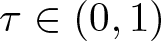$\tau\in(0,1)$ and $j_0\in\mathbb{N}$ such that

\begin{equation*}\left\|u(\cdot,t)-m\right\|_{L^q(\Omega)}\geqslant\frac{1}{4}\|u^*\|_{L^q(\Omega)}\end{equation*}

for all $t\in[t_j,t_{j}+\tau]$ and each $j\geqslant j_0$ which in particular implies that for any $j\geqslant j_0$ we have

(4.14)\begin{equation} \int_{t_j}^{t_j+\tau}\left\|u-m\right\|_{L^q(\Omega)}^{2}ds\geqslant\frac{\tau}{16}\|u^*\|^2_{L^q(\Omega)}. \end{equation}

From lemma 4.3, we derive

\begin{align*} \int_{t_j}^{t_{j}+\tau}\left\|u-m\right\|_{L^q(\Omega)}^{2}ds\leqslant\int_{t_j}^{+\infty}\left\|u-m\right\|_{L^q(\Omega)}^{2}ds\rightarrow0 \end{align*}

as $j\rightarrow+\infty$ which contradicts (4.14). Hence, (4.12) is verified. Similarly, we can show that (4.13) holds.

Step 2: We use the L’Hôpital rule to find

\begin{equation*}\lim_{s\rightarrow m}\frac{s-m-m\ln\frac{s}{m}}{(s-m)^2}=\lim_{s\rightarrow m}\frac{1-\frac{m}{s}}{2(s-m)}=\lim_{s\rightarrow m}\frac{1}{2s}=\frac{1}{2m},\end{equation*}

which implies that there exists a constant $\xi_1 \gt 0$ such that for all $|s-m|\leqslant\xi_1$

(4.15)\begin{equation} \frac{1}{4m}(s-m)^2\leqslant s-m-m\ln \frac{s}{m}\leqslant\frac{1}{m}(s-m)^2. \end{equation}

From the result in Step 1, we find a constant $T_1 \gt 0$ such that

\begin{equation*} \|u-m\|_{L^\infty(\Omega)}\leqslant\xi_1\quad\text{for all}\ t \gt T_1 \end{equation*}

which, together with (4.15), gives

(4.16)\begin{equation} \frac{1}{4m}\int_\Omega(u-m)^2\leqslant\int_\Omega \left(u-m-m\ln \frac{1}{m}\right)\leqslant\frac{1}{m}\int_\Omega(u-m)^2\quad\text{for all}\ t \gt T_1. \end{equation}

Step 3: Case of $\alpha\geqslant2$. Substituting (4.16) into (4.2), we find a constant $C_2 \gt 0$ such that

\begin{equation*} \begin{aligned} &\frac{d}{{dt}}\left(\int_\Omega\left(u-m-m\ln\frac{u}{m}\right)+A\sum\limits_{i = 1}^k {\int_\Omega {{{\left( {{v_i} - m} \right)}^2}}}+B\int_\Omega {{{\left| {\bf{w}} \right|}^2}}\right)\\ \leqslant&-C_2\left(\int_\Omega\left(u-m-m\ln\frac{u}{m}\right)+A\sum\limits_{i = 1}^k {\int_\Omega {{{\left( {{v_i} - m} \right)}^2}} }+B\int_\Omega {{{\left| {\bf{w}} \right|}^2}}\right) \quad \text{for all}\ t \gt T_1 \end{aligned} \end{equation*}

which warrants a constant $C_3 \gt 0$ such that

\begin{equation*}\int_\Omega\left(u-m-m\ln\frac{u}{m}\right)+A\sum\limits_{i = 1}^k {\int_\Omega {{{\left( {{v_i} - m} \right)}^2}} }+B\int_\Omega {{{\left| {\bf{w}} \right|}^2}}\leqslant C_3e^{-C_2t}\quad\text{for all}\ t \gt T_1.\end{equation*}

Hence, noticing (4.16), this gives a constant $C_4 \gt 0$ such that

(4.17)\begin{equation} \int_\Omega (u-m)^2+\sum\limits_{i = 1}^k {\int_\Omega {{{\left( {{v_i} - m} \right)}^2}} }+\int_\Omega {{{\left| {\bf{w}} \right|}^2}}\leqslant C_4e^{-C_2t}\quad\text{for all}\ t \gt T_1. \end{equation}

The Gagliardo–Nirenberg inequality yields a constant $C_5 \gt 0$ such that

\begin{equation*} \|u-m\|_{L^{\infty}(\Omega)} \leqslant C_5\|u-m\|_{W^{1, \infty}(\Omega)}^{\frac{n}{n+2}}\|u-m\|_{L^{2}(\Omega)}^{\frac{2}{n+2}} \end{equation*}

which, together with (4.17) and (4.1), implies the desired result.

Step 4: Case of $2-\frac{n}{2} \lt \alpha \lt 2$. Thanks to the second equation of (1.1), we have

\begin{equation*}\frac{d}{dt}(\overline{v_1}-m)+(\overline{v_1}-m)=(\overline{u}-m)\quad\text{for all }t \gt 0,\end{equation*}

and hence

\begin{equation*}\overline{v_1(t)}-m=e^{-t}\left(\overline{v_1(0)}-m\right)+\int_0^te^{-(t-s)}\left(\overline{u(s)}-m\right)ds\quad\text{for all }t \gt 0.\end{equation*}

Since

\begin{equation*}\left\|u\left(\cdot,t\right)-m\right\|_{L^{\infty}\left(\Omega\right)}\rightarrow0\quad\text{as }t\rightarrow+\infty,\end{equation*}

then for any ɛ > 0 there exists $T_2 \gt 0$ such that

\begin{equation*}\left|\overline{u\left(t\right)}-m\right|\leqslant\varepsilon\quad\text{for all }t \gt T_2,\end{equation*}

which infers

\begin{equation*}\left|\int_{T_2}^te^{-(t-s)}\left(\overline{u(s)}-m\right)ds\right|\leqslant\varepsilon\int_{T_2}^te^{-(t-s)}ds\leqslant\varepsilon\quad\text{for all }t \gt T_2.\end{equation*}

According to lemma 4.1, we find a constant $C_7 \gt 0$ such that

\begin{equation*}\left|\overline{u\left(s\right)}-m\right|\leqslant C_7\quad\text{for all }s\in[0,T_2],\end{equation*}

which implies

\begin{equation*}\left|\int_0^{T_2}e^{-(t-s)}\left(\overline{u(s)}-m\right)ds\right|\leqslant C_7(e^{T_2}-1)e^{-t}.\end{equation*}

Therefore, there exists $T_3 \gt T_2$ such that

\begin{equation*}\left|\int_0^{T_2}e^{-(t-s)}\left(\overline{u(s)}-m\right)ds\right|\leqslant\varepsilon\quad\text{for all }t \gt T_3.\end{equation*}

Hence, it holds that

\begin{align*} & \left|\int_0^te^{-(t-s)}\left(\overline{u(s)}-m\right)ds\right|\\ & \quad =\left|\int_0^{T_2}e^{-(t-s)}\left(\overline{u(s)}-m\right)ds+\int_{T_2}^te^{-(t-s)}\left(\overline{u(s)}-m\right)ds\right|\\ &\quad \leqslant\left|\int_0^{T_2}e^{-(t-s)}\left(\overline{u(s)}-m\right)ds\right|+\left|\int_{T_2}^te^{-(t-s)}\left(\overline{u(s)}-m\right)ds\right|\\ &\quad \leqslant2\varepsilon\quad\text{for all }t \gt T_3, \end{align*}

which, along with $e^{-t}\left(\overline{v_1(0)}-m\right)\rightarrow 0$ as $t\rightarrow+\infty$, implies

\begin{equation*}\overline{v_1(t)}-m\rightarrow0\quad\text{as }t\rightarrow+\infty.\end{equation*}

Similarly, we get that for $i=2,3,\ldots,k$,

\begin{equation*}\overline{v_i(t)}-m\rightarrow0\quad\text{as }t\rightarrow+\infty,\end{equation*}

which, together with

\begin{equation*}\sum\limits_{i = 1}^k \left\|v_i\left(\cdot ,t\right)-\overline{v_i(t)}\right\|_{L^{\infty}\left(\Omega\right)}\rightarrow0\quad\text{as }t\rightarrow+\infty,\end{equation*}

infers

\begin{equation*}\sum\limits_{i = 1}^k \left\|v_i\left(\cdot ,t\right)-m\right\|_{L^{\infty}\left(\Omega\right)}\rightarrow0\quad\text{as }t\rightarrow+\infty.\end{equation*}

Step 5: According to the condition (1.6) we have

\begin{equation*}\frac{m}{4} \lt \frac{2(k+1)}{k}K_1\mu m^{\alpha-2},\end{equation*}

which implies that there exist $\widehat{\eta} \gt 0$ and $\widehat{\xi} \gt 0$ such that

(4.18)\begin{equation} \frac{m}{4} \lt \widehat{\eta} \lt 2\widehat{\xi} \lt \frac{2(k+1)}{k}K_1\mu m^{\alpha-2}. \end{equation}

The combination of (4.3), (4.4), and (4.6) implies

(4.19)\begin{equation} \begin{aligned} &\frac{d}{{dt}}\left(\int_\Omega {{\left( {u - m - m\ln \frac{u}{m}} \right)}} +\widehat{\xi}\sum\limits_{i = 1}^k {\int_\Omega {{{\left( {{v_i} - m} \right)}^2}} } + \widehat{\eta} \int_\Omega {{{\left| {\bf{w}} \right|}^2}}\right) \\ \leqslant& -m\int_\Omega {\frac{{{{\left| {\nabla u} \right|}^2}}}{{{u^2}}}} + m\int_\Omega \frac{{\bf{w}}\cdot \nabla u}{u} -\widehat{\eta} \int_\Omega {{{\left| {\mathbf{w}} \right|}^2}} - 2\widehat{\xi}\sum\limits_{i = 1}^{k - 1} {\int_\Omega {{{\left| {\nabla {v_i}} \right|}^2}} } - \left( {2\widehat{\xi}-\widehat{\eta}} \right)\int_\Omega {{{\left| {\nabla {v_k}} \right|}^2}} \\ &\quad -\mu\int_\Omega {\left( {u - m} \right)\left( {{u^{\alpha - 1}}-{m^{\alpha-1}}} \right)} - 2\widehat{\xi}\sum\limits_{i = 1}^k {\int_\Omega {{{\left( {{v_i} - m} \right)}^2}} } \\ &\quad+ 2\widehat{\xi} \int_\Omega {\left( {u - m} \right)\left( {{v_1} - m} \right)}+ 2\widehat{\xi} \sum\limits_{i = 2}^k {\int_\Omega {\left( {{v_i} - m} \right)\left( {{v_{i - 1}} - m} \right)} } \quad \text{for all}\ t \gt 0. \end{aligned} \end{equation}

Thanks to (4.12), we find $T_4 \gt T_3$ such that

\begin{equation*}0\leqslant u(x,t)\leqslant 2m \quad\mbox{for all}\ x\in\Omega,\ t \gt T_4.\end{equation*}

An application of lemma 2.4 yields a constant $K_1 \gt 0$ such that

\begin{equation*} \left(\left(\frac{u}{m}\right)^{\alpha-1}-1\right)\left(\frac{u}{m}-1\right)\geqslant K_1\left(\frac{u}{m}-1\right)^2 \quad\text{for any}\ u\in[0,2m], \end{equation*}

i.e.

\begin{equation*} \left(u^{\alpha-1}-m^{\alpha-1}\right)\left(u-m\right)\geqslant K_1m^{\alpha-2}\left(u-m\right)^2 \quad\text{for any}\ u\in[0,2m], \end{equation*}

which along with (4.19), yields

\begin{equation*} \begin{aligned} &\frac{d}{{dt}}\left(\int_\Omega {{\left( {u - m - m\ln \frac{u}{m}} \right)}} +\widehat{\xi}\sum\limits_{i = 1}^k {\int_\Omega {{{\left( {{v_i} - m} \right)}^2}} } + \widehat{\eta} \int_\Omega {{{\left| {\bf{w}} \right|}^2}}\right) \\ \leqslant& -m\int_\Omega {\frac{{{{\left| {\nabla u} \right|}^2}}}{{{u^2}}}} + m\int_\Omega \frac{{\bf{w}}\cdot \nabla u}{u} - \widehat{\eta} \int_\Omega {{{\left| {\mathbf{w}} \right|}^2}} - 2\widehat{\xi}\sum\limits_{i = 1}^{k - 1} {\int_\Omega {{{\left| {\nabla {v_i}} \right|}^2}} } - \left({2\widehat{\xi}-\widehat{\eta}}\right)\int_\Omega {{{\left| {\nabla {v_k}} \right|}^2}} \\ &\quad -K_1\mu m^{\alpha-2}\int_\Omega\left(u-m\right)^2- 2\widehat{\xi}\sum\limits_{i = 1}^k {\int_\Omega {{{\left( {{v_i} - m} \right)}^2}} } \\ &\quad+ 2\widehat{\xi} \int_\Omega {\left( {u - m} \right)\left( {{v_1} - m} \right)}+ 2\widehat{\xi} \sum\limits_{i = 2}^k {\int_\Omega {\left( {{v_i} - m} \right)\left( {{v_{i - 1}} - m} \right)} }\\ \leqslant&-\int_\Omega X\widehat{S}X^T-\left( {2\widehat{\xi}-\widehat{\eta}}\right)\int_\Omega{{{\left| {\nabla {v_k}} \right|}^2}}-\int_\Omega Z\widehat{T}Z^T\quad \text{for all}\ t \gt T_4, \end{aligned} \end{equation*}

where $X=\left(\frac{|\nabla u|}{u},|\textbf{w}|\right)$, $Z=\left(u-m,v_1-m,v_2-m,\ldots,v_k-m\right)$,

\begin{equation*}\widehat{S}= \begin{bmatrix} m&-\frac{m}{2} \\ -\frac m 2& \widehat{\eta} \end{bmatrix}\quad \text{and}\quad \widehat{T}= \begin{bmatrix} K_1\mu m^{\alpha-2}&-\widehat{\xi}&0&\cdots &0 \\ -\widehat{\xi}&2\widehat{\xi}&-\widehat{\xi}&\cdots&0\\ \vdots & \vdots & \vdots & \ddots & \vdots \\ 0&0&0& \cdots &2\widehat{\xi} \end{bmatrix}.\end{equation*}

Using (4.18), we get that $\widehat{S}$ and $\widehat{T}$ are positive definite as the argument of Step 2 in the proof of the positive definite of T in lemma 4.3. Therefore, we obtain a constant $C_8 \gt 0$ such that

\begin{equation*} \begin{aligned} &\frac{d}{{dt}}\left(\int_\Omega {{\left( {u - m - m\ln \frac{u}{m}} \right)}} +\widehat{\xi}\sum\limits_{i = 1}^k {\int_\Omega {{{\left( {{v_i} - m} \right)}^2}} } + \widehat{\eta} \int_\Omega {{{\left| {\bf{w}} \right|}^2}}\right) \\ \leqslant&-C_8\left(\int_\Omega\left(u-m\right)^2 +\widehat{\xi}\sum\limits_{i=1}^k\int_\Omega\left(v_i-m\right)^2+\widehat{\eta}\int_\Omega\left|{\bf{w}}\right|^2\right)\quad \text{for all}\ t \gt T_4. \end{aligned} \end{equation*}

Similar to the argument in Step 2 and Step 3, we can get constants $C_9,C_{10} \gt 0$ satisfying

\begin{align*}&\left\|{u\left(\cdot,t\right)-m}\right\|_{L^\infty\left(\Omega \right)}+\sum\limits_{i = 1}^k\left\|v_i\left(\cdot ,t\right)-m\right\|_{L^\infty\left(\Omega\right)}+\left\| {\bf{w}}\left(\cdot,t\right)\right\|_{L^\infty\left(\Omega\right)} \\ & \quad \leqslant C_9e^{-C_{10}t}\quad\text{for all}\ t \gt T_4,\end{align*}

which along with the continuity of the solution in $[0,T_4]$, completes the proof of the theorem.