





1. Introduction
The heat exchange between a solid body and the surrounding environment can be enhanced by forcing a fluid to flow over the surface of the body. As such, the problem of determining the heat transfer performances of a cooling system naturally pertains to fluid mechanics. In many applications, a simple way of forcing a fluid to flow over a solid surface is by directing a jet flow towards a target plate. The impingement of a jet onto a solid wall determines a complex flow configuration which is commonly distinguished in several regions based on the local characteristics of the flow (Jambunathan et al. Reference Jambunathan, Lai, Moss and Button1992). Referring to the two-dimensional sketch in figure 1, the fluid flow exits from an orifice of characteristic size
 $D$
placed at a normal distance
 $H$
from the impingement plate. For a sufficiently large separation between the nozzle exit section and the impingement plate (i.e. for sufficiently large
 $H/D$
ratios), a region exists where the jet exhibits features that closely resemble those of a free-jet flow. In this region, the jet core is characterised by small turbulence fluctuations compared with the free-shear layer that develops between the jet and the outer quiescent fluid. For a jet impinging normally onto a flat plate, the intersection of the jet axis with the impingement plate is a stagnation point and its surrounding region is usually termed the stagnation region or impingement region. The free-jet fluid approaching the stagnation region experiences a strong adverse pressure gradient and gets deflected to flow along the impingement plate where a radial wall jet develops.
Impinging jets and their heat transfer characteristics have been of great research interest in the past due to the broad range of engineering applications that use impinging jets as a means for removing heat or for drying surfaces. In view of these applications, most of the work in the literature aims to characterise the flux at the impingement plate of a transported scalar quantity under varying operating conditions. In case of heat transfer analysis, the scalar field represents the fluid temperature and the assessment of its wall flux determines the amount of heat exchanged between the fluid and the impingement plate. The characterisation of mean wall heat transfer in impinging jets is well established, with several heat transfer correlations developed to relate flow geometry and operating regimes to the distribution of mean wall heat transfer (see for instance the recent review of Uddin et al. Reference Uddin, Kee and Weigand2024).
Yet, the knowledge of the mean wall heat transfer distribution does not alone allow for a decision on the merit of a heat transfer device, for it is important to also consider the power input required to drive the flow through the system. In impinging jets, this aspect is usually looked upon only when a comparison between the heat transfer performances of different configurations is of interest (Brignoni & Garimella Reference Brignoni and Garimella2000; Gao et al. Reference Gao, Sun and Ewing2003; Cafiero et al. Reference Cafiero, Discetti and Astarita2014). Nonetheless, the evaluation of the mechanical energy expenditure and its comparison with the amount of exchanged heat in a simple configuration can be relevant from a fundamental perspective.
In forced convection, the ratio between the exchanged thermal power and the driving power input is also a representative measure of the similarity between momentum and heat transfer (Secchi et al. Reference Secchi, Gatti, Piomelli and Frohnapfel2025). From this perspective, the analysis of the thermal efficiency coincides with the assessment of the Reynolds analogy, which states that momentum and heat exchange occur similarly in a flow of a fluid having a unit Prandtl number, where the Prandtl number,
 $Pr=\nu /\alpha$
, represents the ratio between the momentum and the thermal molecular diffusivities of the fluid (i.e. the kinematic viscosity
 $\nu$
and the thermal diffusivity
 $\alpha$
, respectively). In forced convection, this analogy can be measured through the Reynolds analogy factor,
 $RA=2C_h/C_f$
, where
 $C_f$
and
 $C_h$
are, respectively, the friction and heat transfer coefficients (the latter is also known as the Stanton number). For
 $Pr=1$
, and in the absence of strong pressure gradients, the Reynolds analogy factor is expected to be
 $RA\approx 1$
; for instance, this is verified for zero-pressure-gradient boundary-layer flows (Schlichting & Gersten Reference Schlichting and Gersten2000).
(a) sketch of the relevant regions of an impinging jet flow; (b) sketch of the computational domain with the relevant geometrical parameters.

Impinging jets are a typical example of a complex flow for which the Reynolds analogy cannot be used as a basis for estimating the wall heat transfer from knowledge of the momentum wall flux (Bunker Reference Bunker2013; Woodworth et al. Reference Woodworth, Salazar and Liu2023). Within the stagnation region, a departure from perfectly analogous momentum and heat transfer at the impingement plate is verified, as a vanishingly small wall-shear stress occurs close to the jet axis, in spite of a non-vanishing wall heat flux. Further downstream of the stagnation region, a return towards similar heat and momentum transfers might be expected, provided that the flow is not subject to strong pressure gradients and analogous boundary conditions apply for the velocity and the temperature field (Wilke & Sesterhenn Reference Wilke and Sesterhenn2017).
Although the assessment of the Reynolds analogy along the impingement plate can be instructive for understanding how dissimilar heat and momentum transfers are locally, no information can be ascertained from it regarding the thermal efficiency of the system. This is in contrast to forced convection problems, where the
 $RA$
actually links the mechanical power required to pump the flow and the thermal power that can be extracted from the system. For instance, in pipe or channel flow, the friction and heat transfer coefficients can easily be related to the pumping and thermal power, respectively. This interpretation, which was introduced by Dipprey & Sabersky (Reference Dipprey and Sabersky1963) in the analysis of heat transfer over surface roughness in pipe flow, ceases to be applicable in the case of an impinging jet. For this flow, the total thermal power extracted from the impingement plate is determined by the surface integral of the wall heat flux, and hence it is related to the heat transfer coefficient; conversely, a similar relationship does not hold between the wall friction and the mechanical power required to pump the flow through the system.
In this work, direct numerical simulation (DNS) data are used to compare the mechanical energy expenditure with the thermal power that is exchanged at the impingement plate in different regions of the flow. While the exchanged thermal power is computed in a straightforward manner, as the surface integral of the wall heat flux, an integral balance of the total mechanical energy, viz. the sum of kinetic energy and pressure work, is used to compute the bulk mechanical energy dissipation. The latter coincides with the mechanical energy expenditure within the control volume over which the integral analysis is applied. Further, following the recent analysis of Secchi et al. (Reference Secchi, Gatti, Piomelli and Frohnapfel2025), the mechanical energy budget is compared with the balance equation for
 $\varGamma =\theta ^2/2$
, where
 $\theta$
represents a non-dimensional scalar temperature field. In this work, the field
 $\varGamma$
will be referred to as the squared-scalar field. Application of the integral control-volume analysis to the equation for
 $\varGamma$
allows the exchanged thermal power at the impingement plate to be related to the bulk dissipation of the scalar field, thus enabling a direct assessment of how similarly the total mechanical energy and
 $\varGamma$
are dissipated within the bulk of the flow. This analysis is further used to suggest possible connections between the non-unitary thermal efficiencies and local flow phenomena.
The description of the flow configuration and of the numerical method is provided in § 2 of this manuscript, whereas § 3 is dedicated to presenting the results of the investigation. In particular, the analysis of the energetics of the impinging jet is preceded by the description of the mean-flow field, with significant attention to the flow topology and to the effects determined by the different boundary values enforced on the velocity and temperature fields. The main findings of the present work are summarised in § 4.
2. Methodology
A sketch of the flow configuration is reported in figure 1 along with its important geometrical parameters. A turbulent jet issues from a fully developed turbulent pipe flow having a diameter
 $D$
and a mean bulk velocity
 $U_b$
. The Reynolds number is set to
 ${\textit{Re}}=U_bD/\nu =5300$
. The target plate is located at a distance
 $H=2D$
from the pipe exit section and is orthogonal to the jet axis. An additional confinement plate is placed, parallel to the impingement plate, at the same height as the pipe exit section. The confinement plate prevents the entrainment of outer flow, reducing the required domain size, and is commonly used in practical applications where heat needs to be removed within a closed environment.
The flow is governed by the incompressible Navier–Stokes equations
 \begin{align} \boldsymbol{\nabla }\boldsymbol{\cdot }\boldsymbol{u} & = 0, \end{align}
 \begin{align} \frac {\partial \boldsymbol{u}}{\partial t} + \boldsymbol{\nabla }\boldsymbol{\cdot }\left ( \boldsymbol{u}\otimes \boldsymbol{u}\right ) & = -\frac {1}{\rho }\boldsymbol{\nabla }p + \nu{\nabla} ^2\boldsymbol{u}, \end{align}
which are augmented by including a transport equation for the passive scalar field
 $\theta$
 \begin{align} \frac {\partial \theta }{\partial t} + \boldsymbol{\nabla }\boldsymbol{\cdot }(\boldsymbol{u}\theta ) = \alpha{\nabla} ^2 \theta . \end{align}
In the equations,
 $t$
denotes the time and
 $\boldsymbol{u}$
indicates the velocity vector; the pressure and the fluid density are denoted respectively by
 $p$
and
 $\rho$
. In the context of heat transfer analysis, the scalar field
 $\theta$
is typically identified as the temperature field of the fluid provided that temperature variations remain sufficiently small for buoyancy effects to be negligible and for fluid properties to remain constant. We shall proceed with the investigation by maintaining this assumption and by identifying the scalar field
 $\theta = (T - T_j)/(T_w - T_j)=(T - T_j)/\Delta T$
, where
 $T$
indicates the fluid temperature, and
 $T_w$
and
 $T_j$
represent, respectively, the impingement plate and jet prescribed temperatures, and
 $\Delta T = T_w - T_j$
. Further, unless explicitly stated, a unit Prandtl number is considered for all the results reported in this work.
Equations (2.1), (2.2) and (2.3) are numerically integrated using the flow-solver Nek5000 (Argonne National Laboratory 2019), based on the spectral element method proposed by Patera (Reference Patera1984). The governing equations are cast in their weak form through the Galerkin formalism. The solution and test function spaces are identified with the finite-dimensional space spanned by Lagrange polynomials of degree
 $N$
based on Gauss–Legendre–Lobatto (GLL) nodes in the unit cubic element
 $[-1, \, 1]^3$
. In particular, in the present study, the same polynomial degree is used for the pressure and velocity spaces i.e. a
 $\mathrm{P}_N-\mathrm{P}_N$
formulation. The computational domain
 $[-L_x/2, L_x/2] \times [-L_y/2, L_y/2] \times [0, H]$
is discretised into
 $E$
elements on which Gaussian quadrature on GLL nodes is used to approximate the integrals arising from the weak formulation of the problem and to assemble the discretised system of equations.
The computational mesh is displayed in panels (a) and (b) of figure 2; element stretching is applied in the wall-normal direction to cluster elements toward the impingement and confinement plates. Further, the mesh is designed to have a uniform in-plane element distribution in the square
 $[-4D, \, 4D]\times [-4D, \, 4D]$
. The mesh parameters and the total number of degrees of freedom (
 ${\textit{DOF}}$
) are reported in table 1. The
 ${\textit{DOF}}$
corresponds to the number of grid points in the physical space and is given by
 ${\textit{DOF}}=E\times (N+1)^3$
. Further, referring to table 1, the numbers of elements in the wall-parallel directions,
 $x$
and
 $y$
, are given by
 $2\times n_{\textit{xe}}+ n_{\textit{xc}}$
, and
 $2\times n_{\textit{ye}}+ n_{\textit{yc}}$
, respectively, where the subscripts
 $c$
and
 $e$
indicate the central and external regions of the mesh. The number of elements in the wall-normal direction is denoted by
 $n_z$
.
Simulation parameters.

Table 1. Long description
A table with one row and twelve columns displaying computational mesh parameters and degrees of freedom. The columns are labeled as follows: Lx/D, Ly/D, H/D, nxc, nx, nxc, nyc, nz, E, N, DOF, TavguUb/D. The row contains the following values: 16, 16, 2, 98, 29, 98, 29, 48, 1168128, 7, 598 x 10^6, 500.
Computational mesh of elements; (a) top view; (b) front view for
 $x \in [-5, \, 5]$
. To ease the visualisation, only one in every two elements is shown in the figures. (c) Average local grid size to Kolmogorov length scale ratio,
 $\varDelta /\eta _K$
. (d) Average time step size to Kolmogorov time scale ratio,
 $\Delta t/\tau$
.

A polynomial degree
 $N=7$
has been used for all the results reported in this study. This choice allows for the matching of the DNS resolution requirements everywhere in the flow field. This is shown in figure 2(c), which depicts the ratio
 $\varDelta / \eta _K$
, where
 $\varDelta = (\Delta x \Delta y \Delta z)^{1/3}$
, with
 $\Delta x, \, \Delta y$
and
 $\Delta z$
being the local grid spacings in the coordinate directions, represents a measure of the local grid size, and
 $\eta _K= ( \nu ^3 / \varepsilon )^{1/4}$
is the Kolmogorov length scale. Here,
 $\varepsilon = 2\nu \langle \boldsymbol{s}^\prime : \boldsymbol{s}^\prime \rangle$
represents the mean dissipation rate of turbulent kinetic energy, where
 $\boldsymbol{s}$
denotes the strain rate tensor,
 $\boldsymbol{s} = ( \boldsymbol{\nabla }\otimes \boldsymbol{u} + \boldsymbol{\nabla }\otimes \boldsymbol{u}^T )/2$
. Here, and in the following, time and spatial averaging in the azimuthal direction is denoted by angular brackets
 $\langle \, \boldsymbol{\cdot }\, \rangle$
and a prime superscript
 $ ( \boldsymbol{\cdot })^\prime$
indicates fluctuations with respect to the time and azimuthal mean of a given quantity.
In a similar fashion, the time resolution is checked by computing the ratio between the average time step size,
 $\Delta t$
, used to advance the discretised equations, to the local Kolmogorov time scale,
 $\tau = (\nu /\varepsilon )^{1/2}$
. The result, which is reported in figure 2(d), shows that the adopted time step size remains significantly smaller than the Kolmogorov time scale in every region of the flow, even in the shear layers of the free and wall jets where the Kolmogorov time scale reaches its minima. Although larger time step sizes were possible without compromising the resolution of the dissipative scales, for numerical stability the time step size was limited in order to achieve a Courant-Friedrichs-Lewy number, CFL
 $ = 0.8$
.
(a) Mean Nusselt number distribution along the impingement plate.
 , present DNS,
 $N=7$
; blue symbols, present DNS,
 $N=5$
; black symbols, experimental data of Lee & Lee (Reference Lee and Lee2000). (b) Mean axial velocity profile at the inflow section of the jet domain (symbols); DNS data of Pirozzoli et al. (Reference Pirozzoli, Romero, Fatica, Verzicco and Orlandi2021) (solid line).

The independence of the results from the adopted grid was checked by comparing the numerical solutions for
 $N=5$
and
 $N=7$
on a fixed mesh of elements. As an example, figure 3(a) displays the time- and space-averaged Nusselt number distribution along the impingement plate for the two solutions and compares them with the experimental measurements of Lee & Lee (Reference Lee and Lee2000). The Nusselt number is defined as
 $Nu= q_w D /(\lambda \Delta T)$
, where
 $q_w$
denotes the wall heat flux, and
 $\lambda$
is the coefficient of thermal conductivity of the fluid. Here, and in the following,
 $r$
denotes the radial distance from the jet axis and
 $z$
measures the distance from the impingement plate. In addition to suggesting the grid independence of the results, figure 3(a) shows that the present data match experimental data reasonably well. In this respect, we note that the observed differences can be attributed to difficulties in replicating exactly the conditions at the boundary of the experimental set-up.
Time advancement is performed semi-implicitly using a third-order backward differencing and extrapolation scheme. More specifically, the advective nonlinear terms of the discretised momentum equation are extrapolated using a third-order extrapolation scheme, whereas the viscous terms are implicitly advanced using a third-order backward differencing formula. An operator splitting technique is employed to decouple the pressure and velocity computation. As a result, at each time step the problem is split into solving one pressure Poisson equation and a Helmholtz system for each velocity component. Once the velocity field has been computed, an additional Helmholtz system needs to be solved for each simulated passive scalar field. After reaching statistically stationary conditions, data acquisition for computing time statistics has been carried out for
 $T_{\textit{avg}}\approx 500 D/U_b$
.
No-slip boundary conditions for the velocity field are prescribed on the impingement and confinement plates, whereas at the inflow section of the computational domain (i.e. at the nozzle exit section) a turbulent velocity field is interpolated at each time step from a cross-section of a fully developed turbulent pipe flow simulation. Figure 3(b) shows the comparison of the mean axial velocity profile at the inflow section of the jet domain with the DNS data of Pirozzoli et al. (Reference Pirozzoli, Romero, Fatica, Verzicco and Orlandi2021) for pipe flow at a friction Reynolds number
 ${\textit{Re}}_\tau =180$
(which corresponds to a bulk Reynolds number,
 ${\textit{Re}}=5300$
). A
 $+$
superscript is used to denote viscous units-scaled quantities.
For the scalar temperature field
 $\theta$
, Dirichlet boundary conditions are prescribed on the impingement and confinement plates and on the inflow section of the domain. In particular, the confinement plate is assumed to be at thermal equilibrium with the issuing jet; therefore
 $\theta =0$
is prescribed on the confinement plate and on the nozzle exit section. On the impingement plate the temperature is assigned to be equal to a constant value
 $T_w$
and, consequently, the boundary condition for the scalar field is
 $\theta =1$
on the impingement wall. In the following,
 $\theta _w$
will be used to denote the prescribed value of
 $\theta$
at the impingement plate. On the lateral open boundaries of the computational domain, the energy-stable boundary conditions proposed by Dong (Reference Dong2015) and Liu et al. (Reference Liu, Xie and Dong2020) are applied, respectively, for the velocity and the temperature fields.
The presence of an artificial open boundary in the simulation naturally raises the question of whether the size of the computational domain has any influence on the flow statistics. To check on this, an additional simulation with similar resolution was run on a larger computational box having size
 $L_x=20D$
and
 $L_y=20D$
. Although the simulation was run for a shorter period of time to save computational resources, a good agreement is observed between the statistics computed from the solutions obtained using the two domains of different lateral extent, suggesting the independence of the results on the location of the artificial open boundary. For instance, figure 4 shows the the radial distribution of Reynolds stresses sampled at a wall-normal distance
 $z=0.1D$
.
Radial distribution of Reynolds stresses sampled at
 $z=0.1D$
.
 ,
 $\langle u_r^\prime u_r^\prime \rangle /U_b^2$
;
 ,
 $\langle u_\phi ^\prime u_\phi ^\prime \rangle /U_b^2$
;
 ,
 $\langle u_z^\prime u_z^\prime \rangle /U_b^2$
;
 ,
 $\langle u_r^\prime u_z^\prime \rangle /U_b^2$
. Solid lines correspond to the computational domain with
 $L_x=L_y=16D$
; symbols correspond to
 $L_x=L_y=20D$
.

3. Results
3.1. Mean-flow topology
Visualisation of the mean velocity field. (a) Mean radial velocity
 $\langle u_r \rangle /U_b$
; (b) mean axial velocity
 $\langle u_z \rangle /U_b$
. Panels (c) and (d) depict streamlines of the mean velocity field. Streamlines are colour coded to identify regions of positive (orange) and negative (blue) values of the mean radial velocity
 $\langle u_r \rangle$
, panel (c), and of the mean axial velocity
 $\langle u_z \rangle$
, panel (d).

The mean-flow field is visualised in figure 5 through colour maps of the mean radial and axial velocity components, respectively,
 $\langle u_r \rangle$
and
 $\langle u_z \rangle$
, together with their streamlines. Panels (a) and (b) in the figure highlight the free-jet region, which is characterised by a strong negative axial velocity, and the wall jet region, in which the mean flow develops radially along the impingement plate. Structurally, the mean flow is characterised by a large-scale recirculating cell which can be observed in the mean streamline patterns reported in figures 5(c) and 5(d). This recirculating structure has its centre at
 $r\approx 5.4D$
and
 $z\approx D$
and originates from the continuous momentum supply through the wall jet and the presence of the no-slip boundary condition on the confinement and impingement plates. In figure 6(a), the presence and the centre of such a recirculating cell is confirmed by comparing streamlines of the mean flow with particle image velocimetry measurements from Chen et al. (Reference Chen, Yang, Huang, Zhou, Zhang and Wang2024). A second recirculating zone is observed close to the open boundary of the computational domain. Due to its presence, inflow and outflow occur across the bottom and top halves of the open boundary, respectively. Nevertheless, the velocity magnitude in this region only reaches a few per cent,
 $\lesssim 5\,\%$
, of the mean bulk velocity in the free jet.
(a) Streamlines of the mean velocity field. Solid black lines, present DNS; red dots, data from Chen et al. (Reference Chen, Yang, Huang, Zhou, Zhang and Wang2024). (b) Mean radial velocity and temperature profiles at different radial locations.
 ,
 $\langle u_r \rangle /U_b$
;
 ,
 $\langle \theta \rangle$
; symbols indicate the maxima and minima of, respectively, the mean radial velocity and temperature profiles. Vertical black dashed lines indicate the radial location at which the profiles are sampled. (c) Boundary-layer thicknesses.
 ,
 $z_m/D$
;
 ,
 $z_{\theta m}/D$
;
 ,
 $z_{\varTheta m}/D$
. (d) Radial distribution of the maxima of the mean radial velocity profiles.
 , present DNS; red squares, Chen et al. (Reference Chen, Yang, Huang, Zhou, Zhang and Wang2024);
 , 1.12/(r/D).

Figure 6. Long description
Panel A: A contour plot showing streamlines of the mean velocity field. The x-axis is labeled r/D and ranges from 0 to 8. The y-axis is labeled z/D and ranges from 0 to 2. Solid black lines represent present DNS data, and red dots represent data from Chen et al. (2024). Panel B: A line graph showing mean radial velocity and temperature profiles at different radial locations. The x-axis is labeled r/D and ranges from 0 to 8. The y-axis is labeled z/D and ranges from 10^-2 to 10^0. Different colored lines represent different profiles, with symbols indicating the maxima and minima. Vertical black dashed lines indicate the radial location at which the profiles are sampled. Panel C: A line graph showing boundary-layer thicknesses. The x-axis is labeled r/D and ranges from 0 to 8. The y-axis is labeled z/D and ranges from 0 to 0.2. Different colored lines represent different boundary-layer thicknesses. Panel D: A line graph showing the radial distribution of the maxima of the mean radial velocity profiles. The x-axis is labeled r/D and ranges from 1 to 8. The y-axis is labeled um/Ub and ranges from 10^-2 to 10^0. Black lines represent present DNS data, red squares represent data from Chen et al. (2024), and a dashed line represents the equation 1.12/(r/D).
The development of the mean flow along the radial direction is further analysed in figure 6(b), which shows mean radial velocity and temperature profiles at several radial stations. The mean profiles represent well the characteristic shape of a wall jet that is generated by the injection of high-momentum fluid through a narrow gap between a solid wall and a quiescent fluid. Such a momentum inflow determines a two-layered flow in which the maximum velocity is attained in a region of the flow bounded by an inner wall-boundary layer and an outer free-shear flow. In the present case, it must be noted that the outer region of the flow is not characterised by a perfectly quiescent fluid, but rather, by a mild backflow which is induced, in the upper part of the domain, by the primary recirculating cell that was observed in the analysis of figure 5(c, d). Due to the recirculating flow, a wall jet also develops on the confinement plate, whose direction opposes that developing along the impingement plate, and with comparatively little streamwise momentum.
Due to the different boundary values that
 $\langle u_r \rangle$
and
 $\langle \theta \rangle$
have on the impingement plate, their mean profiles differ significantly from each other everywhere in the domain. In the wall jet along the bottom plate, high-momentum cold fluid, coming from the jet, determines that the mean temperature profiles have their minima over the same region where the mean radial velocity profiles are maximal. In the upper part of the domain, the recirculating flow carries warm fluid to flow over the confinement plate. Figure 6(b) shows that, in the bottom wall jet, the mean radial velocity maxima,
 $u_m$
and the mean temperature minima,
 $\theta _m$
, occur at significantly different wall-normal heights,
 $z_m$
and
 $z_{\theta m}$
, respectively. In particular, the difference
 $z_{\theta m}-z_m \gt 0$
increases for increasing the radial distance from the jet axis, despite the fact that, for a unit Prandtl number, the thicknesses of the velocity and temperature boundary layers are expected to be approximately equal.
For a negligibly small mean radial pressure gradient, the radial convection of momentum and of internal energy over a distance
 $r$
are balanced by the wall-normal diffusion of, respectively, radial momentum and internal energy. Due to mass conservation, the outer velocity scale,
 $u_m$
, is expected to vary radially as
 $u_m \sim u_0/r$
, for a constant
 $u_0$
, whereas such a constraint does not affect the outer temperature scale,
 $\theta _m$
. With these assumptions, an order of magnitude analysis of (2.1), (2.2) and (2.3) leads to the following estimates for the velocity and temperature boundary-layer thicknesses:
 \begin{align} \frac {z_m}{r} \sim \left ( \frac {\nu }{u_0} \right )^{\tfrac {1}{2}}, \quad \frac {z_{\theta m}}{r} \sim \left ( \frac {\alpha }{u_0} \right )^{\tfrac {1}{2}}. \end{align}
According to these estimates, the two boundary-layer thicknesses should grow linearly with the radial distance and, provided that the fluid has similar momentum and thermal diffusivities,
 $z_m$
and
 $z_{\theta m}$
should be approximately equal. Figure 6(c) displays the radial distributions of
 $z_m/r$
and
 $z_{\theta m}/r$
for
 $r/D \le 5.83$
. At
 $r=5.83D$
, the boundary layer over the impingement plate separates and backflow is observed in the near-wall region at larger radial distances. It can be seen that, for
 $3D\lesssim r \lesssim 5D$
,
 $z_m/r$
and
 $z_{\theta m}/r$
remain approximately constant with the radial distance, in accordance with the estimates (3.1). At smaller radial distances, the strong radial pressure gradient that accelerates the flow from the impingement region invalidates the assumption of a negligibly small mean radial pressure gradient for the estimation of the boundary-layer thickness. A similar scenario occurs near the separation point, where the flow develops an adverse pressure gradient.
Yet, figure 6(c) highlights a difference between the thicknesses of the velocity and temperature boundary layers which cannot be justified based on the assumptions that led to the estimates (3.1). This difference can be attributed to the dissimilar boundary values of the velocity and temperature fields on the impingement and confinement plates. The different temperature boundary values on the bottom and top plates drive a heat exchange, via molecular diffusion, which does not have an equivalent for the momentum transfer. This observation suggests decomposing the temperature field into
 $\theta = \theta _B + \varTheta$
; where
 $\theta _B$
is the base steady-state temperature distribution realised when there is no flow. More precisely, it is the solution of
 ${\nabla} ^2\theta _{B} = 0$
with
 $\theta _B=1$
at the impingement plate and
 $\theta _B=0$
at the confinement plate. In particular, it is given by
 $\theta _B= 1 - z/(2D)$
. On the other hand,
 $\varTheta$
represents the local deviation of
 $\theta$
from the base solution,
 $\theta _B$
, and thus represents a measure of how strongly the flow affects the temperature field. Substituting
 $\theta = \theta _B + \varTheta$
into (2.3) gives
 \begin{align} \frac {\partial \varTheta }{\partial t} + \boldsymbol{\nabla }\boldsymbol{\cdot }(\boldsymbol{u} \varTheta ) = \alpha{\nabla} ^2 \varTheta + \frac {u_z}{2D}, \end{align}
with homogeneous boundary conditions for
 $\varTheta$
on the bottom and top plates. Equation (3.2) shows that local deviations from the base temperature distribution,
 $\theta _B$
, are driven by the wall-normal velocity
 $u_z$
.
Along the impingement plate, the boundary-layer thickness for
 $\langle \varTheta \rangle$
can be defined as the smallest wall-normal height,
 $z_{\varTheta m}$
, at which
 $\langle \varTheta \rangle$
has a stationary point (i.e. it has a minimum or a maximum). The radial distribution of
 $z_{\varTheta m}/r$
, reported in figure 6(c), displays a mild decrease in the range
 $3D\lesssim r \lesssim 5D$
, and shows close similarity, in magnitude, with
 $z_m/r$
at every radial location.
The estimates (3.1) have been obtained by assuming a radial decrease of the outer velocity as
 $u_m\sim u_0/r$
. Figure 6(d) shows that this assumption is approximately verified in the range
 $3D\lesssim r \lesssim 5D$
, where the radial distribution of
 $u_m$
aligns closely with
 $1.12/r$
. In the figure, the experimental data of Chen et al. (Reference Chen, Yang, Huang, Zhou, Zhang and Wang2024) are also reported and show good agreement with the present observations.
Mean momentum and temperature budgets at different radial locations. Panels show (a)
 $r/D=0.25$
; (b)
 $r/D=1$
; (c)
 $r/D=2$
; (d)
 $r/D=3$
.
 ,
 $NL_r/(U_b^2/D)$
;
 ,
 $G_r/(U_b^2/D)$
;
 ,
 $V_r/(U_b^2/D)$
;
 ,
 $NL_z/(U_b^2/D)$
;
 ,
 $G_z/(U_b^2/D)$
;
 ,
 $NL_\theta /(U_b/D)$
;
 ,
 $V_\theta /(U_b/D)$
.

3.2. Mean momentum and temperature budgets
The flow development along the impingement plate is further analysed by considering the following balances for the mean radial and axial momentum components, and for the scalar temperature (a comma subscript is used to denote partial differentiation):
 \begin{align} 0 & \approx \underbrace {-\left ( \frac {1}{r}\left\langle r u_r^2 \right\rangle _{,_r} + \langle u_ru_z \rangle _{,_z} \right )}_{NL_r} \underbrace {- \frac {1}{\rho }\langle p \rangle _{,_r}}_{G_r} + \underbrace { \nu \langle u_r \rangle _{,_{zz}}}_{V_r}, \end{align}
 \begin{align} 0 & \approx \underbrace {- \left ( \frac {1}{r}\left\langle r u_r u_z \right\rangle _{,_r} + \left\langle u_z^2 \right\rangle _{,_z} \right )}_{NL_z} \underbrace {- \frac {1}{\rho }\langle p \rangle _{,_z}}_{G_z}, \end{align}
 \begin{align} 0 & \approx \underbrace {-\left ( \frac {1}{r} \langle r u_r\theta \rangle _{,_r} + \langle u_z\theta \rangle _{,_z} \right )}_{NL_\theta } + \underbrace { \alpha \langle \theta \rangle _{,_{zz}} }_{V_\theta }. \\[10pt] \nonumber \end{align}
Equation (3.3) is the Prandtl boundary-layer equation for the streamwise velocity component in a radial boundary layer. Unlike a canonical boundary layer, in the present case, equation (3.4) is necessary to take into account that a wall-normal mean pressure gradient can exist across the boundary layer that develops along the impingement plate. Equation (3.5) states the balance between the convection and the wall-normal molecular diffusion of the temperature field.
Figure 7 displays each term of equations (3.3), (3.4) and (3.5) as functions of the wall-normal distance at different radial stations. In each plot of the figure, the abscissa is scaled using the boundary-layer thickness
 $z_m$
to ease the distinction between inner and outer layers of the wall jet. At
 $r=0.25D$
(figure 7
a), well within the stagnation region of the flow, a strong, favourable radial pressure gradient,
 $G_r$
, exists which stays constant up to large distances from the wall, approximately up to
 $z=10 \, z_m$
. For
 $z\lt z_m$
, the radial pressure gradient is balanced by the combined action of the advection,
 $NL_r$
, and the wall-normal molecular diffusion of radial momentum,
 $V_r$
, even though, for
 $z\lesssim 0.3z_m$
, the advection term becomes negligible. Conversely, in the outer region of the flow, for
 $z\gt z_m$
,
 $V_r$
becomes quickly negligible and the radial pressure gradient is balanced by the radial momentum advection alone. This scenario is observed further downstream of the stagnation region, at
 $r=D$
(panel b in the figure), where the radial pressure gradient still makes a significant contribution to the momentum balance. However, with increasing radial distance from the jet axis (panels c and d in the figure display the budgets at
 $r=2D$
and
 $r=3D$
, respectively), the action of the radial pressure gradient becomes quickly negligible compared with the advection and molecular diffusion of radial momentum within the boundary layer. Hence, sufficiently downstream of the stagnation region, for
 $r\gtrsim 1.5D$
, the flow develops radially similarly to a zero-pressure-gradient boundary layer.
However, very differently from a canonical boundary layer, across the boundary-layer thickness, the pressure does not remain constant. In fact, the mean wall-normal pressure gradient,
 $G_z$
, is, in magnitude, comparable to the terms appearing in the mean momentum equation (3.3) at every radial location, as shown in figure 7. Within the stagnation region, figure 7(a), the flow coming from the free-jet core experiences a strongly adverse pressure gradient which deflects the flow and aligns it parallel to the impingement wall. This process takes place essentially away from the boundary layer, so that the intrusion of the mean pressure gradient is only marginal for
 $z\lt z_m$
. Nevertheless, downstream of the stagnation region (panels a, b and c in the figure), the penetration of the mean wall-normal pressure gradient into the boundary layer becomes apparent. The rise of a wall-normal pressure gradient within the wall jet region is a direct consequence of the recirculating flow structure, which was shown with the mean streamlines in panels (c) and (d) of figure 5. The mean, wall-normal-directed flow, entrained in the outer region of the wall jet, aligns along the radial direction through the action of an adverse pressure gradient, relative to the local flow direction, which is balanced by the streamwise advection of wall-normal momentum.
The mean temperature equation (3.5) consists simply of the balance of two terms,
 $NL_\theta$
and
 $V_\theta$
, showing that, in the inner layer of the wall jet, the convection of heat flux balances the wall-normal molecular diffusion of the temperature field. Even if it is not shown in the plots of figure 7, at sufficiently large radial distances,
 $r\gtrsim 2D$
, the dominant term of
 $NL_\theta$
is that due to the wall-normal heat flux, namely
 $\langle u_z \theta \rangle _{,_z}$
, whereas
 $\langle r u_r \theta \rangle _{,_r}/r$
is negligible at the same radial locations. Thus, at large radial distances, the wall-normal molecular diffusion of the temperature is balanced by the wall-normal heat flux alone. The same scenario does not occur for the radial momentum equation (3.3), in which case all terms, except the radial pressure-gradient term, remain of comparable magnitude at large radial distances.
Mean friction coefficient and Stanton number distributions. Panels show (a)
 ,
 $C_f$
;
 ,
 $C_h$
. (b)
 ,
 $C_f/C_{f0}$
;
 ,
 $C_h/C_{h0}$
; dash-dot line,
 $\sim (r/D)^{-2}$
; dash-dot-dot line,
 $\sim (r/D)^{-1}$
.

The structure of the flow in the vicinity of the impingement plate reflects on the distributions of the mean momentum and heat fluxes at the wall. These are visualised in figure 8(a) in terms of the friction coefficient and the Stanton number,
 $C_f=2\tau _w/(\rho U_b^2)$
and
 $C_h=q_w/(\rho c_p \Delta T U_b)$
, where
 $c_p$
indicates the fluid heat capacity at constant pressure, and
 $\tau _w$
denotes the wall-shear stress. Note that the Stanton number is directly related to the Nusselt number through the Péclet number, namely
 $C_h=Nu/Pe$
, where the Péclet number is
 $Pe=Pr Re$
. In the stagnation region of the flow, the heat flux at the wall is maximum, whereas the friction coefficient approaches zero for decreasing radial distance. In this region of the flow, the mean momentum and scalar behaviours deviate significantly from each other. The deflection of the flow, which corresponds to a redistribution of wall-normal momentum into radial momentum, takes place through the action of the pressure field, which does not directly affect the scalar temperature field.
As the flow accelerates radially, the friction coefficient increases quickly with the radial distance and reaches its maximum at
 $r\approx D/2$
, before decreasing further downstream as the flow expands and decelerates radially. Ultimately, at
 $r\approx 5.8D$
, flow separation occurs and the skin friction coefficient becomes negative. In contrast, the Stanton number decreases from the stagnation region onward, with the exception of the range
 $r\approx 1.5D \, - \, 2D$
, where a bump in the Stanton number distribution is evident. Note that, over the same region, also
 $C_f$
displays a similar behaviour. It is well established in the literature (for instance, Dairay et al. Reference Dairay, Fortuné, Lamballais and Brizzi2015) that over this region a secondary peak in the heat transfer rate occurs due to the unsteady interaction of coherent vortical structures with the wall. However, under the present conditions, it is evident that such a secondary peak is not yet well formed. Nevertheless, it is interesting to observe that, downstream of this region, the mean distributions of
 $C_f$
and
 $C_h$
become more similar to each other, even though, for
 $r\gtrsim 3D$
,
 $C_h$
noticeably exceeds
 $C_f$
, in magnitude. Further, close to and downstream of the flow separation, the two distributions differ significantly from each other.
The distributions of
 $C_f$
and
 $C_h$
, normalised by their maxima,
 $C_{f0}$
and
 $C_{h0}$
, respectively, are helpful for highlighting differences in the development of the mean radial momentum and heat wall fluxes along the impingement plate. These distributions, shown in figure 8(b), underline two main regions where a dissimilar behaviour is observed. In the stagnation region, for increasing radial distance, the wall heat transfer slowly decreases from its maximum value at the jet centreline, in contrast to a quickly increasing wall-normal momentum flux. In the wall jet region, for
 $2D \lesssim r \lesssim 5D$
, the skin friction and the Stanton number both decrease according to a power-law behaviour, in agreement with the experimental observations of Woodworth et al. (Reference Woodworth, Salazar and Liu2023). Despite the similar magnitude of
 $C_f$
and
 $C_h$
, as observed in figure 8(a), their rate of decay with the radial direction is significantly different. This difference can be readily explained based on the order of magnitude analysis of the radial momentum equation performed in § 3.1. Assuming
 $u_m\sim u_0/r$
and
 $\theta _m\sim const.$
, and using (3.1), the friction coefficient the Stanton number can be estimated to vary as
 $C_f\sim r^{-2}$
and
 $C_h\sim r^{-1}$
along the radial direction. As seen in figure 8(b), these estimates are approximately captured by the present data over the range
 $3D \lesssim r \lesssim 5D$
.
3.3. Energetics
While the distribution of the mean heat transfer coefficient is instrumental in determining the total thermal power exchanged at the target plate, the distribution of the mean friction coefficient is less informative in this respect, as it does not directly relate to the mechanical power input that is required to drive the system. To investigate this matter, we consider the balance equation for the total mechanical energy,
 $\mathcal{B}=\boldsymbol{u}\boldsymbol{\cdot }\boldsymbol{u}/2+p/\rho$
, which can be obtained upon taking the inner product of equation (2.2) with the velocity vector and by applying standard vectorial relationships. By further applying time and spatial averaging, the mean balance equation reads (Secchi et al. Reference Secchi, Gatti, Piomelli and Frohnapfel2025)
 \begin{align} \boldsymbol{\nabla }\boldsymbol{\cdot }\langle \boldsymbol{u}\mathcal{B} \rangle = \nu {\nabla} ^2 \langle \mathcal{B} \rangle - \nu \langle \boldsymbol{\omega }\boldsymbol{\cdot }\boldsymbol{\omega }\rangle , \end{align}
where
 $\boldsymbol \omega$
indicates the vorticity vector, and
 $\nu \langle \boldsymbol{\omega }\boldsymbol{\cdot }\boldsymbol{\omega }\rangle$
represents the mean dissipation rate of the mean mechanical energy. The integration of (3.6) over the entire flow domain allows the mechanical energy dissipation to be related to the power input of the system. Provided that the domain of integration is sufficiently large, the integral balance of mechanical energy states that the mechanical power input to the system equals the dissipation of mechanical energy within the domain. For a smaller integration volume, the integral balance links the bulk dissipation of mechanical energy to the mechanical energy fluxes across the volume boundaries. To evaluate the integral mechanical energy dissipation as a function of the radial coordinate, the integral balance of mechanical energy is performed on several cylindrical control volumes,
 $\mathcal{V}(r)$
, of increasing radius, whose bottom and top surfaces correspond, respectively, to the impingement and top plates of the flow domain, and whose axis of symmetry coincides with the jet axis. The resulting integral balance reads
 \begin{align} 0 &= \underbrace {-\int _0^{D/2} 2\pi \xi \langle u_z B \rangle \Bigr \rvert _{\xi , \, z=H} \, \mathrm{d}\xi }_{\varPi _{in}} \nonumber \\ &\quad - \underbrace {\int _0^{H} 2\pi r\langle B u_r \rangle \Bigr \rvert _{\xi =r, \, z} \, \mathrm{d}z}_{\varPi _{out}(r)} - \underbrace {\int _0^{H} \int _0^r 2\pi \xi \, \nu \langle \boldsymbol{\omega } \boldsymbol{\cdot }\boldsymbol{\omega } \rangle \, \mathrm{d}\xi \mathrm{d}z}_{\mathcal{E}(r)} \nonumber \\ &\quad + \underbrace {2\pi \nu \left [ \int _0^{H} r\langle B \rangle _{,\xi } \Bigr \rvert _{\xi =r, \, z} \, \mathrm{d}z \, +\, \int _0^r \xi \left ( \langle \mathcal{B} \rangle _{,z}\Bigr \rvert _{\xi , \, z=H} \, - \, \langle \mathcal{B} \rangle _{,z}\Bigr \rvert _{\xi , \, z=0}\right ) \, \mathrm{d}\xi \right ]}_{\mathcal{D}(r)}, \end{align}
where
 $\xi$
denotes the dummy integration variable replacing the radial coordinate
 $r$
. The convection of mechanical energy through the top boundary of the control volume, i.e. through the jet nozzle, is denoted by
 $\varPi _{in}$
and represents the driving power input of the system, whereas
 $\varPi _{out}$
corresponds to the convection of mechanical energy across the lateral surface of the control volume. According to (3.7), the loss of mechanical energy,
 $\Delta \varPi = \varPi _{out} - \varPi _{in}$
, that occurs across the control volume
 $\mathcal{V}(r)$
, balances the bulk dissipation,
 $\mathcal{E}(r)$
, plus the molecular flux of mechanical energy across the boundary of the control volume,
 $\mathcal{D}(r)$
. Figure 9 reports the integral budget terms of equation (3.7) computed for control volumes of increasing radial size, starting from a minimum radius of
 $r=D/2$
. The molecular diffusion of mechanical energy through the boundary of the control volume,
 $\mathcal{D}$
, is always negligible in comparison with the other terms of the equation and, therefore, is not reported in the figure. Hence, the integral balance states that the convection of mechanical energy through the control volume equals the bulk energy dissipation,
 $\Delta \varPi = -\mathcal{E}$
. The power input to the system,
 $\varPi _{in}$
is fixed by the prescribed inflow condition at the nozzle exit section. For increasing
 $r$
, the power input gets consumed by the bulk energy dissipation,
 $\mathcal{E}(r)$
, thus determining the decrease of the output power,
 $\varPi _{out}$
, which represents the available mechanical power for the downstream flow. For
 $3D\lesssim r \lesssim 5D$
,
 $\varPi _{out}$
clearly exhibits a power-law decay
 $\varPi _{out} \sim r^{-2}$
. This behaviour can be explained by assuming that the mean convection of mechanical energy,
 $\langle B u_r \rangle$
, scales with
 $u_m^3 \sim r^{-3}$
, based on the same arguments as in § 3.1. Downstream of the separation point, for
 $r\gtrsim 5.8D$
, the radial rate of decay of
 $\varPi _{out}$
increases further, as
 $\varPi _{out}$
tends to vanish with the radial distance as
 $\sim r^{-7}$
. The independence of these results from the size of the computational domain, specifically from the location of the open boundary, is evidenced in the figure by the distributions of
 $\varPi _{out}$
and
 $\mathcal{E}$
for the simulation on a larger computational box having
 $L_x=20D$
and
 $L_y=20D$
.
Mechanical energy integral budgets. Results on the computational domain with
 $L_x=L_y=16D$
:

 $\varPi _{in}/(U_b^3D^2)$
;

 $\varPi _{out}/(U_b^3D^2)$
;

 $\mathcal{E}/(U_b^3D^2)$
. Results on the computational domain with
 $L_x=L_y=20D$
:

 $\varPi _{out}/(U_b^3D^2)$
;

 $\mathcal{E}/(U_b^3D^2)$
A vertical black-dashed line indicates the radial location of flow separation on the impingement plate.

The equivalent of (3.6) for the temperature is given by (2.3), which embodies the first law of thermodynamics, assuming that the increase in internal energy associated with viscous dissipation can be neglected. As such, the internal energy of a fluid element varies only due to heat conduction, with the result that the integral balance of (2.3) across the control volume
 $\mathcal{V}(r)$
simply states the balance between the total convected internal energy across the lateral surface and the sum of the thermal power (per unit volumetric heat capacity,
 $\rho c_p$
, and temperature difference,
 $\Delta T$
) exchanged through the bottom and top plates, respectively,
 $\varPi _\theta (r) = -\int _0^r 2\pi \xi \, \alpha \langle \theta \rangle _{,_z}\Bigr \rvert _{\xi , \, z=0} \, \mathrm{d}\xi$
and
 $\varPi _{\theta T} = -\int _0^r 2\pi \xi \, \alpha \langle \theta \rangle _{,_z}\Bigr \rvert _{\xi , \, z=H} \, \mathrm{d}\xi$
. Note that, in arriving at this result, the molecular conduction across the lateral surface of the control volume has been neglected. The integral balance of internal energy delivers little information on the links between thermal power exchanged at the impingement plate and the flow. Secchi et al. (Reference Secchi, Gatti, Piomelli and Frohnapfel2025) suggested considering the balance equation for the squared-scalar field,
 $\varGamma =\theta ^2/2$
, which, for a statistically stationary flow, has a form analogous to (3.6). Namely,
 \begin{align} \boldsymbol{\nabla }\boldsymbol{\cdot }\langle \boldsymbol{u} \varGamma \rangle = \alpha {\nabla} ^2 \langle \varGamma \rangle - \alpha \langle \boldsymbol{\nabla }\theta \boldsymbol{\cdot }\boldsymbol{\nabla }\theta \rangle . \end{align}
Similarly to the mean mechanical energy,
 $\langle \varGamma \rangle$
is governed by an advection–diffusion equation with the inclusion of a sink term,
 $\alpha \langle \boldsymbol{\nabla }\theta \boldsymbol{\cdot }\boldsymbol{\nabla }\theta \rangle$
, which represents the local dissipation rate of
 $\langle \varGamma \rangle$
. Physically,
 $\alpha \langle \boldsymbol{\nabla }\theta \boldsymbol{\cdot }\boldsymbol{\nabla }\theta \rangle$
is directly related to the mean entropy production due to heat conduction,
 $\mathcal{P}_s$
, through
 $\mathcal{P}_s = \alpha \langle \boldsymbol{\nabla }\theta \boldsymbol{\cdot }\boldsymbol{\nabla }\theta \rangle /\theta ^2$
. As the passive scalar equation (2.3) states the first law of thermodynamics, equation (3.8) is a reflection of the second law, as the local destruction of
 $\varGamma$
corresponds to a local entropy increase. In fact, from the well-known Gibbs relationship, it follows that the material change of
 $\varGamma$
is
 $\mathrm{D} \varGamma / \mathrm{D} t = 2 \varGamma \mathrm{D} s / \mathrm{D} t$
, where
 $s$
indicates the entropy, and the material change is denoted by the operator
 $\mathrm{D} (\boldsymbol{\cdot }) / \mathrm{D} t = (\boldsymbol{\cdot }),_t + \boldsymbol{u} \boldsymbol{\cdot }\boldsymbol{\nabla }(\boldsymbol{\cdot })$
.
Integrating (3.8) over the control-volume
 $\mathcal{V}(r)$
leads to the following integral balance for
 $\langle \varGamma \rangle$
:
 \begin{align} 0 &= \underbrace {-\int _0^r 2\pi \xi \theta _w \alpha \langle \theta \rangle _{,_z}\Bigr \rvert _{\xi , \, z=0} \, \mathrm{d}\xi }_{\varPi _{\varGamma \, in}= \theta _w\varPi _\theta (r)} - \underbrace {\int _0^{H} 2\pi r\langle \varGamma u_r \rangle \Bigr \rvert _{\xi =r, \, z} \, \mathrm{d}z}_{\varPi _{\varGamma \, out}(r)} \nonumber \\ &\quad - \underbrace {\int _0^{H} \int _0^r 2\pi \xi \, \alpha \langle \boldsymbol{\nabla }\theta \boldsymbol{\cdot }\boldsymbol{\nabla }\theta \rangle \, \mathrm{d}\xi \, \mathrm{d}z}_{\mathcal{E}_\varGamma (r)} + \underbrace {\int _0^{H} 2\pi r \, \alpha \langle \varGamma \rangle _{,\xi }\Bigr \rvert _{\xi =r, \, z} \, \mathrm{d}z}_{\mathcal{D}_\varGamma (r)}. \end{align}
The
 $\varGamma$
integral budgets:
 ,
 $\theta _w\varPi _{\theta }/(U_b D^2)$
;
 ,
 $\varPi _{\varGamma \, out}/(U_b D^2)$
;
 ,
 $\mathcal{E}_\varGamma /(U_b D^2)$
. A black-dashed line indicates the radial location of flow separation on the impingement plate.

Due to the homogeneous boundary condition for
 $\theta$
on the confinement plate, the net thermal power exchanged across it does not contribute to the integral balance of
 $\langle \varGamma \rangle$
; in fact, since
 $\theta =0$
on the confinement plate,
 $\langle \varGamma _{,z}\rangle \Bigr \rvert _{\xi , \, z=H} = (\theta \langle \theta \rangle _{,z} )\Bigr \rvert _{\xi , \, z=H} = 0$
. Conversely, at the impingement plate, the exchanged thermal power represents an input term for the balance of
 $\langle \varGamma \rangle$
, namely through the term
 $\varPi _{\varGamma \, in}= -\theta _w \varPi _\theta (r)$
. The molecular flux of
 $\langle \varGamma \rangle$
across the lateral surface of the control volume,
 $\mathcal{D}_\varGamma (r)$
, is always negligible compared with the other terms in the budget, due to the small radial gradients. Therefore, in analogy with the mechanical energy balance, the integral budget equation (3.9) reduces to
 $\Delta \varPi _\varGamma = - \mathcal{E}_\varGamma (r)$
, where
 $\Delta \varPi _\varGamma = \varPi _{\varGamma \, out} - \theta _w \varPi _\theta$
.
Figure 10 shows the radial distribution of
 $\varPi _{\varGamma \, out}$
,
 $\theta _w \varPi _\theta$
and
 $\mathcal{E}_\varGamma (r)$
, obtained by applying equation (3.9) to control volumes of increasing radius, starting from
 $r=D/2$
. The term
 $\theta _w \varPi _\theta$
, numerically equal to the exchanged thermal power, increases monotonically with the radial distance, as
 $\varPi _\theta$
naturally increases with increasing surface area over which heat transfer occurs. Interestingly, at small radial distances, for
 $r\lesssim 2D$
, the convection of
 $\langle \varGamma \rangle$
across the lateral surface of
 $\mathcal{V}(r)$
is significantly smaller than the other terms, and
 $\theta _w \varPi _\theta \approx \mathcal{E}_\varGamma (r)$
. Namely, near the impingement region, all the thermal power extracted at the impingement plate goes into the bulk dissipation of
 $\varGamma$
. For larger control volumes, the flow becomes increasingly less capable of dissipating the net thermal power input across the impingement plate, and the convection of
 $\langle \varGamma \rangle$
across the lateral surface,
 $\varPi _{\varGamma \, out}$
, becomes relevant for large
 $r/D$
.
The thermal transfer efficiency of the system can be defined as the ratio between the net heat flux, exchanged at the boundary of the control volume, and the mechanical energy expenditure occurring within the control volume. Assuming a negligible molecular heat flux across the lateral surface of the control volume, this is
 \begin{align} \eta & = \left [ \int _0^r c_p \Delta T \alpha \left ( \!\langle \theta \rangle _{,z}\Bigr \rvert _{\xi , \, z=H} - \langle \theta \rangle _{,z}\Bigr \rvert _{\xi , \, z=0} \right )\xi \, \mathrm{d}\xi \!\right ] \times \left ( \int _0^{H}\!\!\int _0^r \!\nu \langle \boldsymbol{\omega } \boldsymbol{\cdot }\boldsymbol{\omega } \rangle \xi \, \mathrm{d}\xi \mathrm{d}z\!\right )^{-1} \nonumber \\ & = \frac {c_p \Delta T \left [ \varPi _{\theta }(r) - \varPi _{\theta T}(r) \right ]}{\mathcal{E}(r)}. \end{align}
By virtue of the integral balances of internal and mechanical energy over the control-volume
 $\mathcal{V}(r)$
, the thermal transfer efficiency defined in (3.10) expresses the ratio between the net convection of internal and mechanical energy across the control volume.
The radial distribution of
 $\eta \, U_b^2/(c_p \Delta T)$
is reported in figure 10(a). For small radial distances, the net heat flux across the confinement plate is negligible in comparison with the heat flux at the impingement plate, thus the heat transfer efficiency can be well approximated via
 $\eta \approx c_p \Delta T\varPi _\theta /\mathcal{E}(r)$
. This is verified in figure 10(a), which shows that this approximation delivers very similar results to equation (3.10) for
 $r\lesssim 4D$
. For greater radii, the mean heat transfer at the impingement plate is comparable, in magnitude, to the heat flux at the confinement plate, and the approximated heat transfer efficiency deviates significantly from (3.10).
While retaining the approximation
 $\eta \approx c_p \Delta T \varPi _\theta/\mathcal{E}(r)$
at small radial distances, it must be noted that the numerator,
 $\varPi _\theta (r)$
, also includes the heat flux,
 $\varPi _{\theta B}$
, induced by the temperature difference between the impingement and the confinement plates, which would be present even in the absence of a flow between the two plates. Without a flow, the mechanical energy consumption would be zero, rendering
 $\eta$
undefined. This issue can be overcome by simply removing the contribution
 $\varPi _{\theta B}$
from
 $\varPi _\theta (r)$
in the approximated expression for
 $\eta$
. The result of this exercise is shown in figure 10(a), where it can be seen that for the present configuration the contribution from
 $\varPi _{\theta B}$
remains limited at any radial location.
In either case, the radial distribution of
 $\eta U_b^2/(c_p \Delta T)$
, reported in figure 10(a), reveals that the thermal transfer efficiency of the system is significantly smaller than unity for any considered size of the control-volume
 $\mathcal{V}(r)$
, suggesting that jet impingement is not an efficient means for removing heat from a surface. This result is particularly interesting, given that jet impingement is usually referred to as an example of a flow that favourably breaks the Reynolds analogy, for a finite wall heat transfer is realised in the stagnation region in spite of a vanishingly small wall-shear stress (Bunker Reference Bunker2013; Rouhi et al. Reference Rouhi, Endrikat, Modesti, Sandberg, Oda, Tanimoto, Hutchins and Chung2022). Indeed, as reported in § 3.2, for
 $r\lesssim D/2$
the wall heat transfer significantly exceeds the wall momentum flux. However, such high heat transfer rates are realised at comparatively higher mechanical energy expenses. As a result, at small radial distances, a very low thermal efficiency is observed, with
 $\eta U_b^2/(c_p \Delta T)\lt 0.6$
for
 $r\lesssim 2.5D$
. For increasing radial extent of the control-volume
 $\mathcal{V}(r)$
, the thermal efficiency increases at different rates depending on the considered flow region and, particularly, the increase is approximately linear in the range
 $3D\lesssim r \lesssim 5D$
. Notably, in correspondence of the separation point, the efficiency is still appreciably less than unity.
(a) Thermal transfer efficiency,
 $\eta U_b^2/(c_p \Delta T)$
. Dash-dot line, (3.10); solid line,
 $U_b^2(\varPi _\theta (r) - \varPi _{\theta B})/\mathcal{E}(r)$
; dashed-line,
 $U_b^2\,\varPi _\theta (r)/\mathcal{E}(r)$
. (b) Local thermal transfer efficiency,
 $\tilde {\eta } U_b^2/(c_p\Delta T)$
. In both panels, a vertical black dashed line indicates the radial location of flow separation on the impingement plate.

To obtain local information on the integral balances at different radial locations, it is useful to apply the above analysis to control volumes shaped as hollow circular cylinders, coaxial with the jet axis and having the bottom and top bases on the impingement and confinement plates, respectively. The volume of such a cylinder is denoted by
 $ [ \mathcal{V}(r) ] = \mathcal{V}(r+\Delta r/2) - \mathcal{V}(r-\Delta r/2)$
, where
 $ [ \boldsymbol{\cdot }]$
indicates the differential of a quantity computed over the control volumes of the circular cylinders
 $\mathcal{V}(r+\Delta r/2)$
and
 $\mathcal{V}(r-\Delta r/2)$
, and
 $\Delta r$
indicates an arbitrary radial increment. It then follows that the balances of
 $\langle \mathcal{B} \rangle$
and
 $\langle \varGamma \rangle$
across
 $ [ \mathcal{V}(r) ]$
reduce to
 $ [ \varPi _{out}(r) ] = - [ \mathcal{E}(r) ]$
and
 $ [ \varPi _{\varGamma , out}(r) - \theta _w \varPi _\theta (r) ] = - [ \mathcal{E}_\varGamma (r) ]$
, respectively. In particular, localised information on the energetic efficiency of the heat transfer augmentation across
 $ [ \mathcal{V}(r) ]$
can be gained by considering the ratio
 $\tilde {\eta }=c_p \Delta T [ \varPi _\theta (r) - \varPi _{\theta _B}(r) ]/ [ \mathcal{E}(r) ]$
, which is reported in figure 11(b). Here,
 $\varPi _{\theta B}(r)$
denotes the net heat flux associated with the base solution,
 $\theta _B$
. For
 $r\lesssim 3D$
, the local heat transfer augmentation induced by the flow is particularly inefficient, as the mechanical power dissipated within
 $ [ \mathcal{V}(r) ]$
exceeds significantly the thermal power exchanged across the base of
 $ [ \mathcal{V}(r) ]$
. On the contrary, at greater radial distances,
 $\tilde {\eta }U_b^2/(c_p \Delta T)$
exceeds unity and reaches a local maximum of
 $\tilde {\eta } U_b^2/(c_p \Delta T)\approx 2.3$
at
 $r\approx 5D$
. Noticeably, the wall jet region of the flow, for
 $r\gtrsim 3D$
, appears to be characterised by little mechanical energy dissipation in comparison with the thermal power augmentation induced by the flow at the impingement plate. Downstream of the local maximum of
 $\tilde {\eta }U_b^2/(c_p \Delta T)$
, the flow approaches separation and, correspondingly,
 $\tilde {\eta }U_b^2/(c_p \Delta T)$
decreases until reaching a global minimum,
 $\tilde {\eta }U_b^2/(c_p \Delta T)\approx 1.3$
, downstream of the separation point. At larger radial distances, a vanishingly small amount of mechanical energy is left available to the flow, and yet a significantly larger wall heat transfer augmentation occurs at the base of
 $ [ \mathcal{V}(r) ]$
, as can be seen from the sharp increase of
 $\tilde {\eta }U_b^2/(c_p \Delta T)$
for
 $r\gtrsim 6.5D$
.
The joint analysis of figures 5(d) and 11(b) shows that radial locations in which near-wall fluid is moving on average towards the wall, i.e. regions where
 $\langle u_z \rangle \lt 0$
near the wall, are characterised by low values of the local heat transfer efficiency,
 $\tilde {\eta }$
. The wall-directed fluid produces high heat transfer rates, but at the same time, determines a higher dissipation of mechanical energy. Conversely, for
 $r\gtrsim 2D$
, where near-wall fluid moves on average away from the wall as a consequence of the growing boundary layer, i.e. near-wall regions where
 $\langle u_z \rangle \gt 0$
, the local heat transfer efficiency increases. The presence of warm fluid moving away from the wall penalises the heat transfer rates, which are relatively low in this region, yet determining a lower amount of mechanical energy dissipation.
3.4. Mechanical and scalar dissipation rates
The integral dissipation rates,
 $ [ \mathcal{E} ]$
and
 $ [ \mathcal{E}_{\varGamma } ]$
, are relevant for assessing the efficiency characteristics of the system; the former determines the total mechanical power dissipated within
 $ [ \mathcal{V} ]$
, whereas the latter is directly linked to the thermal power input across the base of
 $ [ \mathcal{V} ]$
. It is thus instructive to analyse the time-averaged mechanical and scalar dissipation fields,
 $\nu \langle \boldsymbol{\omega }\boldsymbol{\cdot }\boldsymbol{\omega }\rangle$
and
 $\alpha \langle \boldsymbol{\nabla }\theta \boldsymbol{\cdot }\boldsymbol{\nabla }\theta \rangle$
, respectively. The quantities
 $\boldsymbol{\omega }\boldsymbol{\cdot }\boldsymbol{\omega }$
and
 $\boldsymbol{\nabla }\theta \boldsymbol{\cdot }\boldsymbol{\nabla }\theta$
are governed by similar equations, as noted by Corrsin (Reference Corrsin1953). Such similarities have since been reported in the literature for both homogeneous isotropic turbulence and fully developed wall-bounded flows (see, for example, Abe et al. Reference Abe, Antonia and Kawamura2009 and references therein). Recently, for Reynolds analogy breaking flows, Secchi et al. (Reference Secchi, Gatti, Piomelli and Frohnapfel2025) have shown how different momentum and scalar transports can be re-conducted to dissimilarities in the dissipation fields
 $\nu \langle \boldsymbol{\omega }\boldsymbol{\cdot }\boldsymbol{\omega }\rangle$
and
 $\alpha \langle \boldsymbol{\nabla }\theta \boldsymbol{\cdot }\boldsymbol{\nabla }\theta \rangle$
. A similar approach is followed here. In particular, the mean-flow and turbulent contributions to
 $\nu \langle \boldsymbol{\omega }\boldsymbol{\cdot }\boldsymbol{\omega }\rangle$
and
 $\alpha \langle \boldsymbol{\nabla }\theta \boldsymbol{\cdot }\boldsymbol{\nabla }\theta \rangle$
are considered. The decomposition into mean-flow and turbulent parts is carried out by means of the classical Reynolds decomposition of any flow variable.
Mean and turbulent dissipation rates. Panels show (a)
 $\nu \langle \boldsymbol{\omega } \rangle \boldsymbol{\cdot }\langle \boldsymbol{\omega }\rangle D/U_b^3$
; (b)
 $\alpha \langle \boldsymbol{\nabla }\theta \rangle \boldsymbol{\cdot }\langle \boldsymbol{\nabla }\theta \rangle D/U_b$
; (c)
 $\nu \langle \boldsymbol{\omega }^\prime \boldsymbol{\cdot }\boldsymbol{\omega }^\prime \rangle D/U_b^3$
; (d)
 $\alpha \langle \boldsymbol{\nabla }\theta ^\prime \boldsymbol{\cdot }\boldsymbol{\nabla }\theta ^\prime \rangle D/U_b$
;

 $z_m/D$
;

 $z_{\theta \, m}/D$
.

Figure 12 shows the mean-flow,
 $\nu \langle \boldsymbol{\omega } \rangle \boldsymbol{\cdot }\langle \boldsymbol{\omega }\rangle$
and
 $\alpha \langle \boldsymbol{\nabla }\theta \rangle \boldsymbol{\cdot }\langle \boldsymbol{\nabla }\theta \rangle$
, and the turbulent,
 $\nu \langle \boldsymbol{\omega }^\prime \boldsymbol{\cdot }\boldsymbol{\omega }^\prime \rangle$
and
 $\alpha \langle \boldsymbol{\nabla }\theta ^\prime \boldsymbol{\cdot }\boldsymbol{\nabla }\theta ^\prime \rangle$
, contributions to the time- and space-averaged dissipation fields,
 $\nu \langle \boldsymbol{\omega }\boldsymbol{\cdot }\boldsymbol{\omega }\rangle$
and
 $\alpha \langle \boldsymbol{\nabla }\theta \boldsymbol{\cdot }\boldsymbol{\nabla }\theta \rangle$
. The plots in the figure use a logarithmic scale in the wall-normal direction and in the colour space to improve the visualisation of the near-wall region and to accommodate the wide range of intensities that are realised in different flow regions. Further, to distinguish between the boundary layer, along the impingement plate, and the outer flow regions, the velocity and temperature boundary-layer thicknesses are also shown in the figure.
The mean-flow contributions exhibit evident differences across the entire flow domain. The main difference occurs within the stagnation region of the flow, where the mean scalar dissipation reaches its global maximum in correspondence with the jet axis; conversely,
 $\nu \langle \boldsymbol{\omega } \rangle \boldsymbol{\cdot }\langle \boldsymbol{\omega }\rangle$
becomes maximum further downstream of it, around
 $r\approx D/2$
. This dissimilarity is driven by the fact that, in the stagnation region, momentum is predominantly affected by the action of the pressure which determines the deflection of the flow along the impingement plate. Consequently, the fluid near the wall is characterised by low streamwise momentum, and, in turn, the molecular momentum flux at the wall remains small close to the jet axis. In contrast, the fluid internal energy – i.e. the fluid temperature – is not directly affected by the action of the pressure field, thus allowing cold, low-momentum fluid to approach the impingement plate and to determine intense wall-normal temperature gradients, which result in high heat transfer rates. The strong radial acceleration of the mean flow produces high shear in the vicinity of the wall which reflects into large values of the mean mechanical and scalar dissipation rates. Note that
 $\nu \langle \boldsymbol{\omega } \rangle \boldsymbol{\cdot }\langle \boldsymbol{\omega }\rangle$
peaks in this region at
 $r\approx D/2$
. Further downstream, the flow decelerates in the radial direction and the mean mechanical and scalar dissipation rates consequently decrease. A region of apparent dissimilarity between the mean mechanical and scalar dissipation rates occurs where flow separation takes place, at
 $r\approx 5.8D$
. There, a vanishingly small
 $\nu \langle \boldsymbol{\omega } \rangle \boldsymbol{\cdot }\langle \boldsymbol{\omega }\rangle$
is observed, in contrast to
 $\alpha \langle \boldsymbol{\nabla }\theta \rangle \boldsymbol{\cdot }\langle \boldsymbol{\nabla }\theta \rangle$
which remains visibly larger over the same region. Away from the boundary layer, the mean mechanical and scalar dissipation rates are large in the region of the shear layer of the free jet and in the outer shear layer of the wall jet. It is interesting to observe that
 $\nu \langle \boldsymbol{\omega } \rangle \boldsymbol{\cdot }\langle \boldsymbol{\omega }\rangle$
appears more intense than
 $\alpha \langle \boldsymbol{\nabla }\theta \rangle \boldsymbol{\cdot }\langle \boldsymbol{\nabla }\theta \rangle$
in these flow regions, indicating that the mean scalar distribution tends to be more diffused across these shear layers, compared with the mean momentum components.
The distributions of the turbulent dissipation rates of mechanical energy and
 $\langle \varGamma \rangle$
,
 $\nu \langle \boldsymbol{\omega }^\prime \boldsymbol{\cdot }\boldsymbol{\omega }^\prime \rangle$
and
 $\alpha \langle \boldsymbol{\nabla }\theta ^\prime \boldsymbol{\cdot }\boldsymbol{\nabla }\theta ^\prime \rangle$
are shown in figure 12(c, d). In both cases, the turbulent contribution to the dissipation fields is qualitatively similar, especially within the boundary-layer thickness, where the dissipation rates show a two-layered structure in which two regions of high values of
 $\nu \langle \boldsymbol{\omega }^\prime \boldsymbol{\cdot }\boldsymbol{\omega }^\prime \rangle$
and
 $\alpha \langle \boldsymbol{\nabla }\theta ^\prime \boldsymbol{\cdot }\boldsymbol{\nabla }\theta ^\prime \rangle$
are separated by local minima. From the figure it can be appreciated how the wall-normal height of these local minima increases with the radial distance from the jet axis. The turbulent contributions to the dissipation rates are maxima at the wall and reach their highest values within the range
 $D\lesssim r \lesssim 2.5D$
. Over the same range,
 $\nu \langle \boldsymbol{\omega }^\prime \boldsymbol{\cdot }\boldsymbol{\omega }^\prime \rangle$
and
 $\alpha \langle \boldsymbol{\nabla }\theta ^\prime \boldsymbol{\cdot }\boldsymbol{\nabla }\theta ^\prime \rangle$
show very large intensities also at large wall-normal distances, and, in the case of
 $\nu \langle \boldsymbol{\omega }^\prime \boldsymbol{\cdot }\boldsymbol{\omega }^\prime \rangle$
, even outside of the boundary layer, in the outer region of the wall jet.
The region where
 $\nu \langle \boldsymbol{\omega }^\prime \boldsymbol{\cdot }\boldsymbol{\omega }^\prime \rangle$
and
 $\alpha \langle \boldsymbol{\nabla }\theta ^\prime \boldsymbol{\cdot }\boldsymbol{\nabla }\theta ^\prime \rangle$
are particularly intensified,
 $D\lesssim r \lesssim 2.5D$
, approximately coincides with the region of the impingement plate where the secondary peak in the mean Nusselt typically occurs. Depending on the configuration, this local peak has been observed for
 $r\approx 1.5D - 2D$
(Jambunathan et al. Reference Jambunathan, Lai, Moss and Button1992). In the present case, the secondary peak is not yet fully developed, but a clear change of slope can be seen in the
 $C_f$
and
 $C_h$
distributions in figure 8(a). The appearance of the secondary peak has been attributed by Dairay et al. (Reference Dairay, Fortuné, Lamballais and Brizzi2015) to near-wall unsteady mechanisms which are driven by the generation, via Kelvin–Helmholtz instabilities, of large-scale coherent structures in the shear layers of the free and wall jets. As these vortical structures approach the impingement plate, they generate secondary, counter-rotating, large-scale coherent vortices near the wall, which promote a local heat transfer augmentation due to their convection of cold fluid towards the wall. A key aspect is that these secondary vortices are highly distorted in the azimuthal direction, so that local spots of extremely large heat flux are realised in the regions where these vortical structures are closer to the wall.
It can be suggested that these structures, which contribute favourably to the wall heat transfer augmentation, are also responsible for determining the regions where the turbulent contributions to the dissipation rates are maxima, for
 $D\lesssim r \lesssim 2.5D$
. This scenario is qualitatively assessed in figure 13, which shows instantaneous snapshots of the fluctuating radial velocity field on a wall-parallel plane near the impingement plate, at
 $z=0.005D$
. At small radial distances regions of high azimuthal coherence are manifest. In particular, regions of positive and negative radial velocity fluctuations alternate in the radial direction, representing the trace of downstream convecting secondary vortices. As they move towards greater radial distances, their coherence is partially lost, as smaller-scale structures are generated. The figure evidences that the regions of high azimuthal coherence give rise to intense fluctuations,
 $\nu \boldsymbol \omega ^\prime \boldsymbol{\cdot }\boldsymbol \omega ^\prime$
and
 $\alpha \boldsymbol{\nabla }\theta ^\prime \boldsymbol{\cdot }\boldsymbol{\nabla }\theta ^\prime$
, which also present a significant coherence in the azimuthal direction. Moving towards larger radial distances, as these structures break into finer ones, the spots of intense turbulent contributions to the dissipation rates become also more sparse.
Instantaneous snapshots of the fluctuating radial velocity
 $u_r^\prime /U_b$
on a wall-parallel plane at
 $z=0.005D$
. Contour lines, colour coded from white,
 $0.2$
, to dark grey,
 $1.0$
, represent iso-contours of
 $\nu \boldsymbol \omega ^\prime \boldsymbol{\cdot }\boldsymbol \omega ^\prime D/U_b^3$
, in panel (a), and
 $\alpha \boldsymbol{\nabla }\theta ^\prime \boldsymbol{\cdot }\boldsymbol{\nabla }\theta ^\prime D/U_b$
, in panel (b).

Mean and turbulent contributions to the bulk dissipation rates. Panels show (a)
 ,
 $D \left[ \mathcal{E} \right] / (\left[ \mathcal{V} \right] U_b^3)$
;
 ,
 $D \left[ \mathcal{E}^m \right] / (\left[ \mathcal{V} \right] U_b^3)$
;
 ,
 $D \left[ \mathcal{E}^t \right] / (\left[ \mathcal{V} \right] U_b^3)$
. (b)
 ,
 $D \left[ \mathcal{E}_\Gamma \right] / (\left[ \mathcal{V} \right] U_b)$
;
 ,
 $D \left[ \mathcal{E}_\Gamma^m \right] / (\left[ \mathcal{V} \right] U_b)$
;
 ,
 $D \left[ \mathcal{E}_\Gamma^t \right] / (\left[ \mathcal{V} \right] U_b)$
.

A more quantitative description of the mean-flow and the turbulent contributions to the integral mechanical and scalar energy dissipation is provided in figure 14, which displays the radial distributions of
 $ [ \mathcal{E} ] = [ \mathcal{E}^m ] + [ \mathcal{E}^t ]$
and
 $ [ \mathcal{E}_\varGamma ] = [ \mathcal{E}_\varGamma ^m ] + [ \mathcal{E}_\varGamma ^t ]$
, per unit volume,
 $ [ \mathcal{V}(r) ]$
. Here, the superscripts
 $m$
and
 $t$
denote, respectively, the mean-flow and turbulent contributions, i.e.
 $\mathcal{E}^m = \int _0^{H} \int _0^r 2\pi \xi \, \nu \langle \boldsymbol{\omega }\rangle \boldsymbol{\cdot }\langle \boldsymbol{\omega } \rangle \, \mathrm{d}\xi \mathrm{d}z$
,
 $\mathcal{E}_\varGamma ^m = \int _0^{H} \int _0^r 2\pi \xi \, \alpha \langle \boldsymbol{\nabla }\theta \rangle \boldsymbol{\cdot }\langle \boldsymbol{\nabla }\theta \rangle \, \mathrm{d}\xi \, \mathrm{d}z$
,
 $\mathcal{E}^t = \int _0^{H} \int _0^r 2\pi \xi \, \nu \langle \boldsymbol{\omega }^\prime \boldsymbol{\cdot }\boldsymbol{\omega }^\prime \rangle \, \mathrm{d}\xi \mathrm{d}z$
and
 $\mathcal{E}_\varGamma ^t = \int _0^{H} \int _0^r 2\pi \xi \, \alpha \langle \boldsymbol{\nabla }\theta ^\prime \boldsymbol{\cdot }\boldsymbol{\nabla }\theta ^\prime \rangle \, \mathrm{d}\xi \, \mathrm{d}z$
. From the figure it is evident that turbulent fluctuations provide the largest contribution to
 $ [ \mathcal{E} ]$
almost everywhere in the flow field, except at small radial distances, where a significant contribution to the dissipation comes from the intense mean shear near the impingement plate. However, the mean-flow contribution decreases rapidly with increasing the radial distance. In contrast,
 $ [ \mathcal{E}_\varGamma ]$
is determined, almost everywhere, by the joint contributions of the mean flow and of the turbulent dissipation rates. Indeed, both
 $ [ \mathcal{E}_\varGamma ^m ]$
, and
 $ [ \mathcal{E}_\varGamma ^t ]$
contribute significantly to
 $ [ \mathcal{E}_\varGamma ]$
and, in fact, the mean-flow contribution exceeds everywhere the turbulent one. Figure 14 shows that
 $ [ \mathcal{E}^t ]$
and
 $ [ \mathcal{E}_\varGamma ^t ]$
both increase rapidly for
 $r\gt D$
, until they reach their maxima at
 $r\approx 2D$
, before decreasing further downstream. This observation adds to the phenomenological scenario described in figure 13; the secondary vortices are generated at the wall at small radial distances,
 $D/2\lesssim r \lesssim D$
, they convect downstream and become more intense, thus generating localised patches of strong velocity and scalar gradient fluctuations. This process culminates at
 $r/D\approx 2D$
, where
 $ [ \mathcal{E}^t ]$
and
 $ [ \mathcal{E}_\varGamma ^t ]$
are maximal, and then deteriorates further downstream as the coherence of the secondary vortices is lost and dissipation occurs at increasingly smaller length scales.
While the described scenario affects both
 $\nu \boldsymbol \omega ^\prime \boldsymbol{\cdot }\boldsymbol \omega ^\prime$
and
 $\alpha \boldsymbol{\nabla }\theta ^\prime \boldsymbol{\cdot }\boldsymbol{\nabla }\theta ^\prime$
– in particular, their volume integrals,
 $ [ \mathcal{E}^t ]$
and
 $ [ \mathcal{E}_\varGamma ^t ]$
, increase and become maximal in the range
 $D\lesssim r \lesssim 2D$
- figure 14 evidences that
 $ [ \mathcal{E}^t ]$
is significantly more amplified compared with
 $ [ \mathcal{E}_\varGamma ^t ]$
, indicating a clear dissimilarity between the velocity and scalar gradients fluctuations. While the physical reason for such a dissimilarity still remains an open question, the present findings show how its effects can have important practical consequences, especially in determining the thermal efficiency of the system.
4. Conclusions
In this work we consider the heat transfer problem of a turbulent, constant-temperature jet impinging orthogonally on a smooth plate of different (constant and uniform) temperature. The flow is considered incompressible, and the temperature field is assumed to be a passive scalar, thus neglecting the effects of buoyancy. To compare the heat and momentum transfer characteristics of the system, a unit Prandtl number is assumed. The study uses a DNS to investigate the flow, avoiding the necessity of modelling the effects of turbulence. The configuration considers a Reynolds number
 ${\textit{Re}}=5300$
, based on the mean bulk velocity,
 $U_b$
, of the issuing jet and on the diameter,
 $D$
, of the pipe used to generate the jet. The latter was produced using a precursor simulation of a fully developed turbulent pipe flow at a friction Reynolds number
 ${\textit{Re}}_\tau =180$
and was made to impinge on a plate located at a distance
 $H=2D$
from the nozzle exit section. An additional confinement plate, located at the same height of the nozzle section, and having the same temperature as the issuing jet, is used to close the computational domain.
In accordance with previous observations in the literature, e.g. Chen et al. (Reference Chen, Yang, Huang, Zhou, Zhang and Wang2024), the mean-flow structure is observed to exhibit a large-scale recirculating cell whose radial extent spans several pipe diameters and whose centre is located at
 $r\approx 5.4 D$
. Its presence is determined by the continuous supply of radial momentum from the wall jet region along the impingement plate.
A dissimilarity is observed between the velocity and boundary-layer thicknesses along the impingement plate. Far downstream of the impingement region, where the radial pressure gradient is negligible in comparison with the other terms in the mean momentum balance, both boundary layers grow linearly with radial distance, with the temperature boundary layer being markedly thicker than the velocity one. This difference is driven by the heat conduction determined by the temperature difference imposed at the impingement and confinement plates.
Significant dissimilarities are also found between the mean radial distributions of the friction coefficient,
 $C_f$
, and the Stanton number,
 $C_h$
, along the impingement plate. For
 $r\gtrsim 3D$
, it is shown that
 $C_f$
and
 $C_h$
follow a power-law behaviour with the radial distance
 $r$
, in accordance with the experimental measurement of Woodworth et al. (Reference Woodworth, Salazar and Liu2023). Due to mass conservation, it is shown that the friction coefficient exhibits a quicker radial decay rate, with
 $C_f\sim r^{-2}$
, compared with the Stanton number, which is seen to decrease with the radial distance as
 $C_h\sim r^{-1}$
.
An integral energy balance is performed by integrating the time and azimuthally averaged equations for the total mechanical energy, viz. the sum of kinetic energy and the pressure work, and for the squared-scalar temperature, namely
 $\varGamma =\theta ^2/2$
, over cylindrical control volumes,
 $\mathcal{V}(r)$
, coaxial with the jet, and with variable radius
 $r$
. The mechanical energy balance shows that the energy consumption within
 $\mathcal{V}(r)$
coincides with the bulk dissipation of mechanical energy,
 $\mathcal{E}$
, which is defined as the integral over the control volume of the mean dissipation field
 $\nu \langle \boldsymbol{\omega }\boldsymbol{\cdot }\boldsymbol{\omega }\rangle$
. In an analogous fashion, the net flux of the squared scalar across the control-volume boundary balances the mean bulk dissipation of
 $\langle \varGamma \rangle$
,
 $\mathcal{E}_\varGamma$
, defined as the integral over the control volume of the dissipation field
 $\alpha \langle \boldsymbol{\nabla }\theta \boldsymbol{\cdot }\boldsymbol{\nabla }\theta \rangle$
.
The energy balances across control volumes of different sizes was used to assess the thermal efficiency of the system, defined as the ratio between the flow-induced thermal power exchanged through the base of the control volume (which lies on the impingement plate) and the mechanical energy necessary for sustaining the flow. The analysis shows that the mechanical energy consumption exceeds the exchanged thermal power for any radial extent of the considered control volume. In essence, the thermal power exchanged at the impingement plate, due to the presence of an impinging flow, falls behind the mechanical power required to sustain the flow.
The analysis of the dissimilar heat and momentum transfers was further specialised considering the time-averaged dissipation fields
 $\nu \langle \boldsymbol{\omega }\boldsymbol{\cdot }\boldsymbol{\omega }\rangle$
and
 $\alpha \langle \boldsymbol{\nabla }\theta \boldsymbol{\cdot }\boldsymbol{\nabla }\theta \rangle$
. The Reynolds decomposition of the flow field reveals that significant differences exist in the spatial distributions of the dissipation rates, both in the mean-flow and in the turbulent contributions. At small radial distances, the local bulk dissipation rates are mostly determined by the mean-flow contribution. Moving downstream, the turbulent contribution increases sharply and, for the bulk mechanical energy dissipation, the turbulent contribution exceeds the mean-flow one for
 $r\gtrsim 1.5D$
; in particular, with increasing the radial distance, the turbulent dissipation becomes the dominant part in determining the local dissipation rate. In contrast, for the local bulk dissipation of
 $\varGamma$
, the mean-flow and the turbulent parts remain significant throughout the radial extent of the domain.
Funding
This work was supported by the German Research Foundation (DFG) under the Collaborative Research Centre TRR150 (project number 237267381). The simulations were performed on the HPE Apollo (Hawk) supercomputer at the High Performance Computing Centre Stuttgart (HLRS) under the grant number 44198.
Declaration of interests
The authors report no conflict of interest.

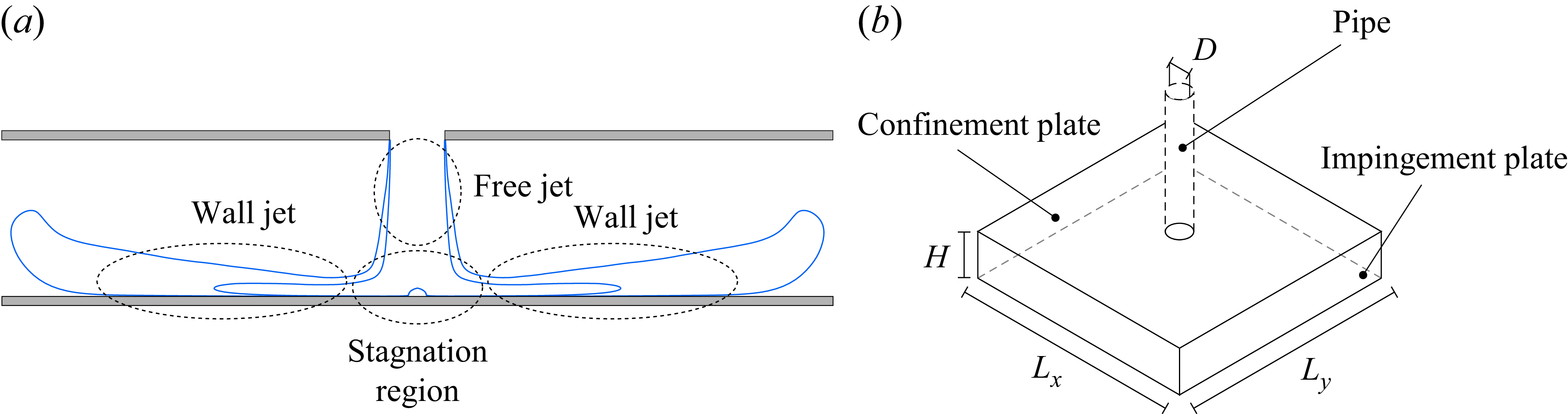

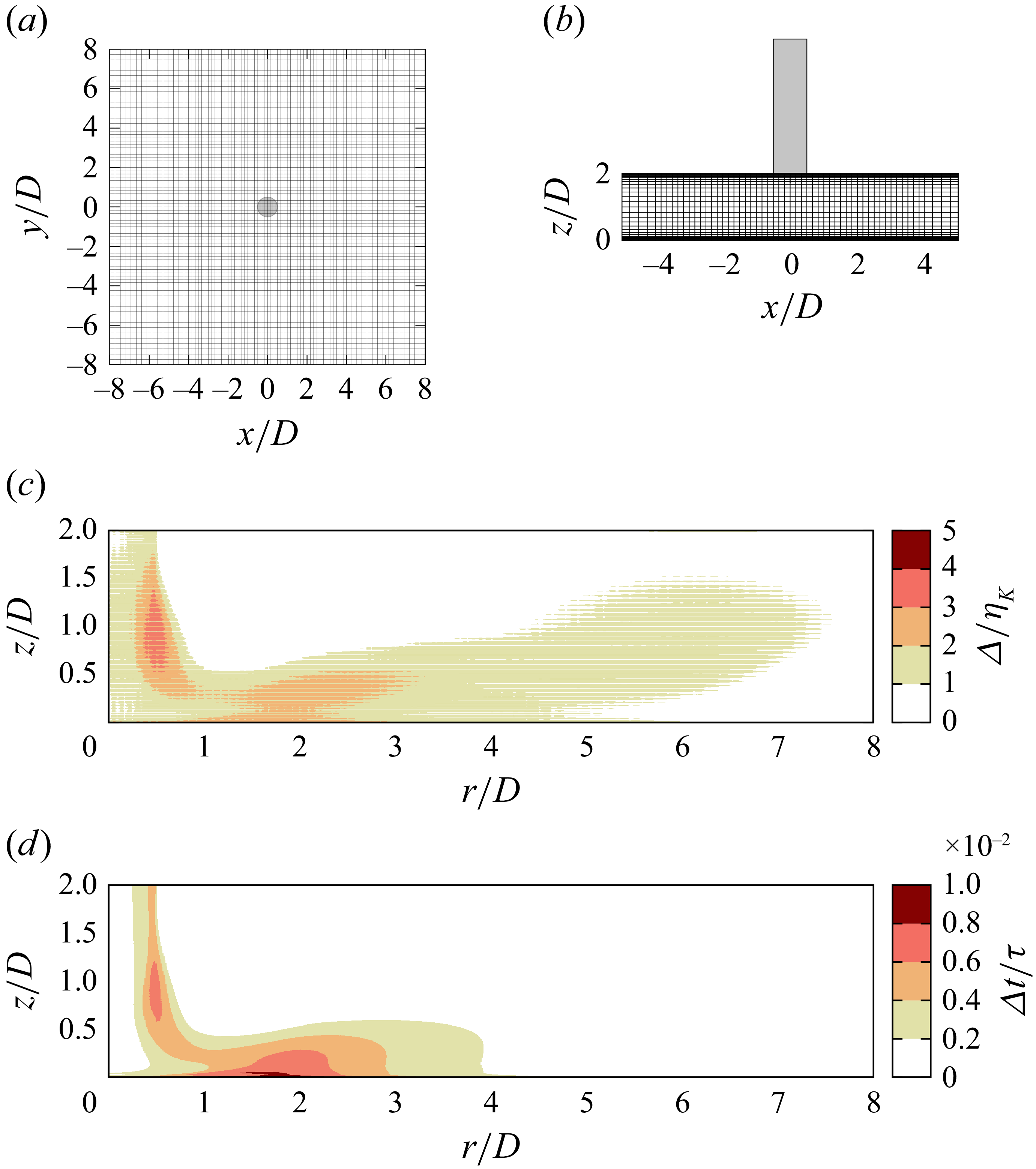
 x∈[−5,5]
 Δ/ηK
 Δt/τ
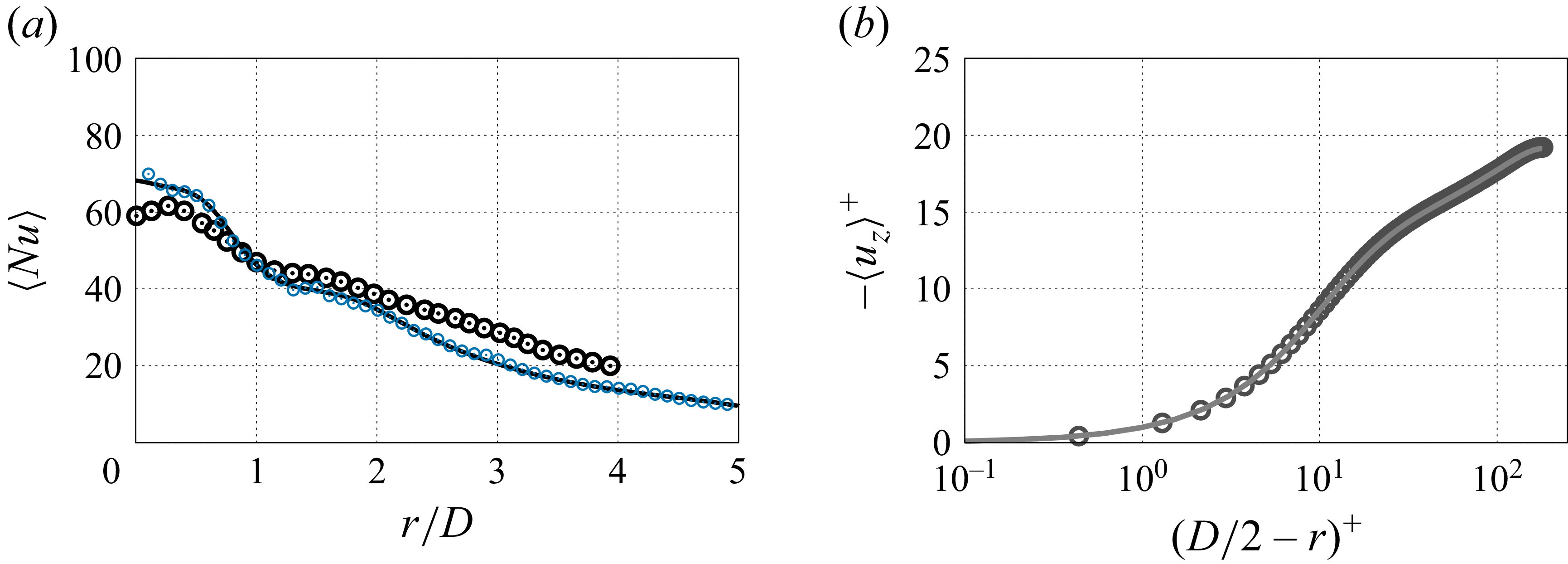
 N=7
 N=5

 z=0.1D
 ⟨ur′ur′⟩/Ub2
 ⟨uϕ′uϕ′⟩/Ub2
 ⟨uz′uz′⟩/Ub2
 ⟨ur′uz′⟩/Ub2
 Lx=Ly=16D
 Lx=Ly=20D

 ⟨ur⟩/Ub
 ⟨uz⟩/Ub
 ⟨ur⟩
 ⟨uz⟩

 ⟨ur⟩/Ub
 ⟨θ⟩
 zm/D
 zθm/D
 zΘm/D

 r/D=0.25
 r/D=1
 r/D=2
 r/D=3
 NLr/(Ub2/D)
 Gr/(Ub2/D)
 Vr/(Ub2/D)
 NLz/(Ub2/D)
 Gz/(Ub2/D)
 NLθ/(Ub/D)
 Vθ/(Ub/D)
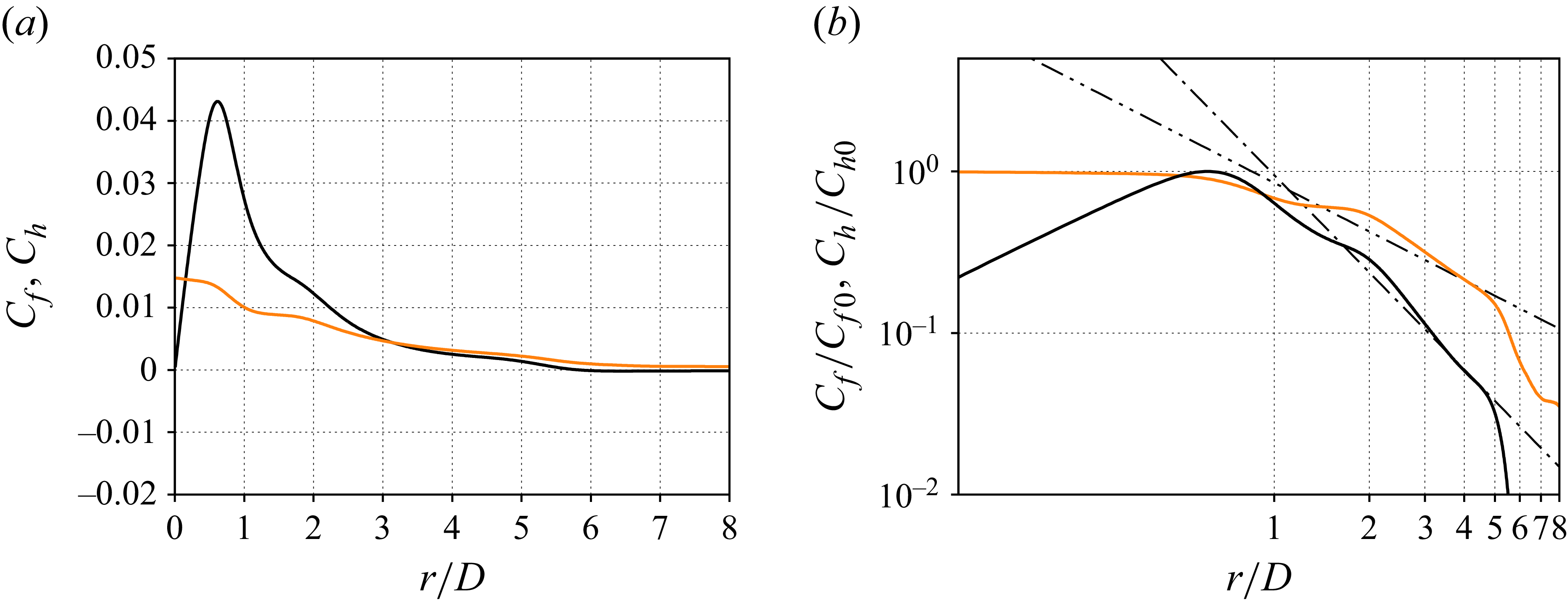
 Cf
 Ch
 Cf/Cf0
 Ch/Ch0
 ∼(r/D)−2
 ∼(r/D)−1
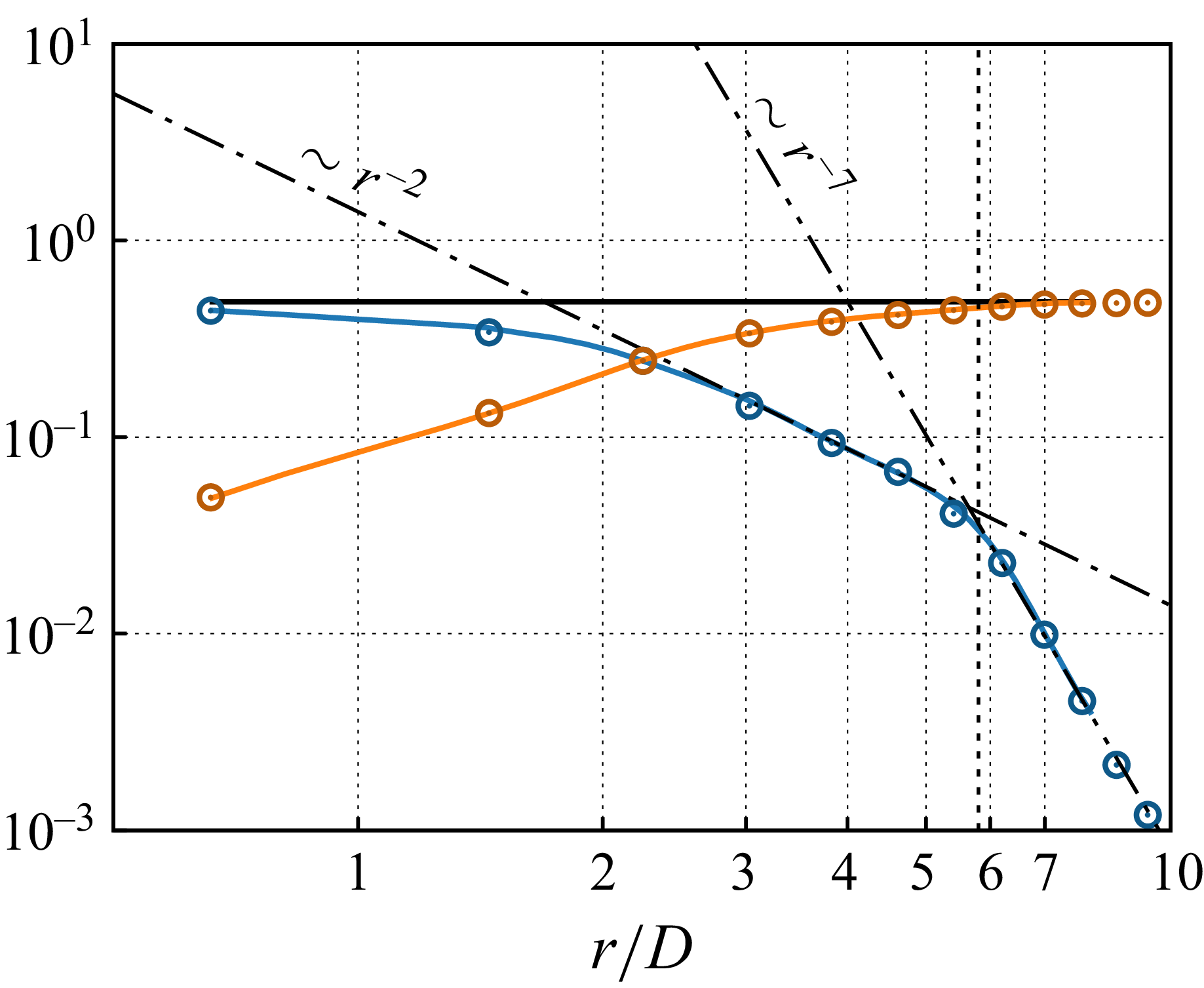
 Lx=Ly=16D
 Πin/(Ub3D2)
 Πout/(Ub3D2)
 E/(Ub3D2)
 Lx=Ly=20D
 Πout/(Ub3D2)
 E/(Ub3D2)
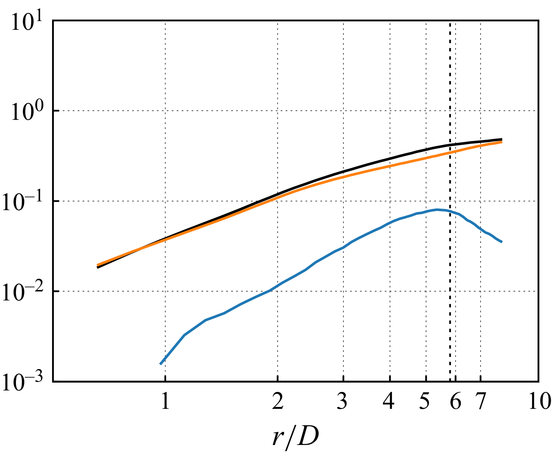
 Γ
 θwΠθ/(UbD2)
 ΠΓout/(UbD2)
 EΓ/(UbD2)

 ηUb2/(cpΔT)
 Ub2(Πθ(r)−ΠθB)/E(r)
 Ub2Πθ(r)/E(r)
 η~Ub2/(cpΔT)

 ν⟨ω⟩⋅⟨ω⟩D/Ub3
 α⟨∇θ⟩⋅⟨∇θ⟩D/Ub
 ν⟨ω′⋅ω′⟩D/Ub3
 α⟨∇θ′⋅∇θ′⟩D/Ub
 zm/D
 zθm/D

 ur′/Ub
 z=0.005D
 0.2
 1.0
 νω′⋅ω′D/Ub3
 α∇θ′⋅∇θ′D/Ub

 D[E]/([V]Ub3)
 D[Em]/([V]Ub3)
 D[Et]/([V]Ub3)
 D[EΓ]/([V]Ub)
 D[EΓm]/([V]Ub)
 D[EΓt]/([V]Ub)

 Open access

